Article

An Improved Principal Component Analysis Method for the Interpolation of Missing Data in GNSS-Derived PWV Time Series

1
College of Surveying and Geo-Informatics, North China University of Water Resources and Electric Power, Zhengzhou 450046, China
2
State Key Laboratory of Geo-Information Engineering, Xi’an 710054, China
3
School of Environment Science and Spatial Informatics, China University of Mining and Technology, Xuzhou 361000, China
4
College of Water Resources, North China University of Water Resources and Electric Power, Zhengzhou 450046, China
5
Satellite Positioning for Atmosphere, Climate and Environment (SPACE) Research Centre, RMIT University, Melbourne, VIC 3001, Australia
6
Chinese Academy of Engineering, Beijing 100088, China
7
Henan Provincial Key Laboratory of Hydrosphere and Watershed Water Security, North China University of Water Resources and Electric Power, Zhengzhou 450046, China
*
Author to whom correspondence should be addressed.
Remote Sens. 2023, 15(21), 5153; https://doi.org/10.3390/rs15215153
Submission received: 5 September 2023 / Revised: 25 October 2023 / Accepted: 25 October 2023 / Published: 28 October 2023
(This article belongs to the Section Atmospheric Remote Sensing)

Abstract

:
Missing data in precipitable water vapor derived from global navigation satellite systems (GNSS-PWV) is commonly a large hurdle in climatical applications, since continuous PWV is an important prerequisite. Interpolation using principal component analysis (PCA) is typically used to resolve this problem. However, the popular PCA-based interpolating methods, e.g., rank-deficient least squares PCA (RDPCA) and data interpolating empirical orthogonal function (DINEOF), often lead to unsatisfactory results. This study analyzes the relationship between missing data and PCA-based interpolation results and proposes an improved interpolation-based RDPCA (IRDPCA) that can take into account the PWV derived from ERA5 (ERA-PWV) as an additional aid. Three key steps are involved in the IRDPCA: initially interpolating missing data, estimating principal components through a functional model and optimizing the interpolation through an iterative process. Using a 6-year GNSS-PWV over 26 stations and ERA-PWV in Yunnan, China, the performance of the IRDPCA is compared with the RDPCA and DINEOF using simulation experiments based on both homogeneous data (i.e., interpolating ERA-PWV using available ERA-PWV) and heterogeneous data (i.e., interpolating GNSS-PWV using ERA-PWV). In the case of using homogeneous data, the root mean square (RMS) values of the interpolation errors are 3.45, 1.18 and 1.17 mm for the RDPCA, DINEOF and IRDPCA, respectively; while the values are 3.50, 2.50 and 1.55 mm in the heterogeneous case. These results demonstrate the superior performance of the IRDPCA in both the heterogeneous and homogeneous cases. Moreover, these methods are also applied to the interpolation of the real GNSS-PWV. The RMS, absolute bias and correlation of the GNSS-PWV are calculated by comparison with ERA-PWV. The results reveal that the interpolated GNSS-PWV using the IRDPCA is not impacted by the systematic discrepancies in the ERA-PWV and agrees well with the original data.

Graphical Abstract

1. Introduction

Water vapor, as a crucial greenhouse gas, significantly impacts the global energy balance and hydrological cycle through its evaporation, transport and condensation. Its positive feedback mechanism with temperature changes further exacerbates climate change and contributes to global warming [1,2,3,4]. Therefore, the monitoring of the content of water vapor, typically measured by precipitable water vapor (PWV), and assessment of its historical changes are crucial in the climatic field. Radiosonde data are the most commonly used for obtaining PWV due to the high accuracy and long historical records [5,6]. However, it has several limitations such as low temporal resolution, high cost and potential bias in extreme environments [7]. With the rapid development of satellite and observation technology, global navigation satellite systems (GNSS) and remote sensing images are increasingly popular. Remote sensing images can provide continuous PWV in the spatial domain [8,9,10,11]. However, they are easily influenced by various factors, e.g., clouds, smoke, atmospheric aerosols and the methodologies, thus resulting in low-accuracy PWV retrievals [11,12,13]. Compared to the remote sensing images, using high-accuracy GNSS observations to estimate PWV is more frequently used in PWV retrieval due to its low cost, high temporal continuity and global coverage [14,15,16,17]. Nowadays, GNSS-PWV has gained scientific significance and has been applied in the analysis of the variation in long-term PWV time series [18,19,20,21]. Extracting signals from evenly sampled GNSS-PWV time series without any missing data (i.e., data gaps) using either parametric or nonparametric methods is a prerequisite for this type of analysis [22]. However, missing data often occur because of various factors, e.g., upgrading of GNSS receivers, interruption of signals and intense geological activities. In these cases, the missing data need to be interpolated to reconstruct a complete and evenly sampled GNSS-PWV time series, which can be used for related application fields.
There have been several studies on interpolation for missing data in a GNSS-PWV series. Wang et al. [23] used an enhanced singular spectrum analysis for such an interpolation based on the temporal features of GNSS-PWV. Alshawaf et al. [24] employed a harmonic model and a first-order autoregressive process as the function and stochastic model, respectively, to interpolate a GNSS-PWV time series with data gaps. Yang et al. [25] used a GNSS-PWV time series from surrounding GNSS stations and the interpolation methods of inverse distance weighted (IDW), ordinary kriging and thin plate splines (TPS) based on the global pressure and temperature 2 wet (GPT2w) model. These studies primarily focused on a case in which the GNSS-PWV time series of interest has sufficient reference data from its surrounding GNSS stations for interpolation. However, in reality, the data from surrounding GNSS stations are not sufficient for interpolating missing data. To address this issue, some scholars have proposed using observations from other techniques such as the interferometric synthetic aperture radar (InSAR) technique for the interpolation of GNSS-PWV [26,27]. However, these approaches may not be able to obtain a desired interpolation result for some reasons, e.g., InSAR data cannot provide absolute PWV values.
The ERA5 reanalysis dataset, which is an output of a numerical weather model and incorporates various meteorological observations, can provide continuous PWV (ERA-PWV) in both spatial and temporal scales with satisfactory accuracy [28]. With its spatial continuity, principal component analysis (PCA), or named empirical orthogonal function (EOF) in some disciplines, is suitable for processing the interpolation of data gaps [29,30,31,32]. Several typical PCA-based approaches have been proposed for interpolating missing data, such as data interpolating empirical orthogonal function (DINEOF) [30] and rank-deficient least squares PCA (RDPCA) [33]. DINEOF initially interpolates data gaps using zero values, calculates eigenvectors and eigenvalues and finally updates the filled zeros [30]. It performs well in the interpolation of homogeneous data and has been widely used in the interpolation of oceanographic data and remote sensing images [30,32]. RDPCA is another classical method that is primarily proposed for extracting the common mode components in GNSS coordinate time series with data gaps [34]. This method establishes a functional equation between the principal components (PCs) and nonmissing data in the original data; therefore, it excels at signal extraction from the gappy data. Additionally, these two methods are self-consistent methods for a single source of data but may lead to unsatisfactory interpolation results for heterogeneous data (e.g., ERA-PWV and GNSS-PWV) due to their systematic error. In this study, the effect of the initially interpolated values on the final interpolated result at the data gaps is analyzed and a new PCA-based method for interpolating GNSS-PWV using the ERA5 reanalysis dataset is proposed. The key advantage of the new method is its effectiveness in preserving the unique characteristics of GNSS-PWV time series and its improved interpolation results for both homogeneous and heterogeneous data.
This paper is organized as follows. Section 2 introduces the typical PCA methods (including the standard PCA method, DINEOF and RDPCA), presents a theoretical analysis and proposes a new PCA-based method for interpolating missing data in GNSS-PWV time series. Section 3 introduces the PWV data used in this paper. Section 4 evaluates the performance of the new and selected methods using both simulated and real GNSS-PWV data in Yunnan Province, China. Finally, the conclusion is drawn in Section 5.

2. Methods

2.1. Standard PCA

PCA can be implemented using either direct singular value decomposition (SVD) of the original data or an eigenvalue decomposition (ED) of its covariance matrix. Both approaches produce identical results in a case in which there are no missing values in a dataset. In this study, considering that the latter is usually applied to geodetic applications related to GNSS data [35,36,37], the ED approach was adopted.
Suppose X is an m × n demeaned PWV data matrix, where m and n denote the observation epochs and numbers of stations ( m n ), respectively. When there are no missing data in X , its covariance matrix is [36,37]
B = 1 m 1 X T X
or
B i , j = 1 m 1 k = 1 m X ( t k , i ) X ( t k , j )
where B is an n × n matrix containing the covariance values of PWV over stations i and j .
Subsequently, the eigen decomposition of B is conducted
B = V T Λ V
where V = [ v 1 , v 2 , , v n ] is an n × n orthonormal function basis matrix, and v is an orthogonal coefficient vector such that v i T v j = 0 for j i ; Λ = d i a g ( [ λ 1 , λ 2 , , λ n ] ) is the n × n diagonal eigenvalue matrix containing n eigenvalues, and the eigenvalues are arranged in descending order, i.e., λ 1 > λ 2 > > λ n .
The following equations can easily be deduced
B v k = λ k v k
X T X v k = ( m 1 ) λ k v k
Then, X can be projected onto the orthonormal function basis to derive the PCs
A = X V
where A = [ a 1 , a 2 , , a n ] is the m × n PC matrix.
Equation (6) can also be transformed into equivalent forms
a k = X v k
a k ( t ) = j = 1 n X ( t , j ) v k ( j )
The PC a k represents the temporal variations at the k-th station, which are affected by the common mode signals. The eigenvector v k with eigenvalue λ k carries the spatial response to a k . Furthermore, those PCs with higher eigenvalues account for more variations of X , and therefore, the first few PCs corresponding to the highest few eigenvalues are applied to the construction of the data matrix
X r c = k = 1 p a k v k T
or, in an equivalent form
X r c = [ a 1 , a 2 , , a p ] [ v 1 , v 2 , , v p ] T
X r c ( t i , j ) = k = 1 p a k ( t i ) v k ( j )
where X r c is the reconstructed data matrix; p is the number of selected PCs. In practice, p < n is usually adopted, which is determined with sufficient data variations
R = k = 1 p λ k / k = 1 n λ k

2.2. Modified PCA for Gappy Data

PCA is a feasible approach that can simplify the questions to extract the major information only when the observations cover the same period and do not contain any missing data. Nevertheless, it may not be practical for real-world applications; thus, the calculation and the following decomposition of the covariance matrix B can not be performed. To address this issue, two alternative strategies have been applied: (1) altering missing values in the original gappy data matrix using interpolation techniques, which allows for the regular calculation and decomposition of the covariance matrix [30,31,32,38]; (2) calculating the covariance matrix using the available nonmissing data and conducting eigenvalue decomposition based on the functional relationship between the nonmissing and the eigenvectors [34]. The typical methods of these two strategies are the DINEOF [30,39] and RDPCA [34].

2.2.1. DINEOF

The DINEOF initially fills data gaps with an unbiased guess (e.g., zeros for most of the applications suggested by several scholars) and then iteratively reconstructs a data matrix using SVD. The initially filled data in the gap are replaced with the reconstructed values in the iteration process [30,31,38]. The procedure for the DINEOF is summarized below.
(1)
The missing values in the original data matrix are all initialized to zero. Then, a subset of the nonmissing data in the original data matrix is selected through a Monte Carlo simulation and retained in a separate matrix for the purpose of validation in a later stage (i.e., as the reference or truth of the interpolation results). The selected data in the original data matrix are treated as missing data and replaced with zeros.
(2)
SVD is used to decompose the above data matrix to obtain eigenvectors and eigenvalues. The eigenvector that possesses the largest eigenvalue is used to reconstruct a new data matrix, on which the above procedure is then applied for the next decomposition and reconstruction process. This iterative process continues until the difference of the root mean square (RMS) values at missing data points between two adjacent iterations falls below a predefined criterion (0.001 is set in this study). Then, the interpolated data are compared with the reference data at those selected reference data points and their differences are used to calculate the RMS.
(3)
After the above data matrix is constructed, the number of eigenvectors is changed, and the above process is repeated several times for new RMS values for different numbers of eigenvectors selected. Then, the optimal number of eigenvectors is determined by cross-validation using the minimum RMS of the interpolated value. The interpolated data matrix resulting from the optimal number of eigenvectors that has no gaps can be well determined.

2.2.2. RDPCA

Unlike DINEOF, which is an interpolation-based method, RDPCA does not alter the original data matrix [33,34]; instead, it computes the elements of the covariance matrix B using the available nonmissing data as follows
{ B i , i = 1 m i 1 k = 1 m i X ( t k , i ) X ( t k , i ) B i , j = 1 m i , j 1 k = 1 m i , j X ( t k , i ) X ( t k , j )
where m i denotes the number of available data at the i station during the period studied; m i , j denotes the number of available data simultaneously at the i and j stations during the period.
B can be decomposed for the eigenvalues and eigenvectors based on Equation (3), and the following equation can be constructed based on Equations (8) and (11)
L ( t k ) = A ( t k ) ξ ( t k )
where ξ ( t k ) is the unknown vector consisting of the values of all of the PCs at epoch t k , L and A are a known vector and a known coefficient matrix, respectively. Suppose S i denotes the ensemble of the stations that have available data at epoch t k , then ξ ( t k ) , L and A are expressed as
ξ ( t k ) = [ a 1 ( t k ) , a 2 ( t k ) , , a n ( t k ) ] T
L ( t k ) = [ j S i X ( t k , j ) v 1 ( j ) , j S i X ( t k , j ) v 2 ( j ) , , j S i X ( t k , j ) v n ( j ) ] T
A ( t k ) = [ 1 j S i v 1 2 ( j ) j S i v 1 ( j ) v 2 ( j ) j S i v 1 ( j ) v n ( j ) j S i v 2 ( j ) v 1 ( j ) 1 j S i v 2 2 ( j ) j S i v 2 ( j ) v 2 ( j ) j S i v n ( j ) v 2 ( j ) j S i v n ( j ) v 2 ( j ) 1 j S i v n 2 ( j ) ]
When no missing data exist at t k , A ( t k ) is an identity matrix; otherwise, A ( t k ) is a rank-deficiency matrix since its rank equates to the number of available data at t k . Therefore, the equation generalizes the two cases: with and without missing data in the original data matrix. In the cases with missing data, ξ ( t k ) can be estimated using the rank-deficient least squares method
ξ ( t k ) = Σ A T ( t k ) [ A T ( t k ) Σ A ( t k ) ] L ( t k )
where [ ] denotes the pseudo-inverse; Σ is the covariance matrix of L ( t k ) whose nonzero values are on its diagonal and Σ i j = λ i κ i j ; and κ is the Kronecker symbol.

2.3. Effect of Missing Data on PCA

While both RDPCA and DINEOF are used to carry out interpolation through different strategies, their performances are different, especially in different scenarios. RDPCA fills missing data using a functional relationship between available data and PCs, whereas the DINEOF iteratively fills zeros and performs SVD decomposition. As a result, the DINEOF excels at signal extraction while the RDPCA performs better on interpolation. However, both methods have been applied only to single-source data due to the consideration that a systematic bias may exist among multisource data. For convenience but without loss of generality, we refer to the error (i.e., the difference of the initially filled data from their real data) caused by systematic bias and/or other potential errors, if any, as “initial error”. This error affects the reconstructed data matrix and is referred to as “reconstruction error”. While Beckers [30] conducted an error analysis based on SVD using the ED method, there was no comprehensive analysis of the effect of the initial error on the reconstruction error. Therefore, in this study, we conducted a theoretical investigation of the mechanism on how the initial error can be incorporated into the reconstruction error from the perspective of ED method.
Let δ X be the initial error in the data matrix, and after an iteration, the reconstructed data matrix is perturbated as
X = X ˜ + δ X
The perturbated PC, eigenvector and eigenvalue are
a k = a ˜ k + δ a k
v k = v ˜ k + δ v k
λ k = λ ˜ k + δ λ k
where a ˜ k , v ˜ k and λ ˜ k are the true values of the k-th PC, eigenvector and eigenvalue, respectively.
Based on Equation (9), the reconstructed data matrix using p PCs is
X r c = k = 1 p a ˜ k v ˜ k T = k = 1 p ( a k v k T + a k δ v k T + δ a k v k T )
where X r c is the direct form of the reconstructed data matrix when δ X exists. The following section will simplify the equation and clearly show the impact of δ X .
Note that the perturbated parameters still satisfy Equations (4), (5) and (7). Substituting Equations (16), (18) and (19) into Equation (5), and applying Equations (5) and (7) provides
δ X T X ˜ v ˜ k + X ˜ T δ X v ˜ k + X ˜ X ˜ T δ v k = ( m 1 ) ( λ ˜ k δ v k + δ λ k v ˜ k )
Multiplying the above equation by v k T , the perturbation in the k-th eigenvalue is
δ λ k = 2 v ˜ k T δ X T X ˜ v ˜ k m 1
This equation indicates the relationship between the initial error and eigenvalue, which introduces a perturbation, δ λ k , into the real value. It is also worth noting that the covariance matrix B of the data matrix represents the variation of the original data matrix, and the sum of all eigenvalues is identically equal to the trace of B . As a result, δ λ k may affect other eigenvalues and, ultimately, results in an incorrect determination of the number of PCs in Equation (12). It can also explain why the RDPCA has a relatively poor performance in interpolation. When adapting the RDPCA, the covariance matrix B is calculated only based on the part of the nonmissing data, which results in a loss of data variations and lowers the trace of B in comparison to the true values. In contrast, the DINEOF (or other interpolation-based methods) uses zeros to interpolate the missing data, which makes the initial interpolation retain some variations and benefits the covariance matrix B and the final interpolation.
In addition, the perturbated eigenvectors remain orthogonal to each other and their inner products are units, i.e.,
( v ˜ k + δ v k ) T ( v ˜ k + δ v k ) = 1 ( v ˜ k + δ v k ) T ( v ˜ i + δ v i ) = 0
Neglecting higher-order terms and introducing v ˜ k T v ˜ k = 1 yields
δ v k T v ˜ k + v ˜ k T δ v k = 0
δ v k T v ˜ i + v ˜ k T δ v i = 0
Equation (24) implies that the perturbation, δ v k , is orthogonal to its true value, v ˜ k ; thus, δ v k can be uniquely written using the orthogonal basis of v ˜ k as
δ v k = j k n α j k v ˜ j
where α j k is a coefficient reflecting the contribution of the eigenvector v ˜ j to the perturbation in v ˜ k . This equation shows that the perturbated eigenvector δ v k is a linear combination of other eigenvectors, and its effect can be analyzed using the coefficient α j k . If α j k is insignificant, the effect of the perturbation is neglectable. Therefore, it can be deduced how much δ X affects α j k .
Multiplying Equation (21) by v ˜ j T and also considering Equations (4), (5) and (7) provides
v ˜ j T δ X T a ˜ k + a ˜ j T δ X v ˜ k = ( m 1 ) ( λ ˜ k λ ˜ j ) α j k
Similarly, swapping indices j and k leads to
v ˜ k T δ X T a ˜ j + a ˜ k T δ X v ˜ j = ( m 1 ) ( λ ˜ j λ ˜ k ) α k j
The left-hand sides of both Equations (27) and (28) are completely identical after a transposition; thus, the final estimator of α j k can be expressed as
α j k = α k j = v ˜ j T δ X T a ˜ k + a ˜ j T δ X v ˜ k ( m 1 ) ( λ ˜ k λ ˜ j )
The equation reflects that the value of α j k is highly related to the difference between λ ˜ k and λ ˜ j . If they are very close (i.e., λ ˜ k λ ˜ j 0 ), α j k is very large and, thus, considerably amplifies the effect of the perturbation in the data matrix δ X , even though their values may be insignificant. Also, δ X can be easily transformed to δ v k , which highly affects the stability of the eigenvector v ˜ k , and, therefore, causes a significant error in the reconstructed matrix  X r c .
Substituting Equations (16)−(18) into Equation (7), the k-th PC becomes
a ˜ k + δ a k = ( X ˜ + δ X ) ( v ˜ k + δ v k )
After Equation (7) is used and higher-order terms are neglected the perturbation in the k-th PC can be expressed as
δ a k = X ˜ δ v k + δ X v ˜ k
Thus, the third term on the right-hand side of Equation (20) is
δ a k v k T = ( X ˜ δ v k + δ X v ˜ k ) v k T = δ X v ˜ k v k T = δ X
Substituting Equations (26), (29) and (32) into Equation (20) yields the reconstructed data matrix
X r c = k = 1 p ( a ˜ k v ˜ k T + t k n α t k ( v ˜ k v ˜ j T + v ˜ j v ˜ k T ) + δ X ) = X ˜ r c + p δ X + k = 1 p ( j k n α j k ( v ˜ k v ˜ j T + v ˜ j v ˜ k T ) )
This equation is the final form of Equation (20), which shows the error in the final reconstruction data matrix. This error is composed of two parts: the second and third terms in Equation (33). The former amplifies δ X by p times and accounts for most of the reconstruction error. To reduce this part of the error, δ X  and p need to be restrained and optimized. Since the covariance matrix B is highly sensitive to outliers [38], bad initial values for missing data can lead to extreme values in δ X , distort the PCs and yield a poor result. Thus, in this study, the means of the ERA-PWV values from the surroundings of the GNSS station of interest, rather than zeros, were used for the initial values of the missing data points. This is related to the coefficient α t k , which is further inversely proportional to the difference between two eigenvalues. Thus, the absolute difference | λ ˜ k λ ˜ t | needs to be significant so that the impact of the latter part of the reconstruction error on the reconstructed data matrix can be reduced. Considering that the first few PCs correspond to the first largest eigenvalues, which possess most of the variations and can yield significant absolute values, the criterion in Equation (12) is set to 99.9% for the determination of an optimal p .
In addition, from an analysis of the relationship between the above two parts of errors and the initial error, we found that the former is deterministic, but the latter is relatively stochastic; thus, it makes the interpolation complex. In cases in which the lowest few eigenvalues are selected, | λ ˜ k λ ˜ t | may become insignificant and, ultimately, adversely affect the interpolation performance. This is the reason why Monte Carlo simulation is essential in the determination of an optimal number of PCs in the DINEOF.

2.4. IRDPCA

According to the above analysis and the ideas of the RDPCA and DINEOF, a new iterative PCA-based method is proposed in this study. Assuming that the number of GNSS stations and ERA5 grid points together is n, and the gappy observation vector of the GNSS-PWV time series covers m epochs, then the procedure for the new PCA-based method is as follows (also see the flowchart in Figure 1).
(a)
Center the gappy data vector of each station by removing the mean value of the available observations from all of the GNSS stations and ERA5 grid points. The centered observation vectors for all of the n stations and grid points are used to construct the m × n original data matrix X . Set the index of the station j to 1, i.e., assign j = 1 ;
(b)
Retain the above missing data at the j-th station in X ; use the mean of the PWVs derived from the surrounding reanalysis datasets to interpolate the missing data for the stations from the j + 1-th to n-th stations for their initial data matrix X j ;
(c)
Use Equation (13) to compute the covariance matrix B , and use Equation (14) to compute eigenvectors v 1 , v 2 , , v n , eigenvalues  λ 1 , λ 2 , , λ n and PCs a 1 , a 2 , , a n ;
(d)
Determine an optimal number of PCs based on Equation (12) and the criterion of 99.9%;
(e)
Reconstruct data matrix X r c j ;
(f)
If j n , go to step (b); otherwise, end the process and use those nonmissing data in the original data matrix to calculate the reconstruction error e r c j .
Since the new method initially fills missing values like the DINEOF and updates the reconstructed matrix using the RDPCA, it is named interpolation-based RDPCA (IRDPCA).

3. Data

Yunnan Province in China was chosen as the experimental area, and the ERA5 reanalysis dataset and GNSS observations at 26 GNSS stations in the province were used as our data source. More details on these data are presented in the following subsections.

3.1. ERA5 Reanalysis Data

The ERA5 is the latest reanalysis dataset released by the European Centre for Medium-Range Weather Forecasts (ECMWF). It provides hourly atmospheric variables on 37 vertical pressure levels with a spatial resolution of approximately 31 km [28]. The ERA-PWV and GNSS-PWV are two independent datasets, since the former is generated by assimilating observations using various techniques, except for ground-based GNSS.
ERA5-PWV can be obtained using
PWV ERA = 1 ρ w q g d P
where ρ w , g and P are the density of liquid water, gravity acceleration and atmospheric pressure, respectively; q is the specific humidity, which can be calculated by
q = 0.622 e P 0.378 e , e = R H 100 , e s = 6.112 exp [ 17.67 ( T 273.15 ) T 29.65 ]
where e and e s are the water vapor pressure and saturation water vapor pressure, respectively; R H and T are the relative humidity and atmospheric temperature, respectively.

3.2. GNSS Data

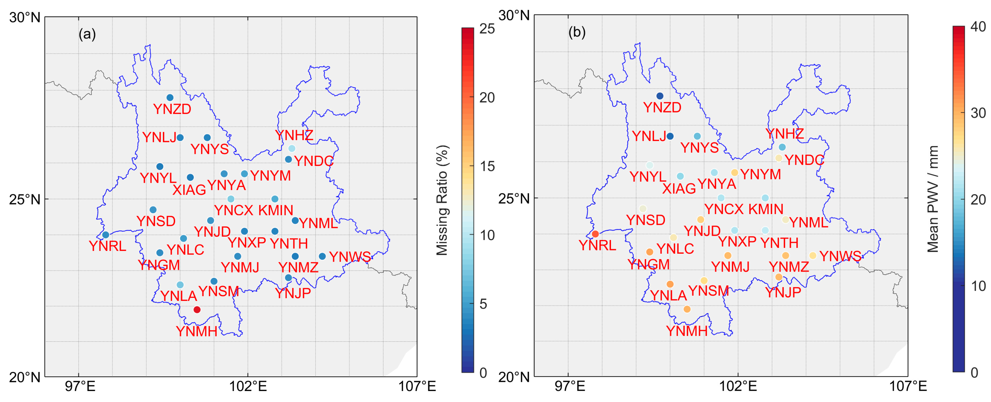
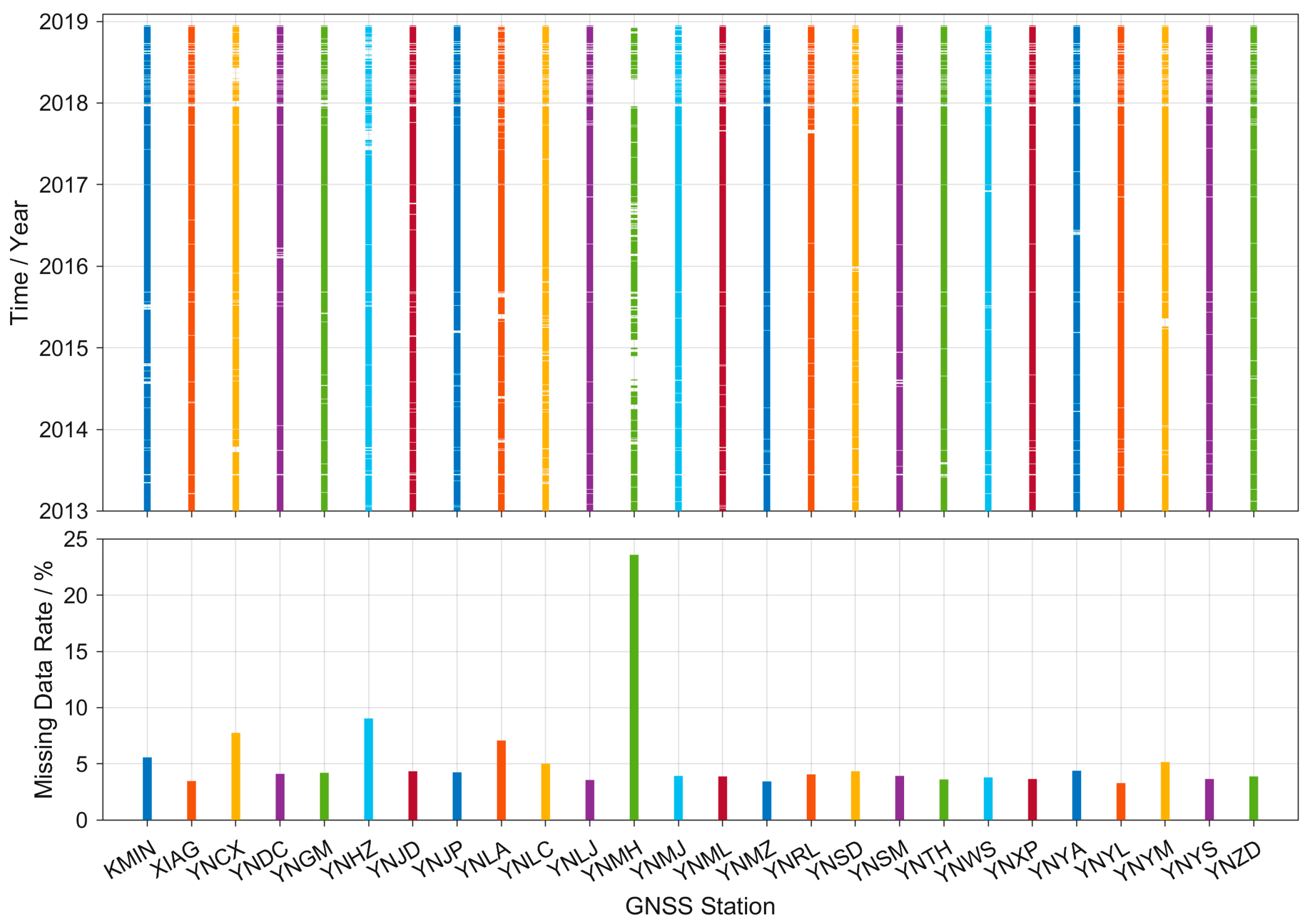
The GNSS-PWV time series used in this study was derived from hourly zenith tropospheric delay products at 26 GNSS stations selected from the Crustal Movement Observations Network of China in Yunnan Province. The ZTD products, spanning from 2013 to 2018 and processed using the GAMIT/GLOBK 10.4 software package, were provided with authority by the China Earthquake Administration. All of the ZTD time series were preprocessed to detect outliers using a range check between 1 and 3 m and an interquartile range. After the preprocessing procedure was carried out, the minimum, maximum and mean lengths of the remaining ZTD time series were 1674, 2119 and 2096 days, respectively, which were equivalent to missing data rates of 24.6%, 3.3% and 5.3%. The spatial distribution, annual mean PWV and missing data rates are shown in Figure 2 and Figure 3.
The remaining ZTD is converted to PWV using the following equation
PWV G N S S = 10 6 ( Z T D Z H D ) ρ R v ( k 2 + k 3 / T m )
where R v = 461.51   J / ( K kg ) ; k 2 = 16.52 K 2 / hPa ; k 3 = 3.776 × 10 5 K 2 / hPa ; ZHD is the zenith hydrostatic delay determined using the Saastamoinen model [40]; and T m is the weighted mean temperature. They are computed using
ZHD = 0.002769 P s 1 0.00266 cos ( 2 φ ) 0.00028 H
T m = e / T d h e / T 2 d h i = 1 N 1 e i / T i Δ h i i = 1 N 1 e i / T i 2 Δ h i
In the above conversion, atmospheric variable values obtained from the ERA5 dataset were used, since very few meteorological stations are available in Yunnan Province. To eliminate a potential nonclimatic bias in the selected GNSS-PWV time series, the homogeneity of the data series is tested and corrected with the absolute adaptive homogeneity test [41,42].

4. Results

To comprehensively analyze the performance of our proposed method, both simulated and real datasets were used in our experiments. The simulated data were used to assess the performance of both the heterogeneous and homogeneous data series. Specifically, the two types of simulations were (1) interpolation on the ERA-PWV time series only and (2) interpolation on the GNSS-PWV time series using the ERA-PWV time series. In addition, the real dataset, which was from the measurements, aimed to interpolate the missing data in the GNSS-PWV series with the aid of the ERA-PWV series.

4.1. Simulation Experiment

4.1.1. Simulation Using ERA-PWV

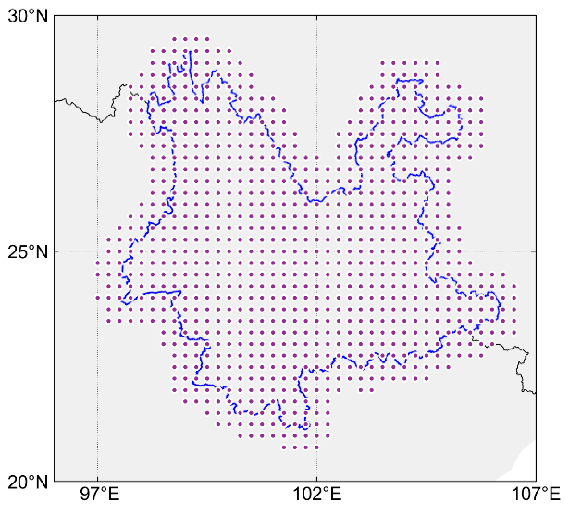
The first simulation experiment were performance comparisons of the previously mentioned three PCA-based methods on a homogeneous dataset using ERA-PWV values in Yunnan Province and its surrounding area. Figure 4 illustrates the spatial distribution of all of the grid points used in the interpolation. To simulate data gaps, various missing rates ranging from 0.1 to 0.6 with an interval of 0.1 were used. The missing data were “simulated” based on the original ERA-PWV time series (without missing data) by randomly selecting and removing some data points from the original data series. After the gappy ERA-PWV time series was simulated, the RDPCA, DINEOF and IRDPCA were applied to the interpolation for the missing data. Since PWV is highly correlated with geological elevation due to the vertical stratification of the neutral atmosphere [43], a 1° × 1° spatial window was used to release the geological influence on the PWV interpolation, and the missing data for all of the grids in this window were simultaneously interpolated. To compare the performances of the different methods, the simulation was run 30 times for each missing rate with the results of the calculated RMSs for the interpolation error (the difference between the interpolated and original data at the missing data points) and the reconstruction error (the difference between the interpolated and original data at nonmissing data points), see Figure 5.
Figure 5 shows the RMS of the interpolation and construction errors resulting from the three methods and various missing rates selected for the tests. The mean RMSs of the interpolation errors resulting from all of the selected missing rates and the RDPCA, DINEOF and IRDPCA methods were 3.45, 1.18 and 1.17 mm, respectively, while that of the reconstruction errors were 0.67, 1.15 and 1.06 mm. These results demonstrate that the RDPCA performed poorly on the interpolation but well in the reconstruction of the data matrices. This is consistent with our theoretical analysis that using nonmissing data for the RDPCA can result in a better reconstruction result but at the cost of losing the sum of real eigenvalues and unsatisfactory interpolation results. The DINEOF initially fills missing data using zeros, which benefits the eigenvalues and interpolation results. The IRDPCA utilizes an interpolation strategy similar to the DINEOF on the basis of the RDPCA, thus leading to a performance comparable to that of the DINEOF. In addition, the RMSs of the interpolation errors at the missing data points and the reconstruction errors at the nonmissing data points resulting from all three methods varied with the missing rate. However, the RMSs of the IRDPCA and the DINEOF exhibited similar variation trends and had a much smaller variation than the RDPCA. The much larger variation of the error values from the RDPCA implies a much higher sensitivity of this method to the missing rate than the other two methods. Therefore, we can conclude that the number of missing data points in a gappy series has a greater impact on the RDPCA, compared to the IRDPCA and DINEOF. In addition, the higher sensitivity of the RDPCA may also be attributed to the utilization of the nonmissing data only.
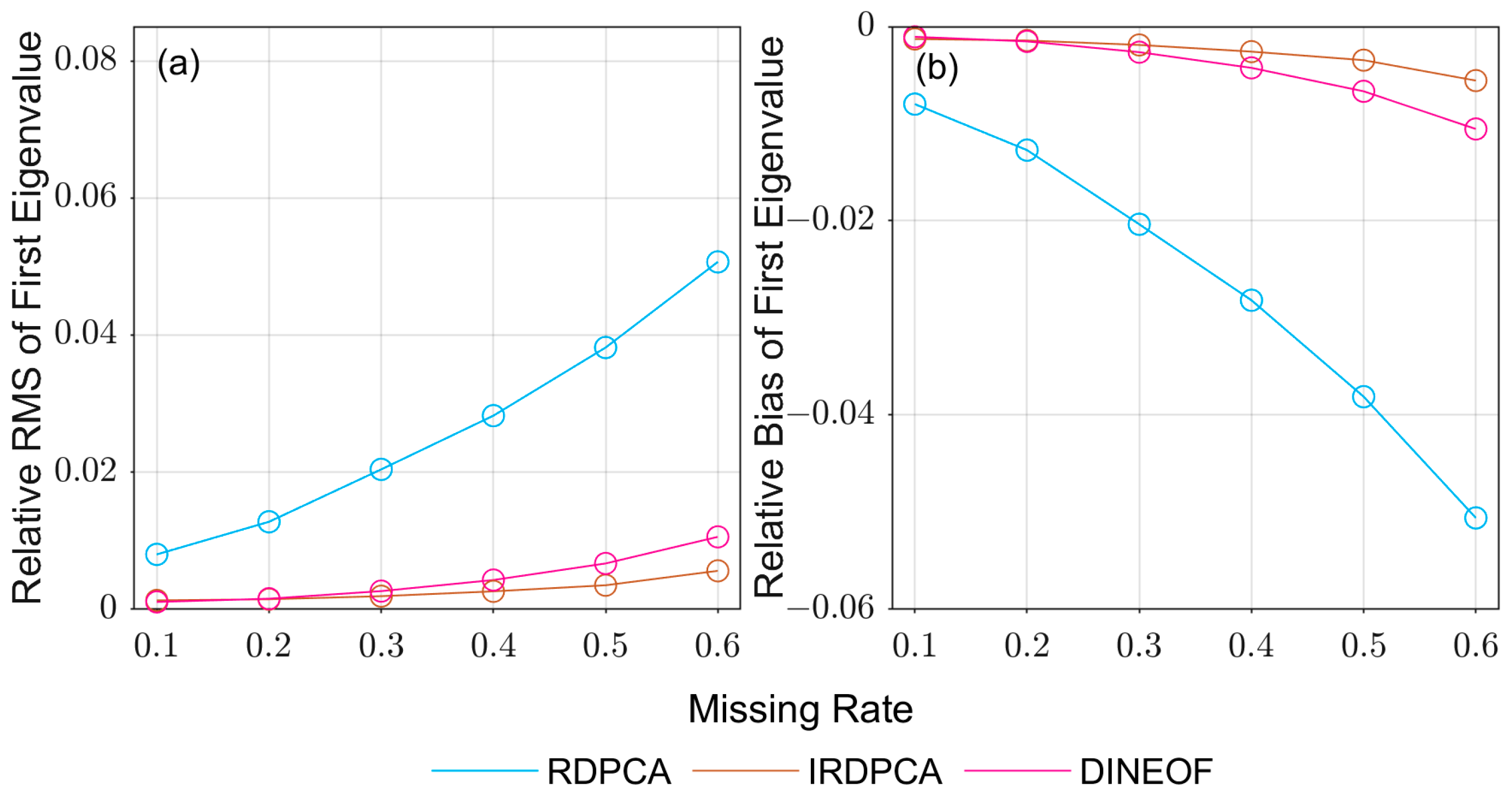
The first few eigenvalues possess most of the variations, so the first and second largest eigenvalues of the interpolated data were selected to analyze the performance of these methods. Figure 6 and Figure 7 illustrate the RMS and bias of the first and second largest eigenvalues, respectively. It should be noted that the RMS and bias values in both figures were relative values rather than the original ones, i.e., the ratio of the RMS and bias to their true eigenvalues. As shown in Figure 6, the relative RMSs and biases of the first eigenvalues show a positive relationship with the missing data rate, the poorest performance occurred in the largest missing rate (0.6%). For the RDPCA, the maximum values of the relative RMS and bias were 5% and −5%, while the values of the DINEOF and IRDPCA were 0.6%/−0.6% and 1%/−1%. It is obvious that the errors resulting from the DINEOF and IRDPCA were less influenced by the missing data rates. This phenomenon is consistent with the variation in the RMS of the interpolation errors, as the first largest eigenvalue contains the dominant variation in the PWV time series.
In Figure 7, the RDPCA results (in blue) show little direct correlation between the relative RMS/bias and the missing data rate, and one anomaly in the relative RMS occurs at a missing rate of 0.3 and one in the relative bias at a missing rate of approximately 0.4. However, the relative RMS and bias resulting from the other two methods (DINEOF in purple and IRDPCA in brown, respectively) are both strongly correlated with missing data rates. Furthermore, both figures show that the smallest relative RMS and bias resulted from our proposed IRDPCA method (brown), especially at the largest missing rate (60%), and the relative RMS of the first and second largest eigenvalues are only 0.6% and 1.8%, respectively. These results suggest that our method can effectively interpolate missing data and recover eigenvalues with high accuracy in the case of homogeneous data.

4.1.2. Simulation Using ERA5 and GNSS-PWV

The second simulation experiment was conducted on heterogeneous data, and data gaps were also simulated by randomly selecting and removing some data points from real GNSS-PWV time series (refer to Section 3.2), and the ERA-PWV data over four grid points surrounding the target GNSS station were utilized to complete the interpolation for the missing data in the GNSS-PWV. Since the inherent missing rates of the GNSS-PWV time series usually range from 3.3% to 9.0%; thus, a range from 5% to 40% (with a step of 5%) was set for the simulated missing rates. In addition, Yang et al. [25] pointed out that IDW, TPS and kriging based on GPT2w have satisfactory and comparable interpolation results. Therefore, IDW based on GPT2w (simplified as IDW) was employed in the simulation, and the result was compared with that of the aforementioned three PCA-based methods.
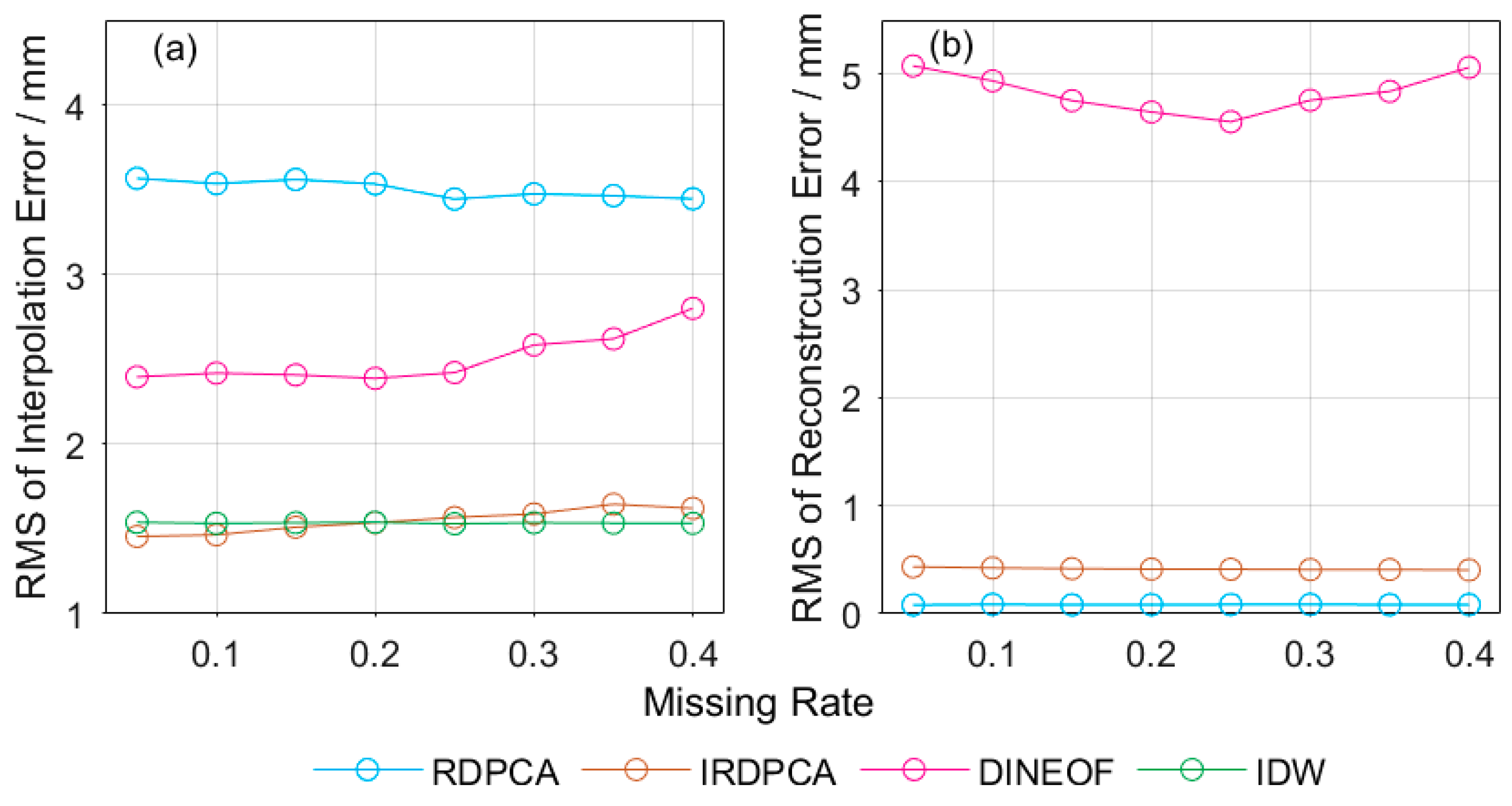
Figure 8 depicts the RMS of the interpolation error for the selected four methods, as well as the reconstruction error for the three PCA-based methods since the IDW method only involves interpolation. The means of the RMS values of the interpolation errors of all of the missing rates resulting from the RDPCA, DINEOF, IDW and IRDPCA were 3.50, 2.50, 1.54 and 1.55 mm, as shown in Figure 8a, respectively. It is evident that the DINEOF has a value much higher than that of the first simulation experiment, while the RDPCA and IRDPCA results were nearly comparable to the first experiment. The significant difference of the DINEOF in the two experiments suggests that the DINEOF may not produce satisfactory results for the heterogeneous data, such as using the ERA-PWV to interpolate missing data for the GNSS-PWV. In contrast, the results for both the IRDPCA (brown) and IDW (green) varied little with the missing rate, and the mean RMS values were 1.55 and 1.54 mm for the IRDPCA and IDW, respectively. The RMS values of their interpolation errors remained at approximately 1.5 mm. Their differences were that the IDW outperformed the IRDPCA a little for the simulations when the missing rates were more than 0.2, while the IRDPCA was the better method when the missing rates were less than 0.2. Figure 8b displays the variations in the RMS of the reconstruction error from three PCA-based methods with missing rates, and the means of the RMS values at all missing rates were 0.09, 4.83 and 0.42 mm for the RDPCA, DINEOF and IRDPCA, respectively. These results also demonstrate the satisfactory performance of the IRDPCA.
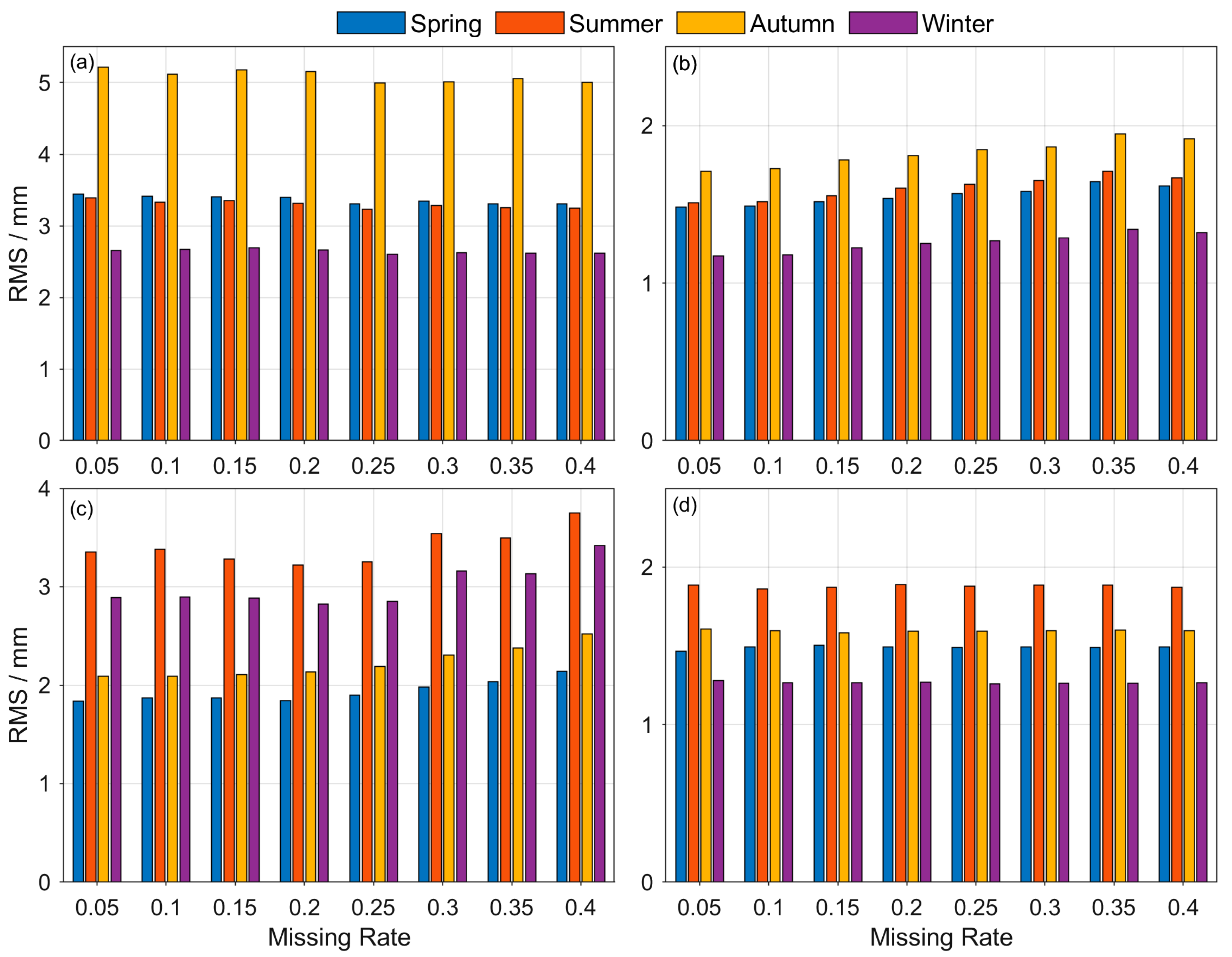
To investigate the impact of the temporal variation in the PWV time series on the interpolation results, the seasonal RMSs of the interpolation errors resulting from each missing rate and each method are compared in Figure 9. From Figure 9a,b, which are for the RDPCA and IRDPCA, respectively, we can see that the maximum and minimum RMS values occur in autumn (mean values are 5.1 and 1.8 mm for the RDPCA and IRDPCA) and winter (mean values are 2.6 and 1.3 mm for the RDPCA and IRDPCA), respectively; those from the DINEOF (Figure 9c) occur in summer and spring (mean values are 3.4 and 1.9 mm), respectively; while those from the IDW (Figure 9d) occur in summer and winter (mean values are 1.9 and 1.3 mm), respectively. Yunnan Province, located in a low-latitude inland area with a subtropical plateau monsoon climate, exhibits similar seasonal patterns where the maximum and minimum values occur in summer and winter, respectively. Therefore, the temporal distribution of the RMS from IDW appears to be well aligned with the temporal characteristics of the PWV, whereas the ones obtained from the three PCA-based methods do not agree well with these features. The reason for this discrepancy needs to be further investigated.
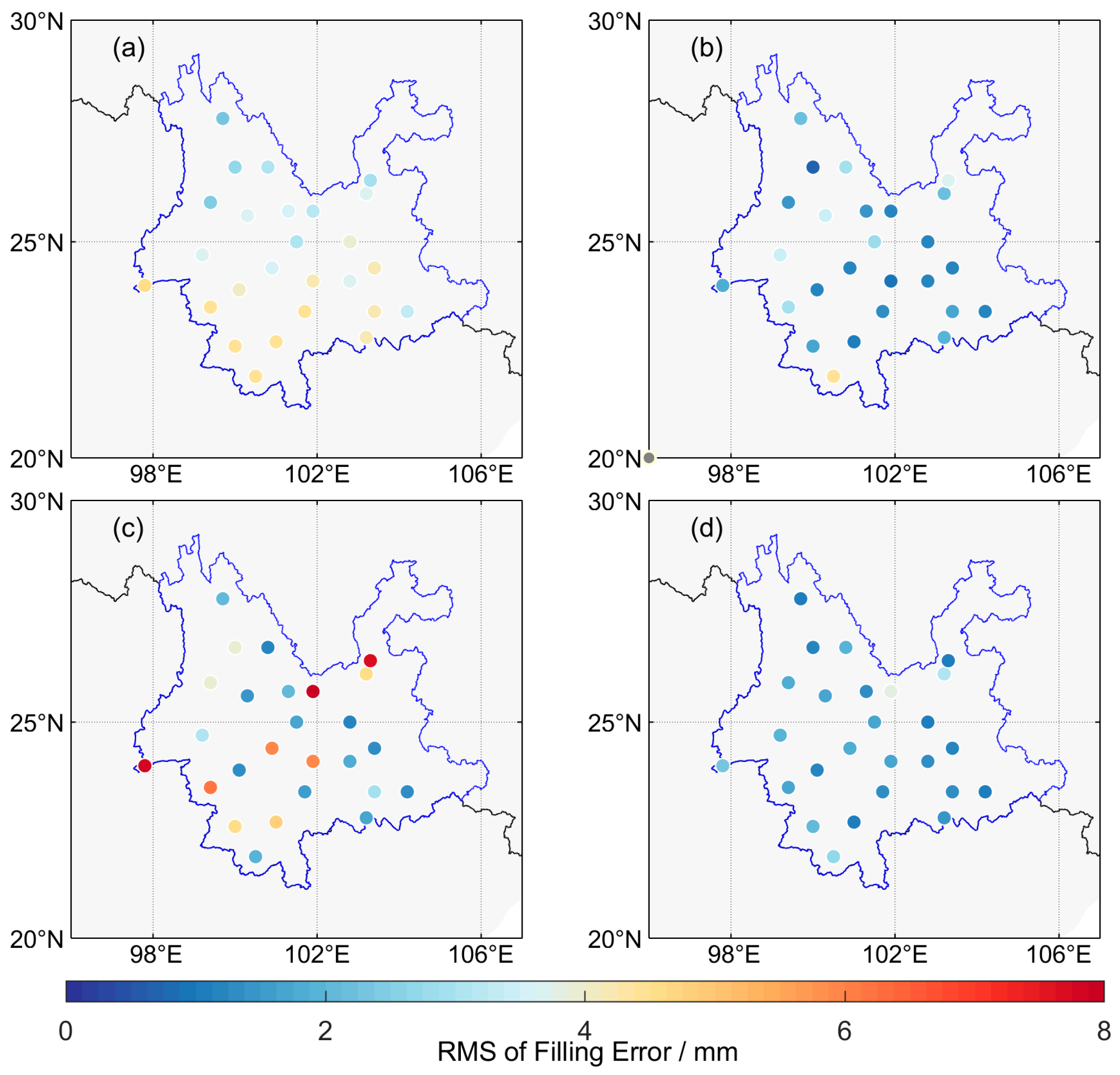
Figure 10 presents the RMS of the interpolation errors at each GNSS station from each of the four methods for an analysis of the spatial factors that influence the interpolation performance. Figure 10a shows a clear spatial distribution of the RMS from the RDPCA with larger RMS values (more than 4 mm) in the southern area, and the RMS value shows a decreasing trend from south to north, which is consistent with the spatial distribution of the annual mean PWV in Yunnan Province (shown in Figure 2b). Thus, the performance of the RDPCA is primarily influenced by the annual mean of the PWV. Figure 10b shows the RMS of the IRDPCA agrees well with the spatial distribution of the missing rates shown in Figure 2a. Specifically, the highest RMS was 4.5 mm, located at the YNMH station with a maximum missing rate of 24.6%, and the smallest RMS was 0.73 mm, located at YNLJ with a missing rate of 3.6%, which is almost the minimum missing rate value. Thus, it can be inferred that the missing rate is the main spatial factor affecting the performance of the IRDPCA. Figure 10c shows that the RMSs from the DINEOF at six stations were all above 5 mm; hence, the DINEOF is the worst performer. The RMSs from the IDW in Figure 10d were mostly under 2 mm and without significant spatial characteristics. In summary, the performances of the RDPCA and IRDPCA have some dependency on the annual mean of the PWV and also the missing rate of the original GNSS-PWV, while the influencing factors of the other two methods seem less clear.
The results of the above two simulation experiments reveal that our proposed IRDPCA method exhibits great performance on interpolation for missing data in both heterogeneous and homogeneous data, while the DINEOF is highly susceptible to systematic bias and performs well only on homogeneous data, and the RDPCA performs poorly.

4.2. Interpolation of Real GNSS-PWV Time Series

The above four methods were also applied to the interpolation for missing data in real (i.e., observed) GNSS-PWV time series at the aforementioned 26 GNSS stations in Yunnan Province. Considering a case in which there were no available observed (or truth) data (like the above simulation experiments) for the performance evaluation of these interpolation methods, a different strategy is needed. In this study, for the reference PWVs at the missing data points, we used the IDW interpolation method and the ERA-PWV values at the four grid points surrounding the target GNSS station to obtain the interpolated PWV for the GNSS station. Then, the above interpolated PWV from different methods and the nonmissing PWV at each of the 26 GNSS stations were compared to the ERA-PWV to calculate the RMS, absolute bias and correlation coefficient for the performance evaluation. In addition, the PWV derived from the radiosonde observations (RS-PWV) over the radiosonde station 56778, which is co-located with KMIN, was also used to calculate the statistical indexes.
Figure 11 shows the statistical results of the interpolated PWV using the four methods for each station. It should be noted that apart from the four results, an additional result (i.e., the difference between the original GNSS-PWV at those nonmissing data points and their corresponding reference ERA-PWV) is also shown in this figure. This can help us analyze the agreement between the original data and the interpolated data from these four methods. It can be observed that the RMS and absolute bias of the GNSS-PWV interpolated from the IDW were the smallest, and the correlation coefficients from this method were the highest among all of the four methods. However, compared to the statistical results of the original GNSS-PWV at the nonmissing data points, the RMS and absolute bias decreased by 77.5% and 79.7%, respectively, while the correlation coefficients increased by 7.5% and their values were close to 1. The results can be attributed to the same use of the IDW method when the reference ERA-PWV was calculated for the GNSS stations, reducing the systematic bias between the GNSS-PWV and reference ERA-PWV after the interpolation but leading to the inconsistent characteristic with the GNSS-PWV at the nonmissing data points. The DINEOF amplified the systematic bias, especially at YNHZ, YNRL, YNYL and YNYM, where the RMS and absolute bias of the interpolated GNSS-PWV were above 10 mm and 7 mm, respectively. The RDPCA also led to a significant discrepancy after the interpolation, with an approximately double increase in both the RMS and absolute bias. In contrast to these three interpolation methods, which led to large deviations from the original GNSS-PWV, most of the data interpolated from IRDPCA agreed well with the original GNSS-PWV, with a reduction of approximately 35.4% and 39.8% in the RMS and absolute bias, respectively, after the interpolation. These results suggest that our IRDPCA method well retained the characteristics of the GNSS-PWV at the nonmissing data points.
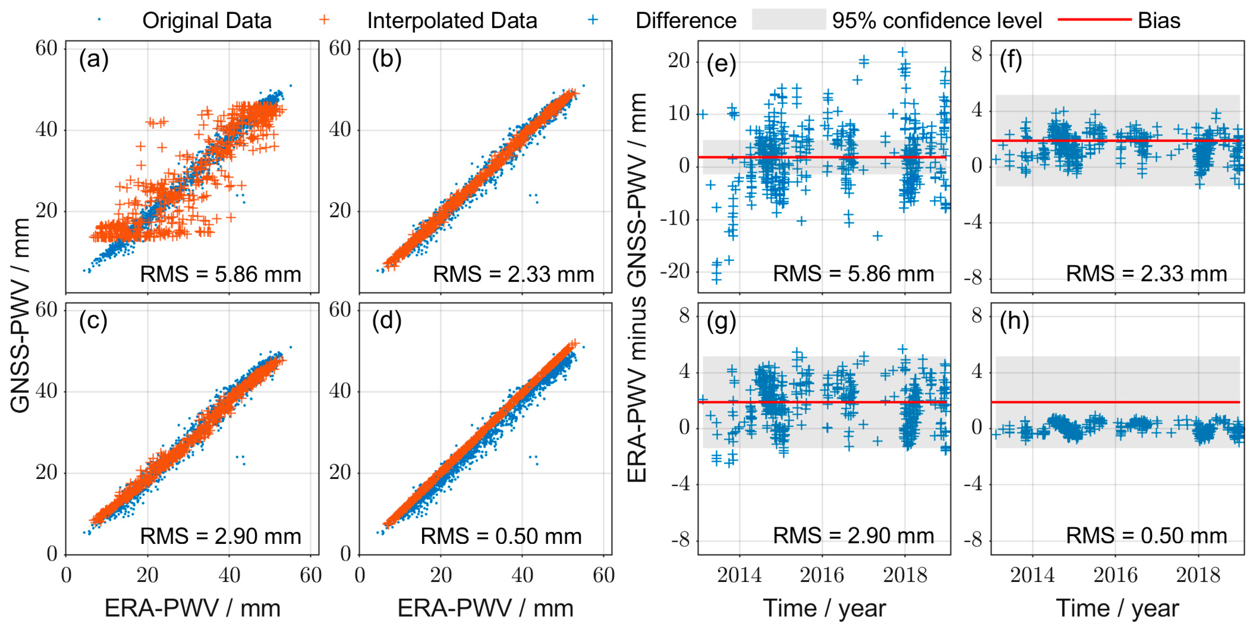
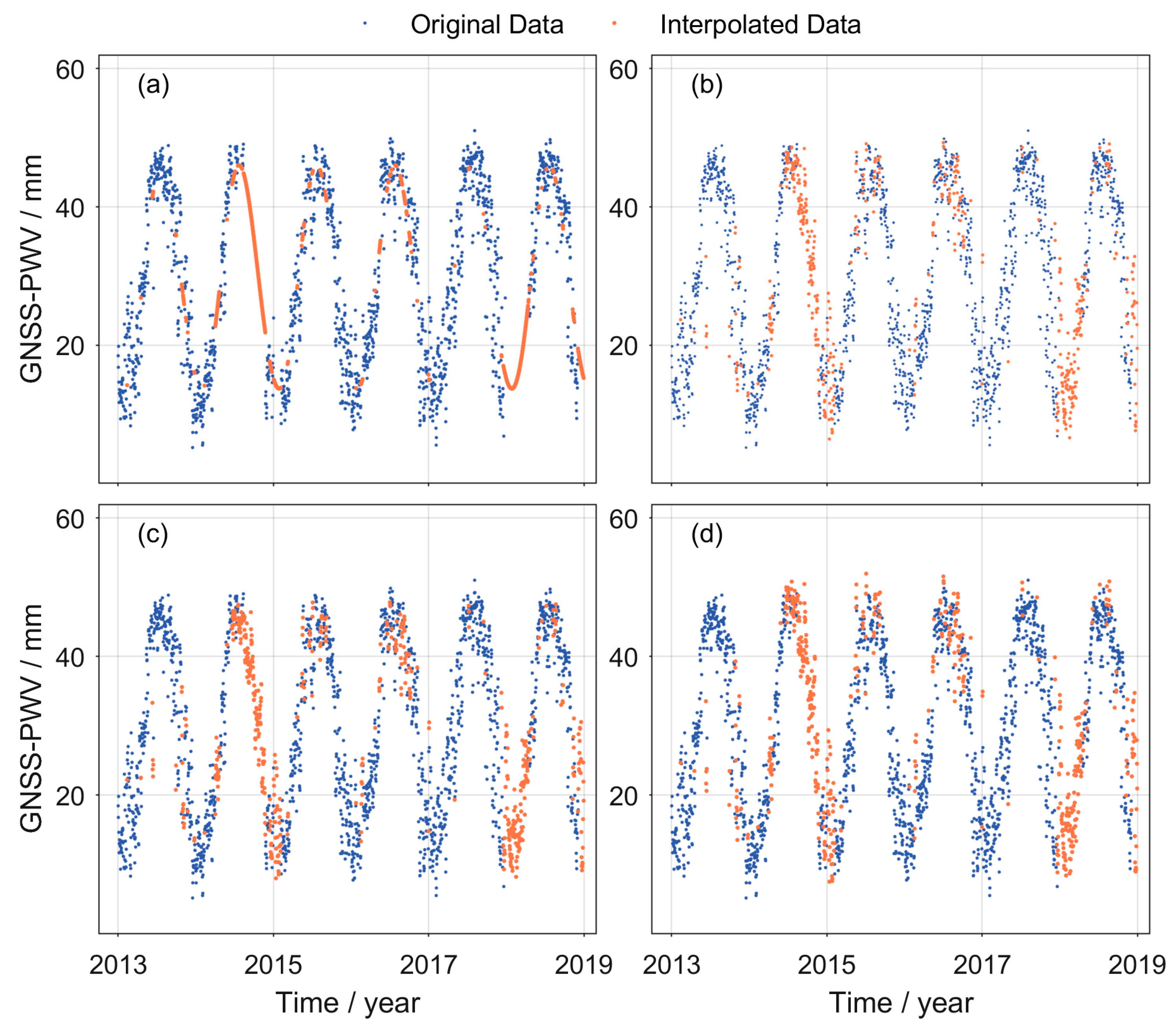
Figure 12 and Figure 13 show the scatter plots of the original and interpolated GNSS-PWV from the selected four methods versus the reference ERA-PWV over the YNMH station during the 6-year period from 2013 to 2018, which has continuous data gaps and considerably higher missing rate than other stations. As shown in Figure 12a and Figure 13a, the interpolation results from the RDPCA are smooth but significantly deviate from the range of values of the original GNSS-PWV at the nonmissing data points. This deviation may be caused by (1) the low correlation between the GNSS-PWV and ERA-PWV in a 1° × 1° spatial window, and (2) the potential unsuitability of the time series with a high missing rate. The RDPCA completes the interpolation based on the available nonmissing data, which can lead to a loss of the sum of the eigenvalues. The loss would influence the identification of the main principal components. For the PWV over YNMH, only several PCs with high eigenvalues (e.g., annual, semi-annual and seasonal signals) can be well identified using the RDPCA, and the high-frequency signals with low eigenvalues that are related to weather variations can be easily ignored. Therefore, the interpolation PWV is quite smooth.
The RMS values of the PWV interpolated from the IRDPCA and DINEOF were 2.33 and 2.90 mm, respectively, which are very close to that of the original GNSS-PWV (2.79 mm). However, comparing these two types of results, we can see a few systematic discrepancies between the original data and interpolated data obtained from the DINEOF, whereas the PWV interpolated from the IRDPCA in Figure 12 and Figure 13 agree well with the original PWV at nonmissing data points. It leads to the higher RMS values of the DINEOF compared with the IRDPCA. In addition, although the IDW led to the smallest RMS (0.50 mm) among the methods, the noticeable systematic discrepancies between the original and its interpolated PWV suggest that the IDW may introduce systematic bias in the interpolation results for the heterogeneous data. Thus, it can be concluded that the IRDPCA was the best performer among these four methods for the interpolation of the GNSS-PWV with the aid of the ERA-PWV.
Figure 12e,f show the difference between the interpolated data and the reference ERA-PWV, depicting the agreement between the original and interpolated data using these four methods. For IDRCA, all data were within the 95% confidence interval of the uncertainty estimated based on the original nonmissing data, while a few scatters from the DINEOF were within the 95% confidence interval. As for the IDW, which possessed the minimum RMS value, all differences were less than the bias of the original data; this suggests that the IDW can introduce systematic bias in the interpolation data.
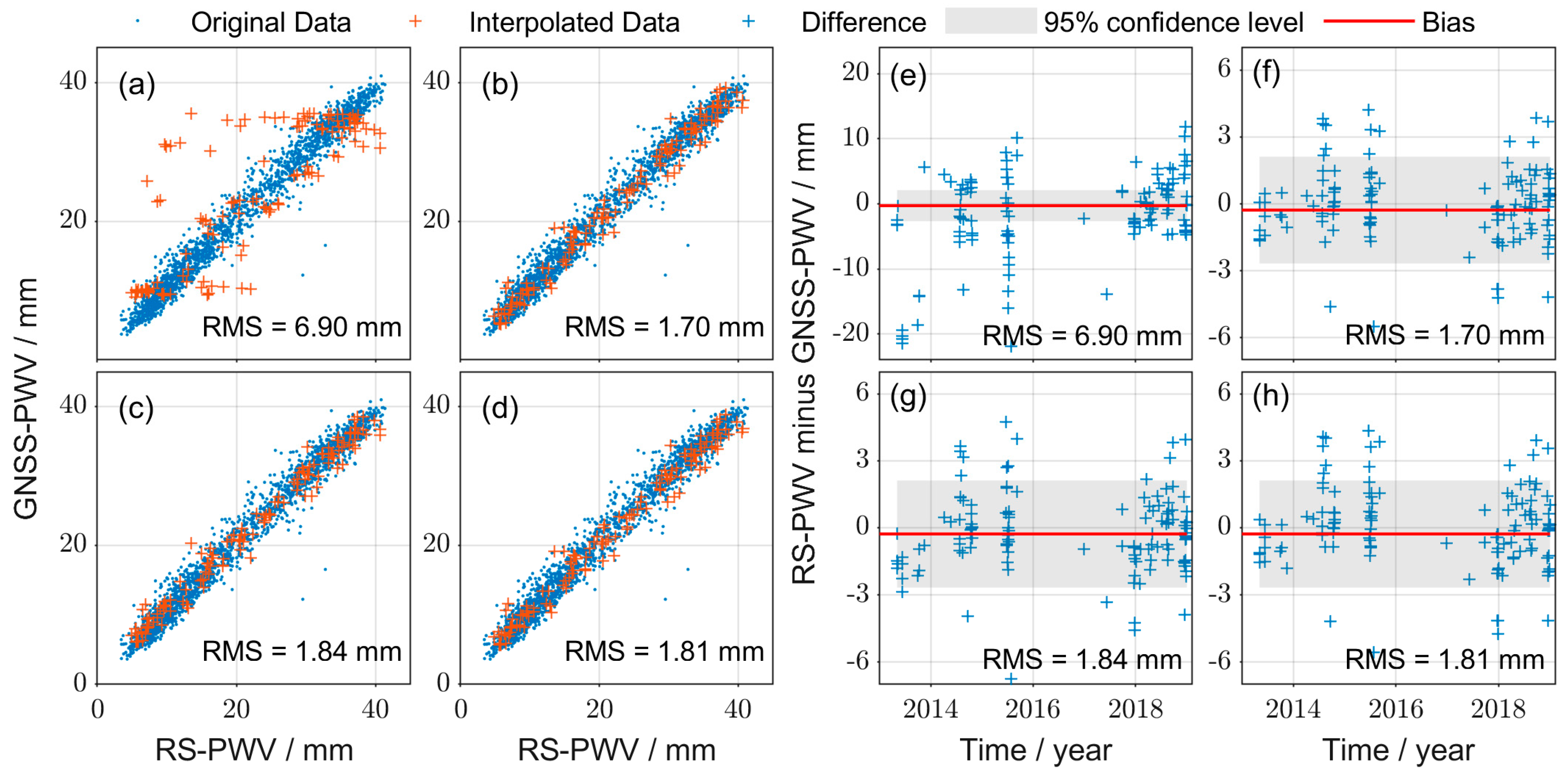
The ERA-PWV was simultaneously used as the data source for the interpolation and reference data for the last comparison, which may lead to questionable results. Therefore, independent RS-PWV were introduced as the reference for another comparison to further validate the performance of the IRDPCA. There are four radiosonde stations co-located with GNSS stations in the research area, but only one station (56778) could provide enough available observations in the study period. Therefore, RS-PWV over 56778 was set as the reference to compare the original and interpolated GNSS-PWV over KMIN from these four methods. Figure 14 shows the comparison results between GNSS-PWV and RS-PWV over KMIN. It is obvious that the RDPCA produced unsatisfactory interpolation results, containing some unexpected gross data. The interpolation data from the other three methods were much more consistent with the range of the original nonmissing data. The RMS values of the IRDPCA, DINEOF and IDW were 1.70, 1.84 and 1.81 mm, respectively, which were higher than the RMS of the original nonmissing GNSS-PWV (1.49 mm). The results also indicate the better performance of the IRDPCA among these methods. In addition, the IDW resulted in a higher RMS (1.81 mm) but did not significantly modify the agreement of the original GNSS-PWV in contrast to the last comparison based on the ERA-PWV. This also suggests that the IDW will introduce systematic biases in the interpolated data. The more convincing comparison based on the independent RS-PWV can further indicate that the IRDPCA outperformed the other interpolation methods based on the multisource PWV.

5. Discussion and Conclusions

GNSS-PWV is an important atmospheric parameter that is widely used in climatic analyses. An evenly sampled GNSS-PWV time series without any missing data is a prerequisite for most of the analyses. However, in practice, data gaps often occur, which is a common challenge for climatic applications. Most current studies focus on the interpolation for missing data only based on GNSS-PWV, but overlook the PWV obtained from other relatively independent techniques such as ERA-PWV. In this study, PCA-based interpolation methods were introduced to take care of the common spatiotemporal characteristic of GNSS-PWV and ERA-PWV. Then, how an initial guess of the missing data affected the final interpolation data was investigated theoretically, and a new PCA-based interpolation method, called IRDPCA, was proposed. By utilizing both the ERA-PWV and GNSS-PWV, the proposed IRDPCA method could interpolate the missing data well for the GNSS-PWV time series at the selected test GNSS stations without being affected by the systematic biases between the ERA-PWV and GNSS-PWV time series. The performance of the new method was compared with the RDPCA, DINEOF and IDW using experiments with ERA-PWV and GNSS-PWV data for a 6-year period at 26 GNSS stations in Yunnan Province, China, and good results were shown.
The experiments were conducted with various missing data rates for two cases: (1) interpolating ERA-PWV using ERA-PWV at surrounding grids for simulating a homogeneous case; (2) interpolating GNSS-PWV using ERA-PWV for simulating a heterogeneous case. The test results show that our new method can demonstrate great performance in the interpolation of missing data in both heterogeneous and homogeneous cases. The simulation test results also indicate that the performance of the IRDPCA was dependent upon the missing data rate in the heterogeneous data case. In addition, these four methods were used in the interpolation of real observed GNSS-PWV data series containing 26 stations’ GNSS-PWV time series with missing rates ranging from 3.3% to 24.6%. The results interpolated using all of the above four methods were compared against the original observed GNSS-PWV data series. The consistency between the original and interpolated data was then evaluated by comparing them with the reference ERA-PWV and RS-PWV for the same GNSS station. The results suggest that the IRDPCA can successfully perform the interpolation for missing data in heterogeneous GNSS-PWV time series and not be impacted by the potential systematic biases among multisource data. Since the excellent advantages of immunity to systematic biases, the IRDPCA can be safely used in the interpolation of missing data in different fields, such as GNSS station coordinate time series, meteorological observations from ground synoptic stations and water vapor data from remote sensing images.

Author Contributions

Conceptualization, D.Z., M.Z. and K.Z.; methodology, D.Z.; software, D.Z. and Z.Z.; validation, D.Z. and S.W.; formal analysis, D.Z. and Z.L.; investigation, D.Z.; resources, D.Z.; data curation, D.Z. and X.L.; writing—original draft preparation, D.Z.; writing—review and editing, D.Z., S.W. and J.L.; visualization, D.Z.; supervision, K.Z. and S.W.; project administration, K.Z. and Q.H.; funding acquisition, D.Z., K.Z. and Z.L. All authors have read and agreed to the published version of the manuscript.

Funding

This work was supported by the National Natural Science Foundations of China (No. 41730109, No. 42274021) and the State Key Laboratory of Geo-Information Engineering (No. SKLGIE2023-M-1-1).

Data Availability Statement

ERA5 reanalysis dataset and radiosonde observations can be freely available at https://www.ecmwf.int/en/forecasts/datasets (accessed on 15 September 2022) and https://www.ncei.noaa.gov/products/weather-balloon/integrated-global-radiosonde-archive (accessed on 19 October 2023). The authors do not have permission to share GNSS data.

Acknowledgments

The author would like to thank CMONOC, ECMWF and IGRA for providing highly precise GNSS ZTD products and atmospheric data.

Conflicts of Interest

The authors declare that they have no known competing financial interest or personal relationships that could have appeared to influence the work reported in this paper.

References

  1. Dessler, A.E.; Zhang, Z.; Yang, P. Water-vapor climate feedback inferred from climate fluctuations, 2003–2008. Geophys. Res. Lett. 2008, 35. [Google Scholar] [CrossRef]
  2. O’Gorman, P.A.; Muller, C.J. How closely do changes in surface and column water vapor follow Clausius–Clapeyron scaling in climate change simulations? Environ. Res. Lett. 2010, 5, 25207. [Google Scholar] [CrossRef]
  3. Patel, V.K.; Kuttippurath, J. Increase in Tropospheric Water Vapor Amplifies Global Warming and Climate Change. Ocean.-Land-Atmos. Res. 2023, 2, 15. [Google Scholar] [CrossRef]
  4. Solomon, S.; Rosenlof, K.H.; Portmann, R.W.; Daniel, J.S.; Davis, S.M.; Sanford, T.J.; Plattner, G. Contributions of Stratospheric Water Vapor to Decadal Changes in the Rate of Global Warming. Science 2010, 327, 1219–1223. [Google Scholar] [CrossRef]
  5. Antuña-Marrero, J.C.; Román, R.; Cachorro, V.E.; Mateos, D.; Toledano, C.; Calle, A.; Antuña-Sánchez, J.C.; Vaquero-Martínez, J.; Antón, M.; de Frutos Baraja, Á.M. Integrated water vapor over the Arctic: Comparison between radiosondes and sun photometer observations. Atmos. Res. 2022, 270, 106059. [Google Scholar] [CrossRef]
  6. Tan, J.; Chen, B.; Wang, W.; Yu, W.; Dai, W. Evaluating Precipitable Water Vapor Products from Fengyun-4A Meteorological Satellite Using Radiosonde, GNSS, and ERA5 Data. IEEE Trans. Geosci. Remote Sens. 2022, 60, 4106512. [Google Scholar] [CrossRef]
  7. Zhang, W.; Lou, Y.; Cao, Y.; Liang, H.; Shi, C.; Huang, J.; Liu, W.; Zhang, Y.; Fan, B. Corrections of Radiosonde-Based Precipitable Water Using Ground-Based GPS and Applications on Historical Radiosonde Data Over China. J. Geophys. Res. Atmos. 2019, 124, 3208–3222. [Google Scholar] [CrossRef]
  8. Ma, X.; Yao, Y.; Zhang, B.; Du, Z. FY-3A/MERSI precipitable water vapor reconstruction and calibration using multi-source observation data based on a generalized regression neural network. Atmos. Res. 2022, 265, 105893. [Google Scholar] [CrossRef]
  9. Ma, X.; Yao, Y.; Zhang, B.; Qin, Y.; Zhang, Q.; Zhu, H. An Improved MODIS NIR PWV Retrieval Algorithm Based on an Artificial Neural Network Considering the Land-Cover Types. IEEE Trans. Geosci. Remote Sens. 2022, 60, 5622412. [Google Scholar] [CrossRef]
  10. Lindenbergh, R.; Keshin, M.; van der Marel, H.; Hanssen, R. High resolution spatio-temporal water vapour mapping using GPS and MERIS observations. Int. J. Remote Sens. 2008, 29, 2393–2409. [Google Scholar] [CrossRef]
  11. Zhu, D.; Zhang, K.; Yang, L.; Wu, S.; Li, L. Evaluation and Calibration of MODIS Near-Infrared Precipitable Water Vapor over China Using GNSS Observations and ERA-5 Reanalysis Dataset. Remote Sens. 2021, 13, 2761. [Google Scholar] [CrossRef]
  12. Zhao, Q.; Du, Z.; Yao, W.; Yao, Y.; Li, Z.; Shi, Y.; Chen, L.; Liao, W. Precipitable water vapor fusion method based on artificial neural network. Adv. Space Res. 2022, 70, 85–95. [Google Scholar] [CrossRef]
  13. Vaquero-Martínez, J.; Antón, M.; Costa, M.J.; Bortoli, D.; Navas-Guzmán, F.; Alados-Arboledas, L. Microwave radiometer, sun-photometer and GNSS multi-comparison of integrated water vapor in Southwestern Europe. Atmos. Res. 2023, 287, 106698. [Google Scholar] [CrossRef]
  14. Bevis, M.; Businger, S.; Herring, T.A.; Rocken, C.; Anthes, R.A.; Ware, R.H. GPS meteorology: Remote sensing of atmospheric water vapor using the global positioning system. J. Geophys. Res. 1992, 97, 15787. [Google Scholar] [CrossRef]
  15. Hadas, T.; Teferle, F.N.; Kazmierski, K.; Hordyniec, P.; Bosy, J. Optimum stochastic modeling for GNSS tropospheric delay estimation in real-time. Gps Solut. 2017, 21, 1069–1081. [Google Scholar] [CrossRef]
  16. Sun, P.; Zhang, K.; Wu, S.; Wang, R.; Zhu, D.; Li, L. An investigation of a voxel-based atmospheric pressure and temperature model. Gps Solut. 2023, 27, 56. [Google Scholar] [CrossRef]
  17. Zhao, Q.; Liu, K.; Zhang, T.; He, L.; Shen, Z.; Xiong, S.; Shi, Y.; Chen, L.; Liao, W. A Global Conversion Factor Model for Mapping Zenith Total Delay onto Precipitable Water. Remote Sens. 2022, 14, 1086. [Google Scholar] [CrossRef]
  18. Lu, C.; Zhang, Y.; Zheng, Y.; Wu, Z.; Wang, Q. Precipitable water vapor fusion of MODIS and ERA5 based on convolutional neural network. Gps Solut. 2023, 27, 15. [Google Scholar] [CrossRef]
  19. Zhang, M.; Zhang, K.; Wu, S.; Shi, J.; Li, L.; Wu, H.; Liu, S. A new method for tropospheric tomography using GNSS and Fengyun-4A data. Atmos. Res. 2022, 280, 106460. [Google Scholar] [CrossRef]
  20. Zhao, Q.; Yao, Y.; Yao, W. GPS-based PWV for precipitation forecasting and its application to a typhoon event. J. Atmos. Sol.-Terr. Phys. 2018, 167, 124–133. [Google Scholar] [CrossRef]
  21. Zhu, L.; Yang, L.; Xu, Y.; Zhang, H.; Wu, Z.; Wang, Z. Independent Validation of Jason-2/3 and HY-2B Microwave Radiometers Using Chinese Coastal GNSS. IEEE Trans. Geosci. Remote Sens. 2022, 60, 1–11. [Google Scholar] [CrossRef]
  22. Wang, J.; Zhang, L.; Dai, A.; Van Hove, T.; Van Baelen, J. A near-global, 2-hourly data set of atmospheric precipitable water from ground-based GPS measurements. J. Geophys. Res. 2007, 112. [Google Scholar] [CrossRef]
  23. Wang, X.; Zhang, K.; Wu, S.; Li, Z.; Cheng, Y.; Li, L.; Yuan, H. The correlation between GNSS-derived precipitable water vapor and sea surface temperature and its responses to El Niño–Southern Oscillation. Remote Sens. Environ. 2018, 216, 1–12. [Google Scholar] [CrossRef]
  24. Alshawaf, F.; Zus, F.; Balidakis, K.; Deng, Z.; Hoseini, M.; Dick, G.; Wickert, J. On the Statistical Significance of Climatic Trends Estimated from GPS Tropospheric Time Series. J. Geophys. Res. Atmos. 2018, 123, 10967–10990. [Google Scholar] [CrossRef]
  25. Yang, F.; Guo, J.; Meng, X.; Shi, J.; Zhou, L. Establishment and Assessment of a New GNSS Precipitable Water Vapor Interpolation Scheme Based on the GPT2w Model. Remote Sens. 2019, 11, 1127. [Google Scholar] [CrossRef]
  26. Alshawaf, F.; Fersch, B.; Hinz, S.; Kunstmann, H.; Mayer, M.; Meyer, F.J. Water vapor mapping by fusing InSAR and GNSS remote sensing data and atmospheric simulations. Hydrol. Earth Syst. Sci. 2015, 19, 4747–4764. [Google Scholar] [CrossRef]
  27. Xu, W.B.; Li, Z.W.; Ding, X.L.; Zhu, J.J. Interpolating atmospheric water vapor delay by incorporating terrain elevation information. J. Geod. 2011, 85, 555–564. [Google Scholar] [CrossRef]
  28. Hersbach, H.; Bell, B.; Berrisford, P.; Hirahara, S.; Horányi, A.; Muñoz Sabater, J.; Nicolas, J.; Peubey, C.; Radu, R.; Schepers, D.; et al. The ERA5 global reanalysis. Q. J. R. Meteorol. Soc. 2020, 146, 1999–2049. [Google Scholar] [CrossRef]
  29. Shum, H.Y.; Ikeuchi, K.; Reddy, R. Principal component analysis with missing data and its application to polyhedral object modeling. IEEE Trans. Pattern Anal. Mach. Intell. 1995, 17, 854–867. [Google Scholar] [CrossRef]
  30. Beckers, J.M.; Rixen, M. EOF calculations and data filling from incomplete oceanographic datasets. J. Atmos. Ocean. Technol. 2003, 20, 1839–1856. [Google Scholar] [CrossRef]
  31. Taylor, M.H.; Losch, M.; Wenzel, M.; Schröter, J. On the Sensitivity of Field Reconstruction and Prediction Using Empirical Orthogonal Functions Derived from Gappy Data. J. Clim. 2013, 26, 9194–9205. [Google Scholar] [CrossRef]
  32. Ping, B.; Su, F.; Meng, Y. Reconstruction of Satellite-Derived Sea Surface Temperature Data Based on an Improved DINEOF Algorithm. IEEE J. Sel. Top. Appl. Earth Observ. Remote Sens. 2015, 8, 4181–4188. [Google Scholar] [CrossRef]
  33. Shen, Y.; Peng, F.; Li, B. Improved singular spectrum analysis for time series with missing data. Nonlinear Process Geophys. 2015, 22, 371–376. [Google Scholar] [CrossRef]
  34. Shen, Y.; Li, W.; Xu, G.; Li, B. Spatiotemporal filtering of regional GNSS network’s position time series with missing data using principle component analysis. J. Geod. 2014, 88, 1–12. [Google Scholar] [CrossRef]
  35. He, X.; Yu, K.; Montillet, J.; Xiong, C.; Lu, T.; Zhou, S.; Ma, X.; Cui, H.; Ming, F. GNSS-TS-NRS: An Open-Source MATLAB-Based GNSS Time Series Noise Reduction Software. Remote Sens. 2020, 12, 3532. [Google Scholar] [CrossRef]
  36. He, X.; Hua, X.; Yu, K.; Xuan, W.; Lu, T.; Zhang, W.; Chen, X. Accuracy enhancement of GPS time series using principal component analysis and block spatial filtering. Adv. Space Res. 2015, 55, 1316–1327. [Google Scholar] [CrossRef]
  37. Dong, D.; Fang, P.; Bock, Y.; Webb, F.; Prawirodirdjo, L.; Kedar, S.; Jamason, P. Spatiotemporal filtering using principal component analysis and Karhunen-Loeve expansion approaches for regional GPS network analysis. J. Geophys. Res. Solid Earth 2006, 111. [Google Scholar] [CrossRef]
  38. Serneels, S.; Verdonck, T. Principal component analysis for data containing outliers and missing elements. Comput. Stat. Data Anal. 2008, 52, 1712–1727. [Google Scholar] [CrossRef]
  39. Alvera-Azcárate, A.; Barth, A.; Rixen, M.; Beckers, J.M. Reconstruction of incomplete oceanographic data sets using empirical orthogonal functions: Application to the Adriatic Sea surface temperature. Ocean. Model. 2005, 9, 325–346. [Google Scholar] [CrossRef]
  40. Saastamoinen, J. Atmospheric Correction for the Troposphere and Stratosphere in Radio Ranging Satellites. In The Use of Artificial Satellites for Geodesy; Wiley Online Library: Hoboken, NJ, USA, 2013; Volume 15, pp. 247–251. [Google Scholar] [CrossRef]
  41. Zhu, D.; Zhang, K.; Sun, P.; Wu, S.; Wan, M. Homogenization of daily precipitable water vapor time series derived from GNSS observations over China. Adv. Space Res. 2023, 72, 1751–1763. [Google Scholar] [CrossRef]
  42. Zhu, D.; Zhang, K.; Shen, Z.; Wu, S.; Liu, Z.; Tong, L. A New Adaptive Absolute Method for Homogenizing GNSS-Derived Precipitable Water Vapor Time Series. Earth Space Sci. 2021, 8, e2021EA001716. [Google Scholar] [CrossRef]
  43. Bock, O.; Bosser, P.; Mears, C. An improved vertical correction method for the inter-comparison and inter-validation of integrated water vapour measurements. Atmos. Meas. Tech. 2022, 15, 5643–5665. [Google Scholar] [CrossRef]
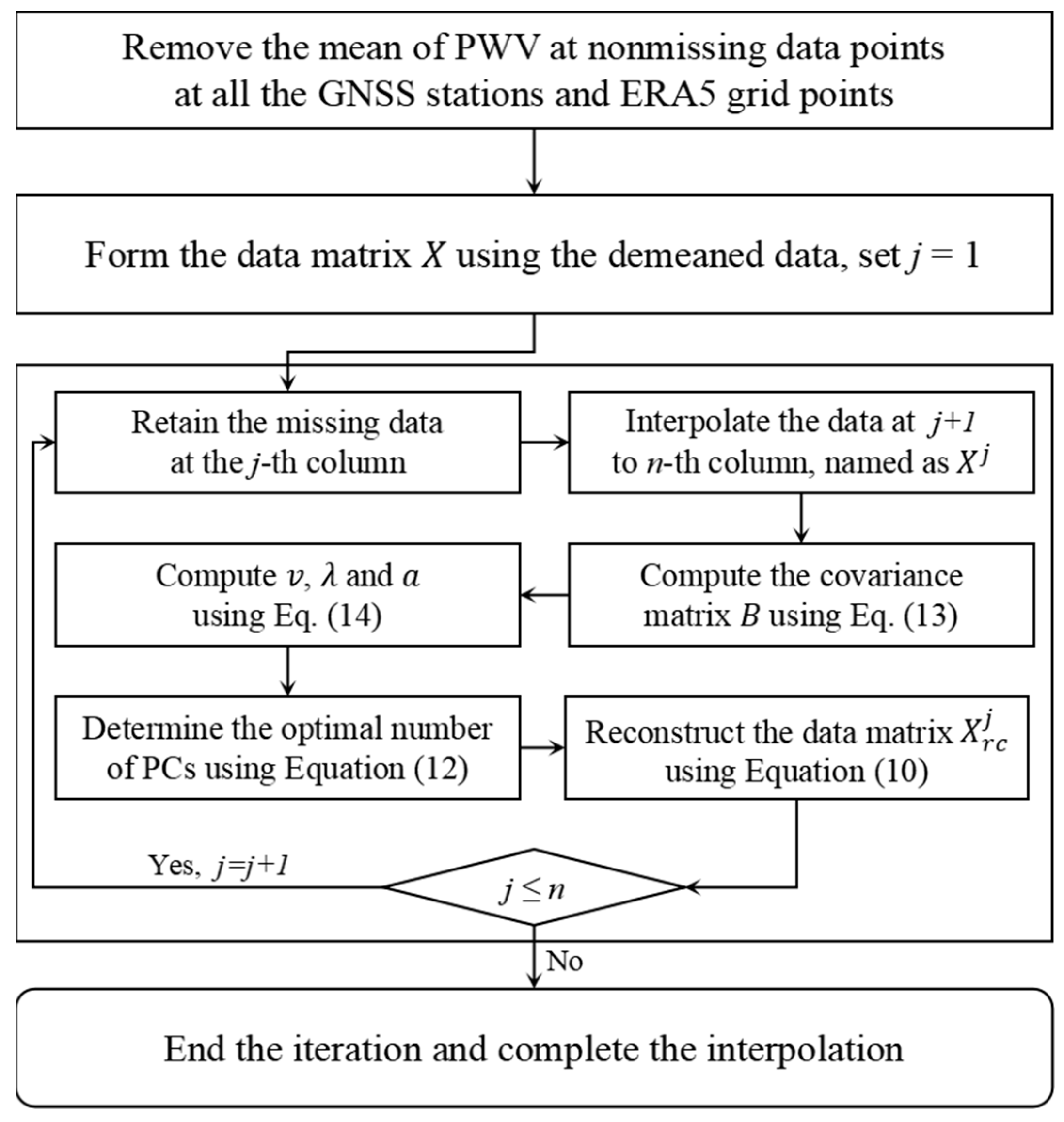
Figure 1. Flowchart of the IRDPCA for the interpolation process.
Remotesensing 15 05153 g001
Figure 2. (a) Missing data rate and (b) annual mean PWV value at the selected 26 GNSS stations.
Remotesensing 15 05153 g002
Figure 3. Data availability (top) and missing data rate (bottom) at each of the selected 26 GNSS stations.
Remotesensing 15 05153 g003
Figure 4. Spatial distribution of the ERA5 gird points used in the simulation.
Remotesensing 15 05153 g004
Figure 5. (a) RMS of the interpolation error and (b) reconstruction error from various missing rates.
Remotesensing 15 05153 g005
Figure 6. (a) RMS and (b) bias of the first largest eigenvalue of the interpolated PWV relative to the true values of the original nonmissing PWV.
Remotesensing 15 05153 g006
Figure 7. (a) RMS and (b) bias of the second largest eigenvalue of the interpolated PWV relative to the true values of the original nonmissing PWV.
Remotesensing 15 05153 g007
Figure 8. (a) RMS of interpolation error and (b) reconstruction error resulting from simulated GNSS-PWV at various missing rates and four methods.
Remotesensing 15 05153 g008
Figure 9. Seasonal RMS of the interpolation errors resulting from each missing rate and method: (a) RDPCA; (b) IRDPCA; (c) DINEOF; (d) IDW. The spring, summer, autumn and winter seasons are defined as December–January–February, March–April–May, June–July–August and September–October–November, respectively.
Remotesensing 15 05153 g009
Figure 10. RMS of the interpolation errors at each GNSS station resulting from the interpolation method: (a) RDPCA; (b) IRDPCA; (c) DINEOF; (d) IDW.
Remotesensing 15 05153 g010
Figure 11. RMS (upper), absolute bias (middle) and correlation coefficient (bottom) between the GNSS-PWV interpolated from each method and the reference ERA-PWV interpolated for each station. The original data (see the labels on the top) indicate the same three statistical results between the original GNSS-PWV and reference ERA-PWV at all nonmissing data points.
Remotesensing 15 05153 g011
Figure 12. Interpolated GNSS-PWV and the difference between the interpolated GNSS-PWV and the reference ERA-PWV at missing data points at the YNHZ station during the 6-year period from 2013 to 2018: (a,e) RDPCA; (b,f) IRDPCA; (c,g) DINEOF; (d,h) IDW. The red lines and the shaded areas represent the bias and 95% confidence interval derived from the RMS value (2.79 mm) based on the nonmissing GNSS-PWV and ERA-PWV.
Remotesensing 15 05153 g012
Figure 13. Six-year GNSS-PWV time series from the original observations (red) and interpolation (blue) using (a) RDPCA; (b) IRDPCA; (c) DINEOF; (d) IDW.
Remotesensing 15 05153 g013
Figure 14. Interpolated GNSS-PWV and the difference between the interpolated GNSS-PWV and the reference RS-PWV at missing data points at the KMIN station during the 6-year period from 2013 to 2018: (a,e) RDPCA; (b,f) IRDPCA; (c,g) DINEOF; (d,h) IDW.
Remotesensing 15 05153 g014
Disclaimer/Publisher’s Note: The statements, opinions and data contained in all publications are solely those of the individual author(s) and contributor(s) and not of MDPI and/or the editor(s). MDPI and/or the editor(s) disclaim responsibility for any injury to people or property resulting from any ideas, methods, instructions or products referred to in the content.