Rangeland Brush Estimation Tool (RaBET): An Operational Remote Sensing-Based Application for Quantifying Woody Cover on Western Rangelands

Abstract

Much of the western United States is covered by rangelands used for grazing and wildlife. Woody plant cover is increasing in areas historically covered by grasslands and can cause numerous problems, including losses in wildlife habitat, forage for grazing, and overall losses in soil health. Land managers and conservationists are working to control these increases in woody plants, but need tools to help determine target areas to focus efforts and resources where they are most needed. In this work, we present RaBET (Rangeland Brush Estimation Tool), which uses transparent, well-understood methodologies with remotely sensed data to map woody canopy cover across large areas of rangelands. We demonstrate that our process produced more accurate results than two currently available tools based on advanced machine learning techniques. We compare two methods of map validation: traditional field methods of plant canopy measurements; and aircraft-based photography, which decreases the amount of time and resources needed. RaBET is a remote sensing-based application for obtaining repeatable, accurate measures of woody cover to aid land managers and conservationists in the control of woody plants on rangelands.

1. Introduction

Woody plant encroachment in rangelands is one of the challenges that ranchers, land managers, and conservationists have faced for decades [1,2]. Left unchecked, increases in woody species can cause the loss of native perennial grasses and lead to declines in forage availability, biodiversity, wildlife habitat, and soil health, ultimately leading to loss of function and services throughout rangeland ecosystems [3,4,5].

Implementing conservation practices through informed management is critical for ensuring the health and sustainability of natural resources throughout rangelands and other ecosystems. Brush management as a conservation practice includes the treatment of woody plants with a variety of methods, including herbicides, prescribed fire, and mechanical removal to mitigate decreases in system function [6,7]. Efficacy, sustainability, and cost of conservation practices depend on timing, location, and treatment method(s); thus, significant planning is necessary [8]. Monitoring and accurately assessing treatment outcomes poses a substantial challenge, particularly when dealing with vast expanses of land with limited resources [9,10,11].

Numerous federal and state government agencies and non-governmental organizations have adopted brush management in rangeland ecosystems [12]. The United States Department of Agriculture’s Natural Resources Conservation Service (NRCS), for example, spends millions of dollars each year on brush management through the Environmental Quality Incentives Program (EQIP), which provides financial support to ranchers and other agricultural producers to identify and use appropriate conservation practices [13].

The NRCS Conservation Effects Assessment Project (CEAP) examines the impact of conservation practices on natural resources such as soil, water, and wildlife [14]. The project’s goal is to give decision-makers and policymakers science-based information to help evaluate conservation practices, prioritize funding, and allocate resources where they are most needed. The processes of monitoring and evaluating a conservation practice can be constrained by the availability of sufficient personnel to conduct field surveys during time-sensitive periods. Data collection is thus limited to key areas that are unlikely to capture the variability in spatial or spectral characteristics of larger landscapes due to topography and soils as well as temporal impacts arising with changing climate and land use.

Remote sensing-based methods have been developed, often incorporating ground-based data, to map rangeland vegetation [15,16,17,18,19,20]. Many of these maps are restricted by vegetation type, have limited spatial coverage, and/or only provide snapshots in time [15,16,17,18]; this does not meet brush management needs for planning and documenting changes in time and space over a variety of landscapes. The Rangeland Analysis Platform (RAP) and Landscape Cover Analysis and Reporting Tool (LandCART) quantify woody or brush cover from satellite imagery, provide time series maps, and are currently available for the assessment and monitoring at regional/national scales [19,20]. However, neither tool is optimized for rangelands. Woody canopy cover values at ranch or pasture scales that capture rangeland landscape variability are more useful for the planning, implementation, and monitoring of brush management.

In this work, we present RaBET (Rangeland Brush Estimation Tool), which provides maps of woody canopy cover and uses transparent, well-understood methodologies with remotely sensed data and parameters tuned to rangelands in Major Land Resource Areas (MLRAs) [21] ranging in area up to 145,000 sq. km. Our primary goal is to compare RaBET output with RAP and LandCART, which use advanced machine learning techniques, and demonstrate that our process produces more accurate results. In addition, we compare two methods of map validation, traditional field methods of plant canopy measurements and aircraft-based photography, to explore the disconnect that often exists between ground-based and remotely sensed vegetation observations.

2. Materials and Methods

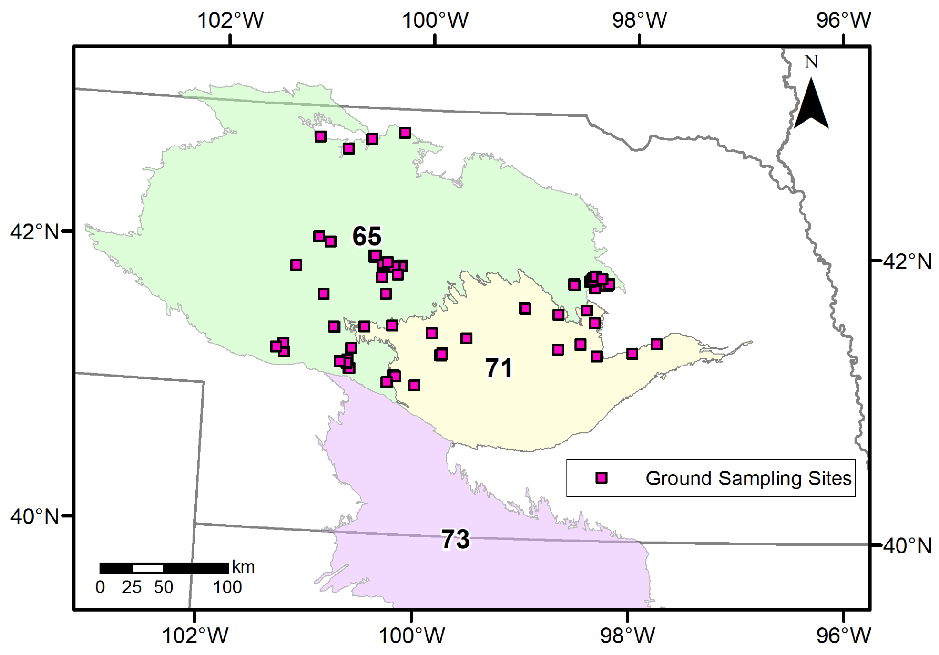
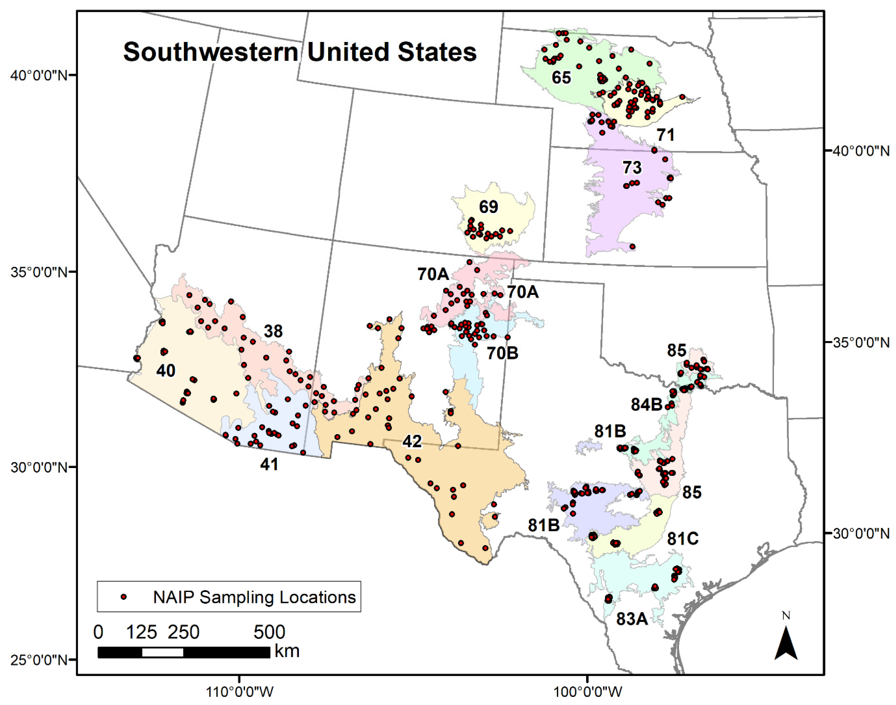
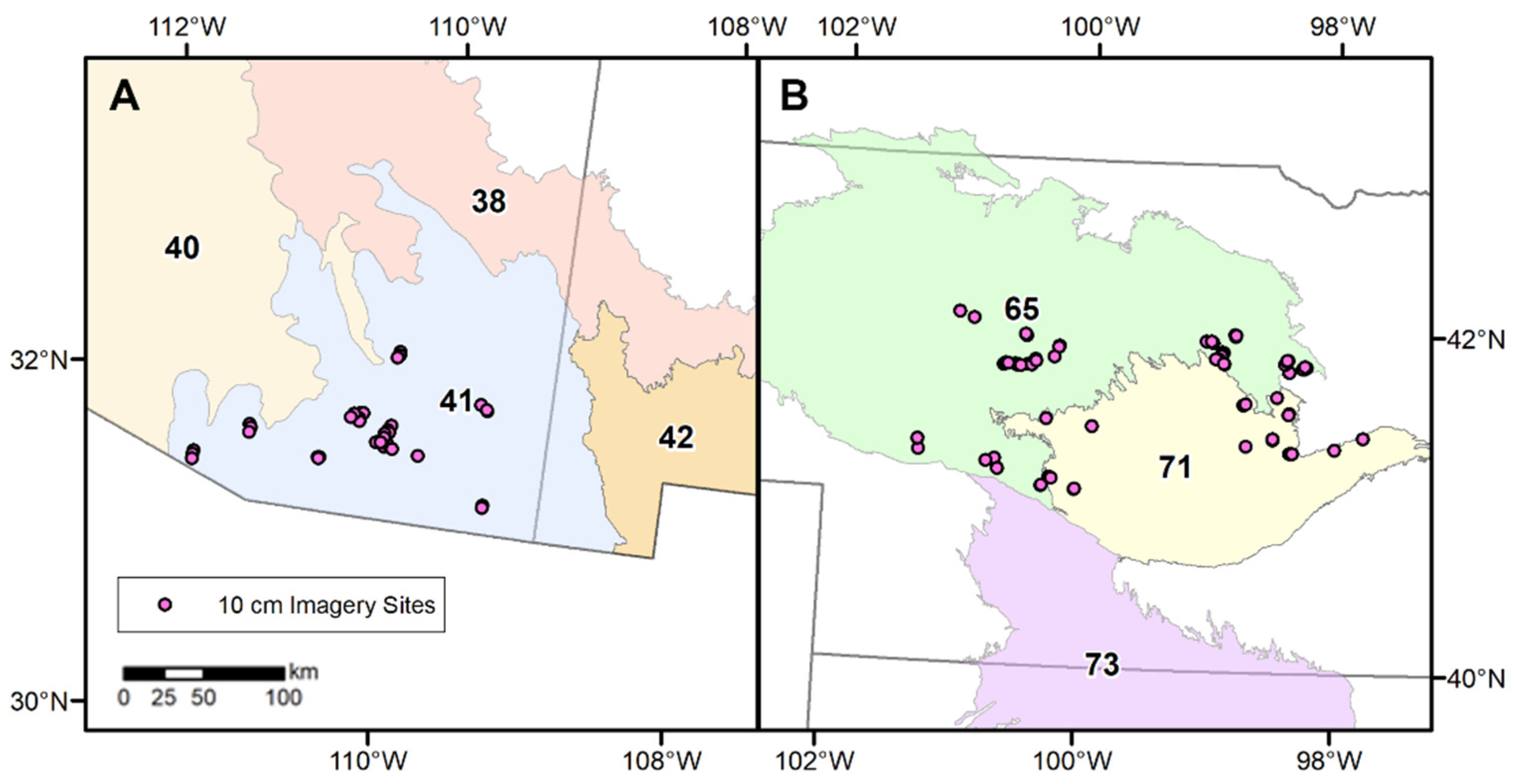
2.1. Study Areas

This work was conducted within 15 Major Land Resource Areas (MLRAs) across the western United States (Figure 1) [21]. MLRAs are large areas characterized by similar patterns of soils, climate, water resources, and land uses, which are important for agricultural planning at regional and national scales [21]. Study MLRAs extend from Arizona east to Texas and north to Nebraska. Elevations ranged from 60 m in Texas to approximately 2285 m in the mountains of Arizona, with vegetation spanning desert scrubland, savannas and prairies, and dense forests. Some of the most common woody species present include pinyon (Pinus spp.), juniper (Juniperus communis L.), eastern redcedar (Juniperus virginiana L.), and mesquite (Prosopis spp.), which are often targets for removal through brush management. MLRA sizes ranged widely from 15,970 sq. km up to 145,040 sq. km with annual average precipitation of 75 to 1065 mm and annual air temperatures of 8 to 23 °C (

Table 1. Major Land Resource Area descriptions of symbol, location, size, name, average annual precipitation, and average annual air temperature [21].

MLRA Symbol	State(s)	Size (sq. km)	MLRA Name	Avg. Annual Precip. (mm)	Avg. Annual Air Temp. (°C)
38	AZ NM	49,195	Mogollon Transition	255 to 940	8 to 21
40	AZ	82,310	Sonoran Basin and Range	75 to 255	15 to 23
41	AZ	40,765	Southeastern Arizona Basin and Range	230 to 510	8 to 20
42	NM TX	145,040	Southern Desertic Basins, Plains, and Mountains	205 to 355	10 to 22
65	NE	53,235	Nebraska Sand Hills	380 to 660	8 to 10
69	CO	30,885	Upper Arkansas Valley Rolling Plains	255 to 485	8 to 12
70A	NM	27,910	Canadian River Plains and Valleys	255 to 535	8 to 14
70B	NM	25,660	Upper Pecos River Valley	330 to 380	12 to 16
71	NE	21,160	Central Nebraska Loess Hills	535 to 735	8 to 11
73	NE KS	55,670	Rolling Plains and Breaks	485 to 760	9 to 14
81B	TX	28,825	Edwards Plateau, Central Part	485 to 815	17 to 20
81C	TX	20,890	Edwards Plateau, Eastern Part	610 to 760	17 to 20
83A	TX	28,805	Northern Rio Grande Plain	535 to 940	20 to 22
84B	TX OK	15,970	West Cross Timbers	660 to 1065	17 to 19
85	TX OK	26,955	Grand Prairie	685 to 1040	16 to 19

).

2.2. Data

The following subsections describe the data sources and methods used for this work. A schematic of how the datasets and methods relate is provided in Figure 2. Landsat satellite imagery and National Agriculture Imagery Program (NAIP) aerial orthophotography were used to create vegetation indices and linear regressions. The regressions were applied to Landsat vegetation indices to create RaBET maps. National Land Cover Database (NLCD) layers were applied to the RaBET maps to mask out unwanted features. RaBET maps were validated using NAIP, finer resolution (10 cm) aerial imagery, and ground-based data. Comparisons of RaBET maps and RAP and LandCART map products were performed.

2.2.1. Aerial Orthophotography

High-resolution imagery was used for map creation and validation. Subsets of National Agriculture Imagery Program (NAIP) imagery at 0.6 m resolution were used as samples from each MLRA (

Table 2. Major Land Resource Areas: state locations, image type, and year.

MLRA	State(s)	Image Type	Image Year
38	AZ NM	NAIP NAIP	2018 2016
40	AZ	NAIP	2019
41	AZ	NAIP 10 cm	2019 2022
42	NM TX	NAIP NAIP	2018 2016
65	NE	NAIP 10 cm	2016, 2018 2020
69	CO	NAIP	2018
70A	NM	NAIP	2018
70B	NM	NAIP	2018
71	NE	NAIP 10 cm	2018 2022
73	NE KS	NAIP NAIP	2018 2019
81B	TX	NAIP	2020
81C	TX	NAIP	2020
83A	TX	NAIP	2020
84B	TX OK	NAIP NAIP	2020 2019, 2020
85	TX OK	NAIP NAIP	2020 2019

). Samples were collected via the Google Earth Engine (GEE) repository and classified into woody and non-woody classes using the Support Vector Machine supervised classification method [22] in ArcGIS Pro. Approximate extents of classified pasture-sized samples ranged between 400 m × 400 m and 900 m × 900 m. There were between 18 and 46 samples per MLRA. Accuracy of each classified sample was determined using a stratified random Kappa Coefficient test [23]. Samples failing to meet a 0.7 Kappa threshold were excluded.

Privately contracted finer spatial resolution (10 cm) orthoimagery was also collected for MLRAs 41, 65, and 71 (Table 2, Figure 3). Pasture-sized imagery sites were overlaid with polylines to create sampling block layouts composed of one 100 m baseline and six 70 m side lines. At 0.5 m intervals, line-point intercepts (woody, non-woody) were read directly from the imagery to calculate woody canopy cover for validation of woody cover maps.

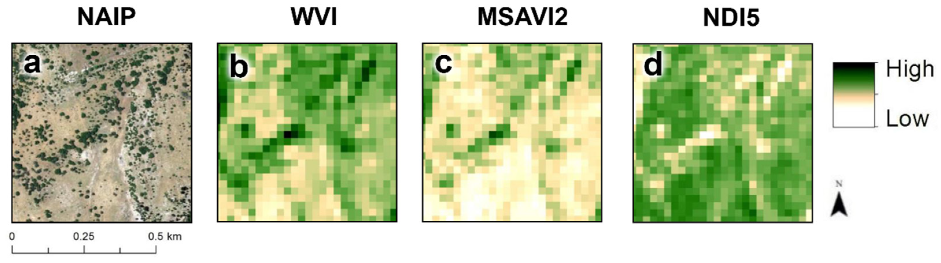
2.2.2. Landsat Satellite Imagery

Collection 1 Landsat 5 Thematic Mapper (TM), Landsat 7 Enhanced Thematic Mapper Plus (ETM+), and Landsat 8 Operational Land Imager (OLI) Level 2 Surface Reflectance products, courtesy of the U.S. Geological Survey, were used for woody cover map development. Cloud cover screening was performed and images with cloud cover thresholds above 10% were excluded.

For this work, the temporal range of the data used was 2015–2021. Rather than using the full 12-month time series per year, as is common when using vegetation indices [19,24,25,26,27], the months used here were based on phenology time windows appropriate for the MLRA’s woody species targeted for management and are shown in

Table 3. Major Land Resource Areas: state locations and Landsat phenology window.

MLRA	State(s)	Landsat Phenology Window
38	AZ NM	Jan, Feb, Mar
40	AZ	Mar, Apr
41	AZ	Jun
42	NM TX	Apr, May
65	NE	Jan, Feb, Mar, Apr, Nov, Dec
69	CO	Jan, Feb, Mar, Nov, Dec
70A	NM	Jan, Feb, Mar, Nov, Dec
70B	NM	Jan, Feb, Mar, Nov, Dec
71	NE	Jan, Feb, Mar, Nov, Dec
73	NE KS	Jan, Feb, Mar, Nov, Dec Jan, Feb, Mar
81B	TX	Jan, Feb, Mar, Dec
81C	TX	Jan, Dec
83A	TX	Jan, Dec
84B	TX OK	May, Jun, Jul, Aug
85	TX OK	May, Jun, Jul, Aug

. Phenology windows were periods of time when, ideally, the woody target species of interest for brush management would be green and background vegetation would not. Maps available in the final RaBET web application used Landsat data from 1997–2021 with the phenology windows shown in Table 3.

Three Landsat-based vegetation indices were used for this work. The Woody Vegetation Index (WVI) is a new index developed for RaBET, based on the “Green” NDVI [28] and the Soil Adjusted Total Vegetation Index (SATVI) [29,30], which emphasizes woody vegetation,

$$\mathrm{WVI}=\frac{\rho \mathrm{NIR}-\rho \mathrm{GREEN}}{\rho \mathrm{NIR}+\rho \mathrm{GREEN}}-\frac{\rho \mathrm{SWIR}1}{2}$$

(1)

where $\rho \mathrm{NIR}, \rho \mathrm{GREEN}$, and $\rho \mathrm{SWIR}1$ are near-infrared (NIR), green, and shortwave infrared (SWIR) reflectance, respectively. Utilizing the green rather than red reflectance normally used with NDVI provides higher sensitivity to chlorophyll concentration [28]. The Modified Soil Adjusted Vegetation Index (MSAVI2) [31,32],

$$\mathrm{MSAVI}2=\frac{2\rho \mathrm{NIR}\pm 1-\sqrt{{(2\rho \mathrm{NIR}+1)}^2-8(\rho \mathrm{NIR}-\rho \mathrm{RED})}}{2}$$

(2)

where $\rho \mathrm{RED}$ is red reflectance, was used to minimize the effects of variable soil background in heterogeneous areas. The Normalized Difference Index 5 (NDI5) [33,34],

$$\mathrm{NDI}5=\frac{\rho \mathrm{NIR}-\rho \mathrm{SWIR}1}{\rho \mathrm{NIR}+\rho \mathrm{SWIR}1}$$

(3)

was originally developed to detect crop residue. In this case, it was used to highlight dry herbaceous standing biomass, like senescent grasses. Figure 4 demonstrates different aspects of detection by the three indices in comparison with a reference natural color NAIP sample of the same area. WVI captures all of the woody areas, but also background grass and soil signals. MSAVI2 removes the grass and soil background, but also loses a portion of woody vegetation. NDI5 functions in the opposite manner than the other indices, with grasses being highlighted and woody vegetation removed. When used in combination, a stronger signal for woody vegetation is possible.

2.2.3. National Land Cover Database (NLCD)

The National Land Cover Database (NLCD) land cover product covers the conterminous United States of America and is maintained and updated periodically by the Multi-Resolution Land Characteristics Consortium that is composed of several federal agencies (https://www.mrlc.gov/, accessed on 24 March 2017 and 5 January 2022; https://www.mrlc.gov/data, accessed on 24 March 2017 and 5 January 2022). The NLCD product includes a suite of land cover maps for periods between 2001 to 2021 at varying time intervals and uses a 30 m Landsat-compatible pixel size. RaBET maps were masked using modifications to the 2016 NLCD map for all MLRAs except for the MLRA 65 mask, which was based on the 2019 NLCD map. Excluded NLCD classes were open water, perennial ice/snow, developed, barren land, pasture/hay, and cultivated crops. Included NLCD classes were forest types, scrub types, grassland/herbaceous, and woody and emergent herbaceous wetlands. Barren land was included for MLRA 40 only.

2.2.4. Rangeland Analysis Platform (RAP)

RAP is a vegetation cover product that utilizes aggregated NRCS National Resource Inventory (NRI) and Bureau of Land Management (BLM) Assessment, Inventory, and Management (AIM) field data with remote sensing products to generate fractional cover maps [19]. These data were aggregated into annual forbs and grasses, perennial forbs and grasses, shrubs, trees, litter, and bare ground functional cover types. The field data and Landsat 5 TM, 7 ETM+, and 8 OLI surface reflectance products were used in an Artificial Neural Network (ANN) to produce fractional cover maps of the six cover types. The 2018–2021 tree cover maps from RAP version 3 were used for this work.

2.2.5. Landscape Cover Analysis and Reporting Tool (LandCART)

LandCART is a web-based mapping tool that can be used to generate and download fractional cover maps of selected BLM AIM indicators (e.g., annual and perennial forbs and grasses, bare ground, canopy gaps, sagebrush, succulents, and trees) and display histograms of their distribution [20]. LandCART uses AIM, NRI and National Park Service (NPS) field data, Landsat 5 TM, 7 ETM+, and 8 OLI imagery, GEE, and Random Forest machine learning techniques to generate its fractional cover maps [35,36]. The 2018–2021 tree cover maps were used for this work.

2.2.6. Ground Data

Field campaigns were conducted in MLRAs 65 and 71 to collect ground-based data for validation checks (Figure 5). Sampling sites were composed of seven transect lines, one 100 m baseline with six 70 m side lines (three on each side of the baseline, spaced at 15 m intervals along the length of the baseline). A combination of line-point intercept and belt transect methods [37] were used to estimate woody canopy and ground cover. Observations at 0.5 m intervals were recorded for canopy and ground hits. Woody species that did not fall on the line but were within 3 m on either side of the transect were recorded as if present on the transect line. The ground hit was always recorded at the location on the transect line. All woody vegetation was recorded by species, and all other vegetation was recorded by lifeform. Readings were collected for 54 sites from October–November 2019 in MLRA 65. In MLRA 71, there were 23 sites collected over the span of December 2020, October–December 2021, and January 2022. All transect data were entered into the Vegetation GIS Data System (VGS) (https://vgs.arizona.edu, accessed on 1 October 2019), a suite of software applications for recording, managing, and using vegetation and other ecosystem related data, and woody canopy cover was calculated.

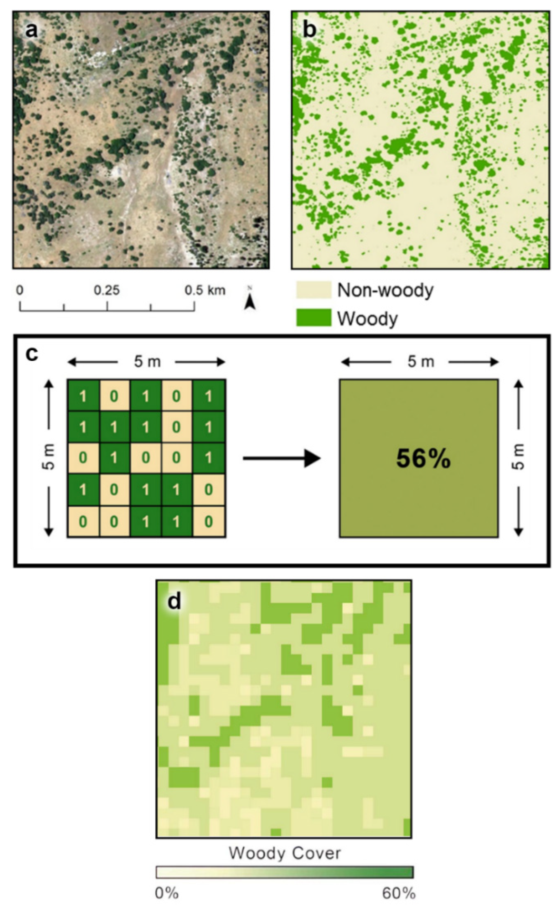
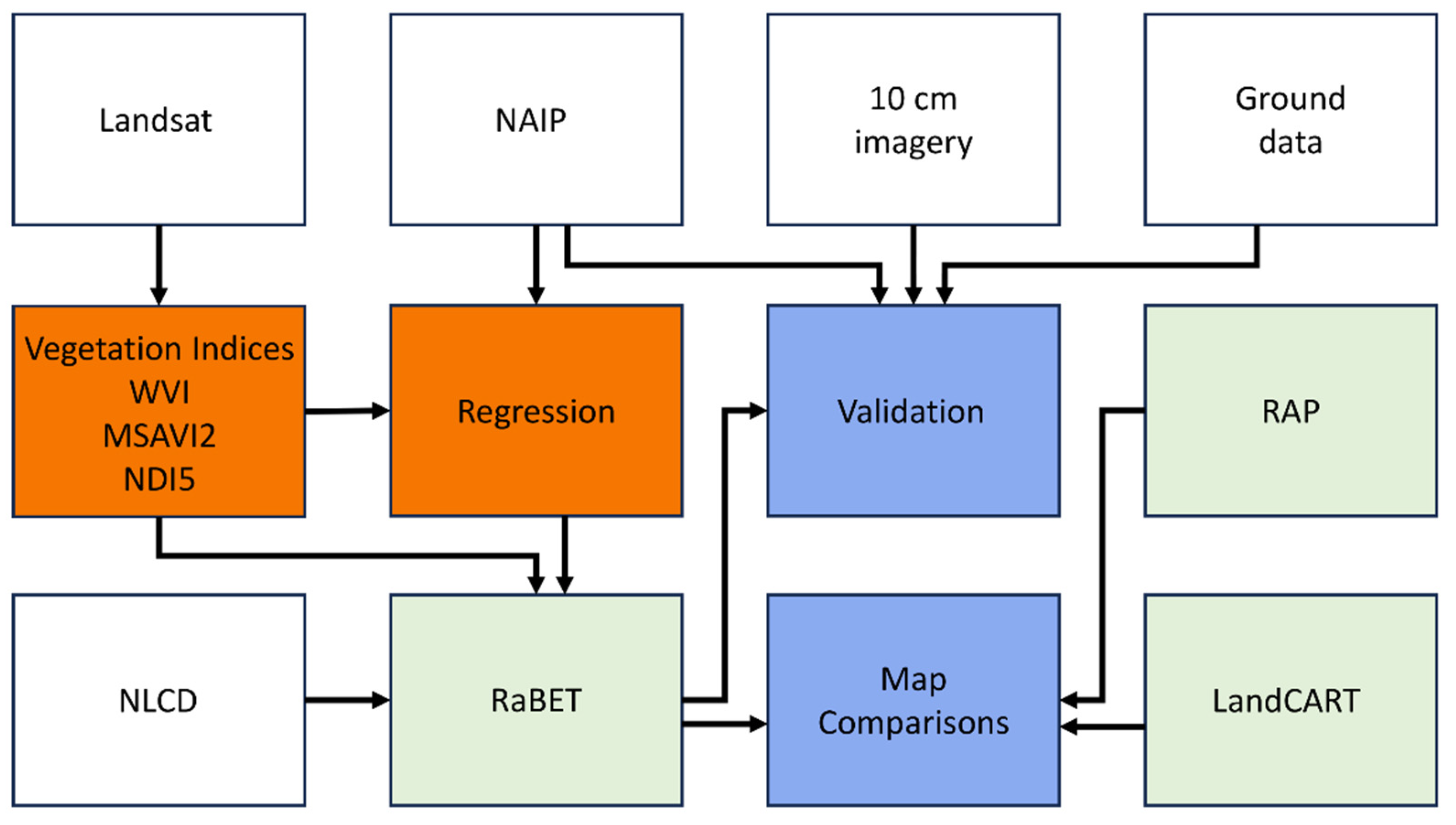
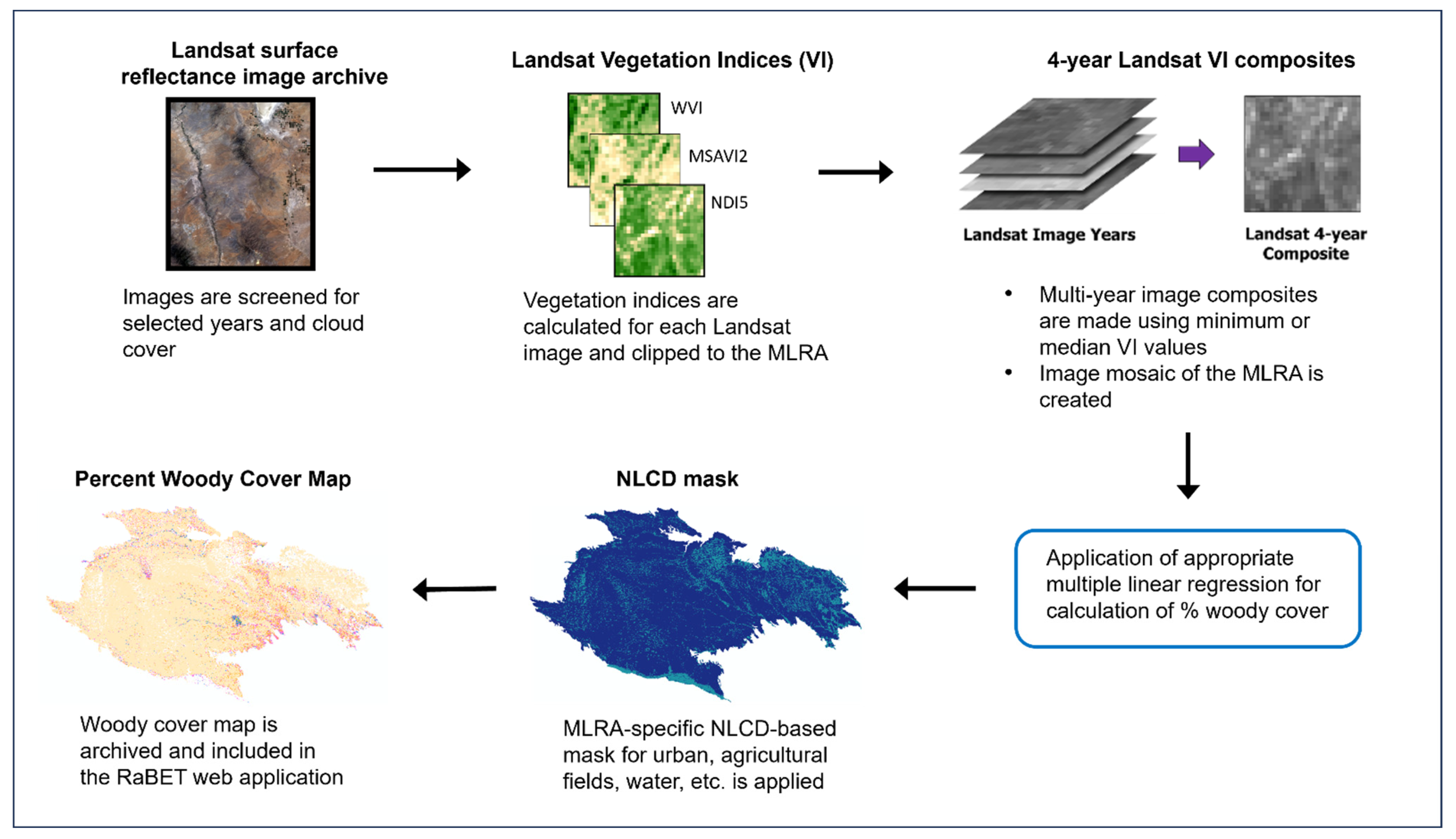
2.3. RaBET Woody Canopy Cover Map Generation

RaBET woody canopy cover maps were generated individually for each MLRA through a multistage process that included the aggregation of classified NAIP imagery (Figure 6) and the workflow for producing the maps (Figure 7). The aggregation step took the 0.6 m NAIP sample pixels that had been classified as woody (value = 1) and non-woody (value = 0) (Figure 6a,b) and applied the process described in Holifield Collins et al. [38]. Each classified image was reduced from native resolution using an aggregation function that set up an output image of 30 m pixel size corresponding to Landsat pixel locations. The function then summed woody cover pixels within each complete 30 m input image block to the matching output location (Figure 6c) to produce a 30 m NAIP-based woody cover image sample (Figure 6d). These 30 m samples were used to develop multiple linear regression coefficients for producing MLRA-specific woody canopy cover maps (

Table 4. Multiple linear regression coefficients calculated for the three vegetation indices (WVI, MSAVI, NDI5), Mean Absolute Error (MAE) for the regression, and the R squared value of the validation for each MLRA.

MLRA	State(s)	βWVI	βMSAVI2	βNDI5	β0	MAE	R2
38	AZ NM	167.95 270.74	98.86 −296.32	155.79 74.39	−44.01 −11.58	4.60 4.32	0.87 0.44
40	AZ	−19.82	227.55	−58.75	−0.23	4.63	0.30
41	AZ	67.93	198.83	−100.78	−6.48	5.32	0.76
42	NM TX	256.36	−539.26	−149.27	58.45	8.18	0.43
65	NE	121.39 243.10	52.82 −114.39	−51.39 52.79	−15.63 −51.02	2.27	0.95
69	CO	56.42	81.44	−22.25	−6.50	2.53	0.66
70A	NM	110.01	189.14	68.10	−43.44	4.73	0.54
70B	NM	160.92	189.81	−23.43	−48.87	3.46	0.74
71	NE	123.44	−268.90	−137.88	40.06	2.26	0.98
73	NE KS	271.28	−43.44	104.75	−79.56	6.59	0.54
81B	TX	116.57	−194.38	−89.69	34.55	4.21	0.84
81C	TX	285.19	57.93	145.61	−86.80	4.37	0.66
83A	TX	−93.81	−632.86	−514.25	259.83	4.78	0.80
84B	TX OK	135.50 76.58	−366.66 −302.79	−190.24 −309.20	96.88 76.61	7.82 7.34	0.26 0.92
85	TX OK	45.08 349.30	−441.34 −360.97	−381.99 −181.73	145.51 −22.39	5.35 5.39	0.82 0.85

). Pixel-level values from a subset of samples were used to train the regression model; sample-average values were used to minimize regression error for remaining samples, and the model with minimum error was selected.

The workflow for creating woody canopy cover maps was coded to run within ArcGIS Desktop 10.x and is shown in Figure 7. In the first process of the workflow, vegetation indices (Equations (1)–(3)) were calculated from Landsat surface reflectance product images.

Temporal compositing was used to minimize the effects of interannual and spatial variability of precipitation on vegetation greenness. Composites were created by drawing a minimum or median vegetation index value from a 4-year stack of vegetation indices at each pixel location. Median values were used for most MLRAs to avoid the effects of noise due to extreme high or low values. Minimum values were used for MLRAs 41 and 65. For MLRA 41, the minimum was chosen in conjunction with a June phenological window to highlight the target species mesquite, which is greenest non-riparian vegetation at the driest time of year in desert scrub landscapes. For MLRA 65, minimum values were used to compensate for a highly variable topography and transient wetlands that could not be adequately masked.

In subsequent stages of the workflow, composited vegetation index images were mosaicked to cover the MLRA and used as input to the multiple linear regression to generate a woody cover map named for the final year of the 4-year composite period. The woody cover map was masked using a modified NLCD map to exclude urban, agricultural fields, water, etc., for each MLRA.

3. Results

3.1. Rangeland Brush Estimation Tool

The Rangeland Brush Estimation Tool (RaBET) is a new woody cover estimation tool validated at pasture scale and appropriate for field office use in conservation planning (https://rabetcover.app, accessed on 20 September 2023) developed from work described above. This online tool is designed to aid users to quantify woody canopy cover, observe the change in woody cover over time, identify focal areas in need of treatment, and estimate treatment effectiveness. The interactive features of RaBET include the ability to create or upload polygons for areas of interest, like pastures, ranches, or treatment areas defined by the user. The user can fully customize woody canopy cover classes for display. Summary statistics with graphics for estimations of woody cover change over space and time are also available for download.

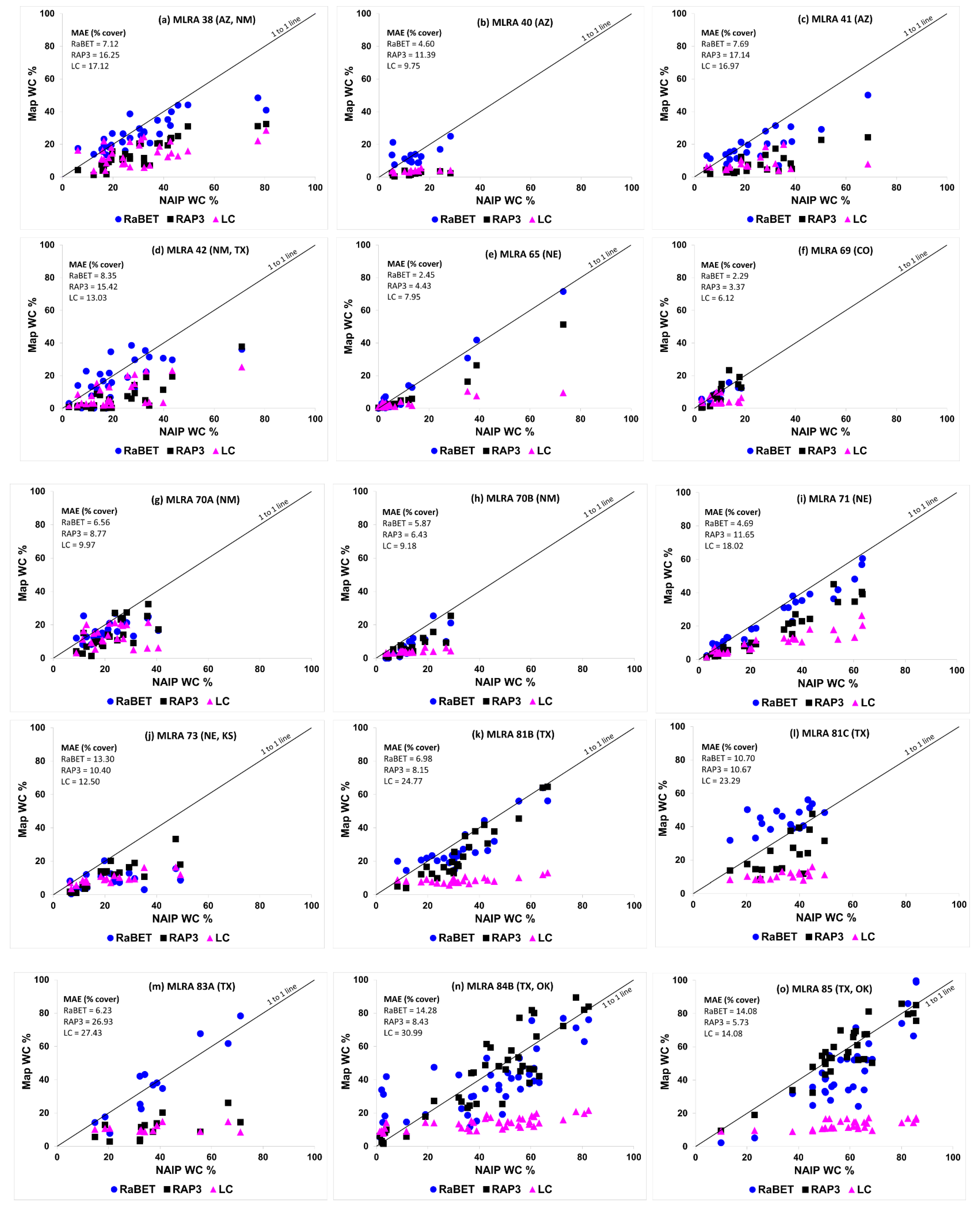
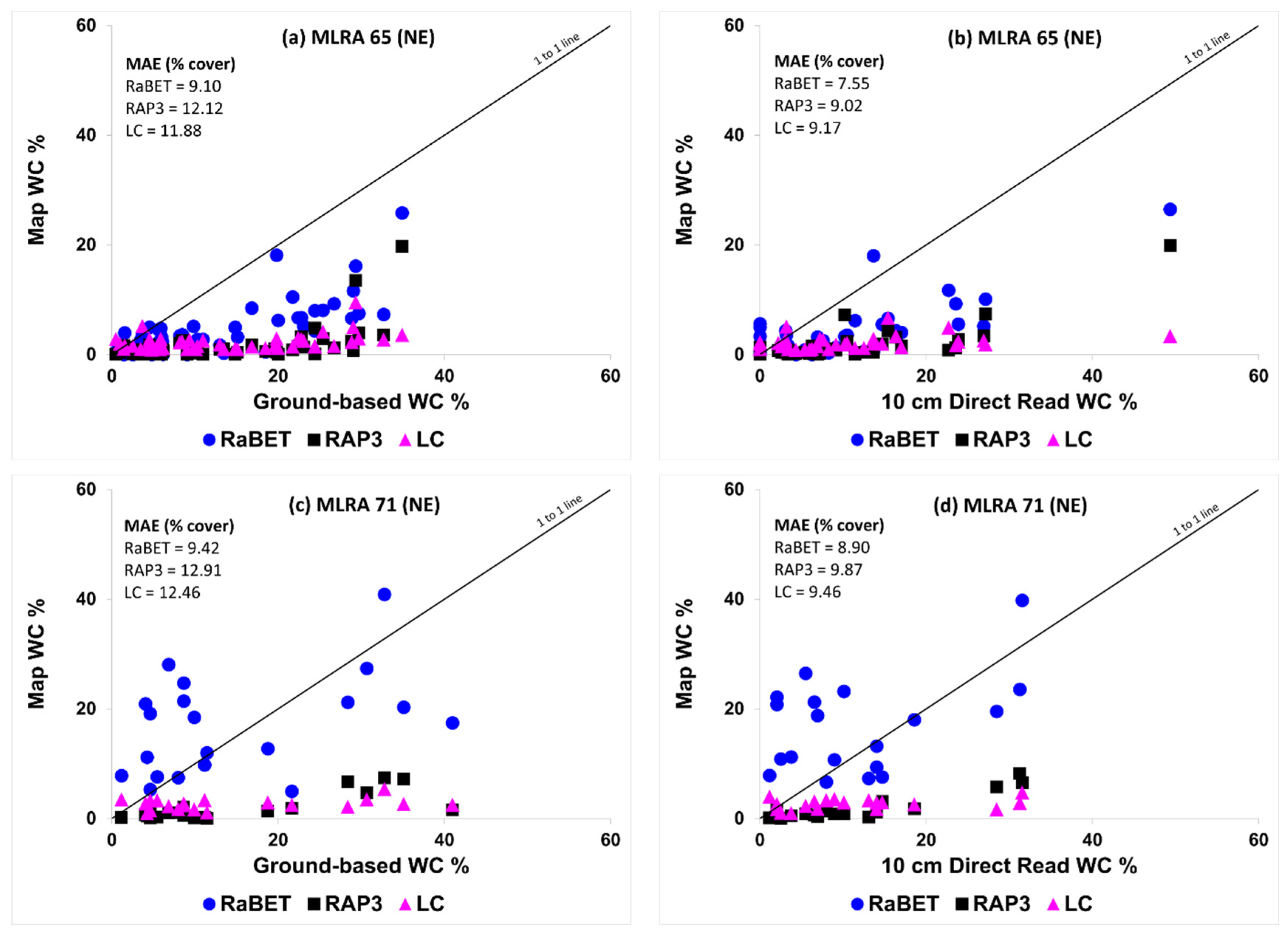
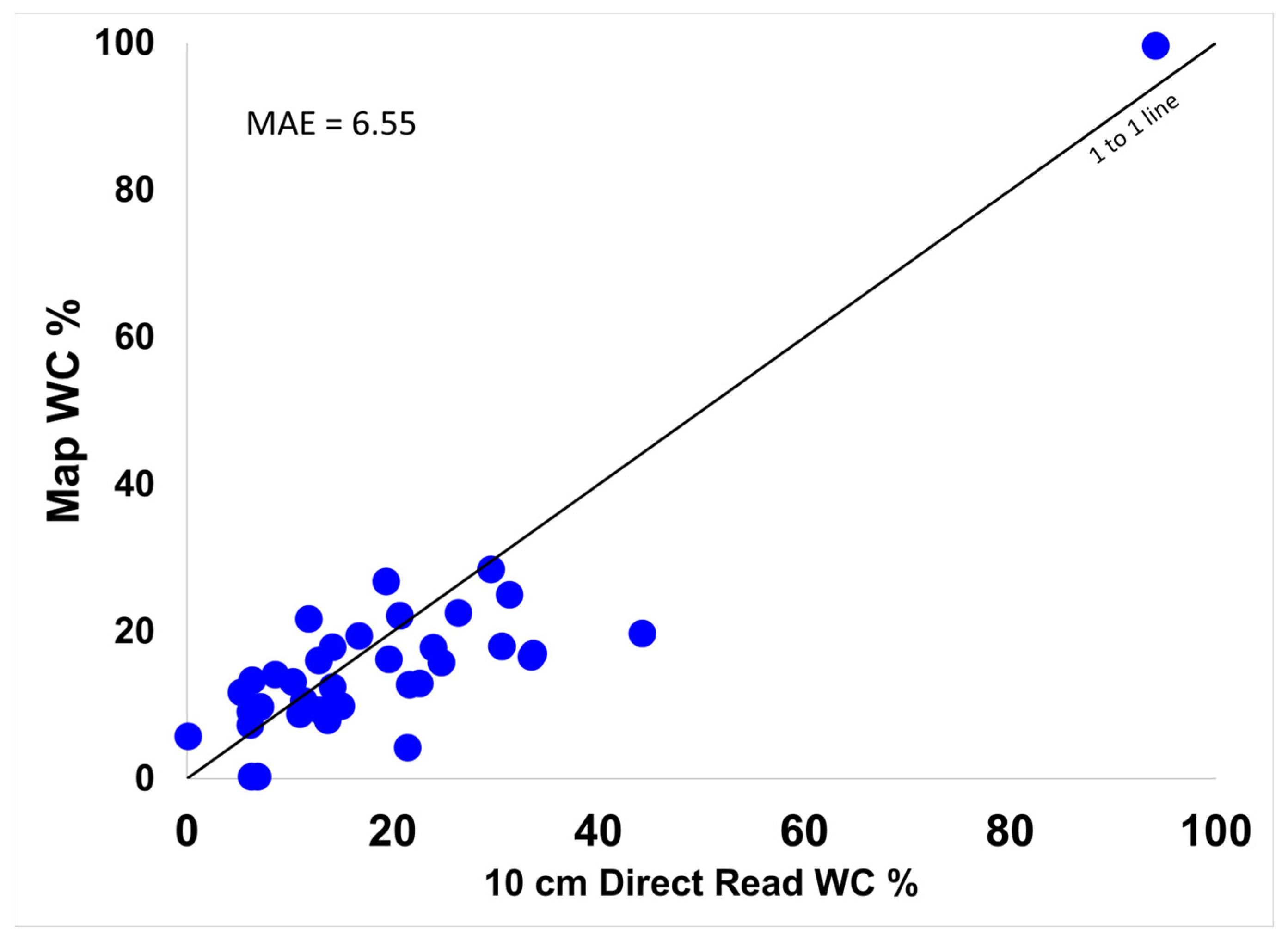
3.2. RaBET Validation and Comparison to RAP and LandCART

RaBET maps were validated at pasture-sized sample locations by comparing RaBET, NAIP, and 10 cm average woody cover values. NAIP samples used to develop multiple linear regression coefficients were excluded from the calculation of validation results. RaBET maps were compared with RAP and LandCART at NAIP and 10 cm sample locations for years shown in Table 2.

Map validation and comparison results are summarized in Figure 8. RaBET MAE varied by MLRA and ranged between 2.29% and 14.26%, with especially large errors in MLRAs 73, 84B, and 85, where RAP MAE was smaller than RaBET. The remaining 12 MLRA MAEs were smaller for RaBET than for RAP and LandCART. RAP had smaller MAEs than LandCART for all MLRAs.

Transect Line Comparisons for MLRA 65 and MLRA 71

In efforts to validate results, satellite-based maps are often compared to ground-based transects. MLRA 65 and MLRA 71 had large field campaigns of transect data collection, and comparisons of those data were made with RaBET, RAP, and LandCART maps from 2018 in MLRA 65 and 2021 in MLRA 71 (Figure 9a,c). RaBET had smaller MAE than RAP or LandCART; however, no map showed good relationships with ground-based woody cover.

Traditional field campaigns like those described are costly and time-consuming. Therefore, the use of fine-resolution (10 cm) aerial imagery as a substitute was explored. Transect lines from the ground-based sampling design were read directly from the imagery collected in 2020 for MLRA 65 and 2022 for MLRA 71. Directly read woody cover was compared with RaBET, RAP, and LandCART maps from 2018 in MLRA 65 and 2021 in MLRA 71 (Figure 9b,d). The relationships between directly read woody cover vs. map woody cover were better than ground-based vs. map woody cover. Out of the three maps, RaBET had the smallest MAE. No ground-based sampling data were available for MLRA 41, but a comparison of directly read and RaBET map data showed an MAE of 6.55 (Figure 10). Directly read woody cover was also compared to ground-based woody cover and correlations of 81% and 84% were found for MLRA 65 and MLRA 71, respectively.

4. Discussion

4.1. Motivation for the Project

Encroachment of woody species into perennial grasslands is a critical threat to grassland conservation in rangeland ecosystems. The expansion of these species into areas where they were previously minor components is well documented [4,39,40,41,42]; however, planning conservation treatments, monitoring outcomes, and conducting accurate assessments pose significant challenges, particularly when dealing with vast expanses of land while having limited resources [9,10,11,43].

In many cases, to meet program or planning deadlines, the field inventory does not take place; the planner estimates the amount and the extent of brush to treat and assigns a payment rate based on a non-defensible ocular estimate. This results in a lack of documentation of the true extent/degree of the concern, potentially inflated payment rates offered to the producer, unrealistic treatment objectives, and inadequate operation/maintenance plans to provide for long-term success.

Conservationists and land managers need an inexpensive, effective means of monitoring and documenting the effects of brush management conservation methods for decreasing degradation in rangeland systems. The key may be remote sensing-based geospatial tools that estimate woody canopy cover over time and produce rapid, accurate, cost-effective, reproducible assessments over vast and inaccessible areas [44,45,46]. RaBET was specifically developed to meet these needs.

4.2. Comparison of RaBET, RAP, and LandCART Map Products

RaBET, RAP, and LandCART map comparisons with classified pasture-sized NAIP imagery samples showed RaBET generally performed better than RAP and LandCART, with smaller MAE values (Figure 8). Studies have indicated that when working with smaller numbers of training samples, multiple linear regression performed better than advanced machine learning methods, while machine learning was preferred when large numbers of samples were available [47,48,49]. Our comparisons demonstrated that more novel machine learning methods will not always produce superior results. Figure 8 shows that regression with smaller numbers of training samples resulted in more accurate woody cover estimates for 80% of the MLRAs. The differences may be more strongly related to training sample size rather than number. RaBET used pasture-sized input, while samples for RAP and LandCART were essentially point data. The areas sampled for RaBET ranged from approximately 16 ha to 81 ha, whereas training sample areas used by RAP and LandCART (0.25 ha) were much smaller than a typical pasture. Such small sample sizes, even in large numbers, do not represent the landscape heterogeneity crucial for planning purposes.

RaBET addresses MLRA-specific landscapes and woody cover by employing phenology windows to enhance target/background contrast. Appropriate seasonal remote sensing data can reduce the influence of grass background greenness [50,51]. Where RaBET had especially large MAEs (MLRAs 73, 84B, 85), it is likely that multiple woody species were captured within the selected phenological window (Figure 8). In the future, this may be corrected using different windows and multiple ecoregion subdivisions for regression development. RaBET MAE was less than RAP and LandCART in the southwestern MLRAs (41, 42, 38, 40), which are characterized by multiple small-leaved woody species that are hard to distinguish, even in NAIP imagery. This may be due to the larger pasture-sized samples used by RaBET, which result in a better chance of capturing landscape variability.

4.3. Comparison of Map Validation Methods

When using remotely sensed data, the subject of “ground truthing” is often a consideration. It is common practice to collect ground-based transect data to compare with remote sensing-based vegetation cover estimates, and numerous studies have found approximate equivalence between plant canopy cover measured on the ground and that measured in image data [44,52,53,54]. In contrast, some studies showed the image-assessed canopy to be substantially different from the ground-assessed canopy [55,56]. The results from common field canopy measurement methods, including line or line-point intercept, cannot be assumed as “ground truth” due to a variety of biases that can be present [55]. In addition, this methodology relies solely on localized data acquired at specific moments of time and rarely adequately represents the spatial or spectral characteristics of the landscape.

The collection of traditional ground-based transect data is expensive and difficult to obtain due to the need for people, time, access, and transportation. In addition, these surveys can be inconsistent in covering areas the size of MLRAs [57,58]. As shown in Figure 9, all three tool maps had poor agreement with ground-based data. This may be the result of several factors. The field campaigns were carried out using large numbers of people (24 for MLRA 65 and 19 for MLRA 71) with varied experience and training. Having multiple people involved in data collection increases the potential for inter-observer bias as measurements are read and recorded. Topography and land ownership were also factors. Land access played a large role in where samples could be collected and topographic relief often caused alterations to transect layout and line lengths as read, particularly in MLRA 65. Preliminary training sessions were provided before collection in MLRA 71, and most collectors were employed by NRCS. This may have decreased some of the possible bias seen in MLRA 65 and resulted in slightly better results (Figure 9a,c).

Fine resolution imagery-based transect data can provide substantial benefits over traditionally collected field data. MLRA-wide imagery can be acquired over extensive areas in a single day (Figure 3), whereas it takes months to obtain similar coverage using ground-based methods (Figure 5). In the example of MLRA 41, with a team of four to six people reading ground transects and one person processing the data, collecting and processing data for one site takes approximately three hours plus travel time. This means that only two to three sites can be read in an eight-hour day, depending on travel time. Therefore, a maximum of fifteen sites can be completed during a five-day work week. In contrast, three people directly reading transect data from fine resolution (10 cm) imagery and one person processing the data requires approximately one hour per site. Thus, 24 sites could be read in an eight-hour day, leading to 120 sites being completed in the same five-day work week. This methodology was employed for MLRA 41 [59] and found to have satisfactory results with an MAE of 6.55 when 10 cm directly read woody cover was compared to map woody cover (Figure 10). These results, combined with correlations found between ground-based and 10 cm image-based woody cover (81% and 84% for MLRAs 65 and 71, respectively), show the promise of fine resolution imagery to bypass the limitations of traditional ground-based methods.

4.4. Contributions to Land Management

This work was developed to fulfill a need for the USDA-NRCS Conservation Effects Assessment Project (CEAP) [60], which is a multi-agency response to a request from Congress to provide accountability for public dollars spent. That request sought better transparency in reporting and documenting conservation practice effects that the public could understand and support.

Advances in sensor and camera technology and data distribution have made it possible to detect lower levels of vegetation cover at accuracies higher than previously possible [61]. By using high-resolution imagery paired with Landsat satellite imagery, and adapting regression relationships to landscapes present within specific MLRAs, RaBET provides accurate maps of the complete range of woody vegetation cover values (0–90+%) that allow for proactive, rather than only reactive, responses to woody encroachment. In addition, RaBET can be used to document and track woody cover levels before treatment and for many years after treatment, or simply track natural changes over time. Outputs of ready-made graphics and tabular statistics from the change analysis can be added directly into required documentation, streamlining the reporting process.

4.5. Applying Remote Sensing for Woody Vegetation Mapping

When attempting to solve a problem using remotely sensed data, there are several important factors that must be considered: the scale of the problem (time and space); the final product to be delivered (an application versus a manuscript); the characteristics of the study area; available resources (data, computing, budgetary, personnel, expertise). These factors will dictate the best method to solve the problem.

For this work, a method was needed that could be adapted to various MLRA landscapes. Regression offered the flexibility to be tailored to the wide range in climate, soils, and topography that result in diverse rangeland landscapes. Using 4-year Landsat vegetation index composites helped to fill in data gaps and smoothed precipitation influences that can occur with within a single year and across landscapes [62]. However, the trade-off in using 4-year composites is that identifying dates of vegetation change (e.g., brush removal, fire) can become more difficult.

Focusing only on woody vegetation canopy cover allowed us to utilize a streamlined approach. No ancillary datasets were required (e.g., precipitation, soils, elevation); maps of existing vegetation were not needed; and very basic supervised classification (woody vs. non-woody) could be used.

We believe this method could be used with other satellite image data (e.g., Sentinel-2 https://sentinel.esa.int/web/sentinel/home, accessed on 13 October 2023 or Harmonized Landsat and Sentinel-2 https://hls.gsfc.nasa.gov, accessed on 13 October 2023), with a source of high-resolution color-infrared imagery for training samples and validation data. In this work, NAIP imagery was used due to its no-cost, wall-to-wall coverage of the United States. Acquisition times were sometimes suboptimal, leading to increased challenges for personnel classifying training samples, but the NAIP data were satisfactory for our purposes. Other sources of high-resolution imagery could also be used with this method. On the commercial side, Planet SkySat imagery (https://planet.com, accessed on 13 October 2023) is 0.5 m resolution and can be tasked for acquisitions globally. Privately contracted aerial flights are another resource and provide the ability to specify acquisition timing and spatial resolution. Finally, when possible, it is ideal to have local expert knowledge of project landscapes for guidance in high-resolution image interpretation and product validation.

5. Conclusions

Over 160 million hectares of rangelands in the central and western United States depend on effective management of woody species, including eradication, to preserve and improve clean water, reduce disaster risk, support productive and stable soils, continuous food supply, and many other goods and services. Until now, there has been no consistent, effective means for land managers to document and assess the success of their efforts to manage woody species. We developed RaBET to answer this need. Using transparent, repeatable methods, RaBET delivers woody canopy cover maps at field scales suited for conservation planning by land managers on rangelands.

This work found that when compared to more novel machine learning methods, a simpler multiple linear regression method worked better for quantifying woody canopy cover on heterogenous landscapes. When compared to traditional ground-based methods of acquiring map validation data, reading woody cover measurements directly from fine-resolution imagery showed promise for decreasing the amount of time and resources needed to collect these data.

Future research will explore the use of data fusion methods to identify and create species-specific maps of woody species encroaching on rangeland.

References

1. Archer, S.R.; Andersen, E.M.; Predick, K.I.; Schwinning, S.; Steidl, R.J.; Woods, S.R.; Briske, D.D. Woody plant encroachment: Causes and consequences. In Rangeland Systems: Processes, Management and Challenges; Springer International Publishing: Cham, Switzerland, 2017; pp. 25–84. [Google Scholar]
2. Ding, J.; Eldridge, D. The success of woody plant removal depends on encroachment stage and plant traits. Nat. Plants 2023, 9, 58–67. [Google Scholar] [CrossRef] [PubMed]
3. Eldridge, D.J.; Bowker, M.A.; Maestre, F.T.; Roger, E.; Reynolds, J.F.; Whitford, W.G. Impacts of shrub encroachment on ecosystem structure and functioning: Towards a global synthesis. Ecol. Lett. 2011, 14, 709–722. [Google Scholar] [CrossRef] [PubMed]
4. Archer, S.; Boutton, T.W.; Hibbard, K.A. Trees in grasslands: Biogeochemical consequences of woody plant expansion. In Global Biogeochemical Cycles in the Climate System; Schulz, M., Heimann, S., Harrison, E., Holland, J., Lloyd, I., Eds.; Academic Press: San Diego, CA, USA, 2001; pp. 115–138. [Google Scholar]
5. Londe, D.; Cady, S.; Elmore, R.D.; Fuhlendorf, S. Woody plant encroachment pervasive across three socially and ecologically diverse ecoregions. Ecol. Soc. 2022, 27, 11. [Google Scholar] [CrossRef]
6. Scifres, C.J. Brush Management: Principles and Practices for Texas and the Southwest; Texas A&M University Press: College Station, TX, USA, 1980. [Google Scholar]
7. Hamilton, W.T.; McGinty, A.; Ueckert, D.N.; Hanselka, C.W.; Lee, M.R. Brush Managment: Past, Present, Future; Texas A&M University Press: College Station, TX, USA, 2004. [Google Scholar]
8. Welch, T.G. Brush Management Methods; Texas A&M Agrilife Extension: College Station, TX, USA, 2000. [Google Scholar]
9. Scholtz, R.; Fuhlendorf, S.D.; Uden, D.R.; Allred, B.W.; Jones, M.O.; Naugle, D.E.; Twidwell, D. Challenges of brush management treatment effectiveness in southern Great Plains, United States. Rangel. Ecol. Manag. 2021, 77, 57–65. [Google Scholar] [CrossRef]
10. Jansen, V.S.; Kolden, C.A.; Schmalz, H.J. The development of near real-time biomass and cover estimates for adaptive rangeland management using Landsat 7 and Landsat 8 surface reflectance products. Remote Sens. 2018, 10, 1057. [Google Scholar] [CrossRef]
11. Mansour, K.; Mutanga, O.; Everson, T. Remote sensing based indicators of vegetation species for assessing rangeland degradation: Opportunities and challenges. Afr. J. Agric. Res. 2012, 7, 3261–3270. [Google Scholar] [CrossRef]
12. Robinson, N.P.; Allred, B.W.; Naugle, D.E.; Jones, M.O. Patterns of rangeland productivity and land ownership: Implications for conservation and management. Ecol. Appl. 2019, 29, e01862. [Google Scholar] [CrossRef]
13. Stubbs, M. Environmental Quality Incentives Program (EQIP): Status and Issues; Congressional Research Service: Washington, DC, USA, 2010.
14. Briske, D.D.; Jolley, L.W.; Duriancik, L.F.; Dobrowolski, J.P. Introduction to the conservation effects assessment project and the rangeland literature synthesis. In Conservation Benefits of Rangeland Practices: Assessment, Recommendations, and Knowledge Gaps; Natural Resources Conservation Service: Washington, DC, USA, 2011; pp. 4–8. [Google Scholar]
15. Rigge, M.; Shi, H.; Homer, C.; Danielson, P.; Granneman, B. Long-term trajectories of fractional component change in the Northern Great Basin, USA. Ecosphere 2019, 10, e02762. [Google Scholar] [CrossRef]
16. Boyte, S.P.; Wylie, B.K.; Major, D.J. Cheatgrass percent cover change: Comparing recent estimates to climate change-driven predictions in the northern Great Basin. Rangel. Ecol. Manag. 2016, 69, 265–279. [Google Scholar] [CrossRef]
17. Henderson, E.B.; Bell, D.M.; Gregory, M.J. Vegetation mapping to support greater sage-grouse habitat monitoring and management: Multi-or univariate approach? Ecosphere 2019, 10, e02838. [Google Scholar] [CrossRef]
18. Falkowski, M.J.; Evans, J.S.; Naugle, D.E.; Hagen, C.A.; Carleton, S.A.; Maestas, J.D.; Henareh Khalyani, A.; Poznanovic, A.J.; Lawrence, A.J. Mapping tree canopy cover in support of proactive prairie grouse conservation in western North America. Rangel. Ecol. Manag. 2017, 70, 15–24. [Google Scholar] [CrossRef]
19. Allred, B.W.; Bestelmeyer, B.T.; Boyd, C.S.; Brown, C.; Davies, K.W.; Duniway, M.C.; Ellsworth, L.M.; Erickson, T.A.; Fuhlendorf, S.D.; Griffiths, T.V.; et al. Improving Landsat predictions of rangeland fractional cover with multitask learning and uncertainty. Methods Ecol. Evol. 2021, 12, 841–849. [Google Scholar] [CrossRef]
20. Okin, G.; Zhou, B.; Duniway, M.; Cole, C.; Savage, S.; Litschert, S.; Liddle, J. Landscape Cover Analysis and Reporting Tools V1.0. Available online: https://landcart-301816.wm.r.appspot.com/#/ (accessed on 1 April 2023).
21. United States Department of Agriculture, Natural Resources Conservation Service. Land Resource Regions and Major Land Resource Areas of the United States, the Caribbean, and the Pacific Basin; U.S. Department of Agriculture Handbook 296: Washington, DC, USA, 2006.
22. Mountrakis, G.; Im, J.; Ogole, C. Support vector machines in remote sensing: A review. ISPRS J. Photogramm. Remote Sens. 2011, 66, 247–259. [Google Scholar] [CrossRef]
23. Stehman, S. Estimating the kappa coefficient and its variance under stratified random sampling. Photogramm. Eng. Remote Sens. 1996, 62, 401–407. [Google Scholar]
24. Karasiak, N.; Fauvel, M.; Dejoux, J.-F.; Monteil, C.; Sheeren, D. Optimal dates for deciduous tree species mapping using full years Sentinel-2 time series in south west France. ISPRS Ann. Photogramm. Remote Sens. Spat. Inf. Sci. 2020, V-3-2020, 469–476. [Google Scholar] [CrossRef]
25. Van Leeuwen, W.J.D.; Davison, J.E.; Casady, G.M.; Marsh, S.E. Phenological characterization of Desert Sky Island vegetation communities with remotely sensed and climate time series data. Remote Sens. 2010, 2, 388–415. [Google Scholar] [CrossRef]
26. Casady, G.M.; van Leeuwen, W.J.D.; Reed, B.C. Estimating winter annual biomass in the Sonoran and Mojave deserts with satellite- and ground-based observations. Remote Sens. 2013, 5, 909–926. [Google Scholar] [CrossRef]
27. Smith, W.K.; Dannenberg, M.P.; Yan, D.; Herrmann, S.; Barnes, M.L.; Barron-Gafford, G.A.; Biederman, J.A.; Ferrenberg, S.; Fox, A.M.; Hudson, A.; et al. Remote sensing of dryland ecosystem structure and function: Progress, challenges, and opportunities. Remote Sens. Environ. 2019, 233, 111401. [Google Scholar] [CrossRef]
28. Gitelson, A.A.; Kaufman, Y.J.; Merzlyak, M.N. Use of green channel in remote sensing of global vegetation from EOS-MODIS. Remote Sens. Environ. 1996, 58, 289–298. [Google Scholar] [CrossRef]
29. Marsett, R.C.; Qi, J.; Heilman, P.; Biedenbender, S.H.; Watson, M.C.; Amer, S.; Weltz, M.; Goodrich, D.; Marsett, R. Remote sensing for grassland management in the arid southwest. Rangel. Ecol. Manag. 2006, 59, 530–540. [Google Scholar] [CrossRef]
30. Waller, E.K.; Villarreal, M.L.; Poitras, T.B.; Nauman, T.W.; Duniway, M.C. Landsat time series analysis of fractional plant cover changes on abandoned energy development sites. Int. J. Appl. Earth Obs. Geoinf. 2018, 73, 407–419. [Google Scholar] [CrossRef]
31. Qi, J.; Chehbouni, A.; Huete, A.R.; Kerr, Y.H.; Sorooshian, S. A modified soil adjusted vegetation index. Remote Sens. Environ. 1994, 48, 119–126. [Google Scholar] [CrossRef]
32. Liu, Z.; Huang, J.; Wu, X.; Dong, Y. Comparison of vegetation indices and red-edge parameters for estimating grassland cover from canopy reflectance data. J. Integr. Plant Biol. 2007, 49, 299–306. [Google Scholar] [CrossRef]
33. McNairn, H.; Protz, R. Mapping corn residue cover on agricultural fields in Oxford County, Ontario, using thematic mapper. Can. J. Remote 1993, 19, 152–159. [Google Scholar] [CrossRef]
34. Dingaan, M.N.V.; Tsubo, M. Improved assessment of pasture availability in semi-arid grassland of South Africa. Environ. Monit. Assess. 2019, 191, 733. [Google Scholar] [CrossRef]
35. Zhang, J.; Okin, G.S.; Zhou, B. Assimilating optical satellite remote sensing images and field data to predict surface indicators in the Western US: Assessing error in satellite predictions based on large geographical datasets with the use of machine learning. Remote Sens. Environ. 2019, 233, 111382. [Google Scholar] [CrossRef]
36. Zhou, B.; Okin, G.S.; Zhang, J. Leverageing Google Earth Engine (GEE) and machine learning algorithms to incorporate in situ measurement from different times for rangelands monitoring. Remote Sens. Environ. 2020, 236, 111521. [Google Scholar] [CrossRef]
37. Herrick, J.E. Monitoring Manual for Grassland, Shrubland and Savanna Ecosystems, Volume 1: Quick Start; USDA-ARS Jornada Experimental Range; The University of Arizona Press: Tucson, AZ, USA, 2005. [Google Scholar]
38. Holifield Collins, C.D.; Kautz, M.A.; Tiller, R.; Lohani, S.; Ponce-Campos, G.; Hottenstein, J.; Metz, L.J. Development of an integrated multiplatform approach for assessing brush management conservation efforts in semiarid rangelands. J. Appl. Remote Sens. 2015, 9, 096057. [Google Scholar] [CrossRef]
39. Steinauer, E.M.; Bragg, T.B. Ponderosa pine (Pinus ponderosa) invasion of Nebraska Sandhills prairie. Am. Midl. Nat. 1987, 118, 358–365. [Google Scholar] [CrossRef]
40. Eggemeyer, K.D.; Awada, T.; Wedin, D.A.; Harvey, F.E.; Zhou, X. Ecophysiology of two native invasive woody species and two dominant warm-season grasses in the semiarid grasslands of the Nebraska Sandhills. Int. J. Plant Sci. 2006, 167, 991–999. [Google Scholar] [CrossRef]
41. Barger, N.N.; Archer, S.R.; Campbell, J.L.; Huang, C.Y.; Morton, J.A.; Knapp, A.K. Woody plant proliferation in North American drylands: A synthesis of impacts on ecosystem carbon balance. J. Geophys. Res. Biogeosci. 2011, 116, G4. [Google Scholar] [CrossRef]
42. Walker, T.L., Jr.; Hoback, W.W. Effects of invasive eastern redcedar on capture rates of Nicrophorus americanus and other Silphidae. Environ. Entomol. 2007, 36, 297–307. [Google Scholar] [CrossRef] [PubMed]
43. Ucar, Z.; Bettinger, P.; Merry, K.; Akbulut, R.; Siry, J. Estimation of urban woody vegetation cover using multispectral imagery and LiDAR. Urban For. Urban Green. 2018, 29, 248–260. [Google Scholar] [CrossRef]
44. Boswell, A.; Petersen, S.; Roundy, B.; Jensen, R.; Summers, D.; Hulet, A. Rangeland monitoring using remote sensing: Comparison of cover estimates from field measurements and image analysis. AIMS Environ. Sci. 2017, 4, 1–16. [Google Scholar] [CrossRef]
45. Whiteside, T.G.; Esparon, A.J.; Bartolo, R.E. A semi-automated approach for quantitative mapping of woody cover from historical time series aerial photography and satellite imagery. Ecol. Inform. 2020, 55, 101012. [Google Scholar] [CrossRef]
46. Fern, R.R.; Foxley, E.A.; Bruno, A.; Morrison, M.L. Suitability of NDVI and OSAVI as estimators of green biomass and coverage in a semi-arid rangeland. Ecol. Indic. 2018, 94, 16–21. [Google Scholar] [CrossRef]
47. Lo, A.; Diouf, A.A.; Diedhiou, I.; Basséne, C.D.E.; Leroux, L.; Tagesson, T.; Fensholt, R.; Hiernaux, P.; Mottet, A.; Taugourdeau, S.; et al. Dry season forage assessment across senegalese rangelands using earth observation data. Front. Environ. Sci. 2022, 10, 931299. [Google Scholar] [CrossRef]
48. Ding, Y.; Zhang, H.; Wang, Z.; Xie, Q.; Wang, Y.; Liu, L.; Hall, C. A comparison of estimating crop residue cover from Sentinel-2 data using empirical regressions and machine learning methods. Remote Sens. 2020, 12, 1470. [Google Scholar] [CrossRef]
49. Wang, L.; Zhou, X.; Zhu, X.; Dong, Z.; Guo, W. Estimation of biomass in wheat using random forest regression algorithm and remote sensing data. Crop J. 2016, 4, 212–219. [Google Scholar] [CrossRef]
50. Cao, X.; Liu, Y.; Cui, X.; Chen, J.; Chen, X. Mechanisms, monitoring and modeling of shrub encroachment into grassland: A review. Int. J. Digit. Earth 2019, 12, 625–641. [Google Scholar] [CrossRef]
51. Selkowitz, D.J. A comparison of multi-spectral, multi-angular, and multi-temporal remote sensing datasets for fractional shrub canopy mapping in arctic Alaska. Remote Sens. Environ. 2010, 114, 1338–1352. [Google Scholar] [CrossRef]
52. Booth, D.T.; Cox, S.E.; Meikle, T.; Zuuring, H.R. Ground-cover measurements: Assessing correlation among aerial and ground-based methods. Environ. Manag. 2008, 42, 1091–1100. [Google Scholar] [CrossRef] [PubMed]
53. Boswell, A.K. Rangeland Monitoring Using Remote Sensing: An Assessment of Vegetation Cover Comparing Field-Based Sampling and Image Analysis Techniques. Master’s Thesis, Brigham Young University, Provo, UT, USA, 2015. [Google Scholar]
54. Karl, J.W.; Herrick, J.E.; Pyke, D.A. Monitoring protocols: Options, approaches, implementation, benefits. In Rangeland Systems: Processes, Management and Challenges; Springer: Berlin/Heidelberg, Germany, 2017; pp. 527–567. [Google Scholar]
55. Booth, D.T.; Cox, S.E.; Meikle, T.W.; Fitzgerald, C. The accuracy of ground-cover measurements. Rangel. Ecol. Manag. 2006, 59, 179–188. [Google Scholar] [CrossRef]
56. Cagney, J.; Cox, S.E.; Booth, D.T. Comparison of point intercept and image analysis for monitoring rangeland transects. Rangel. Ecol. Manag. 2011, 64, 309–315. [Google Scholar] [CrossRef]
57. Ramoelo, A.; Stolter, C.; Joubert, D.; Cho, M.A.; Groengroeft, A.; Madibela, O.R.; Zimmermann, I.; Pringle, H. Rangeland monitoring and assessment: A review. Biodivers. Ecol. 2018, 6, 170–176. [Google Scholar] [CrossRef]
58. Soubry, I.; Guo, X. Quantifying woody plant encroachment in grasslands: A review on remote sensing approaches. Can. J. Remote 2022, 48, 337–378. [Google Scholar] [CrossRef]
59. Holifield Collins, C.; Skirvin, S.; Curley, D.; Corrales, A.; Winston, Z.; Heilman, P.; Metz, L. Hopping onto airborne-based validation for Landsat-based Rangeland Brush Estimation Tool (RaBET) woody cover maps. In Proceedings of the American Geophysical Union, Chicago, IL, USA, 12–16 December 2022. [Google Scholar]
60. Briske, D.D. (Ed.) Conservation Benefits of Rangeland Practices: Assessment, Recommendations, and Knowledge Gaps; United States Department of Agriculture, Natural Resources Conservation Service: Washington, DC, USA, 2011; p. 429.
61. Leprieur, C.; Kerr, Y.H.; Mastorchio, S.; Meunier, J.C. Monitoring vegetation cover across semi-arid regions: Comparison of remote observations from various scales. Int. J. Remote Sens. 2000, 21, 281–300. [Google Scholar] [CrossRef]
62. Anchang, J.Y.; Prihodko, L.; Ji, W.; Kumar, S.S.; Ross, C.W.; Yu, Q.; Lind, B.; Sarr, M.A.; Diouf, A.A.; Hanan, N.P. Toward operational mapping of woody canopy cover in tropical savannas using Google Earth Engine. Front. Environ. Sci. 2020, 8, 4. [Google Scholar] [CrossRef]
Figure 1. Map showing the coverage of MLRAs used in the study [21] and locations of National Agriculture Imagery Program (NAIP) pasture-sized image samples.
Remotesensing 15 05102 g001
Figure 2. Overview of relationships of project data and methods. Uncolored boxes are dataset inputs. Orange boxes are calculated operations. Blue boxes are project results. Green boxes are new and existing map products.
Remotesensing 15 05102 g002
Figure 3. Maps showing pasture-sized 10 cm imagery sites within (A) MLRA 41 and (B) MLRAs 65 and 71.
Remotesensing 15 05102 g003
Figure 4. Maps showing pasture-sized examples of: (a) NAIP imagery and Landsat vegetation indices; (b) Woody Vegetation Index (WVI); (c) Modified Soil Adjusted Index (MSAVI2); and (d) Normalized Difference Index 5 (NDI5).
Remotesensing 15 05102 g004
Figure 5. Map showing locations of 77 ground transect sampling sites within MLRAs 65 and 71.
Remotesensing 15 05102 g005
Figure 6. Example of process for aggregating 1 m resolution imagery to 30 m resolution: (a) a section of input image; (b) a section of input image classified as woody or non-woody; (c) sample of aggregation calculation of percent woody cover for a 5 × 5 m output pixel; (d) example of classified NAIP aggregated to 30 m resolution [38].
Remotesensing 15 05102 g006
Figure 7. Workflow for generation of RaBET woody canopy cover maps.
Remotesensing 15 05102 g007
Figure 8. Validation and comparisons for RaBET, RAP, and LandCART (LC) woody cover maps for all MLRAs. Reference NAIP sample average woody cover is plotted against average map woody cover by sample with the 1:1 line reference line shown: samples falling closer to the 1:1 line indicate more accurate map results. Average sample mean absolute error (MAE) is summarized for all 3 maps in the upper left corner of each MLRA panel: (a) 38; (b) 40; (c) 41; (d) 42; (e) 65; (f) 69; (g) 70A; (h) 70B; (i) 71; (j) 73; (k) 81B; (l) 81C; (m) 83A; (n) 84B; (o) 85.
Remotesensing 15 05102 g008
Figure 9. Comparison of site average map woody cover for ground-based transect sites and 10 cm directly read sites. Ground-based site average woody cover is plotted against average map woody cover by site with the 1:1 reference line shown: (a) MLRA 65 and (c) MLRA 71. Directly read site average woody cover is plotted against average map woody cover by site with the 1:1 reference line shown: (b) MLRA 65 and (d) MLRA 71. Samples falling closer to the 1:1 line indicate more accurate map results. Average sample mean absolute error (MAE) is summarized for all 3 maps in the upper left corner of each panel.
Remotesensing 15 05102 g009
Figure 10. Comparison of site average 2021 RaBET map woody cover and 10 cm directly read sites in MLRA 41 in Arizona (AZ). Directly read site average woody cover is plotted against average map woody cover by site with the 1:1 reference line shown. Average site mean absolute error percent (MAE) is displayed in the upper left corner of the panel.
Remotesensing 15 05102 g010