Examining the Potential of Sentinel Imagery and Ensemble Algorithms for Estimating Aboveground Biomass in a Tropical Dry Forest

Abstract

Accurate estimations of aboveground biomass (AGB) in tropical forests are crucial for maintaining carbon stocks and ensuring effective forest management. By combining remote sensing (RS) data with ensemble algorithms, reliable AGB estimates in forests can be obtained. In this context, the freely available Sentinel-1 (S-1 SAR) and Sentinel 2 multispectral imagery (S-2 MSI) data have a significant role in enhancing accurate AGB estimations at a lower cost, which is relevant for the tropical dry forest (TDF) regions where AGB estimation is uncertain or there is a lack of comprehensive exploration. This study aims to address this gap by presenting a cost-effective and reliable AGB estimation approach in the TDF region of Colombia. For this purpose, we modeled and compared the performance of two ensemble algorithms, random forest (RF) and extreme gradient boosting (XGBoost), to estimate AGB using three predictor categories (polarizations/textures, spectral bands/vegetation indices, and a combination of both). We then examined the modeling potential of S-1 SAR and S-2 MSI imagery in predicting forest AGB and subsequently identified the most suitable variables. To construct AGB models’ field data, we employed a clustered distributed sampling approach involving 100 subsample plots, each with an area of 400 m². Stepwise multiple linear regression was applied to identify suitable predictors from the original satellite bands, vegetation indices, and texture metrics. To produce a map of AGB, predicted AGB values were calculated for every pixel within a specific satellite subscene using the most effective ensemble algorithm. Our study findings show that the RF model, which employed combined predictor sets, displayed superior performance when evaluated against the independent validation set. The RF model successfully estimated AGB with a high degree of accuracy, achieving an R² value of 0.78 and an RMSE value of 42.25 Mg/ha⁻¹. In contrast, the XGBoost model performed less accurately, obtaining an R² value of only 0.60 and an RMSE value of 48.41 Mg/ha⁻¹. The results also indicate that S-2 vegetation indices data were more appropriate for this purpose than S-1 texture data. Despite this, S-1 cross-polarized textures were necessary during the dry season for the combined datasets. The top predictive variables for S-2 images were cab and cw, as well as red-edge bands during the wet season. As for S-1 images, texture D_VH _Hom during the dry season was the most important variable for explaining performance. Overall, the proposed approach of using freely available Sentinel data seems to improve the accuracy of AGB estimation in heterogeneous forest cover and, as such, they should be recommended as a data source for forest AGB assessment.

1. Introduction

Tropical forests are the paramount source for about 25% of the global terrestrial carbon [1]. They also have the potential to mitigate climate change [2] if properly managed. An important step in this process is the assessment of carbon level sequestration by forests through consistent and accurate measurements of AGB [3,4]. Consistent measurements also provide the basis for reliable implementation of Reducing Emissions from Deforestation and Forest Degradation, plus the Sustainable Management of Forests (REDD+) and forest AGB maps [2,3]. Typically, forest AGB can be measured using field [5] or RS approaches [3]. However, field measurement of AGB is a destructive, impractical, and overly expensive approach for assessment of very large areas [6]. On the other hand, the RS approach of integrating field data (forest inventory plots) can be a cost-effective method for the estimation and mapping of forest AGB over large geographic scales [7]. However, the ability of RS to estimate AGB varies depending on the sensor used, with some sensors being more effective and more accurate than others [6,8,9,10,11].

Various approaches to estimating AGB using RS and field plot datasets based on single passive and active sensors have been widely used at different scales and in tropical forests [3,12,13]. Passive optical RS imagery (medium resolution, e.g., Landsat, Sentinel-2, ASTER), often associated with data-derived features such as spectral reflectance, vegetation indices, spatial texture, and forest canopy properties, have been shown to be closely related to forest AGB [12,14,15,16,17]. The main motivation for their use is their free availability for resource-constrained regions [3]. In addition, most medium-resolution imagery is characterized by a spatial resolution similar to the size of sample plots in national forest inventories, which reduces the error in matching pixels to the field plots and leads to improved estimation results [18]. However, its use is hampered by the problems of estimation accuracy and uncertainty due to the spectral saturation effect in complex vegetation such as tropical forests [16,18,19], limited penetration capacity through clouds, and poor information on the vertical distribution of forest structure [20].

In contrast to passive optical RS data, active sensors such as synthetic aperture radar (SAR) and light detection and ranging (LiDAR) have also been shown to have several advantages for estimating forest AGB [6,11,13,21,22]. Microwave-based SAR imagery is cloud independent and can determine the moisture content of vegetation [23]. Depending on the frequency used, SAR is able to penetrate the vegetation and intersect the main components of the AGB, i.e., the tree trunks and branches [24]. The intensity of the radar backscatter signal is then related to its physical structure or AGB. Thus, as the intensity of the radar backscatter increases, so does the AGB of the forest. In fact, the longer wavelengths (L- and P-band SAR) are more sensitive to forest AGB, which has made them suitable for AGB estimation studies [13,23,24,25]. However, mapping forest AGB using satellite SAR data does have some limitations. Their long-wavelength band data are expensive. And although they can penetrate vegetation, the short-wavelength (X- and C-band) SAR also has low penetration and saturation problems in tropical heterogeneous forests [26], where AGB levels generally exceed 200–250 Mg/ha⁻¹. On the other hand, light detection and ranging (LiDAR) can provide detailed measurements of vegetation structure, favoring accurate AGB estimates for diverse forests without saturation at higher AGB levels [21]. However, the LiDAR system is limited by its high cost per area, lack of spectral information, and unavailability of large datasets, making regional AGB estimation with airborne LiDAR unfeasible [27], especially in countries with tropical forests. To address this limitation, several studies focus on the complementary approaches of using different SAR and optical datasets, concluding that their combined use provides better results than the use of single sensors [6,11,12,28,29,30,31]. SARs are sensitive to roughness, texture, and moisture, whereas optical reflectance is sensitive to physiological conditions. These two spectral domains therefore provide complementary information.

The Sentinel mission has both medium-resolution SAR Sentinel-1 (S-1) and optical Sentinel-2 (S-2) multispectral imagery (MSI) data that are freely available worldwide. This provides an excellent opportunity to combine SAR and optical MSI datasets to improve the assessment of the accuracy of the tropical forest AGB and the mapping capability in heterogeneous vegetation areas. The S-2 MSI provides 13 multispectral bands, including three novel red-edge bands at 20 m spatial resolution, a component missing from previous multispectral sensors [32]. These bands are expected to contribute to improved AGB estimation and mapping [18]. In addition, S-2 MSI and its products (e.g., vegetation indices) can be compensated to some extent by the polarizations of the S-1 C-band SAR, which provides more information on vertical structure due to its ability to penetrate to a certain depth in the forest canopy [33], thus increasing the mapping capacity, especially where there is less foliage. Several studies have shown that the combination of Sentinel imagery can provide accurate estimates of various biophysical variables, including forest AGB. For example, Castillo et al. [34] estimated and mapped the AGB of Philippine mangrove forests using Sentinel imagery. Their method showed that the red-edge bands, which are more sensitive to vegetation, should provide new opportunities for AGB estimation. Chen et al. [35] investigated the combination of Sentinel imagery and reported that texture characteristics of S-1 and vegetation biophysical variables of S-2 were the best methods for mapping AGB. Furthermore, Laurin et al. [36] confirmed that the combination of S-1 with ALOS-2 and S-2 imagery for the estimation of AGB of broad leaf forests in central Italy improved the accuracy and reduced the saturation problem. Other studies have also confirmed the suitability of combining Sentinel imagery for AGB prediction models [37,38,39].

Combining RS and AGB plot information also presents a number of challenges. These include excessive metric dimensionality, information redundancy, and the selection of the optimal estimation model [11]. Parametric methods have traditionally been used to estimate AGB models, but they are unable to deal with the complicated non-linearity in complex tropical forests [3]. Non-parametric algorithms, such as SVM [40,41,42], ANN [35,43,44], K-NN [45,46,47], RF [39,48,49,50,51,52], and XGBoosting [53], have been shown to provide more accurate results, as they are less affected by forest factors, can handle high data dimensionality, and can effectively establish complicated non-linear relationships between AGB plot measurements and RS predictors [3,54]. Ghosh and Behera [52] evaluated the estimation effectiveness of RF and stochastic gradient boosting (SGB) models to estimate the AGB of two plantations in a dense tropical forest in India using S-1 and S-2 data and products (i.e., vegetation indices and SAR textures). The RF model gave better results than the SGB model for both plantation areas (RF; R² = 0.71; RMSE = 105 Mg/ha⁻¹ and R² = 0.58 vs. SGB; R² = 0.60; RMSE = 79.45 Mg/ha⁻¹ and R² = 0.57). Chen et al. [51] compared the performance of different algorithms, two parametric and three non-parametric methods SVR, ANN, and RF, for AGB RS estimation of broadleaved forest using Sentinel imagery and found that the RF algorithm performed the best (R² = 0.9; RMSE = 61.1 Mg/ha⁻¹). David et al. [39] also compared the AGB performance of RF with a linear parametric model in an African dryland forest using Sentinel data and found that RF had optimal performance (R² = 0.95; RMSE = 0.25 Mg/ha⁻¹). The performance of combining Sentinel images and using non-parametric ensemble algorithms in the TDF has so far been the subject of relatively few experiments [39]. There is therefore a need to assess the potential and effectiveness of the ensemble algorithms for AGB forest estimation, particularly using Sentinel data.

Despite TDFs’ global importance as a reservoir for about 18% of the global carbon stocks stored in all tropical forests [55] and high loss and conversion rates in Colombia [56], there is limited discussion in scientific literature regarding the development of effective RS-based methods to determine forest AGB using Sentinel imagery. However, it is essential to verify these findings with other TDF studies. Our study aims to validate the efficacy of a methodological approach for estimating AGB in TDF by incorporating Sentinel-1 and -2 imagery, limited field-sampled plot data, and advanced ensemble algorithms. To achieve this, we have the following specific objectives:

(i)

to evaluate and compare the effectiveness of the random forest (RF) and extreme gradient boosting (XGBoosting) ensemble regression methods in estimating AGB with different predictor sets;

(ii)

to evaluate the potential of Sentinel-1 (SAR) texture and Sentinel-2 (MSI) for AGB mapping in TDF;

(iii)

to identify the optimal variables to predict AGB; and

(iv)

to create a prediction map of the forest AGB within the research zone using the most suitable model.

We expect that the results of this study can contribute to closing knowledge gaps by providing a scientific basis for estimating the forest AGB in the present study area, as well as facilitating the strategic development of forest carbon sequestration and sustainable forest management practices.

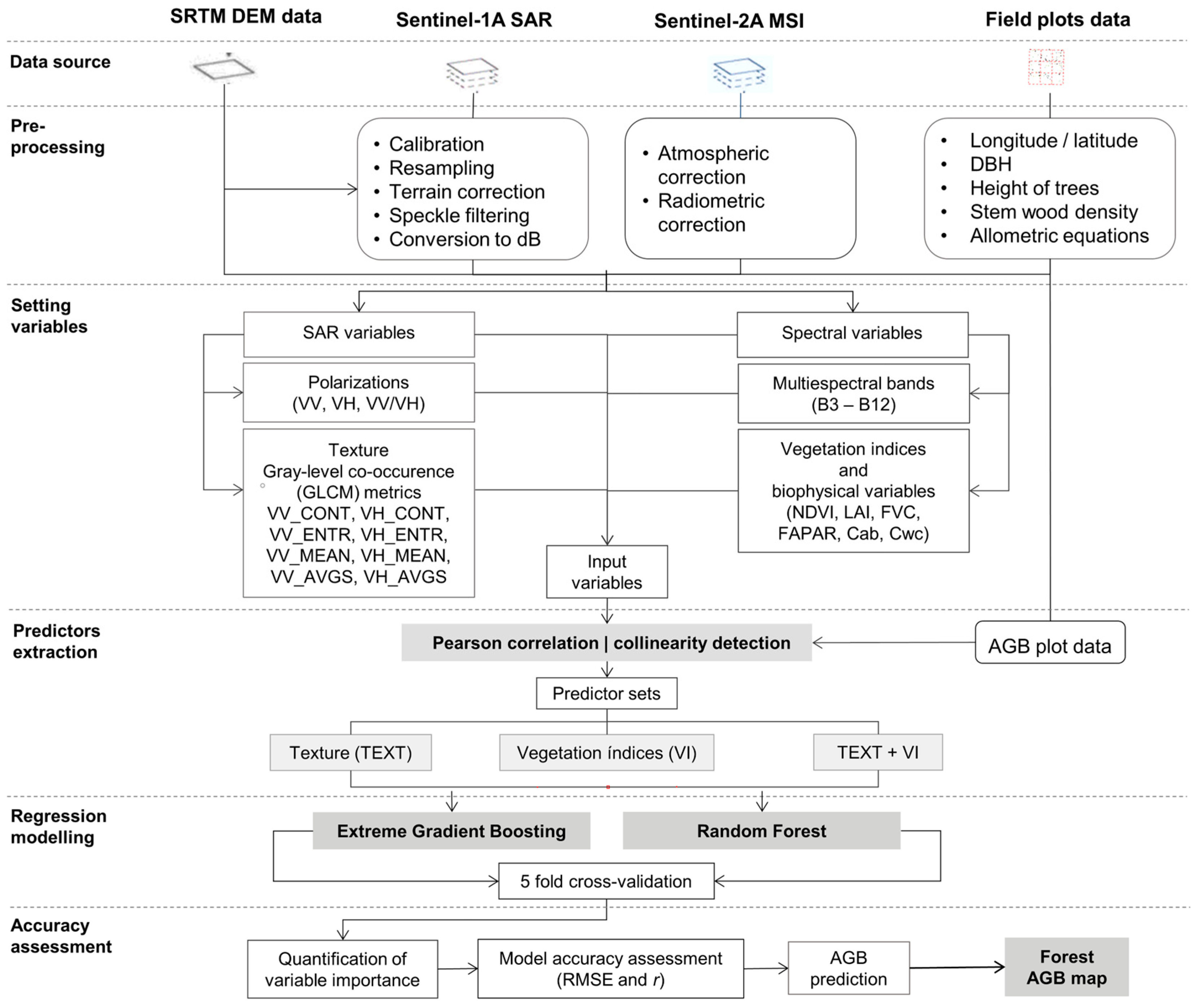
2. Materials and Methods

2.1. Study Area

The study was conducted in the upper Magdalena River valley region, located in the northern part of the Tolima department, Colombia, covering nearly 8000 ha (Figure 1). The region represents the second largest extent of the Colombian dry tropical forest life zone covered by highly fragmented mosaics of secondary vegetation [56]. The geographical extent of the area lies between latitudes 05°11′00″N and 05°04′03″N and longitudes 74°49′18″W and 74°45′43″W. The region has a varying terrain topography, resulting in different conditions from flat plains to steep hillsides. The elevation varies between plot areas and shows a degree slope of 5.72° C-Plana, 11.46° Tambor, 16.18° C-Loma, and 6.30° Jabiru.

According to the classification of [57], the regional climate is flanked by a hot and dry season, which leads to water deficiency [57]. Mean annual temperature is 26.8 °C with a maximum monthly mean of 29.8 °C from July to September [58]. The rainfall regime is characterized by a dry and a wet period (averaging from 831 to 2268 mm per annum, respectively). During the dry season, which lasts from June to September [58], more than 50% of all tree species drop their leaves.

The methodological framework of the study consisted of the following six steps: (1) data source; (2) pre-processing of Sentinel SAR and MSI imagery; (3) setting and adjustment of SAR and spectral variables; (4) extraction of predictor sets; (5) modeling of random forest and extreme gradient boosting regressions; and (6) accuracy assessment and comparison of forest AGB prediction models. Figure 2 summarizes the methodological steps of this study, which are described in detail in the following sections (Section 2.2, Section 2.3, Section 2.4, Section 2.5, Section 2.6 and Section 2.7).

2.2. Data Sources

2.2.1. Field Dataset and Allometric Equation Estimation

Four (4) long-term forest inventory plots, 1 ha each, were set out as part of the Colombian TDF socio-ecological monitoring platforms [59], led by the Alexander von Humboldt Institute in conjunction with several institutions (Figure 1). The plots were spatially clustered across secondary forests containing three distinct stages of recovery aged between 30 and 70 years (

Table 1. Plot ID, forest successional status, number of subplots, number of individual trees >15 cm diameter breast height per subplot, and mean aboveground biomass (Mg/ha⁻¹).

Forest Stand Plot ID	Forest Stratum	Stage of Recovery	Number of Subplots	# of Trees > 15 cm DBH	Mean AGB (Mg/ha−1)
C-Plana	Degraded	>30 Yr.	25	205	63.21
C-Loma	Low degraded	>40 Yr.	25	302	92.21
Tambor	Low degraded	>60 Yr.	25	185	133.65
Jabiru	Degraded	>30 Yr.	25	324	77.39

).

Field data were collected between 2014 and 2015. The locations of all four corners of each plot were determined using a Garmin^® eTrex 10 GPS receiver. Then, the positions (x- and y-coordinates) for all labeled trees were recorded following a standard field protocol of the Forest Dynamic Plots of the Centre for Tropical Forest Science [60]. Later, they were post-processed using ArcGIS (version 10.0, ESRI, RedLands, CA, USA), resulting in a horizontal accuracy of 4–8 m, which is quite common in GPS surveys, with no differential corrections [61] (Figure 1). After, stem diameters (DBH) were measured at 130 cm from the ground or above trunk deformities if present [60]. Total height and tree species were recorded for all standing stems with a DBH ≥ 2.5 cm, including wood-specific gravity (stem wood density (p)) in grams per cubic centimeters.

The AGB (Kg/ha⁻¹) values for single trees within the 4 plots were computed by using the allometric equation for tropical dry forest recommended by [62]:

$$\mathrm{Aboveground} \mathrm{biomass} (\mathrm{AGB})={\mathrm{e}}^{(-2.977+0.916 \ast \ln \left(p \ast DBH2 \ast H\right))}$$

(1)

In this equation, p refers to specific wood density (wood-specific gravity), where data per species in the 4 plots (for a pool of 91 species) were provided by Humboldt monitoring plots. This allometry was computed for every individual tree in our plots. The computed AGB values for the plots varied between 63.21 Mg/ha⁻¹ and 133.65 Mg/ha⁻¹ (Table 1. See the complete list of species present in the plots in Supplementary Material A, Table S1).

2.2.2. Remote Sensing Data Acquisition

Imagery from two satellites (S-1 SAR and S-2 MSI) was used. S-1, carrying a polarized SAR interferometric wide swath mode, operating at C-band (5.405 GHz) with an incidence angle of between 20° and 45°, has opened new opportunities for remote forest AGB estimations by the use of backscatter values at dual polarizations (HH + HV or VV + VH). S-1 data have a 12-day revisit period at the global scale, a spatial resolution of 5 m, and coverage data up to 400 km. The S-1 images in single polarization (VV) and dual polarization (VV and VH) that covered the study area were employed during the time that most closely coincided with the plot measurements dates on 19 May 2015 and 27 November 2015, in dry and wet seasons, respectively (

Table 2. List of S-1–2 imagery acquired for the study.

Mission	Observation Date/Season	Cloud Cover (%)	Cell Size (m)	Unit Resource Identifier (URI)
S-1A	19 May 2015 Dry	-	10	S1A_IW_GRDH_1SDV_20150519T231327_20150519T231352_005997_007BAA_3573
S-1A	27 November 2015 Wet	-	10	S1A_IW_GRDH_1SDV_20151127T231352_20151127T231417_008797_00C8C4_2024
S-2A	21 December 2015 Wet	7	10	S2A_MSIL1C_20151221T153112_N0201_R025_T18NWL_20151221T153112
S-2A	18 June 2016 Dry	5	10	S2A_MSIL1C_20160618T152642_N0204_R025_T18NWL_20160618T153021

).

Cloud-free S-2A data were collected to generate vegetation indices. The S-2 satellite carries a state-of-the-art multispectral imagery instrument with 13 spectral bands covering visible, near infrared (NIR), red-edge (RE), and shortwave infrared (SWIR) wavelengths at 10, 20, and 60 m resolution and a revisit period of 6 days. Here, 60 m (bands 1, 9, and 10) were excluded as they are used to detect atmospheric features. The acquisition dates for the study area were 21 December 2015 and 18 June 2016, in wet and dry seasons, respectively. In addition, selected images were limited to those with cloud cover <10%. S-1 and S-2 images from the European Space Agency were downloaded from the Copernicus Open Access Hub Portal provided by the ESA (https://sentinel.esa.int/web/sentinel/missions/sentinel-1, accessed on 20 June 2020). The acquisition date of the image (18 June 2016) was chronologically very close to Sentinel imagery and close to the dates of the fieldwork, which facilitates a comparison with the field measurements.

2.3. Data Pre-Processing and Setting Variables

2.3.1. SAR Texture Data Processing

Sentinel application platform (SNAP) software (version 6.0, European Space Agency) was used for preliminary processing of S-1 images from wet and dry seasons. The work process of SAR imagery based on S-1 consisted of five steps: (i) radiometric calibration of the different observation dates to obtain the backscattering coefficients, (ii) resampling images to a pixel size of 20 m, closely matching the subplot sizes taken for the field measurements, (iii) speckle filtering based on a Gamma MAP Filter with a window size of 9 × 9 pixel to reduce speckle noise in vegetated areas and increase accuracy [63,64], (iv) terrain correction, based on the 30 m Shuttle Radar Topography Mission (SRTM) digital elevation model (DEM) to geocode and rectify images, and (v) linear conversion into a decibel (dB) unit to generate polarization variables (VH and VV).

SNAP 6.0 software was also used to calculate texture metrics from the geocoded and rectified images of each polarization. Texture features describe the spatial values of variations in pixel brightness (grayscale) at a given offset in an image. The accuracy of AGB estimation is significantly affected by window size. Therefore, when extracting texture features, we need to select the appropriate window size [65]. We experimented with different window sizes and numbers of gray levels. We found that a window size of 3 pixels produced binary outputs, while a window size of 7 pixels was impractical. The appropriate arrangement was found with a sliding window size of 5 pixels and 20 gray levels for the 20 m resampled resolution images (S-1). Texture variables for the VH and VV polarization image were then computed using gray level co-occurrence matrix (GLCM) algorithms [66], and spatial features of the grayscale were extracted using the relationship of the brightness values between the central pixel and its neighborhood within a 5 × 5 pixel moving window. Here, ten texture features were considered: (1) dissimilarity, (2) angular second moment (ASM), (3) contrast (CON), (4) entropy (ENT), (5) homogeneity (HOM), (6) energy (ENE), (7) maximum probability (MAX), (8) GLCM mean, (9) GLCM variance, and (10) GLCM correlation for each of the bands (Table 2).

2.3.2. Multispectral Data Processing

The multispectral images from S-2 (wet and dry seasons) were first atmospherically corrected using the Stand Alone Tool Sen2Cor plug-in (version 2.5.5) of the SNAP toolbox and ATCOR-2 [67] processor. Next, nine reflectance bands with 10 m and 20 m spatial resolution were processed and bands with 10 m were resampled to 20 m using the nearest neighborhood method. Five standard biophysical variables were computed, including leaf area index (LAI), fractional vegetation cover (FVC), fraction of photosynthetically active radiation (FAPAR), chlorophyll content of the leaf (Cab), and canopy water content (Cwc). Finally, the images were computed to obtain the normalized difference vegetation index (NDVI). The equations for band arithmetic used can be found in Supplementary Material B, Table S2.

2.4. Extraction of Predictor Variables (Plot-Level Variable Extraction from Remotely Sensed Data)

To establish the relationship between forest plots and predictor variables, a corresponding predictor pixel value for each plot should be correctly extracted. One approach is to establish a radius buffer around each plot, averaging their pixel values to reduce the effect of the surrounding locations [3,17,19]. Our sampling approach was a split plot design, i.e., dividing the 1 ha plots into 25 subplots of 20 m × 20 m. Different subplot sizes were previously tested, but the chosen size of 20 m contained the best trade-off between radiometric–spectral accuracy and loss of spatial information and is similar to the one used for the Sentinel estimations. So, the effect of the surrounding areas is minimized, because the intrusion of surroundings (tree canopies in our case) is embedded by the neighboring subplot. Therefore, we first generated a center coordinate (or centroid) of each subplot. Pixel values for texture and multispectral types were then extracted for each subplot centroid. The AGB values estimated at each subplot were aggregated by totaling the AGB of all individual trees, so that each raster of texture and multispectral types coincided with an individual pixel.

Each 1 ha plot then coincides with approximately 25 textured and spectral pixels, resulting in 100 extracted pixel values for AGB analysis. This ensured representative sampling and facilitates a robust comparison between plot AGB data and the Sentinel imagery. The total number of predictor variables available for AGB modeling was 70. In order to differentiate and identify more suitable predictor variables to obtain higher model accuracy, texture and spectral vegetation variables were composed as follows: separately and in combination, i.e., three predictor sets 1 (TEXT), 2 (VI), and 3 (TEXT-VI) (Figure 1).

2.5. Predictor Variable Reduction and Selection

Although a total of 70 explanatory variables (40 TEXT and 30 VI) were extracted, not all of them contributed to the AGB regression models. It is therefore important to identify the predictor subsets to simplify the model and eliminate variables that are not related to plot-based AGB and that are collinear with each other. In order to identify such variables, correlation and regression analysis was conducted using the sets TEXT and VI as explanatory variables of the AGB. The statistical analysis was carried out in R using the “corrplot” packages. In the first step, Pearson’s linear correlation coefficient (r) [68] was computed to discard the presence of multicollinearity and to detect the statistical relationship between extracted variables within predictor sets and AGB. Here, variables were confirmed for inclusion only if they were uncorrelated or weakly correlated (either p-value > 0.05 or r < 0.4 for significant correlations). Secondly, a stepwise variable selection method was performed using the “stepAIC” function as implemented in the “MASS” package to reduce redundant information, so as to identify the best subset mixture of variables and the optimal models. The stepwise procedure in this study starts by establishing an AGB estimation model, containing the candidate variables from the initial Pearson’s linear correlation coefficient (r) selection, to only include correlated variables to AGB. Then, the least important predictor variables whose p-value was above the threshold (0.05) were successively removed from the model, and the smallest subset of predictor variables were considered for constructing the final RF and XGBoost models. A detailed process for selection of variables is provided in Table 3 and in Supplementary Material C, Figure S1.

2.6. Data Analysis (Statistical and Regression Algorithms for Modeling AGB)

With the aim of (i) identifying important predictor variables, (ii) testing the efficiency of the predictor sets (TEXT, VI, and TEXT-VI), and (iii) comparing the predictive accuracy of different regression methods for the estimation of AGB, two ensemble regression algorithms were analyzed: the random forest (RF) model and extreme gradient boosting (XGBoost) model. In each model, the predictor sets were considered to be independent variables and AGB was the dependent variable. All models were performed in the R statistical software (version 4.0.3) environment and the procedures are briefly described below.

2.6.1. Random Forest Regression Model

RF is an ensemble machine learning algorithm based on the tree decision proposed by Breiman [69]. It can now be used routinely as a regression algorithm in many scientific fields and it has been used for response variables in different-scale regression-based spatial applications such as forest AGB in the tropics [31,70,71,72]. This ensemble learning method is a useful technique, which offers the advantage of being non-parametric, dealing with dimensional data problems (here, ground data paucity), and preventing the overfitting of models [73]. The algorithm is based on multiple decision trees fitted to random subsets of the training sample. Decision trees are generated using a randomly selected 2/3 of the original sample data to train the trees with bootstrap aggregation, i.e., re-sampling the data many times with replacement (bagging). The rest of the data, i.e., the remaining third, are called out-of-bag (OOB) data, and they are not seen by the model and are used as validation samples to estimate the model errors [69,72]. At each node of the tree, a set of predictor variables are chosen randomly to identify the most efficient splits, making the model performance immune to the problem of overfitting [69]. Therefore, three important parameters need to be adjusted, ntree (the number of trees to achieve a desirable prediction), mtry (the number of different predictor samples at each split), and min_n (the minimum number of data points in a node required for additional splits) [69,74].

Here, the RF regression process was performed using the “randomForest” package. Since our plot numbers were limited, we did not conduct a fully independent validation [75] but relied on spatial internal cross-validation [76] as an adequate evaluation model. A 5-fold spatial internal cross-validation approach was fitted using this partitioning for more persuasive results. Within this process, one subset at a time was used as a test set, while the other three were used as training sets for a predictive model [77]. The tuneRF function was used to identify the optimal mtry and ntree values. Therefore, the models were generated with an interval value of ntrees between 90 and 100, while mtry varied in intervals between 5 and 7, which optimally explained the predictor variables. Detailed tuning parameters and the fitting process of mtry and ntrees are displayed in Supplementary Material D, Table S3 and Figure S2. To evaluate the importance of each variable, the “randomForest” package also has two indices to measure variable importance: the first measurement is the percent increase in mean square error (%IncMSE), which is computed from permuting OOB data; and the second score is the total decrease in node impurities from splitting up the variable (IncNodePurity), which is measured by the residual sum of squares. Therefore, in both indices, a higher score indicates that the variable is important in the model and in explaining variability of the response variable, whereas values near zero indicate the variable is not important [78].

2.6.2. Extreme Gradient Boosting Model

XGBoost is another ensemble learning technique based on the gradient boosting framework, proposed by Chen and Guestrin [79] to improve the predictive performance of regression or classification problems [80]. Unlike RF, XGBoost combines the advantages of both bagging and boosting, where it can correct the residual error to generate a new tree based on the previous tree [81]. Like the boosted regression trees [82], it follows the principle of gradient enhancement; however, more regularized model formalization is applied to XGBoost to control overfitting, making it more accurate. Additionally, the XGBoost algorithm works in parallel with all available computing cores in combination with the regularization factor to produce a prediction rule faster than most other tree boosting methods [79]. In fact, their approaches have received attention for mapping purposes in RS [30] due to the extraordinary fitting flexibility and statistical modeling properties. The implementation of XGBoost involves a parameter-tuning process that helps to maximize the performance of the model in terms of both speed and predictive accuracy. The most important parameters of XGBoost include: (1) nrounds, which is the maximum number of boosting iterations. (2) max_depth is the maximum depth of an individual tree. (3) colsample_bytree is the subsample ratio of columns. (4) eta is the learning rate and is used during updating to prevent overfitting. (5) gamma is the minimum loss reduction required to make a further partition on a leaf node of the tree. (6) min_child_weight is the minimum sum of instance weight needed in a leaf node (7) subsample is the subsample ratio of the training instance or rows.

Here, we implemented the XGBoost regressor from the “xgboost” open-source R package [51]. The tuning grid approach was used to find the best combination of parameters. After the tuning grid has been refined several times and a certain number of iterations have been completed, the range of parameters with the best combination set for prediction on holdout test data is selected as follows:

• For nrounds = from (245 to 420);
• For learning_rate values, eta = (0.009 to 0.03);
• For max_depth = from (3 to 5).

The optimal tree specific parameters are determined:

• For min_child_weight = from (0.4 to 0.9);
• For subsample = from (0.3 to 0.8);
• For colsample_bytree = from (0.3 to 0.7).

The regularization parameter is set:

• For gamma = from (0 to 10).

Detailed processes for tuning parameters of the XGBoost regression are provided in Supplementary Material D, Table S4 and Figure S3. To compare the stability of the results over all datasets, the xgboost package also has two indices to evaluate the variable importance for each of predictor’s set variables, first by computing the fractional contribution of each feature to the model based on the total gain of these variables’ splits (Gain) and secondly by computing the relative number of times a feature is used in trees (Frequency) (XGBoost: [51]). We use different evaluation metrics to measure the performance of the selected optimized XGBoost model on hold out test data.

2.7. Model Accuraccy Assessment of Estimated AGB

In order to evaluate the performance of the predictor’s sets and models in estimating AGB, our study used a 5-fold cross-validation for modeling training and validation. To this end, we used the coefficient of determination (R²) to account for goodness-of-fit to the training data and the root mean square error (RMSE) and relative RMSE (%) to assess accuracy of the models. They are defined according to

$$R^2=1-\frac{{\sum }_{i=1}^N (y_i-{{\widehat{y}}_i)}^2}{{\sum }_{i=1}^N (y_i-{\overline{y}}_i{)}^2}$$

(2)

$$\mathrm{R}\mathrm{M}\mathrm{S}\mathrm{E}=\sqrt{ \frac{1}{N}\sum _{i=1}^N({{\mathrm{P}\mathrm{R}\mathrm{E}}_i-{\mathrm{O}\mathrm{B}\mathrm{S}}_i)}^2}$$

(3)

$$\mathrm{R}\mathrm{M}\mathrm{S}\mathrm{E} (\mathrm{\%})=100\times \frac{\mathrm{R}\mathrm{M}\mathrm{S}\mathrm{E}}{{\mathrm{O}\mathrm{B}\mathrm{S}}_{\mathrm{m}\mathrm{a}\mathrm{x}}-{\mathrm{O}\mathrm{B}\mathrm{S}}_{\mathrm{m}\mathrm{i}\mathrm{n}}}$$

(4)

where N is the number of plots, PRE_i and OBS_i denote the ith predicted and observed values, respectively. RMSE (%) is the RMSE divided by the range of observed values of a predictor set variable being predicted. The value is often expressed as a percentage, where lower values indicate less residual variance. Additionally, the relative RMSE (%) was defined as RMSE/mean (OBS) × 100.

The relative RMSE was used to compare the performances across the different machine learning algorithms and the statistical techniques. Generally, the performance of the model was estimated by comparing the differences in R² and RMSE of the observed-versus-predicted value plots. Higher R² and lower RMSE values, respectively, corresponded to the higher precision and accuracy of a model for predicting forest AGB. Based on these statistics, along with observed-versus-predicted AGB graphs, the most accurate model (in this case, RF) was used to construct a regular 20 m resolution AGB map in the study area. Next, the predictive map was derived from TEXT and VI predictor variables combined using the “raster” and “randomForest” packages through R statistical software (version 4.2.0).

3. Results

3.1. Selection of Variables

Of the 40 predictor variables (see Supplementary Material B, Table S2) derived from S-1 SAR imagery, only 16 variables were significantly correlated with AGB plot (AGB—S-1) (Table 3), based on critical values for Pearson’s correlation and stepwise regression (Supplementary Material C, Figure S1), and 9 predictor variables out of 30 (see Supplementary Material B, Table S2) derived from S-2 MSI (AGB—S-2).

Table 3. Statistical results of the linear stepwise regression method for the best selected variables from S-1 and S-2 imagery with AGB.

(S-1) SAR Texture Set			(S-2) MSI Set
Variable	Coefficient	Correlation with AGB. r	Variable	Coefficient	Correlation with AGB. r
Intercept	2.20	------	Intercept	−12.61	------
D_VH_GLCMMean	−8.341	−0.28 ***	D_B3	168.29	−0.07 ***
D_VH_GLCMCorr	1.92	−0.22 **	D_B7	−39.79	0.12 **
D_VV_Cont	−3.83	0.10 ***	D_lai	9.69	0.23 *
D_VV_GLCMMean	−5.12	−0.11 ***	W_B6	224.54	0.32 ***
D_VV_GLCMVari	−4.90	−0.12 ***	W_B7	−61.56	0.40 **
D_VH_ASM	8.52	−0.16 **	W_B8A	−301.76	0.42 ***
D_VH_Dis	2.20	0.15 **	W_B11	389.02	−0.20 ***
D_VV_Ent	−3.28	0.15 **	W_cab	0.13	0.48 ***
D_VV_MAX	5.13	−0.13 *	W_cw	469.03	0.50 ***
D_VV_Ene	3.52	−0.14 *
W_VV_GLCMMean	−8.45	−0.20 **
W_VV_GLCMVari	4.25	−0.21 **
W_VH_Dis	4.90	0.12 *
W_VH_GLCMCorr	3.19	−0.18 *
W_VV_Hom	7.75	−0.19 *
W_VV_Ent	3.39	0.19 *

The significance level is quantified by * p-value < 0.05; ** p-value < 0.01; *** p-value < 0.001.

Table 3. Statistical results of the linear stepwise regression method for the best selected variables from S-1 and S-2 imagery with AGB.

(S-1) SAR Texture Set			(S-2) MSI Set
Variable	Coefficient	Correlation with AGB. r	Variable	Coefficient	Correlation with AGB. r
Intercept	2.20	------	Intercept	−12.61	------
D_VH_GLCMMean	−8.341	−0.28 ***	D_B3	168.29	−0.07 ***
D_VH_GLCMCorr	1.92	−0.22 **	D_B7	−39.79	0.12 **
D_VV_Cont	−3.83	0.10 ***	D_lai	9.69	0.23 *
D_VV_GLCMMean	−5.12	−0.11 ***	W_B6	224.54	0.32 ***
D_VV_GLCMVari	−4.90	−0.12 ***	W_B7	−61.56	0.40 **
D_VH_ASM	8.52	−0.16 **	W_B8A	−301.76	0.42 ***
D_VH_Dis	2.20	0.15 **	W_B11	389.02	−0.20 ***
D_VV_Ent	−3.28	0.15 **	W_cab	0.13	0.48 ***
D_VV_MAX	5.13	−0.13 *	W_cw	469.03	0.50 ***
D_VV_Ene	3.52	−0.14 *
W_VV_GLCMMean	−8.45	−0.20 **
W_VV_GLCMVari	4.25	−0.21 **
W_VH_Dis	4.90	0.12 *
W_VH_GLCMCorr	3.19	−0.18 *
W_VV_Hom	7.75	−0.19 *
W_VV_Ent	3.39	0.19 *

The significance level is quantified by * p-value < 0.05; ** p-value < 0.01; *** p-value < 0.001.

Overall, the (S-2) VI variable set showed the highest correlations. Specifically, W_CW achieved the highest positive correlation, with the AGB plot r = 0.5, followed by W_CAB with a positive correlation of 0.48. Among the set of S-1 SAR texture variables, the D_VH_GLCMMean achieved the highest negative correlation coefficient, with the AGB plot obtaining an r-value of −0.28. This was followed by D_VH_GLCMCorr, with an r-value of −0.22. These results indicate that the performance of these two sets of variables was optimal as the number of variables decreased. It should also be noted that individual SAR polarization metrics (VH and VV) were not included in the analysis, as the results were not always satisfactory with R² < 0.05, regardless of the prediction method used.

3.2. Comparison Analysis of the AGB Models

3.2.1. RF and XGBoost Regression Model Performance

Optimal variables were selected and sorted into two predictor sets, namely (S-1) TEXT and (S-2) VI, as explained in Section 3.1 and Section 2.4. The accuracy of the RF and XGBoost regression algorithms in estimating AGB was analyzed and compared using R² and RMSE measurements obtained through fivefold cross-validation, based on parameter tuning (see Supplementary Material D).

Table 4. A comparison of the accuracy of RF and XGBoost models based on predictor sets is presented both individually and in combination. We reported the R² coefficient of determination between the observed and estimated AGB, as well as the RMSE in Mg/ha⁻¹ of AGB using 5-fold cross-validation conducted on the training and testing datasets.

Model Abbrev.	Predictor Sets		Training Dataset		Testing Dataset
			R2 Observed vs. Estimated	Cross-Validation RMSE (Mg/ha−1)	R2 Observed vs. Estimated	Cross-Validation RMSE (Mg/ha−1)
RF	(S-1)	TEXT	0.83	31.03	0.64	46.10
	(S-2)	VI	0.79	40.30	0.70	45.44
	(S-1 + S-2)	TEXT-VI	0.81	38.60	0.78	42.25
XGBoost	(S-1)	TEXT	0.71	41.75	0.43	50.53
	(S-2)	VI	0.62	45.90	0.57	52.95
	(S-1 + S-2)	TEXT-VI	0.73	40.60	0.60	48.41

provides a summary of the accuracy findings for the predictor sets during training and testing phases, both individually and when combined. According to the 5-fold cross-validation of the XGBoost model, (S-1) TEXT and (S-2) VI predictor sets performed inefficiently in estimating AGB. On the other hand, the findings suggest that both predictor sets, (S-1) TEXT and (S-2) VI, performed better in predicting AGB when using the RF algorithm. Evaluating the measurements against the dataset criteria individually, it was determined that the (S-2) VI predictor set, instead of (S-1) TEXT, produced slightly more accurate results (RMSE = 45.4 Mg/ha⁻¹, R² = 0.70) when compared to the results of the (S-1) TEXT predictor set on the testing dataset (RMSE = 46.1 Mg/ha⁻¹, R² = 0.64), as shown in Table 4.

Moreover, the results indicate that the combination of (S-1) TEXT and (S-2) VI predictor sets enhances the estimation accuracy of both algorithms (RF and XGBoost) by increasing the R² and reducing the RMSE, compared to individual predictions (refer to Table 4). The R² increased by 0.18 while the RMSE decreased by 6.16 Mg/ha⁻¹ with the RF model (TEXT-VI), which is better than the XGBoost model (TEXT-VI). In general, the RF model and the combined predictor sets (TEXT-VI) demonstrated the best performance.

To demonstrate the predictive ability of both the RF and XGBoost algorithms concisely, were used the tuning parameters (refer to Supplementary Material D) to validate and estimate all six models. The scatterplot distribution can be observed by fitting and plotting the predicted and observed AGB values on the test datasets (Figure 3), which enables the comparison of differences and correlations between the estimated and observed AGB values. For training datasets, please refer to Supplementary Material E. Generally, the scatterplot shows that the data points form a densely clustered and aligned pattern along a straight line. This implies that the predictions are reasonably accurate (Figure 3).

Furthermore, some data points exhibited a moderate pattern of dispersion, potentially due to external factors. If validated, conducting a more detailed examination of these outliers may assist in identifying their relationships with other factors. The RF model estimates were more clustered around the centerline (depicted by a 1:1 gray solid line) compared to the XGBoost models (R² RF > R² XGBoost), signifying improved accuracy. These results indicate a significant correlation between the estimated and observed AGB values, suggesting the model’s potential as a benchmark for managing forest resources and conducting research on the carbon cycle.

Moreover, the models all showed both overestimation and underestimation. The scatterplots (see Figure 3) reveal that the estimated values surpassed the centerline when the AGB was below 50 Mg/ha⁻¹, whereas it was lower when the AGB was greater than 100 Mg/ha⁻¹. This implies that although the models combined predictor sets (S-1) TEXT and (S-2) VI to reduce estimation errors, they still overestimate AGB values at lower levels and underestimate them at higher levels.

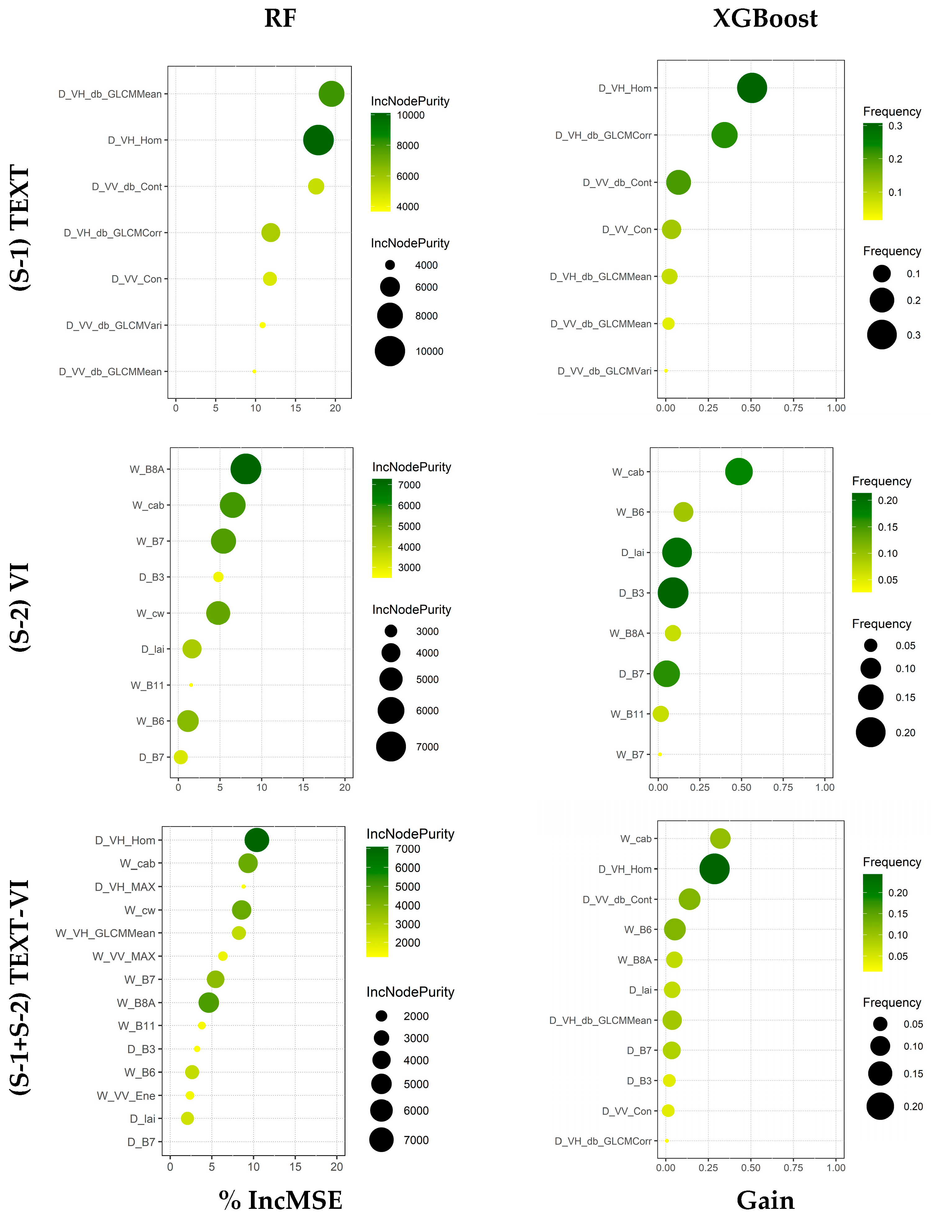
3.2.2. Ranking of Variable Importance for AGB Estimation

To examine the relative contribution of the variables in the predictor set regression models to AGB estimation, we performed additional evaluations of their predictive ability. Figure 4 shows the ranking of the most important variables given by the RF and XGBoost models, as derived from %IncMSE and gain measures.

The size and color of the circles represent the IncNodePurity for the RF-based models and frequency for the XGBoost-based models, respectively. This reflects the comprehensive ability of the variables to estimate AGB, demonstrated for both types of importance. Our analysis of variable importance using the RF-based and XGBoost-based models revealed that three variables had a significant effect on AGB in all three datasets. These variables are D_VH_Hom, D_VH_db_GLCMMean, and W_cab, as shown in Figure 4. However, there was a difference in the order of the variables ranked in the predictor sets by both algorithms. For the (S-2) VI spectral dataset, both the XGBoost-based and RF-based models showed the significance of W_cab, ranking it first and second, respectively, but it should be noted that the W_B8A was highly significant and secured the first rank in the RF-based model. Concerning the (S-1) TEXT dataset, D_VH_Hom exhibited a high correlation with AGB when compared to the other notable D_VH_db_GLCMMean variable. Regarding the combined datasets, it is noteworthy that the (S-1) TEXT variables hold greater importance than the (S-2) VI spectral variables, implying a significant improvement in the model’s performance due to the inclusion of dry season (S-1) TEXT variables (see Figure 4). These results align with the scatterplot outcomes (see Figure 3).

3.3. Mapping of Estimated Forest AGB

Finally, the RF model was utilized to estimate a 20 m resolution map of forest AGB in the combined (S-1) TEXT and (S-2) VI dataset with optimized variables. Figure 5 exhibits the estimated map with AGB values ranging from a minimum of 28.8 Mg/ha⁻¹ to a maximum of 335 Mg/ha⁻¹ and an average of 92 Mg/ha⁻¹. It is noteworthy that around 70% of the study area demonstrates AGB values in the range of 70 to 100 Mg/ha⁻¹.

Figure 5 illustrates that the spatial distribution patterns of the AGB map coincide with the forest distribution in the study region. The zones with high estimated AGB values were identified as dense forest areas, mainly situated in isolated and narrow patches with steep slopes. In contrast, areas with significant agricultural impact on flat terrain exhibited low estimated AGB values (Figure 5). In certain instances, there was a minor overestimation or underestimation of AGB in areas with either sparse or dense forests. However, these discrepancies were in line with the study area, where 70% of the AGB map ranged from 70–100 Mg/ha⁻¹. Other vegetation coverage types such as herbs, crops, and shrubs were not included in this research; therefore, the estimated AGB should be viewed as conservative but still indicative of the fundamental AGB status of TDFs. Currently, Colombia’s AGB estimation system is incomplete, but this study offers a reliable approach for estimating regional AGB.

4. Discussion

Within the present study, our aims were fourfold: firstly, to evaluate the performance of two ensemble learning regression methods that use different predictor sets; secondly, to determine the potential of Sentinel imagery for estimating AGB; thirdly, to identify the optimal predictor variables; and lastly, to illustrate that valid spatial estimates of forest AGB can be attained in the complex TDF region with limited forest plot data, by appropriately selecting critical predictor variables and achieving optimal performance.

4.1. Model Performance: Efficiency of the RF and XGBoost Using Predictor Set

Based on the predictor selection implemented in Section 3.1, we have selected 25 potential options from the initial 70 variables in order to evaluate the performance of the ensemble regression techniques in estimating AGB. The selection of potential predictors is critical for machine learning methods, as it preserves the most general relationships of the spectral and geometric feature space from a theoretical perspective. Accordingly, we compared two machine learning methods—the RF and XGBoost models—using the 25 variables selected from the predictor sets (S-1) TEXT and (S-2) VI. Among the two techniques evaluated, our results showed that RF, using the combined predictor sets TEXT and VI, achieved the highest accuracy with R² = 0.78 and RMSE = 42.25 Mg/ha⁻¹, outperforming XGBoost in all cases (Figure 3).

Many previous studies have shown that the RF method performs better when using combined datasets to estimate AGB [35,51], which our own research supports. For instance, in a comparable recent study conducted in a dryland forest ecosystem, David et al. [39] combined (S-1) SAR and (S-2) VI to estimate and map AGB. Their results demonstrate that the RF approach was more accurate (R² = 0.95, RMSE: 0.25 Mg/ha⁻¹) compared to the linear regression. Another study by Ghosh and Behera [52] employed two machine learning techniques, RF and SGBoost, to estimate AGB using S-1 SAR textures and S-2 VI data. The study found that when both (S-1) SAR and (S-2) VI were combined, the RF method was the most accurate (R² = 0.74, RMSE = 82.6 Mg/ha⁻¹). In a similar study, Chen et al. [51] compared RF with several other techniques (SWR, GWR, ANN, SVR) to estimate AGB using (S-1) SAR and (S-2) VI. The study demonstrated exceptional overall prediction accuracy and robustness (R² = 0.97, RMSE = 61.1 Mg/ha⁻¹).

However, it is important to note that differences in accuracy were observed between our findings and those of David et al. [39], Ghosh and Behera [52], and Chen et al. [51], as evidenced by the differences in RMSE and R² values. The dissimilarities in accuracy achieved could be explained by distinct factors. Initially, our study implemented a spatially clustered plot design (Section 2.2.1 and Section 2.4), which is atypical for estimating AGB. This design may have a tendency to overrepresent the most intricate vegetation, leading to uncertainty in AGB estimation [83]. Additionally, the study area contains a varied vegetation cover, and TDFs are characterized by considerable complexity in forest structure and tree species composition. Furthermore, our methodology did not employ site-specific allometric equations to estimate AGB, as they are not available for the study area. Therefore, it is possible that the AGB reference data may be uncertain due to significant variations in values for certain tree species. Thirdly, the AGB for our TDF is relatively low. The field mean AGB observed was 92 Mg/ha⁻¹, which is less than half of the 281 Mg/ha⁻¹ reported by Ghosh and Behera [52] in the Terai forest ecosystem and lower than the 124 Mg/ha⁻¹ reported by Chen et al. [51] in a deciduous broadleaved forest ecosystem. The average AGB of 51 Mg/ha⁻¹ as reported by David et al. [39] in a dryland forest ecosystem is reasonably close. The differences in model estimation accuracies between our research and those previous studies may also be partially explained by variations in the study area location, tree species phenology, and forest ecosystems. Overall, the RF method effectively modeled the complex and non-linear correlations between predictor variables and AGB in our TDF study area. This was achieved by utilizing the advantages of both the forest plots and RS data. We attribute the suitability of the RF method for estimating AGB to its well-designed modeling approach, which includes predictor selection, and the model´s capacity to tolerate noise and outliers [69,71,74] in heterogeneous ecosystems. In contrast, the XGBoost algorithm has been found to be more sensitive to outliers and noise compared to RF, due to its absence of regularized learners in a sequence of relationships [81]. Although regularization mitigates the problem of overestimation and underestimation, complete elimination is unfeasible when relying on machine learning algorithms [18].

4.2. Potential of Sentinel Imagery Combination for Estimating AGB

Our findings suggest that relying only on S-1 or S-2 data is insufficient for achieving the desired level of accuracy for estimating AGB. However, S-2 data are comparatively more suitable for this purpose as compared to S-1 data. These findings are consistent with prior research that has evaluated the efficacy of SAR and optical data for estimating AGB [30,31,52,84]. However, other studies have reported contrasting outcomes [35,85]. This disadvantage may arise as C-band SAR is limited in its ability to obtain vertical structural details of complex forests, particularly when compared to longer waves such as L-band and P-band. Previous studies have demonstrated that S-2 data have the potential to improve the accuracy of AGB estimation when compared with S-1 data. Forkuor et al. [84] evaluated S-1 and S-2 data for predicting forest AGB and concluded that S-2 data produced more accurate estimates. Similarly, Castillo et al. [34] have reported that using LAI from S-2 models results in a higher level of accuracy when compared to raw bands (S-1 and S-2) and VI. Our results highlight the importance of using S-2 data as a reliable predictor for AGB estimation, whilst the relatively inferior penetration capacity of S-1 data solely makes it unsuitable for the study location.

Therefore, combining SAR and optical data to calculate parameters for estimating forest AGB is a pioneering approach. Ongoing research has illustrated the effectiveness of this approach in improving the accuracy of sensor data combination for AGB estimation. In their study, David et al. [39] successfully combined S-1 C-band SAR imaging with S-2 MSI to map AGB data of the dryland forests in a national park in Botswana. The analysis showed a significant correlation between AGB and the combined Sentinel imagery. In a previous study conducted by Ghosh and Behera [52], the AGB of tropical forests was assessed by using S-1 C-band SAR backscatter and S-1 data textures, as well as VI from S-2 data. The results demonstrated that combining SAR backscatter and VI produced the most accurate outcome. Other studies, for instance the ones conducted by Chen et al. [35,51], employed backscatter coefficients and textures from S-1 in conjunction with VI from S-2 to estimate the AGB of temperate forests in China and achieved successful results. The effectiveness of these estimations can largely be attributed to the complementary nature of the data characteristics (i.e., each sensor detects different phenomena) and imaging processing techniques [11]. This indicates that integrating multisensor data have potential in improving the accuracy of AGB estimations.

Furthermore, valuable insights can be gained by incorporating SAR and optical data collected during different seasons to estimate forest AGB by combining S-1 and S-2 images. Our analysis of seasonal dry forests indicated that the most accurate AGB estimates were obtained by combining both S-1 and S-2 predictor sets (see Table 4 and Figure 3). It should be noted that the amount (or proportions) of vegetation in dry forests vary seasonally due to phenological changes [86]. Specifically, this study considers the leaf-on condition during the wet season and the leaf-off condition in the dry season. From this, it can be deduced that the S-1 C-band SAR signal, which is more receptive to the leaf-off conditions, contains essential information that is missing from the S-2 optical MSI data during the dry season. While the S-1 C-band SAR data omit critical information about leaf-on conditions during the wet season [84], the S-2 optical MSI is more responsive to these conditions. Nonetheless, the combination of the two datasets is advantageous in determining accurate AGB estimations [36,53], as evidenced by this study.

4.3. Important RS Predictor Variables

An importance ranking analysis (Figure 4) was performed to determine the most influential predictor variables for AGB mapping. Since they represent different aspects of the canopy structure, datasets S-1, S-2, and their combination were assessed. Regarding the importance of S-2 variables, specifically the red-edge bands (W_B7, W_8A) and VIs (W_cab, W_cw) during the wet season, it was found that these were the significant variables in our study area (Figure 4), which is characterized by a dense and multilayered canopy. This is consistent with previous research that has found a strong relationship between red-edge VI and AGB, especially in areas with complex stand canopy structures [18,48], such as our study region. For example, Castillo et al. [34] concluded that the S-2 red-edge (B6, B7) and near-infrared (B8, B8A) bands had a higher correlation with AGB than the visible and shortwave infrared bands. In addition, the VIs derived from the red-edge (B5, B6), NIR (B8), and SWIR (B12) bands correlated more strongly with the AGB than any other band combination. Similarly, in the research by Mutanga and Skidmore et al. [18], the red-edge-derived VI showed a stronger correlation with AGB than other spectral bands. This is attributed to the red-edge’s exceptional ability to reflect the complexity of the forest stand structure. In addition, the red-edge bands and derived VIs (such as LAIxCab and LAIxCw) used in conjunction with S-1 SAR data in this study contribute to AGB estimation by reducing saturation issues [86,87,88].

For the S-1 variables, SAR texture, particularly the dry season variable D_VH_HOM, exhibited the most significant potential for explanatory power in the prediction models (Figure 4). This can be explained by the effectiveness of C-band SAR cross-polarized texture features in areas with considerable local variations, such as seasonal influences [36], and their capability to provide more information in multilayered forests with complex structures [19], notably during the dry season, as seen in our case. In a comparable terrain located in tropical West Africa, Laurin et al. [89] conducted forest and land cover mapping using SAR textures and optical data. They determined that cross-polarized textures were the most significant variables in the area, which has a high proportion of deciduous vegetation. During the dry period when branches are visible, textures are crucial. Zhao et al. [90] noted that vegetation types and RS data sources impact textures and that a single texture is not optimal for estimating AGB in various study areas. Our analysis determined that texture features, specifically D_VH_HOM and D_VH_GLCMMean, were the most significant variables for both RF and XGBoost estimation in comparison to spectral bands. These findings are consistent with Lu’s [19] research which emphasizes that texture images are more effective than spectral bands in estimating AGB, especially in forests with complex stand structures. However, this was not observed in the study conducted by Ghosh and Behera [52] on homogeneous sites, where the SAR texture performed worse than the VI.

4.4. Forest AGB Map

Based on our findings, we suggest applying the RF method, which involves combining S-1 SAR and S-2 MSI data, to determine forest AGB in the research region (Figure 5). The AGB map provides accurate representations of biomass distribution patterns in the studied area. The steepest and most challenging forest sections with minimal human intervention have the highest AGB values, ranging from 60 to 100 Mg/ha⁻¹. In contrast, in the flat sections with high levels of agricultural activity, the proportion of AGB is less than 60 Mg/ha⁻¹. Nevertheless, in both areas of study, significant small-scale variations in the spatial distribution of AGB values were detected. The disparities in spatial variability between the RGB S-2 spectra and AGB map (Figure 5A,B) are attributable to the RF model’s predisposition to underestimate small and large AGB values (Figure 3). For instance, numerous steep slope forest AGB estimates display patches of moderate to low pixel values within the AGB map. By contrast, the RGB image spectra reveal that the patches indicate the presence of vegetation cover, possibly due to varying degrees of vegetation density.

Although our study achieved its objectives, there were also unavoidable limitations. One of the issues of our AGB map is its failure to encompass all the vegetation structures in the study area. We did not include the range of various forest age classes, comprising degraded vegetation, as we lacked field reference plot data. We encountered difficulties when attempting to incorporate agricultural zones into our AGB map due to the crops’ significant seasonal variability in the study area and their lack of relevance to our research. More precisely, our model was calibrated with a few reference plots located within well-preserved forest stands, resulting in higher sensitivity to outliers and lower AGB estimates in potentially high AGB areas. Therefore, from a field perspective, if resources become available to enlarge our sampling in the future, we recommend enhancing our sample size for distinct forest classes or types.

5. Conclusions

Accurate estimates and regional mapping of forest AGB distribution are critical for strategic forest planning, REDD frameworks, and carbon modeling. RS data can provide an efficient approach to spatially represent field biomass measurements. Our study shows that freely available Sentinel data can be used in combination with ensemble algorithms to reliably and accurately estimate forest AGB in the TDF region. The accuracy of the AGB estimations obtained in this study corresponds to that reported in comparable studies based on single sensor or combined sensor datasets. The most accurate estimates of AGB were achieved through the application of RF, which combined data from both MSI and SAR textures, based on a limited number of clustered plots. The exceptional predictive capabilities demonstrated by the RF ensemble algorithm highlight the importance of carefully selecting an appropriate set of predictor variables. Furthermore, incorporating red-edge indices and cross-polarized texture variables is important in estimating AGB due to their ability to alleviate saturation effect and considerably enhance model performance. Still, our model performance suggests that there is potential for further improvement in mapping AGB within TDF environments.

Thus, future research should focus on expanding the collection of high-quality field data and developing allometric functions for local tree species to improve the accuracy of ground data and validate TDF results. The use of LiDAR could be considered depending on the assessment scales. In regions with limited forest inventory plots, LiDAR can serve as an extension of inventory plots. Furthermore, as it captures spatial variability and provides accurate assessments of forest characteristics, including stand height and AGB distribution, LiDAR can be an effective way to improve training data for correlation and to complement observations from other RS sources.

References

1. Bonan, G.B. Forests and climate change. Forcings, feedbacks, and the climate benefits of forests. Science 2008, 320, 1444–1449. [Google Scholar] [CrossRef] [PubMed]
2. Mitchard, E.T.A. The tropical forest carbon cycle and climate change. Nature 2018, 559, 527–534. [Google Scholar] [CrossRef] [PubMed]
3. Lu, D. The potential and challenge of remote sensing-based biomass estimation. Int. J. Remote Sens. 2007, 27, 1297–1328. [Google Scholar] [CrossRef]
4. Goetz, S.J.; Hansen, M.; Houghton, R.A.; Walker, W.; Laporte, N.; Busch, J. Measurement and monitoring needs, capabilities and potential for addressing reduced emissions from deforestation and forest degradation under REDD+. Environ. Res. Lett. 2015, 10, 123001. [Google Scholar] [CrossRef]
5. West, P.W. Tree and Forest Measurement; Springer International Publishing: Cham, Switzerland, 2015. [Google Scholar]
6. Bustamante, M.M.C.; Roitman, I.; Aide, T.M.; Alencar, A.; Anderson, L.O.; Aragão, L.; Asner, G.P.; Barlow, J.; Berenguer, E.; Chambers, J.; et al. Toward an integrated monitoring framework to assess the effects of tropical forest degradation and recovery on carbon stocks and biodiversity. Glob. Chang. Biol. 2016, 22, 92–109. [Google Scholar] [CrossRef] [PubMed]
7. Corona, P. Consolidating new paradigms in large-scale monitoring and assessment of forest ecosystems. Environ. Res. 2016, 144, 8–14. [Google Scholar] [CrossRef] [PubMed]
8. Waring, R.H.; Way, J.; Hunt, E.R.; Morrissey, L.; Ranson, K.J.; Weishampel, J.F.; Oren, R.; Franklin, S.E. Imaging Radar for Ecosystem Studies. BioScience 1995, 45, 715–723. [Google Scholar] [CrossRef]
9. Kellndorfer, J.; Walker, W.; Pierce, L.; Dobson, C.; Fites, J.A.; Hunsaker, C.; Vona, J.; Clutter, M. Vegetation height estimation from Shuttle Radar Topography Mission and National Elevation Datasets. Remote Sens. Environ. 2004, 93, 339–358. [Google Scholar] [CrossRef]
10. Rosenqvist, A.; Shimada, M.; Igarashi, T.; Watanabe, M.; Tadono, T.; Yamamoto, H. Support to multi-national environmental conventions and terrestrial carbon cycle science by ALOS and ADEOS-II-the Kyoto & carbon initiative. In Proceedings of the 2003 IEEE International Geoscience and Remote Sensing Symposium, Toulouse, France, 21–25 July 2003. [Google Scholar]
11. Lu, D.; Chen, Q.; Wang, G.; Liu, L.; Li, G.; Moran, E. A survey of remote sensing-based aboveground biomass estimation methods in forest ecosystems. Int. J. Digit. Earth 2015, 9, 63–105. [Google Scholar]
12. Kumar, L.; Sinha, P.; Taylor, S.; Alqurashi, A.F. Review of the use of remote sensing for biomass estimation to support renewable energy generation. J. Appl. Rem. Sens. 2015, 9, 97696. [Google Scholar] [CrossRef]
13. Sinha, S.; Jeganathan, C.; Sharma, L.K.; Nathawat, M.S. A review of radar remote sensing for biomass estimation. Int. J. Environ. Sci. Technol. 2015, 12, 1779–1792. [Google Scholar] [CrossRef]
14. Fremout, T.; Cobián-De Vinatea, J.; Thomas, E.; Huaman-Zambrano, W.; Salazar-Villegas, M.; la Fuente, D.L.-D.; Bernardino, P.N.; Atkinson, R.; Csaplovics, E.; Muys, B. Site-specific scaling of remote sensing-based estimates of woody cover and aboveground biomass for mapping long-term tropical dry forest degradation status. Remote Sens. Environ. 2022, 276, 113040. [Google Scholar] [CrossRef]
15. Sibanda, M.; Mutanga, O.; Rouget, M. Examining the potential of Sentinel-2 MSI spectral resolution in quantifying above ground biomass across different fertilizer treatments. ISPRS J. Photogramm. Remote Sens. 2015, 110, 55–65. [Google Scholar] [CrossRef]
16. Lu, D.; Mausel, P.; Brondízio, E.; Moran, E. Relationships between forest stand parameters and Landsat TM spectral responses in the Brazilian Amazon Basin. For. Ecol. Manag. 2004, 198, 149–167. [Google Scholar] [CrossRef]
17. Dube, T.; Mutanga, O. Evaluating the utility of the medium-spatial resolution Landsat 8 multispectral sensor in quantifying aboveground biomass in uMgeni catchment, South Africa. ISPRS J. Photogramm. Remote Sens. 2015, 101, 36–46. [Google Scholar] [CrossRef]
18. Mutanga, O.; Skidmore, A.K. Narrow band vegetation indices overcome the saturation problem in biomass estimation. Int. J. Remote Sens. 2010, 25, 3999–4014. [Google Scholar] [CrossRef]
19. Lu, D. Aboveground biomass estimation using Landsat TM data in the Brazilian Amazon. Int. J. Remote Sens. 2007, 26, 2509–2525. [Google Scholar] [CrossRef]
20. Xiao, J.; Chevallier, F.; Gomez, C.; Guanter, L.; Hicke, J.A.; Huete, A.R.; Ichii, K.; Ni, W.; Pang, Y.; Rahman, A.F.; et al. Remote sensing of the terrestrial carbon cycle. A review of advances over 50 years. Remote Sens. Environ. 2019, 233, 111383. [Google Scholar] [CrossRef]
21. Drake, J.B.; Knox, R.G.; Dubayah, R.O.; Clark, D.B.; Condit, R.; Blair, J.B.; Hofton, M. Above-ground biomass estimation in closed canopy Neotropical forests using lidar remote sensing. Factors affecting the generality of relationships. Glob. Ecol. Biogeogr. 2003, 12, 147–159. [Google Scholar] [CrossRef]
22. Saatchi, S.; Marlier, M.; Chazdon, R.L.; Clark, D.B.; Russell, A.E. Impact of spatial variability of tropical forest structure on radar estimation of aboveground biomass. Remote Sens. Environ. 2011, 115, 2836–2849. [Google Scholar] [CrossRef]
23. Englhart, S.; Keuck, V.; Siegert, F. Aboveground biomass retrieval in tropical forests—The potential of combined X- and L-band SAR data use. Remote Sens. Environ. 2011, 115, 1260–1271. [Google Scholar] [CrossRef]
24. Sandberg, G.; Ulander, L.M.H.; Fransson, J.E.S.; Holmgren, J.; Le Toan, T. L- and P-band backscatter intensity for biomass retrieval in hemiboreal forest. Remote Sens. Environ. 2011, 115, 2874–2886. [Google Scholar] [CrossRef]
25. Santos, J. Airborne P-band SAR applied to the aboveground biomass studies in the Brazilian tropical rainforest. Remote Sens. Environ. 2003, 84, 482–493. [Google Scholar] [CrossRef]
26. Joshi, N.; Mitchard, E.T.A.; Brolly, M.; Schumacher, J.; Fernández-Landa, A.; Johannsen, V.K.; Marchamalo, M.; Fensholt, R. Understanding ‘saturation’ of radar signals over forests. Sci. Rep. 2017, 7, 3505. [Google Scholar] [CrossRef] [PubMed]
27. Saatchi, S.S.; Harris, N.L.; Brown, S.; Lefsky, M.; Mitchard, E.T.A.; Salas, W.; Zutta, B.R.; Buermann, W.; Lewis, S.L.; Hagen, S.; et al. Benchmark map of forest carbon stocks in tropical regions across three continents. Proc. Natl. Acad. Sci. USA 2011, 108, 9899–9904. [Google Scholar] [CrossRef] [PubMed]
28. Goetz, S.J.; Baccini, A.; Laporte, N.T.; Johns, T.; Walker, W.; Kellndorfer, J.; Houghton, R.A.; Sun, M. Mapping and monitoring carbon stocks with satellite observations. A comparison of methods. Carbon Balance Manag. 2009, 4, 2. [Google Scholar] [CrossRef] [PubMed]
29. Cutler, M.E.J.; Boyd, D.S.; Foody, G.M.; Vetrivel, A. Estimating tropical forest biomass with a combination of SAR image texture and Landsat TM data. An assessment of predictions between regions. ISPRS J. Photogramm. Remote Sens. 2012, 70, 66–77. [Google Scholar] [CrossRef]
30. Li, Y.; Li, M.; Li, C.; Liu, Z. Forest aboveground biomass estimation using Landsat 8 and Sentinel-1A data with machine learning algorithms. Sci. Rep. 2020, 10, 9952. [Google Scholar] [CrossRef]
31. Vafaei, S.; Soosani, J.; Adeli, K.; Fadaei, H.; Naghavi, H.; Pham, T.D.; Tien Bui, D. Improving Accuracy Estimation of Forest Aboveground Biomass Based on Incorporation of ALOS-2 PALSAR-2 and Sentinel-2A Imagery and Machine Learning. A Case Study of the Hyrcanian Forest Area (Iran). Remote Sens. 2018, 10, 172. [Google Scholar] [CrossRef]
32. Delegido, J.; Verrelst, J.; Alonso, L.; Moreno, J. Evaluation of Sentinel-2 red-edge bands for empirical estimation of green LAI and chlorophyll content. Sensors 2011, 11, 7063–7081. [Google Scholar] [CrossRef] [PubMed]
33. Han, H.; Wan, R.; Li, B. Estimating Forest Aboveground Biomass Using Gaofen-1 Images, Sentinel-1 Images, and Machine Learning Algorithms. A Case Study of the Dabie Mountain Region, China. Remote Sens. 2022, 14, 176. [Google Scholar] [CrossRef]
34. Castillo, J.A.A.; Apan, A.A.; Maraseni, T.N.; Salmo, S.G. Estimation and mapping of above-ground biomass of mangrove forests and their replacement land uses in the Philippines using Sentinel imagery. ISPRS J. Photogramm. Remote Sens. 2017, 134, 70–85. [Google Scholar] [CrossRef]
35. Chen, L.; Ren, C.; Zhang, B.; Wang, Z.; Xi, Y. Estimation of Forest Above-Ground Biomass by Geographically Weighted Regression and Machine Learning with Sentinel Imagery. Forests 2018, 9, 582. [Google Scholar] [CrossRef]
36. Laurin, G.V.; Balling, J.; Corona, P.; Mattioli, W.; Papale, D.; Puletti, N.; Rizzo, M.; Truckenbrodt, J.; Urban, M. Above-ground biomass prediction by Sentinel-1 multitemporal data in central Italy with integration of ALOS2 and Sentinel-2 data. J. Appl. Rem. Sens. 2018, 12, 1. [Google Scholar] [CrossRef]
37. Nuthammachot, N.; Askar, A.; Stratoulias, D.; Wicaksono, P. Combined use of Sentinel-1 and Sentinel-2 data for improving above-ground biomass estimation. Geocarto Int. 2022, 37, 366–376. [Google Scholar] [CrossRef]
38. Spracklen, B.; Spracklen, D.V. Synergistic Use of Sentinel-1 and Sentinel-2 to Map Natural Forest and Acacia Plantation and Stand Ages in North-Central Vietnam. Remote Sens. 2021, 13, 185. [Google Scholar] [CrossRef]
39. David, R.M.; Rosser, N.J.; Donoghue, D.N.M. Improving above ground biomass estimates of Southern Africa dryland forests by combining Sentinel-1 SAR and Sentinel-2 multispectral imagery. Remote Sens. Environ. 2022, 282, 113232. [Google Scholar] [CrossRef]
40. López-Serrano, P.M.; López-Sánchez, C.A.; Álvarez-González, J.G.; García-Gutiérrez, J. A Comparison of Machine Learning Techniques Applied to Landsat-5 TM Spectral Data for Biomass Estimation. Can. J. Remote Sens. 2016, 42, 690–705. [Google Scholar] [CrossRef]
41. Pham, T.D.; Yoshino, K.; Le, N.N.; Bui, D.T. Estimating aboveground biomass of a mangrove plantation on the Northern coast of Vietnam using machine learning techniques with an integration of ALOS-2 PALSAR-2 and Sentinel-2A data. Int. J. Remote Sens. 2018, 39, 7761–7788. [Google Scholar] [CrossRef]
42. Liu, J.; Yue, C.; Pei, C.; Li, X.; Zhang, Q. Prediction of Regional Forest Biomass Using Machine Learning. A Case Study of Beijing, China. Forests 2023, 14, 1008. [Google Scholar] [CrossRef]
43. Wu, C.; Shen, H.; Shen, A.; Deng, J.; Gan, M.; Zhu, J.; Xu, H.; Wang, K. Comparison of machine-learning methods for above-ground biomass estimation based on Landsat imagery. J. Appl. Rem. Sens. 2016, 10, 35010. [Google Scholar] [CrossRef]
44. Jiang, F.; Sun, H.; Ma, K.; Fu, L.; Tang, J. Improving aboveground biomass estimation of natural forests on the Tibetan Plateau using spaceborne LiDAR and machine learning algorithms. Ecol. Indic. 2022, 143, 109365. [Google Scholar] [CrossRef]
45. Labrecque, S.; Fournier, R.A.; Luther, J.E.; Piercey, D. A comparison of four methods to map biomass from Landsat-TM and inventory data in western Newfoundland. For. Ecol. Manag. 2006, 226, 129–144. [Google Scholar] [CrossRef]
46. Fuchs, H.; Magdon, P.; Kleinn, C.; Flessa, H. Estimating aboveground carbon in a catchment of the Siberian forest tundra. Combining satellite imagery and field inventory. Remote Sens. Environ. 2009, 113, 518–531. [Google Scholar] [CrossRef]
47. McRoberts, R.E.; Næsset, E.; Gobakken, T. Optimizing the k-Nearest Neighbors technique for estimating forest aboveground biomass using airborne laser scanning data. Remote Sens. Environ. 2015, 163, 13–22. [Google Scholar] [CrossRef]
48. Mutanga, O.; Adam, E.; Cho, M.A. High density biomass estimation for wetland vegetation using WorldView-2 imagery and random forest regression algorithm. Int. J. Appl. Earth Obs. Geoinf. 2012, 18, 399–406. [Google Scholar] [CrossRef]
49. Wan, R.; Wang, P.; Wang, X.; Yao, X.; Dai, X. Mapping Aboveground Biomass of Four Typical Vegetation Types in the Poyang Lake Wetlands Based on Random Forest Modelling and Landsat Images. Front. Plant Sci. 2019, 10, 1281. [Google Scholar] [CrossRef]
50. Wu, C.; Tao, H.; Zhai, M.; Lin, Y.; Wang, K.; Deng, J.; Shen, A.; Gan, M.; Li, J.; Yang, H. Using nonparametric modeling approaches and remote sensing imagery to estimate ecological welfare forest biomass. J. For. Res. 2018, 29, 151–161. [Google Scholar] [CrossRef]
51. Chen, L.; Wang, Y.; Ren, C.; Zhang, B.; Wang, Z. Optimal Combination of Predictors and Algorithms for Forest Above-Ground Biomass Mapping from Sentinel and SRTM Data. Remote Sens. 2019, 11, 414. [Google Scholar] [CrossRef]
52. Ghosh, S.M.; Behera, M.D. Aboveground biomass estimation using multi-sensor data synergy and machine learning algorithms in a dense tropical forest. Appl. Geogr. 2018, 96, 29–40. [Google Scholar] [CrossRef]
53. Zhang, Y.; Liu, J. Estimating forest aboveground biomass using temporal features extracted from multiple satellite data products and ensemble machine learning algorithm. Geocarto Int. 2023, 38, 98. [Google Scholar] [CrossRef]
54. Luo, M.; Wang, Y.; Xie, Y.; Zhou, L.; Qiao, J.; Qiu, S.; Sun, Y. Combination of Feature Selection and CatBoost for Prediction. The First Application to the Estimation of Aboveground Biomass. Forests 2021, 12, 216. [Google Scholar] [CrossRef]
55. Keith, H.; Mackey, B.G.; Lindenmayer, D.B. Re-evaluation of forest biomass carbon stocks and lessons from the world’s most carbon-dense forests. Proc. Natl. Acad. Sci. USA 2009, 106, 11635–11640. [Google Scholar] [CrossRef] [PubMed]
56. Pizano, C.; García Martínez, H. El Bosque Seco Tropical en Colombia. Bogotá: Ministerio de Ambiente y Desarrollo Sostenible; Instituto de Investigación de Recursos Biológicos Alexander von Humboldt: Bogotá, Colombia, 2014; 349p. [Google Scholar]
57. Espinal, S. Zonas de Vida o Formaciones Vegetales de Colombia. Memoria Explicativa Sobre el Mapa Ecologico. Vol. XIII, No. 11. (+Maps, Scale 1. 500,000); Subdireccion Agrologica, Bogotá, Instituto Geografico “Agustin Codazzi”: Bogotá, Colombia, 1977.
58. Santoro. Estudios de Caracterización Biofísica y Socioeconómica de la Ecorregión Estratégica del Valle del Alto Magdalena; (2002–Report); Componente Aguas, Ministerio de Ambiente, CORTOLIMA, CAM, Universidad del ToIima and Universidad Surcolombiana: Ibagué, Colombia, 2002.
59. Norden, N.; González-M, R.; Avella-M, A.; Salgado-Negret, B.; Alcázar, C.; Rodríguez-Buriticá, S.; Aguilar-Cano, J.; Castellanos-Castro, C.; Calderón, J.J.; Caycedo-Rosales, P.; et al. Building a socio-ecological monitoring platform for the comprehensive management of tropical dry forests. Plants People Planet 2020, 2, 228. [Google Scholar]
60. Condit, R.; Lao, S.; Singh, A.; Esufali, S.; Dolins, S. Data and database standards for permanent forest plots in a global network. For. Ecol. Manag. 2014, 316, 21–31. [Google Scholar] [CrossRef]
61. Carreiras, J.; Melo, J.; Vasconcelos, M. Estimating the Above-Ground Biomass in Miombo Savanna Woodlands (Mozambique, East Africa) Using L-Band Synthetic Aperture Radar Data. Remote Sens. 2013, 5, 1524–1548. [Google Scholar] [CrossRef]
62. Chave, J.; Andalo, C.; Brown, S.; Cairns, M.A.; Chambers, J.Q.; Eamus, D.; Fölster, H.; Fromard, F.; Higuchi, N.; Kira, T.; et al. Tree allometry and improved estimation of carbon stocks and balance in tropical forests. Oecologia 2005, 145, 87–99. [Google Scholar] [CrossRef] [PubMed]
63. Lopes, A.; Nezry, E.; Touzi, R.; Laur, H. Maximum a Posteriori Speckle Filtering and First Order Texture Models in Sar Images. In Proceedings of the 10th Annual International Symposium on Geoscience and Remote Sensing, Washington, DC, USA, 20–24 May 1990; pp. 2409–2412. [Google Scholar] [CrossRef]
64. Huang, Y.; van Genderen, J.L. Evaluation of several speckle filtering techniques for ERS-1 & 2 imagery. Int. Arch. Photogramm. Remote Sens. 1996, 31, 164–169. [Google Scholar]
65. Haralick, R.M. Statistical and structural approaches to texture. Proc. IEEE 1979, 67, 786–804. [Google Scholar] [CrossRef]
66. Haralick, R.M.; Shanmugam, K.; Dinstein, I.H. Textural Features for Image Classification. IEEE Trans. Syst. Man Cybern. 1973, 6, 610–621. [Google Scholar] [CrossRef]
67. Richter, R.; Schlapfer, D.; Muller, A. Operational Atmospheric Correction for Imaging Spectrometers Accounting for the Smile Effect. IEEE Trans. Geosci. Remote Sens. 2011, 49, 1772–1780. [Google Scholar] [CrossRef]
68. Ramsey, P.H. Critical Values for Spearman’s Rank Order Correlation. J. Educ. Stat. 1989, 14, 245–253. [Google Scholar]
69. Breiman, L. Random Forests. Mach. Learn. 2001, 45, 5–32. [Google Scholar] [CrossRef]
70. Pandit, S.; Tsuyuki, S.; Dube, T. Landscape-Scale Aboveground Biomass Estimation in Buffer Zone Community Forests of Central Nepal. Coupling In Situ Measurements with Landsat 8 Satellite Data. Remote Sens. 2018, 10, 1848. [Google Scholar] [CrossRef]
71. Bourgoin, C.; Blanc, L.; Bailly, J.-S.; Cornu, G.; Berenguer, E.; Oszwald, J.; Tritsch, I.; Laurent, F.; Hasan, A.F.; Sist, P.; et al. The Potential of Multisource Remote Sensing for Mapping the Biomass of a Degraded Amazonian Forest. Forests 2018, 9, 303. [Google Scholar] [CrossRef]
72. Dang, A.T.N.; Nandy, S.; Srinet, R.; Luong, N.V.; Ghosh, S.; Kumar, A.S. Forest aboveground biomass estimation using machine learning regression algorithm in Yok Don National Park, Vietnam. Ecol. Inform. 2019, 50, 24–32. [Google Scholar] [CrossRef]
73. Pal, M. Random forest classifier for remote sensing classification. Int. J. Remote Sens. 2007, 26, 217–222. [Google Scholar] [CrossRef]
74. Freeman, E.A.; Moisen, G.G.; Coulston, J.W.; Wilson, B.T. Random forests and stochastic gradient boosting for predicting tree canopy cover. Comparing tuning processes and model performance. Can. J. For. Res. 2016, 46, 323–339. [Google Scholar] [CrossRef]
75. Kuhn, M.; Johnson, K. Applied Predictive Modeling; Springer: New York, NY, USA, 2013. [Google Scholar]
76. Brenning, A. Spatial cross-validation and bootstrap for the assessment of prediction rules in remote sensing: The R package sperrorest. In Proceedings of the IEEE International Geoscience and Remote Sensing Symposium, Munich, Germany, 22–27 July 2012; pp. 5372–5375. [Google Scholar] [CrossRef]
77. James, G.; Witten, D.; Hastie, T.; Tibshirani, R. An Introduction to Statistical Learning: With Applications in R; Springer: New York, NY, USA, 2013; 426p. [Google Scholar]
78. Louppe, G.; Wehenkel, L.; Sutera, A.; Geurts, P. Understanding variable importances in forests of randomized trees. Adv. Neural Inf. Process. Syst. 2013, 26, 431–439. [Google Scholar]
79. Chen, T.; Guestrin, C. XGBoost. A Scalable Tree Boosting System. In Proceedings of the 22nd ACM SIGKDD International Conference on Knowledge Discovery and Data Mining, San Francisco, CA, USA, 13–17 August 2016; Association for Computing Machinery: New York, NY, USA, 2016; pp. 785–794. [Google Scholar]
80. Fan, J.; Wang, X.; Wu, L.; Zhou, H.; Zhang, F.; Yu, X.; Lu, X.; Xiang, Y. Comparison of Support Vector Machine and Extreme Gradient Boosting for predicting daily global solar radiation using temperature and precipitation in humid subtropical climates. A case study in China. Energy Convers. Manag. 2018, 164, 102–111. [Google Scholar] [CrossRef]
81. Friedman, J.H. Stochastic gradient boosting. Comput. Stat. Data Anal. 2002, 38, 367–378. [Google Scholar] [CrossRef]
82. Elith, J.; Leathwick, J.R.; Hastie, T. A working guide to boosted regression trees. J. Anim. Ecol. 2008, 77, 802–813. [Google Scholar] [CrossRef] [PubMed]
83. Fisher, J.I.; Hurtt, G.C.; Thomas, R.Q.; Chambers, J.Q. Clustered disturbances lead to bias in large-scale estimates based on forest sample plots. Ecol. Lett. 2008, 11, 554–563. [Google Scholar] [CrossRef]
84. Forkuor, G.; Zoungrana, J.-B.; Dimobe, K.; Ouattara, B.; Vadrevu, K.P.; Tondoh, J.E. Above-ground biomass mapping in West African dryland forest using Sentinel-1 and 2 datasets—A case study. Remote Sens. Environ. 2020, 236, 111496. [Google Scholar] [CrossRef]
85. Navarro, J.A.; Algeet, N.; Fernández-Landa, A.; Esteban, J.; Rodríguez-Noriega, P.; Guillén-Climent, M.L. Integration of UAV, Sentinel-1, and Sentinel-2 Data for Mangrove Plantation Aboveground Biomass Monitoring in Senegal. Remote Sens. 2019, 11, 77. [Google Scholar] [CrossRef]
86. Frampton, W.J.; Dash, J.; Watmough, G.; Milton, E.J. Evaluating the capabilities of Sentinel-2 for quantitative estimation of biophysical variables in vegetation. ISPRS J. Photogramm. Remote Sens. 2013, 82, 83–92. [Google Scholar] [CrossRef]
87. Vaglio Laurin, G.; Puletti, N.; Hawthorne, W.; Liesenberg, V.; Corona, P.; Papale, D.; Chen, Q.; Valentini, R. Discrimination of tropical forest types, dominant species, and mapping of functional guilds by hyperspectral and simulated multispectral Sentinel-2 data. Remote Sens. Environ. 2016, 176, 163–176. [Google Scholar] [CrossRef]
88. Adam, E.; Mutanga, O.; Abdel-Rahman, E.M.; Ismail, R. Estimating standing biomass in papyrus (Cyperus papyrus L.) swamp. Exploratory of in situ hyperspectral indices and random forest regression. Int. J. Remote Sens. 2014, 35, 693–714. [Google Scholar] [CrossRef]
89. Vaglio Laurin, G.; Liesenberg, V.; Chen, Q.; Guerriero, L.; Del Frate, F.; Bartolini, A.; Coomes, D.; Wilebore, B.; Lindsell, J.; Valentini, R. Optical and SAR sensor synergies for forest and land cover mapping in a tropical site in West Africa. Int. J. Appl. Earth Obs. Geoinf. 2013, 21, 7–16. [Google Scholar] [CrossRef]
90. Zhao, P.; Lu, D.; Wang, G.; Liu, L.; Li, D.; Zhu, J.; Yu, S. Forest aboveground biomass estimation in Zhejiang Province using the integration of Landsat TM and ALOS PALSAR data. Int. J. Appl. Earth Obs. Geoinf. 2016, 53, 1–15. [Google Scholar] [CrossRef]
Figure 1. Study area. Location of the region in the northern part of the Tolima department, Colombia (A) Sentinel-2 false-color composite image (RGB = bands 8, 4, 3) with the distribution of the 4 plots (upper and lower yellow squares). Each plot layout: 100 m × 100 m with twenty-five 20 m × 20 m subplots, (BE) close up of the trees (Tambor, C-Loma, C-Plana, and Jabiru, respectively), 1 ha plots and 0.0400 ha divisions.
Remotesensing 15 05086 g001
Figure 2. Schematic overview of the proposed data processing, data combination, modelling, and mapping of AGB in this study.
Remotesensing 15 05086 g002
Figure 3. The performance of RF and XGBoost models on the test dataset using the (S-1) TEXT, (S-2) VI, and (S-1 + S-2) TEXT-VI combination predictor sets was compared after 5-fold cross-validation of the models. The gray solid line illustrates the 1:1 diagonal fit. The optimal regression line, represented by a red dashed line, is shown.
Remotesensing 15 05086 g003
Figure 4. The most important explanatory variables of AGB for the final optimized models of RF and XGBoost on the predictor sets. The predictor variable becomes more significant as the values of these measures increase.
Remotesensing 15 05086 g004
Figure 5. (A) Sentinel-2 false-color composite image (RGB = 8, 5, 3) showing the distribution of the 4 plots (upper and lower yellow squares). (B) Map of forest AGB estimates as obtained from the 100 bootstrapped model runs using the (S-1) TEXT and (S-2) VI optimal variables, the RF algorithm, and data from restricted forest plots. (C) Histogram of pixels.
Remotesensing 15 05086 g005