Space Targets with Micro-Motion Classification Using Complex-Valued GAN and Kinematically Sifted Methods

Abstract

Space target classification based on micro-motion characteristics has become a subject of great interest in the field of radar, particularly when using deep learning techniques. However, in practical applications, the ability of deep learning is hampered by the available radar datasets. As a result, obtaining a sufficient amount of the training dataset is a daunting challenge. To address this issue, this paper presents a novel framework for space target classification, consisting of three distinct modules: dataset generation, the kinematically sifted module, and classification. Initially, the micro-motion model of cone-shaped space targets is constructed to analyze target characteristics. Subsequently, the dataset generation module employs a complex-valued generative adversarial network (CV-GAN) to generate a large number of time-range maps. These maps serve as the foundation for training the subsequent modules. Next, the kinematically sifted module is introduced to eliminate images that do not align with the micro-motion characteristics of space targets. By filtering out incompatible images, the module ensures that only relevant and accurate dataset is utilized for further analysis. Finally, the classification model is constructed using complex-valued parallel blocks (CV-PB) to extract valuable information from the target. Experimental results validate the effectiveness of the proposed framework in space micro-motion target classification. The main contribution of the framework is to generate a sufficient amount of high-quality training data that conforms to motion characteristics, and to achieve accurate classification of space targets based on their micro-motion signatures. This breakthrough has significant implications for various applications in space target classification.

1. Introduction

1.1. Background and Motivation

Space targets fly in outer space and are only affected by gravity and drag force [1]. With the development of space technology, it is thus very important to carry out the measuring, tracking, and recognition of space targets [2,3,4].

The motion of space targets consists of two parts: high-speed translation and micro-motion [5]. As an inherent characteristic of the target, micro-motion can be chosen as a recognition basis [6]. Specifically, micro-motion can cause doppler modulation, commonly known as the micro-doppler (m-D) [7]. The typical micro-motions of space targets include wobbling of components, precession of warheads, tumbling of decoys, etc. The micro-motion characteristic and the m-D effect have attracted significant attention. Ali Hanif et al. present the recent application of micro-motion, including ground-moving target recognition, air target recognition, clutter rejection from wind turbines, space target recognition, and home automation [8]. Boyu Zhou et al. present a simulator for generating synthetic data for monitoring human activity and classification based on the m-D effect [9]. Xiaobin Liu et al. designed a method for dynamic measurement of precession targets in the anechoic chamber [10].

In recent years, through the wide use of deep learning (DL), micro-motion target classification has developed vigorously [11,12,13,14,15,16]. In [11], long short-term memory (LSTM) units were used to extract time-frequency spectrogram sequential features, and the recognition of six human bodies with micro-motion was realized. S. Z. Gurbuz et al. summarize the extensive application of DL in human micro-motion recognition [12]. Ref. [13] propose a continuous human motion signal processing method based on empirical mode decomposition (EMD). The multiscale squeeze-and-excitation network (MSENet), stacked bidirectional long short-term memory (BLSTM), and connectionist temporal classification (CTC) algorithm was used to designed the recognition network. Ref. [14] proposed a target-Aware Recurrent Attentional Network (TARAN), and the temporal dependence between range cells was used to realize the recognition of plane targets. Yizhe Wang et al. proposed an image preprocessing method, which can realize space micro-motion target recognition at a low signal-to-noise ratio (SNR) [15]. In [16], a rotation-invariant attention mechanism (RAM) module was added to the classification network design. Although the above methods have made some achievements in the field of space target classification, a central problem remains largely unsolved: space target is a typical non-cooperative target that lacks training datasets for network training. Recent studies have shown that a small dataset causes the problem of overfitting and limits the depth of DNNs that are implementable. Therefore, obtaining a sufficient amount of training data is a daunting task for space target classification.

Traditional recognition networks based on electromagnetic datasets fail to cover all micro-motion parameters and have single target size parameters, leading to clear limitations and deficiencies when recognizing space target radar images which are heavily influenced by micro-motion and geometric parameters. Generative adversarial networks (GAN) have recently been introduced for synthesizing credible radar images [17,18,19,20]. Ibrahim Alnujaim et al. proposed using GAN to increase the human micro-Doppler signatures training dataset [19]. In [20], auxiliary classifier generative adversarial networks (ACGAN) were used for the generation of radar images that are adapted to different environmental conditions. However, the complex-valued characteristics of radar images have not been considered. In fact, in the field of complex signal processing such as radar and sonar, the importance of complex-valued networks has been noticed [21,22,23]. Zhimian Zhang and colleagues introduced a complex-valued Convolutional Neural Network (CV-CNN) based on the complex backpropagation algorithm to utilize the amplitude and phase information of complex SAR imagery. The experiments demonstrated the effectiveness of the CNN in SAR image interpretation [21]. Jingkun Gao and colleagues introduced an enhanced radar imaging method using a CV-CNN. The CV-CNN was modified with the cReLU activation for radar imaging tasks [22]. A hybrid conditional random field model based on a complex-valued 3-D Convolutional Neural Network (CV 3-D CNN) was also proposed [23]. This model effectively exploits both the amplitude and phase information in PolSAR data from various polarimetric channels.

Table 1. Summary of the main attributes of the diverse relevant approaches and our method.

Method Improvement	Specific Methods	Radar Image	Reference	Year
Recognition network	LSTM	Time-frequency spectrogram	[11]	2019
	MSENet + BLSTM + CTC	Time-frequency spectrogram	[13]	2021
	TARAN	HRRP	[14]	2019
	Denoised + CNN	Time-range map	[15]	2022
	RAM + CNN	ISAR Image	[16]	2021
Dataser generation network	GAN	HRRP	[17]	2022
	Dual GAN	Time-frequency spectrogram	[18]	2021
	GAN	Time-frequency spectrogram	[19]	2020
	ACGAN	Time-frequency spectrogram	[20]	2020
Complex-valued network	CV-CNN	SAR image	[21]	2017
	CV-CNN	ISAR Image	[22]	2019
	CV 3-D CNN	Polarimetric SAR image	[23]	2021

provides a brief summary of the main attributes of the relevant methods and the proposed method.

1.2. Main Contributions

The above research results of the micro-motion target classification and GAN have inspired us. To establish a space target database that conforms to the kinematics principle and achieves a space target classification, we propose a framework that includes a dataset generation module, a kinematically sifted module, and a classification module.

To conclude, this paper has three main contributions:

(1)

This paper systematically explores the entire process of target classification based on micro-motion characteristics. The results of the simulation are utilized to show the effectiveness of the proposed framework.

(2)

To address the issue of limited training datasets, we design a GAN based on complex-valued residual dense blocks. This innovative approach allows us to generate synthetic radar echo data that can be used to augment the training dataset. The complex-valued residual dense block in the GAN enables it to capture and learn the intricate electromagnetic information present in radar echoes. This novel technique significantly enhances the performance of the classification model by providing more diverse and representative training data.

(3)

We propose a novel kinematically sifted method for target classification. This method is based on continuous curve detection and curve periodic judgment. By considering the physics characteristics of the generated space targets dataset, we are able to filter out irrelevant or misleading dataset, improving the accuracy of the classification results. The experiment results demonstrate the importance of incorporating the physical properties of the targets into the dataset-sifted process.

In summary, this paper contributes to the field of target classification by systematically exploring the use of micro-motion characteristics, designing a CV-GAN for data generation, and introducing a novel kinematically sifted method.

1.3. Organization

For the sake of readability,

Table 2. List of the Variable Notations Used in this Paper.

Variable	Description	Variable	Description
${\omega }_w$	The wobbling angular velocity	$R_{ref}$	Reference range
$t$	Time	$sinc\left(·\right)$	The sinc function
$\mathit{I}$	The identity matrix	$y$	The samples input
${\omega }_w$	The wobble angular velocity	$z$	The noise vector
${\mathit{U}}_w$	The skew-symmetric matrix	$D$	The generator
${\mathit{r}}_0$	The initial position of scattering centers	$G$	The discriminator
$\mathit{n}$	The unit vector of LOS	$\mathbf{\Re }\left(·\right)$, $R$	The real part of complex-valued
$\widehat{t}$	Fast time	$\Im \left(·\right)$, $I$	The imaginary part of complex-valued
$t_s$	Slow time	$Cov\left(\cdot \right)$	The covariance operation
$\mu$	The frequency modulation slope of LFM signal	$P_r$	The distribution of the electromagnetic computation image
$f_c$	The wideband radar carrier frequency	$P_s$	The distribution of synthetic image
$\tau$	The time duration	$\mathrm{Tr}\left(\cdot \right)$	The trace of the matrix
$c$	The speed of light	$Y$	The number of categories
$B$	The radar bandwidth	$p_e$	The relative misclassification number
$r$	The motion range	$N$	The total number of samples

summarized the variable notations used in this paper.

The remainder of this paper is organized as follows. Space targets’ micro-motion model and characteristics analysis are introduced in Section 2. The classification framework is depicted in Section 3. The simulation experiment verifies the accuracy of the proposed method in Section 4. Conclusions are drawn in the last section.

2. Space Target Micro-Motion Characteristics Analysis

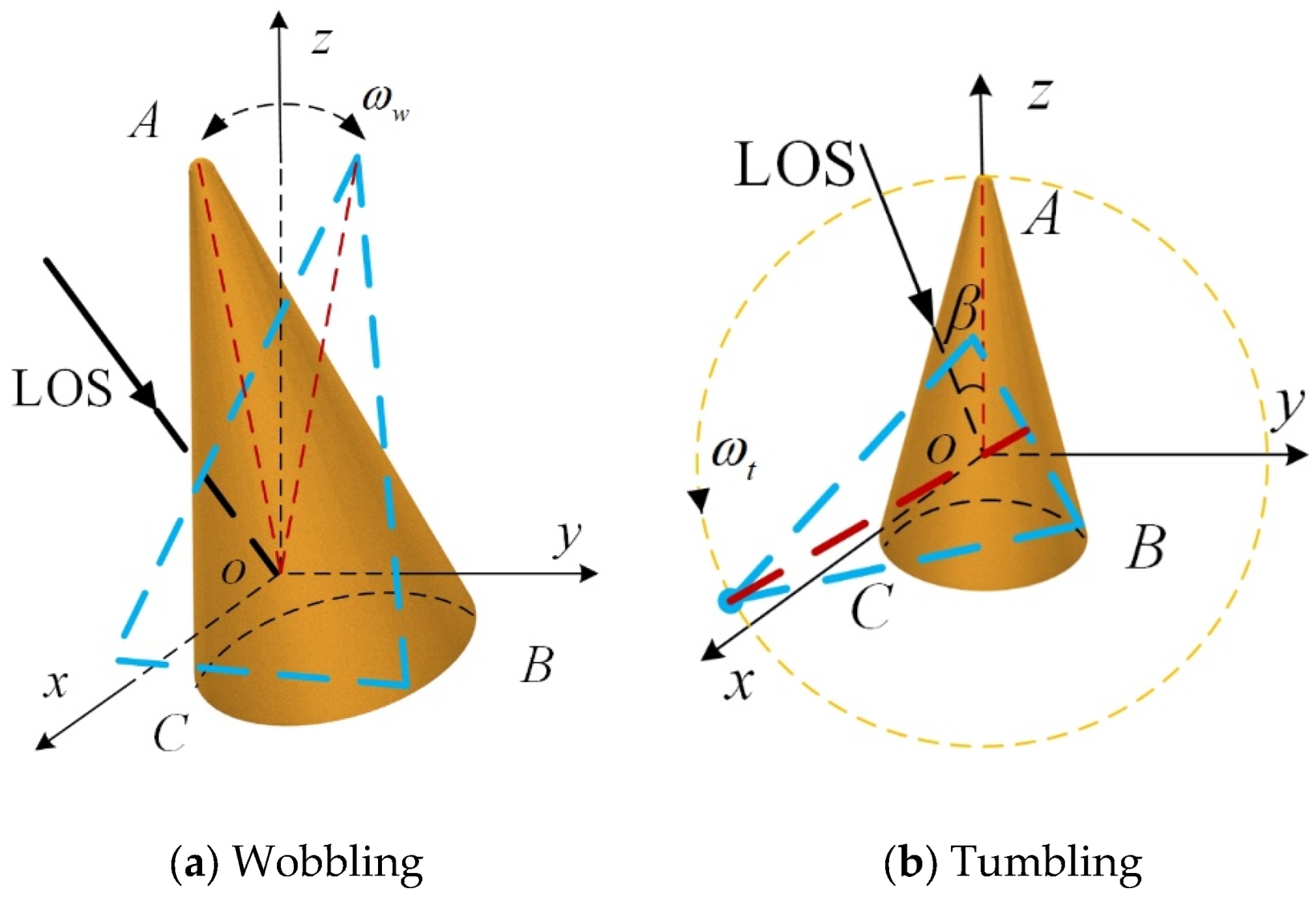
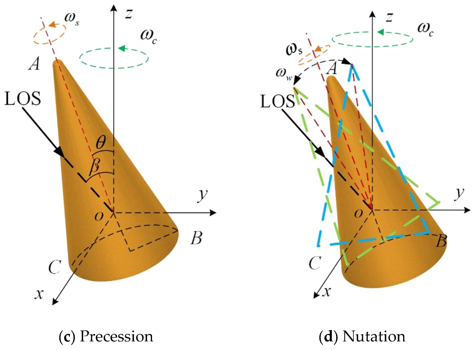
Here, the representative micro-motions for space targets are considered: (1) Wobbling, see Figure 1a. (2) Tumbling, see Figure 1b. (3) Precession, see Figure 1c. and (4) nutation, see Figure 1d [24]. The mass of the cone-shaped space target is set at the origin of the $o-xyz$ coordinate system, the elevation angle of the target symmetry axis is $\theta$, the angle between the radar line-of-sight (LOS) and the $oz$ axis is $\beta$. The initial coning matrix can be expressed as:

$${\mathbf{\Re }}_{Init}=\left[\begin{array}{ccc}1& 0& 0\\ 0& \cos \theta & \sin \theta \\ 0& -\sin \theta & \cos \theta \end{array}\right]$$

(1)

Taking the wobbling motion as an example to analyze, assuming ${\omega }_w$ represents the wobbling angular velocity, the micro-motion matrix at time $t$ is

$${\mathbf{\Re }}_w(t)=I+U_w\sin ({\omega }_{w}t)+U_w{}^2[1-\cos ({\omega }_{w}t)]$$

(2)

where $I$ is the identity matrix and ${\omega }_w$ represents the wobble angular velocity. The skew-symmetric matrix $U_w$ can be defined by

$$U_w=\left[\begin{array}{ccc}0& -{\omega }_{wz}& {\omega }_{wy}\\ {\omega }_{wz}& 0& -{\omega }_{wx}\\ -{\omega }_{wy}& {\omega }_{wx}& 0\end{array}\right]$$

(3)

where ${\omega }_{wx}$, ${\omega }_{wy}$, and ${\omega }_{wz}$ are the projection of ${\omega }_w$ onto the $x$, $y$, and $z-\mathrm{axis}$, respectively.

Then, the micro-range of scattering centers by wobbling are

$$r_w(t)={\mathbf{\Re }}_w(t)·{\mathbf{\Re }}_{init}·{\mathit{r}}_0·\mathit{n}$$

(4)

where $r_0$ is the initial position of scattering centers and $\mathit{n}$ is the unit vector of LOS.

Similarly, at time $t$, the tumbling matrix can be expressed as

$${\mathbf{\Re }}_t(t)=I+U_t\sin ({\omega }_{t}t)+U_t{}^2[1-\cos ({\omega }_{t}t)]$$

(5)

where ${\omega }_t$ represents the tumble angular velocity. $U_t$ represents the skew-symmetric matrix of tumbling angular velocity ${\omega }_t$.

Precession can be considered as the combination of spinning and coning motion, and nutation can be considered as the combination of spinning, coning, and wobbling [25].

Assume ${\mathbf{\Re }}_c$ and ${\mathbf{\Re }}_s$ represent the coning matrix and the spinning matrix, respectively. Then, the precession matrix and nutation matrix can be expressed as

$$\left\{\begin{array}{l}{\mathbf{\Re }}_p(t)={\mathbf{\Re }}_c{\mathbf{\Re }}_s\\ {\mathbf{\Re }}_n(t)={\mathbf{\Re }}_w{\mathbf{\Re }}_c{\mathbf{\Re }}_s\end{array}\right.$$

(6)

Then, the micro-range of scattering centers by tumbling, precession, and nutation are

$$\left\{\begin{array}{l}{r}_t(t)={\mathbf{\Re }}_t(t)·{\mathbf{\Re }}_{init}·{\mathit{r}}_0·\mathit{n}\\ r_p(t)={\mathbf{\Re }}_p(t)·{\mathbf{\Re }}_{init}·{\mathit{r}}_0·\mathit{n}\\ r_n(t)={\mathbf{\Re }}_n(t)·{\mathbf{\Re }}_{init}·{\mathit{r}}_0·\mathit{n}\end{array}\right.$$

(7)

In conclusion, the micro-range characteristics of the wobbling target conform to the law of sinusoidal modulation. If the wobbling angle exceeds $\pi$, the target will rotate in a specific direction around its center of mass, entering the tumbling state. Precession and nutation belong to compound micro-motions which can be regarded as a composite of multiple primary micro-motions. Consequently, the micro-range characteristics of the precession and nutation target will undergo additional modulation on a sinusoidal basis.

Given that the wideband radar emits a linear frequency-modulated (LFM) signal, consequently, the echo signal may be defined as follows

$$s_w(\widehat{t},t_s)={\displaystyle \sum _{k=1}^K{\sigma }_k\mathrm{rect}\left(\frac{\widehat{t}-T_k\left(t_s\right)}{\tau }\right)}·\exp \left(j2\pi \left(f_c\left(t-T_k\left(t_s\right)\right)+\frac{\mu }{2}{\left(\widehat{t}-T_k\left(t_s\right)\right)}^2\right)\right)$$

(8)

where $\widehat{t}$ and $t_s$ represent the fast time and slow time, respectively. $\mu$ is the frequency modulation slope of LFM signal, $f_c$ denotes the wideband radar carrier frequency, $\tau$ is the time duration, and $c$ represents the speed of light. ${\sigma }_k$ and $T_k\left(t_s\right)=2R_k\left(t_s\right)/c$ denote the scattering coefficient and the echo delay time at $t_s$ of the kth scattering center, respectively.

After applying the “dechirp” processing and compensating for the residual video phase, a Fourier transform (FT) is performed on the echo in the fast time domain [26]. Subsequently, $r=c/2\mu f$ is substituted to obtain the expression for the echo in the domain of the time-range, which can be defined as follows:

$$S(r,t_s)={\displaystyle \sum _{k=1}^K{\sigma }_k\tau sinc\left[\frac{2B}{c}\left(r+R_{\Delta k}(t_s)\right)\right]}·\exp \left\{-j\frac{4\pi f_c}{c}{R}_{\Delta k}(t_s)\right\}$$

(9)

where $B$ is the radar bandwidth, and $r$ denotes the motion range. $R_{\Delta k}(t_s)=R_k(t_s)-R_{ref}$; symbol $R_{ref}$ is reference range. $sinc\left(·\right)$ represents the sinc function.

In simulation, the time-range maps can be obtained by Equation (9). Assuming the wideband radar carrier frequency $f_c$ is 10 GHz, the bandwidth $B$ is 2 GHz, and the radar observation time is 2 s. The height and radius of the cone target are 3 m and 0.64 m, respectively.

Figure 2 presents simulation time-range maps of the four micro-motion forms including wobbling, tumbling, precession, and nutation. In wobbling state, the wobble angular velocity $2\pi$ rad/s, the maximum angle of wobbling is $30°$, and the simulation result is shown in Figure 2a. In the tumbling state, the tumble angular velocity ${\omega }_t=1.2\pi$ rad/s, which is the simulation result, as shown in Figure 2b. The cone rotation angular velocity of precession state is $4\pi$ rad/s, and the angle $\beta$ is $12°$. The simulation result of the precession as shown in Figure 2c. For nutation target, the cone rotation angular velocity, wobble angular velocity, $\beta$ and maximum wobbling angle are $4\pi$ rad/s, $2\pi$ rad/s, $12°$ and $20°$, respectively. The simulation result of nutation is shown in Figure 2a.

As shown in Figure 2, the time-range maps of different micro-motion forms have obvious periodicity, but their variation laws are different, which can be used as an important basis for distinguishing different targets.

3. Proposed Framework

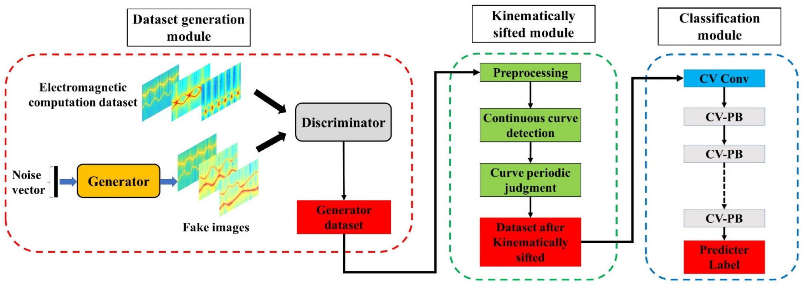
Figure 3 is the schematic diagram of the proposed framework. The basic structure of our proposed framework includes a dataset generation module, a kinematically sifted module, and a classification module. The dataset generation module uses a complex-valued generative adversarial network (CV-GAN) to generator dataset. The module for the kinematic sifted module verifies the compliance of the generated images with the kinematic laws and eliminates any images that violate these laws. The classification module implements target recognition function based on time-range maps. Below are the implementation methods of the three modules.

3.1. Dataset Generation Module

GAN is commonly utilized for various tasks such as generating images, style conversion, and achieving image super-resolution capabilities. Unlike traditional networks, GAN consists of two connected parts, including the generator and the discriminator. The generator is responsible for creating new data samples from random noise. Its role is to generate different but highly similar samples compared to real samples. On the other hand, the discriminator is employed to differentiate between real and generated samples. The generator and the discriminator play a min-max game, and the final optimization goal is to reach Nash equilibrium [27]. The process can be defined as:

$$\underset{G}{\min }\underset{D}{\max }V\left(G,D\right)=E_{y\sim P_{data}}\left[\log \left(D\left(y\right)\right)\right]+E_{z\sim P_z}\left[\log \left(1-D\left(G\left(z\right)\right)\right)\right]$$

(10)

where $y$ is the samples input, and $z$ is the noise vector. $D$ and $G$ defined the generator and the discriminator, respectively. $P_{data}$ and $P_z$ defined the distribution of real data and generated data, respectively.

In the objective function, the discriminator $D$ manages to maximize its ability to distinguish between fake and real images. The generator $G$ aims to minimize the JS divergence between the distribution of generated data and real data.

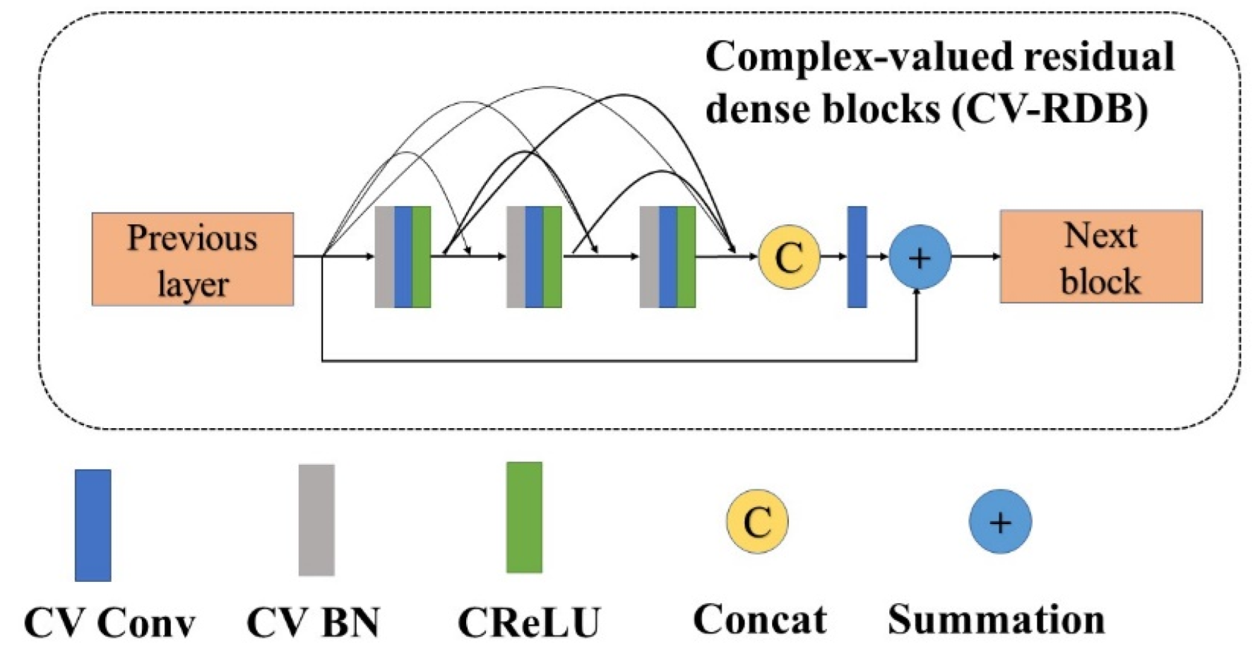
In this paper, this is the first time that the concept of complex values has been used in GAN construction. We use the complex-valued generative adversarial network (CV-GAN) to generate large time-range maps. Similarly, CV-GAN consists of two parts. The generator and discriminator in this paper were composed of complex-valued residual dense blocks (CV-RDB). The structure of CV-RDB is shown in Figure 4.

Figure 4 illustrates the architecture of the CV-RDB, with blue blocks representing the complex-valued convolution layer, gray blocks representing the complex-valued batch normalization (CV BN) layer, green blocks representing the complex-valued activation function, “C” denoting the concatenation operator, and “+” indicating the summation. CV-RDB can be considered as a combination of the residual block and dense block, which can fully extract features and widen the network.

Complex-valued convolution can be defined as

$$M\ast W=\left[\begin{array}{c}\mathbf{\Re }\left(M\ast W\right)\\ \Im \left(M\ast W\right)\end{array}\right]=\left[\begin{array}{cc}{W}_R& -W_I\\ W_I& W_R\end{array}\right]\left(\begin{array}{c}{M}_R\\ M_I\end{array}\right)$$

(11)

where $\mathbf{\Re }\left(·\right)$ and subscript “$R$” represents the real part of complex values, $\Im \left(·\right)$ and subscript “$I$” represents the imaginary part of the complex value. $M=M_R+i{M}_I$ is a complex filter matrix, $W=W_R+i{W}_I$ is a complex vector, and $*$ denotes the convolution operation.

According to Liouville’s theory [28], bounded entire functions must be constants. In a real-valued network, the activation function is often required to be a differentiable function, but in the complex-valued field, a bounded complex activation function cannot be complexly differentiable at the same time. Hence, it is not possible to use the real-valued activation function in a complex-valued network. There is still no agreed consensus on the use of complex-valued activation functions. In this paper, we use complex-valued ReLU (CReLU) [29] as activation function, which can be defined as

$$CReLU\left(z\right)=ReLU\left(\mathbf{\Re }\left(z\right)\right)+iReLU\left(\Im \left(z\right)\right)$$

(12)

where $z\in ℂ$, $ReLU\left(·\right)$ represents the rectified linear unit. ${\theta }_z$ is the phase of $z$. When ${\theta }_z\in \left[0,\frac{\pi }{2}\right]$ or ${\theta }_z\in \left[\pi ,\frac{3\pi }{2}\right]$, real and imaginary parts are either strictly positive or strictly negative at the same time.

Complex-valued networks generally rely upon the CV BN process to accelerate learning. The CV BN can be written as

$$\tilde{x}={\left(C\right)}^{-\frac{1}{2}}\left(x-E\left(x\right)\right)$$

(13)

where $x$ is complex-valued data, $\tilde{x}$ represents normalized complex-valued data, and $C$ is a covariance matrix, which is given by:

$$C=\left(\begin{array}{cc}Cov\left(\mathbf{\Re }\left(x\right),\mathbf{\Re }\left(x\right)\right)& Cov\left(\mathbf{\Re }\left(x\right),\Im \left(x\right)\right)\\ Cov\left(\Im \left(x\right),\mathbf{\Re }\left(x\right)\right)& Cov\left(\Im \left(x\right),\Im \left(x\right)\right)\end{array}\right)$$

(14)

where $Cov\left(\cdot \right)$ represents the covariance operation.

The generator and the discriminator in a dynamic process of continuous confrontation, and finally, CV-GAN can produce many fake images which are sufficiently close to real images. The optimization function of CV-GAN is defined as follows:

$$\begin{array}{ll}\underset{G}{\min }\underset{D}{\max }V\left(D,G\right)& =E_{y\sim P_{data}}\left[\log \left(D\left(\mathbf{\Re }\left(y\right)\right)+D\left(\Im \left(y\right)\right)\right)\right]\\ & +E_{z\sim P_z}\left[\log \left(1-D\left(G\left(\mathbf{\Re }\left(z\right)\right)+G\left(\Im \left(z\right)\right)\right)\right)\right]\end{array}$$

(15)

3.2. Kinematically Sifted Module

It is important to note that the phenomenology of radar data exhibits different properties from optical imagery. In GAN synthetic image conventional evaluation, the visual effect is often regarded as the main evaluation metric. Visual effect evaluation involves assessing the quality of generated images in terms of details, colors, textures, clarity, and other aspects through subjectively judging their visual impact. However, some of the authentic synthetic images may be visually similar, but kinematically impossible. Therefore, using visual effects as the sole evaluation metric for synthetic images may not be accurate.

In this paper, it is necessary to observe the targets continuously over one micro-motion periodic to obtain the periodic and continuous curve images of the targets. We proposed a generation data-sifted method based on physics and kinematics, which can be described as follows:

(1)

Preprocessing: The pixel-wise adaptive Wiener filter [15] was used to preprocess.

(2)

Continuous Curve Detection: Due to the constraints of the radar line of sight, the number of scattering points of cone-shaped targets should not exceed three, which is also reflected in the time-range map, indicating that the number of continuous curves should be no more than three. This paper uses the ShuffleNet [30] to recognize the number of scattering point curves, as shown in Figure 5. The basic unit of the ShuffleNet consists of a group convolution with channel shuffling, as depicted in Figure 5a. Specifically, the original group is divided into multiple subgroups, which are then recombined to form new groups and subsequently undergo group convolution. As illustrated in Figure 5b, the number of groups after channel shuffle is three. The main branch of the basic unit first performs channel-level signal convolution via a 1 × 1 group convolution to the feature map, followed by shuffling the obtained feature map with channel shuffling technology. Subsequently, a 3 × 3 convolution kernel is used to additionally learn the target feature map, and a 1 × 1 group convolution is used to learn the obtained feature map. Moreover, a direct connection structure is adopted in the residual block to guarantee that the quality of the features produced by the next layer of the network does not fall below the quality of the features produced by the previous layer.

To train the network, time-range maps with different numbers of scattering points were generated according to the motion characteristics of different micro-motion targets presented in Section 2. Four labels were constructed to represent images containing one, two, three, and more than three scattering point curves, respectively. The network is trained using the simulation database, and then the generated database is classified to remove images with labels indicating more than three scattering point curves, thus enabling a screening of the number of scattering point curves.

(3)

Curve periodic judgment. We choose $t_i$ as the initial time point. Time-range map sequence $I_i$ at $t_i$ as the reference sequence. Then, we calculate the value of the correlation coefficient between $I_i$ and other sequence $S_i$, which can be described as:

$$sim=\frac{{\displaystyle \sum _i\left(I_i-\overline{I}\right)\left(S_i-\overline{S}\right)}}{\sqrt{\left({\displaystyle \sum _i{\left(I_i-\overline{I}\right)}^2}\right)\left({\displaystyle \sum _i{\left(S_i-\overline{S}\right)}^2}\right)}}$$

(16)

where $\overline{I}$ and $\overline{S}$ denote the average of $I_i$ and $S_i$, respectively.

3.3. Classification Module

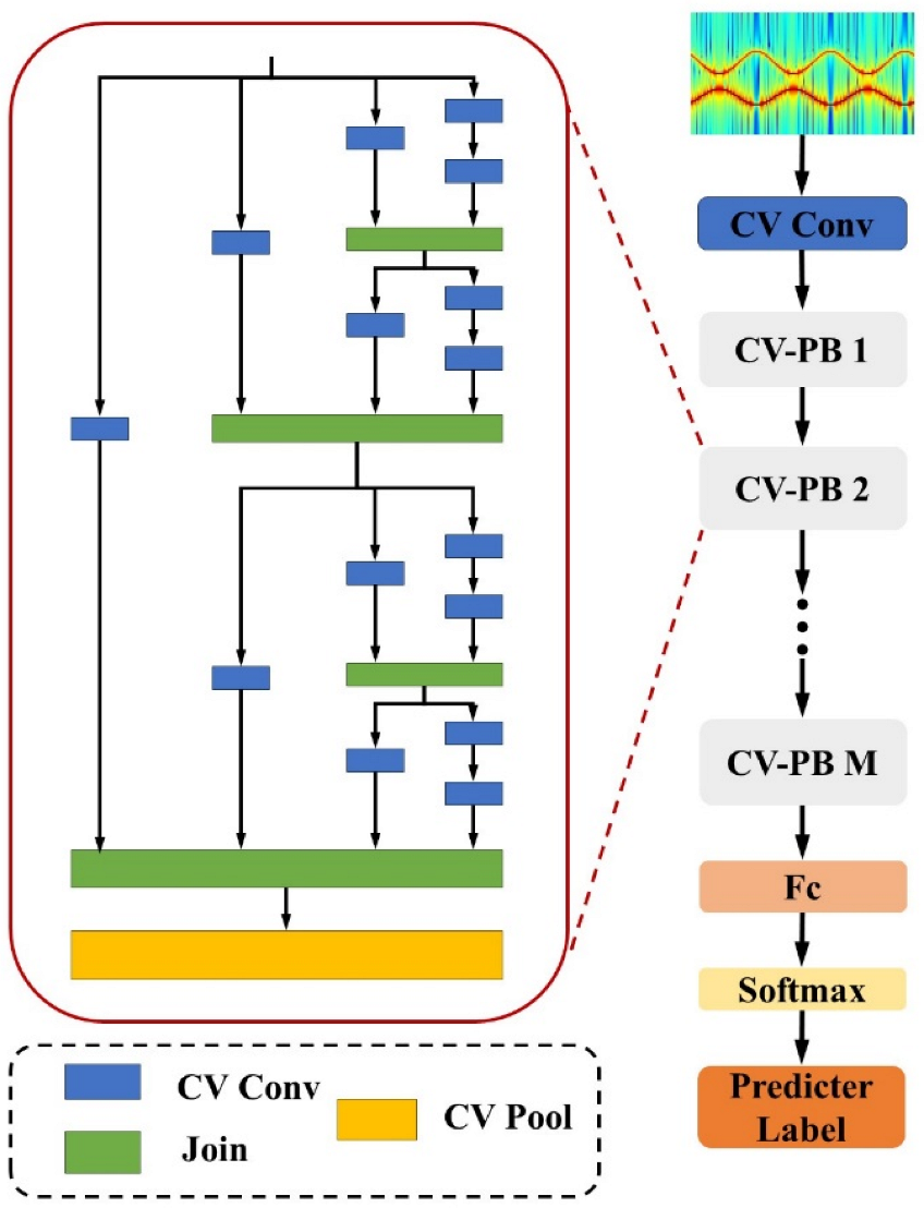
Based on the characteristics of the time-range maps, we use a series of complex-valued parallel block (CV-PB) structures to construct a complex-valued parallel network (CV-PNet). The overall architecture of the CV-PNet is shown in Figure 4.

Assuming the parallel blocks have $N$ parallel branches, the parallel block contains $\left(2^N-1\right)$ convolutional blocks. In Figure 6, where $N=4$, it contains 15 convolutional blocks. Stacking $M$ parallel block and a complex-valued convolution layer yields the parallel network whose total depth, measured in terms of convolution layers, is $M·2^{N-1}+1$.

There are $N$ different types of complex-valued convolutional layers in the parallel block, which are, respectively, $1\times 1$, $3\times 3$, $\cdots$, $\left(2N-1\right)\times \left(2N-1\right)$. In order to reduce computational complexity and expand the network depth, the structural design of parallel blocks follows fractal thinking. First, the $1\times 1$ complex-valued convolutional layer was used as the initial layer. Then, we connect two $1\times 1$ complex-valued convolutional layers in series and combine them with $3\times 3$ complex-valued convolutional layers to obtain the second framework. Then, concatenating two second layer frameworks with $5\times 5$ complex-valued convolutional layers yields the third framework. This continues until two $\left(N-1\right)th$ frameworks are concatenated and then combined with complex-valued $\left(2N-1\right)\times \left(2N-1\right)$ convolutional layers to obtain the $Nth$ framework.

Parallel structures, as opposed to independent convolutional kernels that learn a single feature, have the ability to automatically extract diverse features and demonstrate an increased capacity for handling complex tasks. Different processing branches sample different convolutional kernels, enabling the module to capture features at different scales.

4. Simulation Results and Discussion

4.1. Electromagnetic Computation Dataset

It is technically very hard to obtain real radar echo data of the space cone-shaped target [15,31]. Therefore, to acquire a sufficiently large dataset to drive the synthetic radar image generation with CV-GAN, the electromagnetic computation data was used as the CV-GAN training dataset. The steps for obtaining the CV-GAN training dataset are as follows:

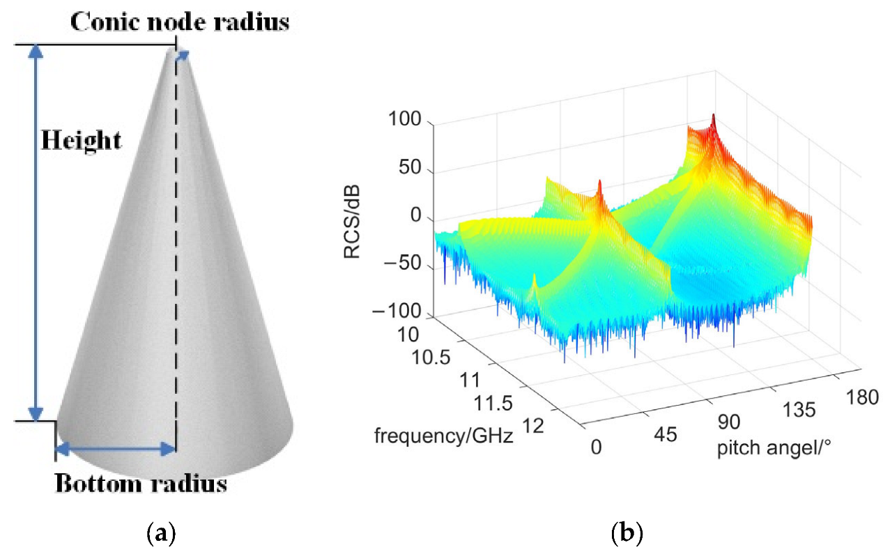
Step 1: Calculation of the radar cross-section (RCS) value for the space target, as shown in Figure 7. Begin by creating a simulation model of the space target. The geometric structure is illustrated in Figure 7a. Next, the simulation model is imported into the FEKO 2019 software, and the Physical Optics (PO) method is applied to calculate the RCS of the target. The parameters used for electromagnetic computation are provided in

Table 3. Parameters of EM Model.

Start frequency	10 GHz	Carrier frequency	12 GHz
End frequency	12 GHz	Polarization	VV
Range of LOS	$0^{\circ }\sim {180}^{\circ }$	Conic node radius	0.075 m
Bottom radius	0.64 m	Height	3 m

. Figure 7b demonstrates the RCS effect.

The RCS value of the target experiences a sudden change at pitch angles of approximately ${79.2}^{\circ }$ and ${180}^{\circ }$. This phenomenon occurs due to the mirror reflection between the generatrix and the base of the cone target, resulting in a significant increase in RCS. Furthermore, due to the occlusion effect, the cone target comprises three scattering centers, and the visibility of these centers is dependent on the pitch angle.

Step 2: Micro-motion parameter setting. According to the RCS of the target, we can obtain the CV-GAN training dataset by setting different target motion parameters, an initial angle, and LOS.

Table 4. Micro-motion parameters of EM computation dataset.

Micro-Motion States	LOS (°)	Angular Velocity (rad/s)	Other Parameters
Wobbling	30:13:147	${\omega }_w$: 0.5$\pi$:0.1$\pi$:1.6$\pi$	Wobbling amplitude (°): 10:3:31
Tumbling	30:5:145	${\omega }_t$: 0.6$\pi$:0.1$\pi$:4.5$\pi$
Precession	30:13:147	${\omega }_c$: 0.9$\pi$:0.1$\pi$:2$\pi$	Precession angle (°): 10:3:31
Nutation	30:13:147	${\omega }_c$: 1$\pi$:0.2$\pi$:2$\pi$${\omega }_w$: 0.4$\pi$:0.2$\pi$:1$\pi$	Wobbling amplitude (°): 10:6:28

presents the settings of the micro-motion parameters.

Step 3: Acquire the echo signal of the space target. Integrate the expressions for the target micro-range under different micro-motions and place the echo expression into the time-range domain in order to generate the time-range maps.

Finally, there are 3840 samples in this EM computation dataset.

4.2. Dataset Generation and Kinematically Sifted Module

The structure of CV-RDB is shown in

Table 5. CV-RDB Architecture.

CV-RDB
CV Conv2d, stride = 1, size = 3 × 3
CV Conv2d, stride = 1, size = 3 × 3
CV Conv2d, stride = 1, size = 3 × 3
Depth Concatenation
CV Conv2d, stride = 1, size = 1 × 1
Addition

. For a simple presentation, the CV BN layer and CReLU layer are not represented.

The network structure of CV-GAN is shown in

Table 6. CV-GAN Architecture.

Generator	Discriminator
Noise, size = 128	Image, size = 128 × 128 × 3
Fully connect	CV Conv2d, stride = 2, filters = 64, size = 3 × 3
CV-RDB, 512	CV-RDB, 128
CV-RDB, 256	CV-RDB, 256
CV-RDB, 128	CV-RDB, 512
CV BN	Fully connect
CV Conv2d, stride = 2, filter s= 64, size = 3 × 3	CReLU
CReLU

.

In this paper, the adaptive moment estimation (Adam) algorithm is employed as the CV-GAN optimizer method, with an exponential decay of 0.5 for the first-order momentum and 0.999 for the second-order momentum. The learning rate is 0.0002. The size of complex-valued convolutional layers in CV-RDB is $3\times 3$, and the step size is 1. The CV BN with the momentum of 0.8.

In this paper, the CV-GAN experiments were implemented using PyCharm, while the kinematically sifted experiments were implemented using MATLAB. The configuration details of the PC platform were as follows: CPU Intel(R) Xeon(R) Gold [email protected] Ghz and RAM 256 GB, and the GPU was an NVIDIA Quadro GV100.

Each training image in CV-GAN is scaled to $128\times 128\times 3$. The minibatch size is 16, and the noise vector of the generator is $128\times 1$ (dimensionality of the latent space). Each time the number of channels in a CV-RDB layer is halved, the length and width are doubled.

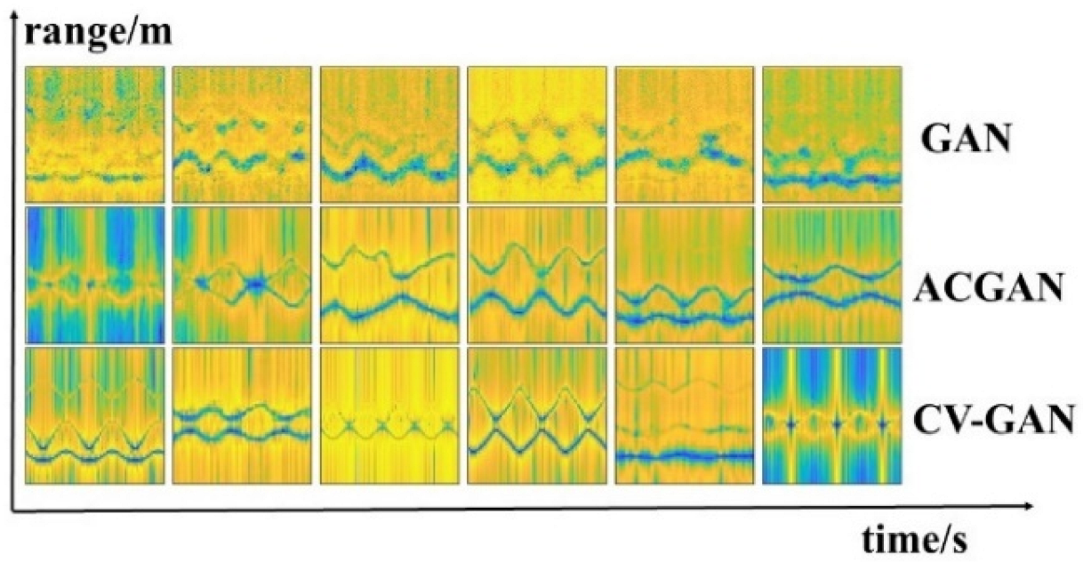
A sample of six time-range maps generated by GAN [19], ACGAN [20], and CV-GAN are depicted in Figure 8. It can be observed that the GAN-generated images appear to be blurry, the ACGAN-generated images are comparatively clear, and the images generated by CV-GAN have the highest imaging quality.

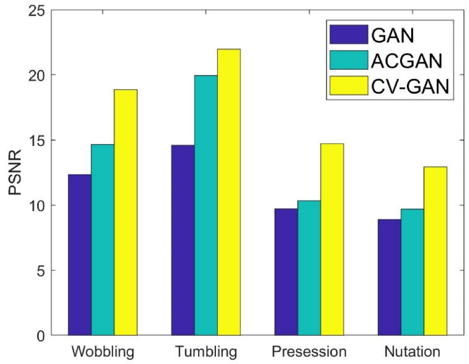
In our evaluation of the quality of generated images, we employed Peak Signal to Noise Ratio (PSNR), an objective evaluation indicator for evaluating noise levels or image distortion that plays a crucial role in ensuring the quality of generated images. PSNR can be defined as:

$$PSNR=10{\log }_{10}\left(\frac{MA{X}_I^2}{MSE}\right)$$

(17)

where $MA{X}_I$ defined the maximum value of image color and $MSE$ is the error of the mean square.

The larger the PSNR, the less distortion and the better the quality of the generated image. In Figure 9, we observe that the images generated using CV-GAN exhibit significantly larger PSNR values, indicating superior image quality compared to other methods.

To quantitatively assess the performance of different methods, Fréchet inception distance (FID) is employed to measure the quality of generated data [32]. FID is mathematically formulated as

$$\mathrm{FID}(P_e,P_s)={‖{\mu }_e-{\mu }_s‖}_2^2+\mathrm{Tr}\left({\sum }_e+{\sum }_s-2{\left({\sum }_e{\sum }_s\right)}^{1/2}\right)$$

(18)

where $P_r$ and $P_s$ denote the distribution of the electromagnetic computation image and synthetic image, respectively. The value of FID is dependent on means ${\mu }_e$, ${\mu }_s$, and covariances ${\sum }_e$, ${\sum }_s$. $\mathrm{Tr}\left(\cdot \right)$ represents the trace of the matrix.

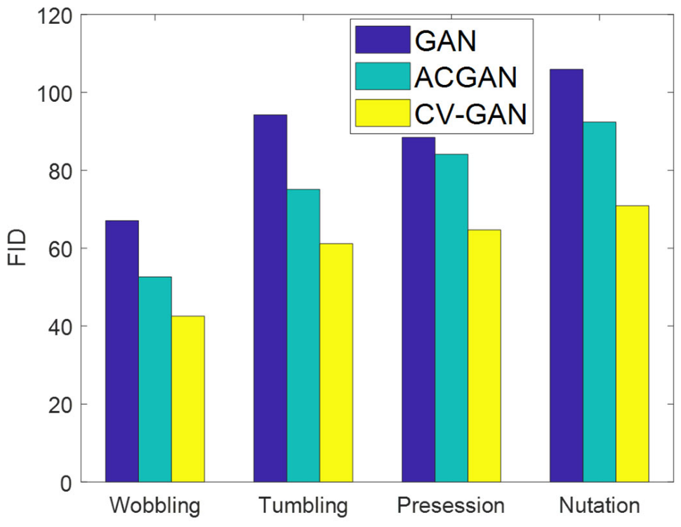
The FID of the time-range maps generated by different methods was calculated. As shown in Figure 10, the generated images based on CV-GAN have a lower FID value, indicating an improved diversity of the images.

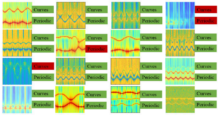
To demonstrate the kinematic sifting method presented in this paper, we randomly selected 16 synthetic images generated by CV-GAN. As illustrated in Figure 11, the green label indicates that the generated image adheres to the motion law, while the red label indicates that the generated image is unsuccessful.

Upon examining this random selection of 16 synthetic images, we discovered that three images did not adhere to the kinematic laws and should be excluded from the generated database. This process was repeated to filter all generated data. As a result, 1273 images of wobbling, 1360 images of tumbling, 1185 images of precession, and 977 images of nutation that did not meet the criteria were eliminated.

4.3. Classification Result

The structure and hyperparameters of the CV-PNet are shown in

Table 7. Classification module architecture and hyperparameters.

CV-PNet	Hyperparameters
Input, size = 128 × 128 × 3	Optimizer: Adam
CV Conv2d, stride = 2, filters = 64, size = 7 × 7	Epochs: 30
Max pooling, stride = 1, size = 5 × 5	Dropout: 0.005
CV-PB (number = 10)	Initial learning rate: 0.001
Global average pooling	Learning rate decay factor: 0.5/5 epoch
Fully connect	Bath size: 12
SoftMax
Output

.

The number of parallel branches is 4 and the size of complex-valued convolutional layers in CV-PB are $1\times 1$, $3\times 3$, $5\times 5$, and $7\times 7$. The step size of all complex-valued convolutional layers is 1.

The performance of the network can be assessed using the classification accuracy, F1 [33], and kappa coefficient [16], which are all values between 0 and 1, with higher values indicating better performance. The definition of the evaluation metric is as follows

$$\mathrm{ACC}=\frac{\mathrm{TP}+\mathrm{TN}}{\mathrm{TP}+\mathrm{TN}+\mathrm{FP}+\mathrm{FN}}$$

(19)

$$\mathrm{MAP}=\frac{1}{Y}{\displaystyle \sum _{i=1}^Y\frac{\mathrm{T}{\mathrm{P}}_i}{\mathrm{T}{\mathrm{P}}_i+\mathrm{F}{\mathrm{P}}_i}}$$

(20)

$$\mathrm{MF}1=\frac{1}{Y}{\displaystyle \sum _{i=1}^Y\frac{2\times \frac{\mathrm{T}{\mathrm{P}}_i}{\mathrm{T}{\mathrm{P}}_i+\mathrm{F}{\mathrm{P}}_i}\times \frac{\mathrm{T}{\mathrm{P}}_i}{\mathrm{T}{\mathrm{P}}_i+\mathrm{F}{\mathrm{N}}_i}}{\frac{\mathrm{T}{\mathrm{P}}_i}{\mathrm{T}{\mathrm{P}}_i+\mathrm{F}{\mathrm{P}}_i}+\frac{\mathrm{T}{\mathrm{P}}_i}{\mathrm{T}{\mathrm{P}}_i+\mathrm{F}{\mathrm{N}}_i}}}$$

(21)

$$\mathrm{KC}=\frac{\mathrm{ACC}-p_e}{1-p_e}$$

(22)

where $Y$ is the number of categories. The abbreviations are as follows: TP (true positive), TN (true negative), FN (false negative), and FP (false positive). $p_e$ is the relative misclassification number. Assuming that the total number of samples is $N$, then

$$p_e=\frac{\left(\mathrm{T}\mathrm{P}+\mathrm{F}\mathrm{N}\right)\times \left(\mathrm{T}\mathrm{P}+\mathrm{F}\mathrm{P}\right)+\left(\mathrm{F}\mathrm{N}+\mathrm{T}\mathrm{N}\right)\left(\mathrm{T}\mathrm{N}+\mathrm{F}\mathrm{P}\right)}{N^2}$$

(23)

We set the electromagnetic computation dataset as Data1, the generated dataset as Data2, and the generated dataset after sifting as Data3. To ensure the preciseness of the experiment, we set the database size of each target micro-motion type in Data2 and Data3 to 8640. The following experiments were designed to verify the effectiveness of the proposed method:

(1)

Experiment 1: We used Data1 as the network training database, with 20% of Data2 allocated as the classification validation database and 20% as the classification testing database.

(2)

Experiment 2: We used Data1 and 60% of Data2 as the classification training database. The settings of the validation database and testing database are kept consistent with Experiment 1.

(3)

Experiment 3: We used Data1 and 60% of Data3 as the classification training database. The settings of the validation database and testing database are kept consistent with Experiment 1.

The test confusion matrixes are depicted in Figure 12.

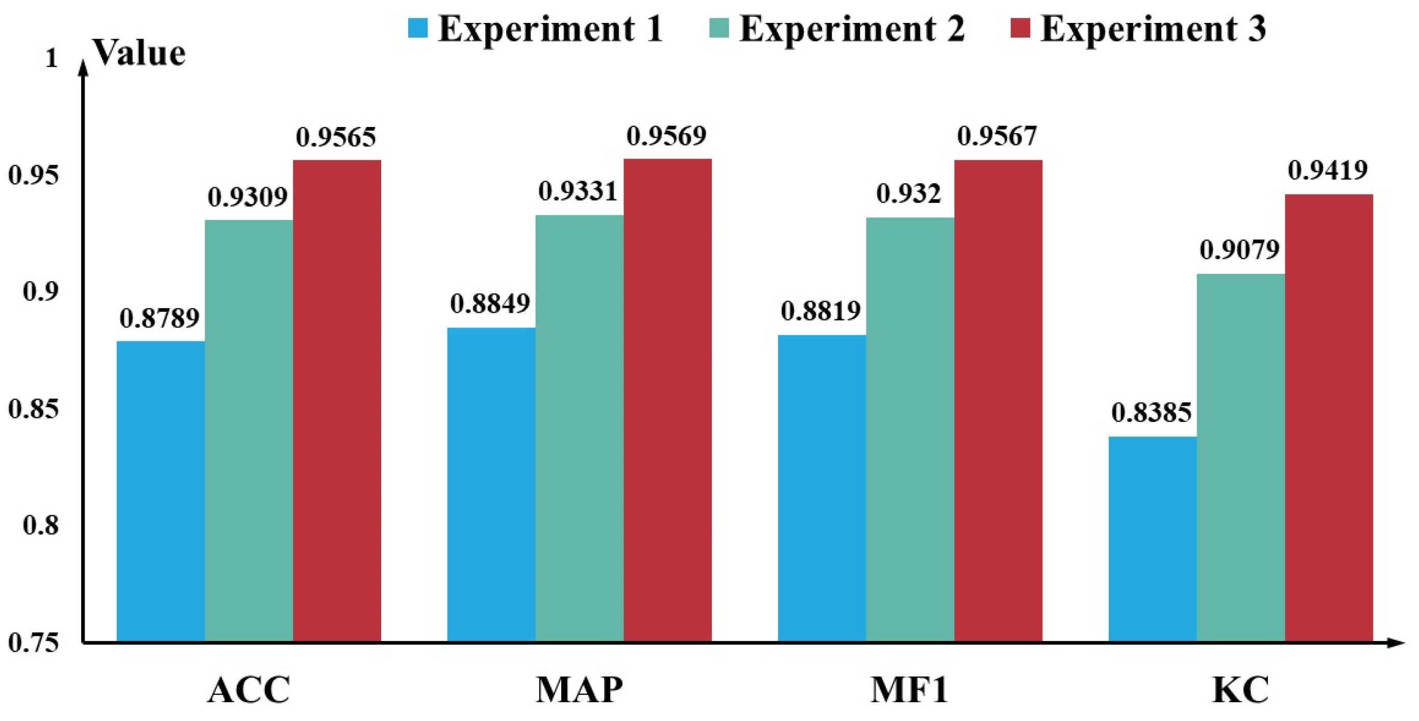
Then, we compute the value of the evaluation metric based on the confusion matrix. The confusion matrix of experiment 1, experiment 2 and experiment 3 is shown in Figure 12a–c. Figure 13 illustrates that the four indicators of the experiment 3 are the best and the experiment 2 is slightly inferior, whereas experiment 1 is poor. The worst recognition performance of experiment 1 was attributed to the small number of samples in the electromagnetic dataset, while the best performance accuracy of experiment 3 verified the importance of kinematically sifted experiments.

To further verify the effectiveness of the method, we compared the proposed networks with the following state-of-the-art target recognition algorithms. (1) TARAN [14]; (2) 2D CNN [15]; (3) 19-layer CNN [19].

Table 8. Performance comparison with different networks.

	ACC	MAP	MF1	KC
TARAN [14]	0.9447	0.9451	0.9449	0.9263
2D CNN [15]	0.9284	0.9292	0.9288	0.9045
19-layer CNN [19]	0.9179	0.9178	0.9179	0.8906
CV-PNet	0.9565	0.9569	0.9567	0.9419

shows that under the same dataset, the proposed networks achieve a better performance in terms of ACC, MAP, MF1, and KC.

Then, based on the initial network structure, we studied the influence of the number of parallel blocks (M) and the number of parallel branches (N) in the proposed CV-PNet. The Data3 dataset for each class was randomly divided into 60% for training, 20% for validation, and 20% for testing. The comparison results are illustrated in

Table 9. Effects of parallel block.

	ACC	MAP	MF1	KC
$M=4$	0.8411	0.8467	0.8439	0.7882
$M=6$	0.8919	0.8925	0.8922	0.8559
$M=8$	0.9362	0.9367	0.9364	0.9149
$M=10$	0.9565	0.9569	0.9567	0.9419
$M=12$	0.9648	0.9658	0.9653	0.9531

and

Table 10. Effects of parallel branches.

	ACC	MAP	MF1	KC
$N=2$	0.7878	0.7882	0.7880	0.7170
$N=3$	0.8659	0.8819	0.8738	0.8212
$N=4$	0.9565	0.9569	0.9567	0.9419
$N=5$	0.9635	0.9649	0.9642	0.9514

.

As shown in Table 9, the number of parallel blocks (M) is increased from 4 to 12 in an interval of 2. As the value of M increased, the evaluation metric values gradually increased. It is noteworthy that the recognition effect of CV-PNet significantly improved when M was between 4 and 10. However, beyond M = 10, the recognition effect showed a slower improvement. One can observe from Table 10 that as the number of parallel branches increases, so does the recognition ability of CV-PNet.

5. Conclusions

This research introduces a comprehensive framework for classifying space micro-motion targets. The framework is composed of three key modules: a dataset generation module that utilizes CV-GAN to produce high-quality time-range maps, a kinematically sifted module that ensures compliance with kinematics laws, and a classification module designed to accurately recognize space micro-motion targets. Experimental results have unequivocally demonstrated the effectiveness of this proposed framework.

In future studies, we plan to expand the database generation method to include the time-frequency domain and range-doppler domain. Additionally, we will explore the impact of various radar images on the classification performance, aiming to further enhance the classification accuracy. These advancements will contribute to a more versatile and reliable classification framework for space micro-motion targets.