Article

Assessment of Combined Reflectance, Transmittance, and Absorbance Hyperspectral Sensors for Prediction of Chlorophyll a Fluorescence Parameters

by
Renan Falcioni
1,*,
Werner Camargos Antunes
1,
Roney Berti de Oliveira
1,
Marcelo Luiz Chicati
1,
José Alexandre M. Demattê
2 and
Marcos Rafael Nanni
1
1
Department of Agronomy, State University of Maringá, Av. Colombo, 5790, Maringá 87020-900, Paraná, Brazil
2
Department of Soil Science, Luiz de Queiroz College of Agriculture, University of São Paulo, Av. Pádua Dias, 11, Piracicaba 13418-260, São Paulo, Brazil
*
Author to whom correspondence should be addressed.
Remote Sens. 2023, 15(20), 5067; https://doi.org/10.3390/rs15205067
Submission received: 15 September 2023 / Revised: 12 October 2023 / Accepted: 21 October 2023 / Published: 22 October 2023

Abstract

:
Photosynthesis is a key process in plant physiology. Understanding its mechanisms is crucial for optimizing crop yields and for environmental monitoring across a diverse range of plants. In this study, we employed reflectance, transmittance, and absorbance hyperspectral sensors and utilized multivariate statistical techniques to improve the predictive models for chlorophyll a fluorescence (ChlF) parameters in Hibiscus and Geranium model plants. Our objective was to identify spectral bands within hyperspectral data that correlate with ChlF indicators using high-resolution data spanning the electromagnetic spectrum from ultraviolet to shortwave infrared (UV–VIS–NIR–SWIR). Utilizing the hyperspectral vegetation indices (HVIs) tool to align importance projection for wavelength preselection and select the most responsive wavelength by variable importance projection (VIP), we optimized partial least squares regression (PLSR) models to enhance predictive accuracy. Our findings revealed a strong relationship between hyperspectral sensor data and ChlF parameters. Employing principal component analysis, kappa coefficients (k), and accuracy (Acc) evaluations, we achieved values exceeding 86% of the predicted ChlF parameters for both Hibiscus and Geranium plants. Regression models for parameters such as Ψ(EO), ϕ(PO), ϕ(EO), ϕ(DO), δRo, ρRo, Kn, Kp, SFI(abs), PI(abs), and D.F. demonstrated model accuracies close to 0.84 for R2 and approximately 1.96 for RPD. The spectral regions linked with these parameters included blue, green, red, infrared, SWIR1, and SWIR2, emphasizing their relevance for noninvasive evaluations. This research demonstrates the ability of hyperspectral sensors to noninvasively predict chlorophyll a fluorescence (ChlF) parameters, which are essential for assessing photosynthetic efficiency in plants. Notably, hyperspectral absorbance data were more accurate in predicting JIP-test-based chlorophyll a kinetic parameters. In conclusion, this study underscores the potential of hyperspectral sensors for deepening our understanding of plant photosynthesis and monitoring plant health.

1. Introduction

Light plays a fundamental role in plant physiological processes, most notably in photosynthesis [1]. The way plants perceive and utilize light triggers a cascade of biochemical and physiological responses [2]. Chlorophyll a fluorescence (ChlF) is a primary indicator of photosynthetic efficiency, shedding light on the electron transport rate, photochemical quenching, and nonphotochemical quenching within photosystem II (PSII) [3]. Traditionally, pulse-amplitude-modulation (PAM) fluorometry, which employs the saturation pulse method, has been the go-to technique for ChlF quantification [4]. Parameters such as Fv/Fm and Fv’/Fm’ are instrumental in evaluating the health and efficiency of the photosynthetic machinery [5].
However, the demand for expansive, noninvasive, and real-time methodologies to assess the photosynthetic apparatus has increased, leading to the application of hyperspectral remote sensing [6]. Hyperspectral sensors, which record reflectance data spanning the visible to shortwave infrared spectra, provide in-depth insights into plant biochemical and biophysical properties [7]. Each hyperspectral band is associated with distinct molecular interactions, including vibrational bands and stretching, which are indicative of specific compounds such as pigments (flavonoids, anthocyanins, chlorophylls, xanthophyll, and carotenes) and structures such as lignin, cellulose, and hemicellulose, as well as water bands. These associations provide insight into the physiological and morphological characteristics of a range of plants. In addition, the hyperspectral band corresponds to specific molecular interactions and sheds light on various physiological and morphological attributes of plants. Additionally, these bands are proposed to correlate with the photosynthetic components of leaves, such as proteins, carbohydrates, structural lipids, and energy organelles, such as mitochondria and chloroplasts [8,9,10].
Hyperspectral analysis, which involves interpreting data from these sensors, captures information across numerous contiguous electromagnetic spectrum bands, setting it apart from multispectral sensors [11,12,13]. The detailed nature of hyperspectral sensors allows for the identification of minor spectral variations, facilitating material differentiation and the detection of specific properties. This analysis has been invaluable in sectors such as agriculture, plant monitoring, environmental monitoring, and assessing photosynthetic parameters [14,15,16].
The JIP-test, a standard in ChlF analysis, extracts parameters from ChlF emission kinetics and delineates energy transitions from PSII to PSI [13,17,18]. Integration of high-resolution hyperspectral data can enhance JIP-test predictions and expand its applicability. However, this integration necessitates rigorous calibration, validation, and the application of appropriate statistical methods. In this sense, the JIP-test offers insights into chlorophyll a fluorescence transients, shedding light on plant photosynthetic efficiency and health [19,20]. From this test, several key parameters emerge. For example, Ψ(EO) measures how effectively a trapped exciton can move an electron beyond QA in the electron transport chain. Ψ(RO) gauges the transfer efficiency of an electron from the intersystem carriers to the PSI end electron acceptors. ϕ(PO) represents the primary photochemistry’s maximum quantum yield, while ϕ(EO) and ϕ(RO) provide quantum yields for electron transport from QA to the PSI end electron acceptors and their reduction, respectively. ϕ(DO) indicates the quantum yield of nonphotochemical energy dissipation due to donor-side limitations. δRo relates to the movement efficiency of an electron from reduced intersystem carriers to the PSI end electron acceptors. ρRo shows how efficiently a reduced PSI end electron acceptor is oxidized. Kn and Kp are nonphotochemical and photochemical quenching coefficients, respectively. SFI(abs) denotes specific flux per absorption, PI(abs) is a performance index based on absorption, and D.F. stands for driving force. Together, these parameters provide a comprehensive understanding of photosynthesis, helping to assess the health and efficiency of the photosynthetic apparatus [21,22,23,24].
Multivariate analyses such as partial least squares (PLS) and principal component analysis (PCA) have been employed for hyperspectral data interpretation [13,25]. These methods facilitate dimensionality reduction, revealing patterns and aiding in predictive model formulation. Within this framework, the selection of the wavelength is critical to maximizing information-based interaction, contributing to optimized component efficiency. The hyperspectral vegetation indices (HVI) tool is instrumental in this process because it identifies more relevant spectral bands. Utilizing HVI for wavelength preselection optimizes PLS model efficacy, ensuring enhanced prediction accuracy [13,15,26,27].
Therefore, this research aims to exploit the capabilities of hyperspectral sensors in capturing data essential for predicting chlorophyll a fluorescence parameters. The objective of this study was to identify the spectral bands within hyperspectral data that correlate with chlorophyll a fluorescence indicators. The research also emphasizes the integration and optimization of advanced reflectance, transmittance, and absorbance hyperspectral sensors to capture all leaf information and apply multivariate statistical methods, including PCA and PLS, to enhance the predictive accuracy of hyperspectral datasets for chlorophyll a fluorescence, as shown in Figure 1.

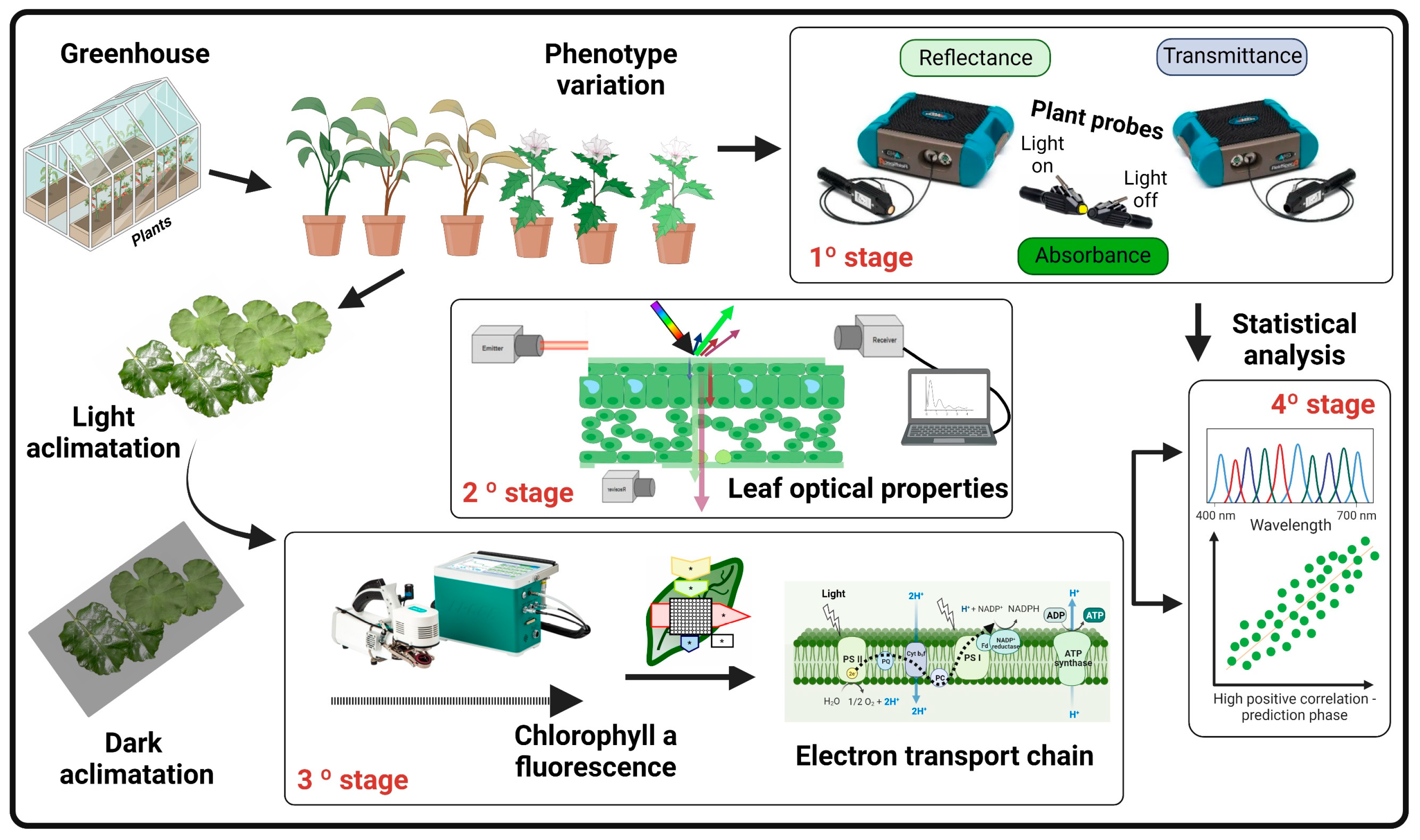
2. Materials and Methods

2.1. Plant Material and Experimental Design

Hibiscus rosa-sinensis L. (Hibiscus) and Pelargonium zonale L’Hér. Ex. Aiton (Geranium) plants were cultivated in 2 L pots in the Botanical Garden at the State University of Maringá, Brazil, under greenhouse conditions. These conditions provided natural ambient light, with temperatures maintained between 22 °C and 26 °C and a photoperiod of 16 h. To ensure consistent hydration, the plants were watered twice daily, specifically at 8 a.m. and 6 p.m. For the study, leaves of various ages and different positions (apex, middle, and base) were sampled from different parts of the plants. A total of 200 samples were collected for both hyperspectral reflectance analysis and assessment of leaf biochemical profiles. To guarantee uniformity in data collection, all measurements were conducted between 11 a.m. and 1 p.m. A summarized scheme of the flowchart analyses can be observed in Figure 1.

2.2. OJIP Chlorophyll a Fluorescence Transient

Measurements on leaves were conducted using an infrared gas exchange analyzer (IRGA; LI-6800, LI-COR Inc., Lincoln, NE, USA) equipped with a Multiphase FlashTM Fluorometer (LI-6800-01; LI-COR Inc., Lincoln, NE, USA). The settings maintained were as follows: a constant 400 µmol mol−1 in the chamber sample (CO2_sample), 60% sample chamber relative humidity (%RH_sample), a flow rate of 700 µmol s−1, a fan speed of 10,000 rpm, and a 25 °C heat exchanger temperature for the sample (Theat_sample) within a 6 cm2 sample chamber. The sensor employed operates at >720 nm, specifically for chlorophyll fluorescence [6].
The induction of chlorophyll a fluorescence transients was carried out using an LI-6800 instrument on the same leaves used for the reflectance, transmittance, and absorbance hyperspectral measurements. Prior to measurement, each chosen leaf underwent dark acclimation overnight for 12 h. Subsequently, a clipping chamber was used, and a saturating light pulse of 15,000 µmol m−2 s−1 was applied for 1 s in induction mode, ensuring the closure of all reaction centers. The methodology for data analysis and the equations for calculating JIP-test parameters have been detailed in previous studies [6,13]. The Biolyzer software version 4.0® (Laboratory of Bioenergetics, University of Geneva; Geneva, Switzerland) facilitated the estimation of JIP-test parameters linked to the electron transport chain in plants [13].

2.3. Hyperspectral Optical Leaf Properties

Leaf reflectance (R) and transmittance (T) were measured using a FieldSpec® 3 Spectroradiometer (Analytical Spectral Devices ASD Inc., Longmont, CO, USA) equipped with an ASD Contact PlantProbe® with a 10 mm diameter [1]. This device incorporates 512 Si photodiodes, capturing wavelengths between 350–2500 nm. To reduce atmospheric interference, a PlantProbe® leaf clip (Analytical Spectral Devices ASD Inc., Boulder, CO, USA) was employed. The data were preprocessed to switch the sensor at 1000 and 1800 nm using the ViewSpec Pro software version 6.2 (ASD Inc., Boulder, CO, USA). Calibration and optimization of the equipment were achieved using standard white reference plates (Spectralon®, Labsphere Inc., Longmont, CO, USA) as per [1]. The plant probe directed a high-intensity light beam onto the leaf’s upper surface, whereas another probe, with its light beam deactivated, assessed the leaf’s lower surface. Both reflectance and transmittance for each wavelength were recorded concurrently. Absorbance was determined using the formula [A = 1 − (R + T)] [1,13].

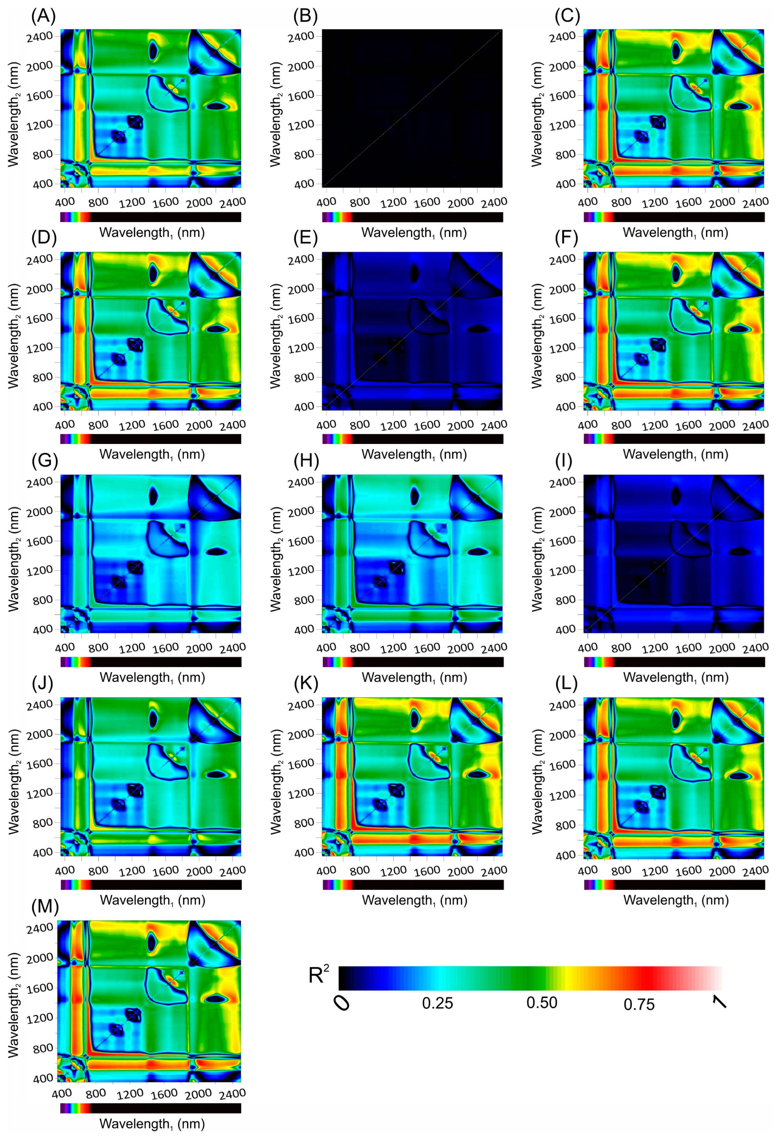
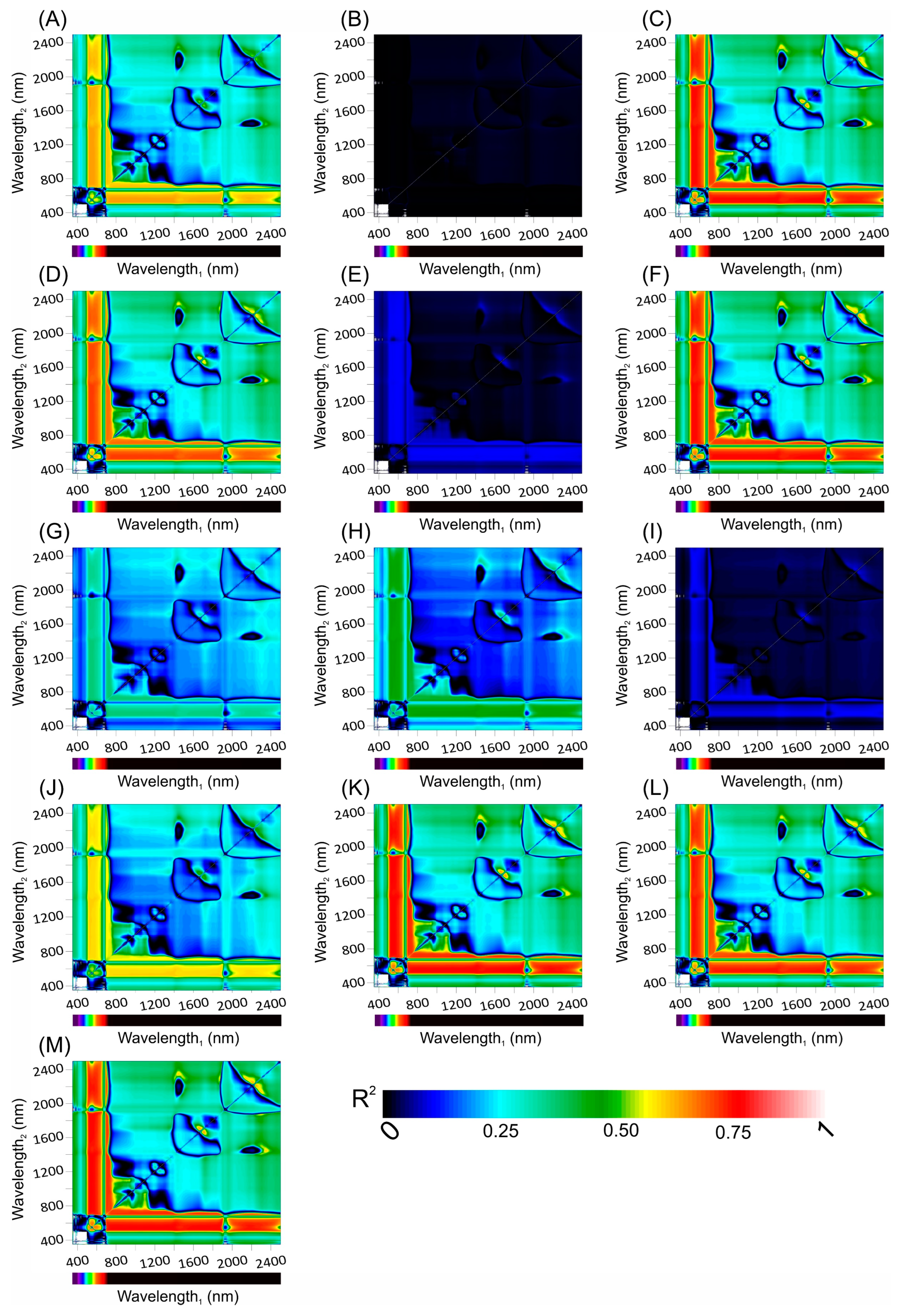
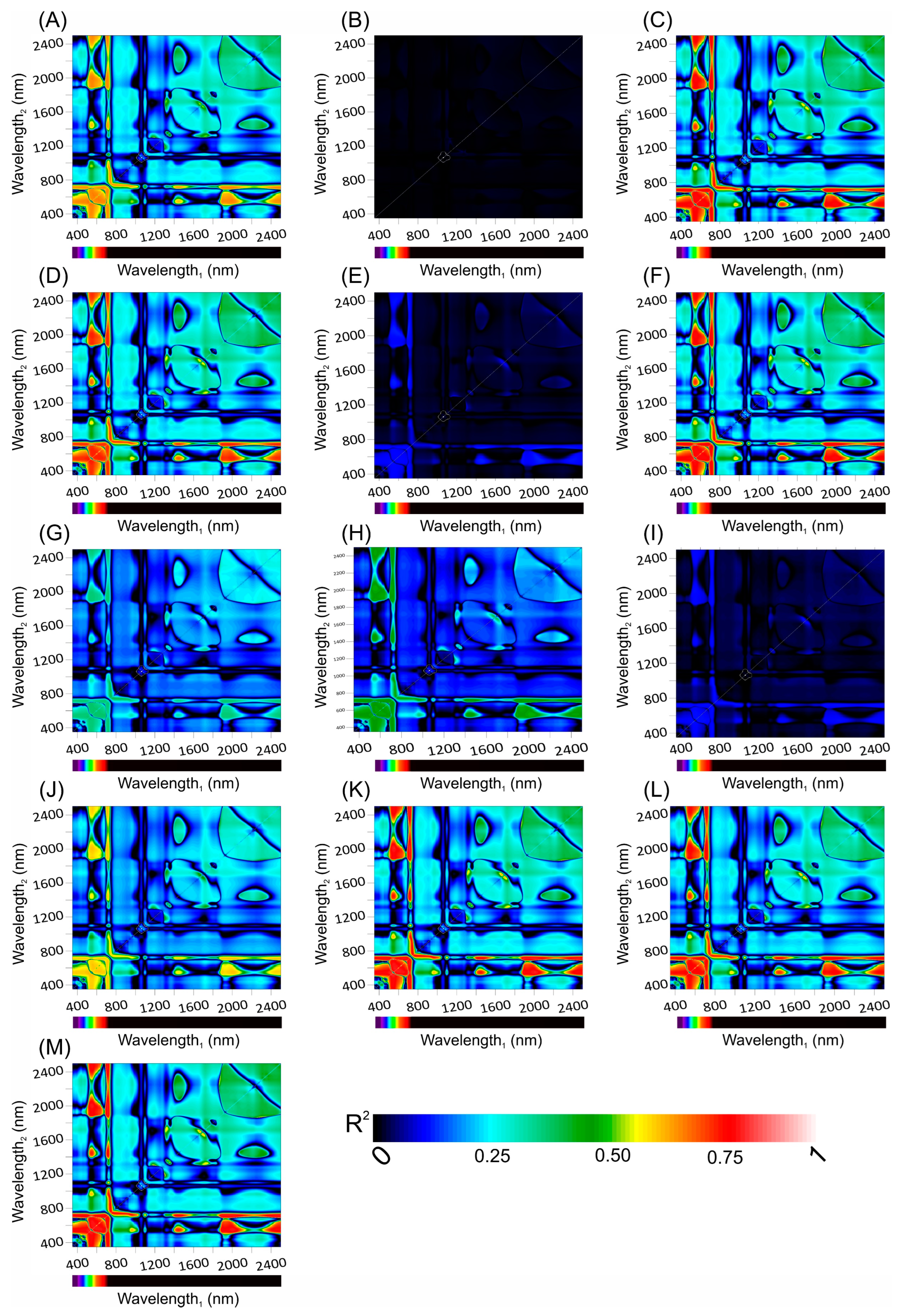
2.4. Analysis of Leaf Spectral Fingerprints

The hyperspectral curves, parameters derived from the hyperspectral data, and JIP-test parameters were used for decision analysis. The effect of the Hibiscus and Geranium plants on the leaf traits was analyzed by one-way analysis of variance (ANOVA). The effects of variety on the reflectance (R), transmittance (T), and absorbance (A) profiles were assessed using PERMANOVA and variable importance projections (VIPs) exactly as described in [6].

2.5. Hyperspectral Vegetation Indices Using Optimal Wavelengths for JIP-Test Parameters

To optimize the accuracy of JIP-test parameter assessments, key hyperspectral bands were identified using the normalized difference vegetation index formula (Equation (1)) drawn from Crusiol et al. (2023) [28]. This approach generated distinct hyperspectral vegetation indices (HVIs). Each HVI was correlated with cross-sections relevant to chlorophyll a kinetic parameters. Correlations were quantified via the Pearson correlation coefficient and the coefficient of determination (R2) using a custom IDL code. A ground-based sensor captured spectra from 350 nm to 2500 nm, with results depicted in a contour map.
H V I = W a v e l e n g t h   1 W a v e l e n g t h   2 W a v e l e n g t h   1 + W a v e l e n g t h   2

2.6. Partial Least Squares Regression (PLSR) by Analysis of Spectroscopy Data

Hyperspectral data were centered on the mean and subjected to PLSR. To obtain prediction models of JIP-test parameters, the spectral data of the different parameters of 200 samples were divided into two groups: 75% (150) of the samples in the first group, with the aim of creating the model (training), and the remaining 25% (50) in the second group, with the aim of testing (prediction) to adjust the model, as described in [13,29]. This proportion (75:25) was selected to ensure estimates that were (1) valid, in the sense that they did not overestimate the accuracy (i.e., did not underestimate the approximation error), and (2) the most accurate among all valid estimates (i.e., their overestimation of the approximation error was the smallest possible), based on a previous analysis described in [13,25,29].
Calibration (Cal) and cross-validation (Cva) were used to predict the quality attributes based on the JIP-test. In addition, the predictive ability of the calibration model was evaluated by calculating metrics such as the coefficient of determination (R2; 1 − S S r e s S S t o t ), offset, root mean square error (RMSE; i = 1 n ( Ŷ i Y i ) 2 n ), and ratio of performance to deviation (RPD; 1 1 R x 2 ), and bias was used to assess the quality, precision, and accuracy of the model, as described in [6].

2.7. Statistical Analyses

2.7.1. Descriptive, Univariate, and Multivariate Statistical Analyses

To characterize the JIP-test metrics, descriptive statistics were employed. For each parameter, evaluations included the count (n), mean, median, minimum, maximum, and coefficient of variation (CV, %), as delineated by [6]. The categorization of CV was observed according to the criteria proposed by Zar (2010) [30]. To ascertain the interrelationships between the biophysical attributes, Pearson’s correlation methodology was harnessed. For these analytical tasks, we used Statistica 10® (StatSoft Inc., Tulsa, OK, USA) and the R software framework. Graphical depictions were generated using a suite of applications: SigmaPlot 10.0® (Systat Inc., Santa Clara, Silicon Valley, CA, USA), R packages, Excel (Microsoft Inc., Silicon Valley, CA, USA), and CorelDraw 2020® (Corel Corp., Ottawa, ON, Canada).

2.7.2. Principal Component Analysis (PCA)

The Unscrambler X software, version 10.4 (CAMO Software, Oslo, Norway), was used to conduct PCA on the growth parameter data, with a statistical significance level set at p < 0.01. To avoid underfitting and overfitting, the optimal number of principal components was determined based on the first maximum value of overall accuracy [31].

3. Results

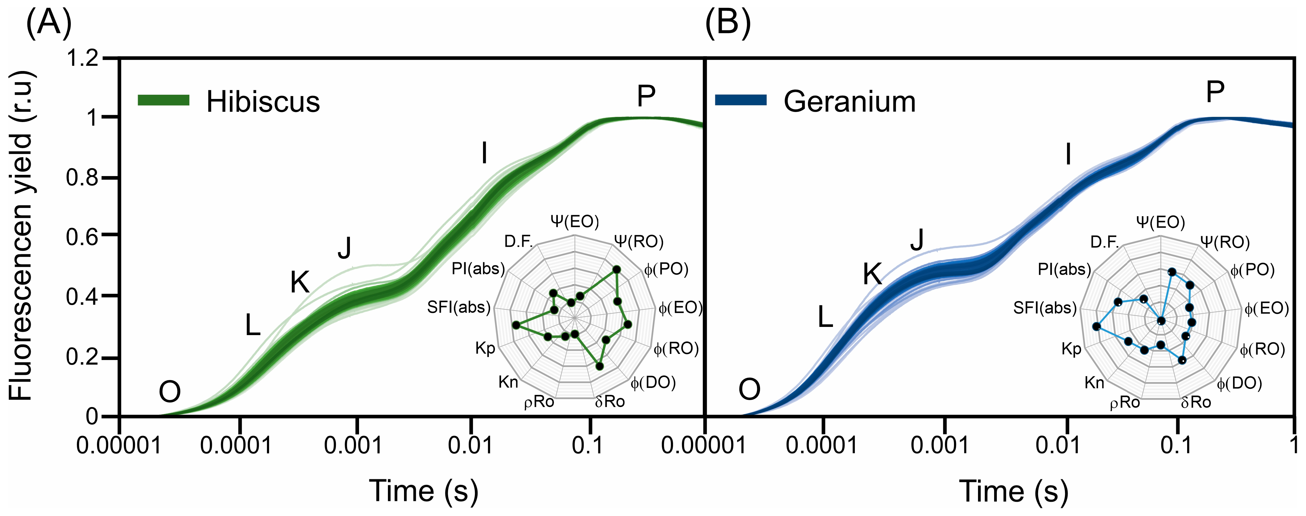
3.1. Description Statistical for Chlorophyll a Fluorescence

Table 1 shows the chlorophyll a parameters in Hibiscus and Geranium, with 200 samples analyzed for each parameter. For Ψ(EO), the mean was 0.57, with a median of 0.57, spanning a minimum of 0.46 to a maximum of 0.64, and a coefficient of variation of 6.1%. Ψ(RO) showed a mean of 0.17, a median of 0.17, a range of 0.14 to 0.22, and a variation coefficient of 7.2%. The ϕ(PO) parameter had a mean of 0.76, a median of 0.76, and values between 0.71 and 0.82, with a 3.5% coefficient of variation. For ϕ(EO), the mean was 0.43, the median was 0.42, with values from 0.33 to 0.51, and the variation was 9.4%. The ϕ(RO) had a mean and median of 0.13, values from 0.11 to 0.18, and a coefficient of variation of 8.1%. For the ϕ(DO) parameter, the mean was 0.24, the median was 0.24, and it ranged from 0.18 to 0.28 with an 11.2% variation. δRo had a mean of 0.31, a median of 0.31, and values between 0.25 and 0.45, with a 9.1% coefficient of variation. ρRo exhibited a mean of 0.74, a median of 0.73, values from 0.53 to 1.12, and a variability of 13.9%. The mean and median of Kn were both 0.005, with a range of 0.005 to 0.006 and a 5.6% variation. Kp had a mean of 0.017 and a median of 0.016, with values stretching from 0.013 to 0.021 and a 10.5% coefficient of variation, respectively. The SFI(abs) parameter had a mean of 1.31, a median of 1.23, ranged from 0.78 to 1.87, and exhibited a variation of 24.2%. PI(abs) indicated a mean of 13.76, a median of 11.61, values from 5.03 to 26.44, and a pronounced variation of 41.8%. Last, for the D.F., the mean was 2.53, the median was 2.45, the range was between 1.62 and 3.28, and the coefficient of variation was 17.1% (Table 1).

3.2. Chlorophyll a Fluorescence Kinetics

Photosynthetic performance was evaluated using OJIP curves and variable fluorescence curves (Figure 2). These analyses revealed a significant pigment variation between Hibiscus (Figure 2A) and Geranium (Figure 2B) (p < 0.01). Declines in ΔVt were observed at ΔL (~20 µs), ΔK (~300 µs), ΔJ (~2 ms), ΔI (~10 ms), and ΔP (~40 ms) (Figure 2A,B). Distinct patterns were identified in the chlorophyll a fluorescence curves of Hibiscus and Geranium. Data points O, L, K, J, I, and P demonstrated significant variations between the two species (Figure 2). Notably, while points O and P exhibited nearly identical fluorescence intensities for both species, Geranium consistently displayed elevated values at the L, K, J, and I points compared to Hibiscus (Figure 2).
ΔVt kinetics suggested a decreased efficiency in the light-harvesting complex, active RCs, and electron transport between PSII and PSI, as depicted in Figure 2. These findings align with the JIP-test parameters. The JIP-test indicated that the Ψ(EO) value for Hibiscus was 0.6017, 11.3% higher than Geranium’s value of 0.5407. Other metrics, such as Ψ(RO) and ϕ(PO), follow a similar trend. However, Geranium outperformed in the ϕ(DO) and δRo parameters. For ρRo, Hibiscus demonstrated superior values, but Geranium was higher in the Kn and Kp metrics. Geranium’s SFI(abs) value of 0.5079 was 37.1% higher than that of Hibiscus at 0.3705. The PI(abs) values were more closely matched, with Geranium’s value of 0.5132 being 10.2% higher than Hibiscus’ value of 0.4657. For the D.F. metric, Geranium’s value of 0.4166 exceeded Hibiscus’s value of 0.3706 by 12.4%. Therefore, the combined analysis of fluorescence data and JIP-test parameters provides insights into the photosynthetic differences between Hibiscus and Geranium plants (Figure 2A,B; insets).

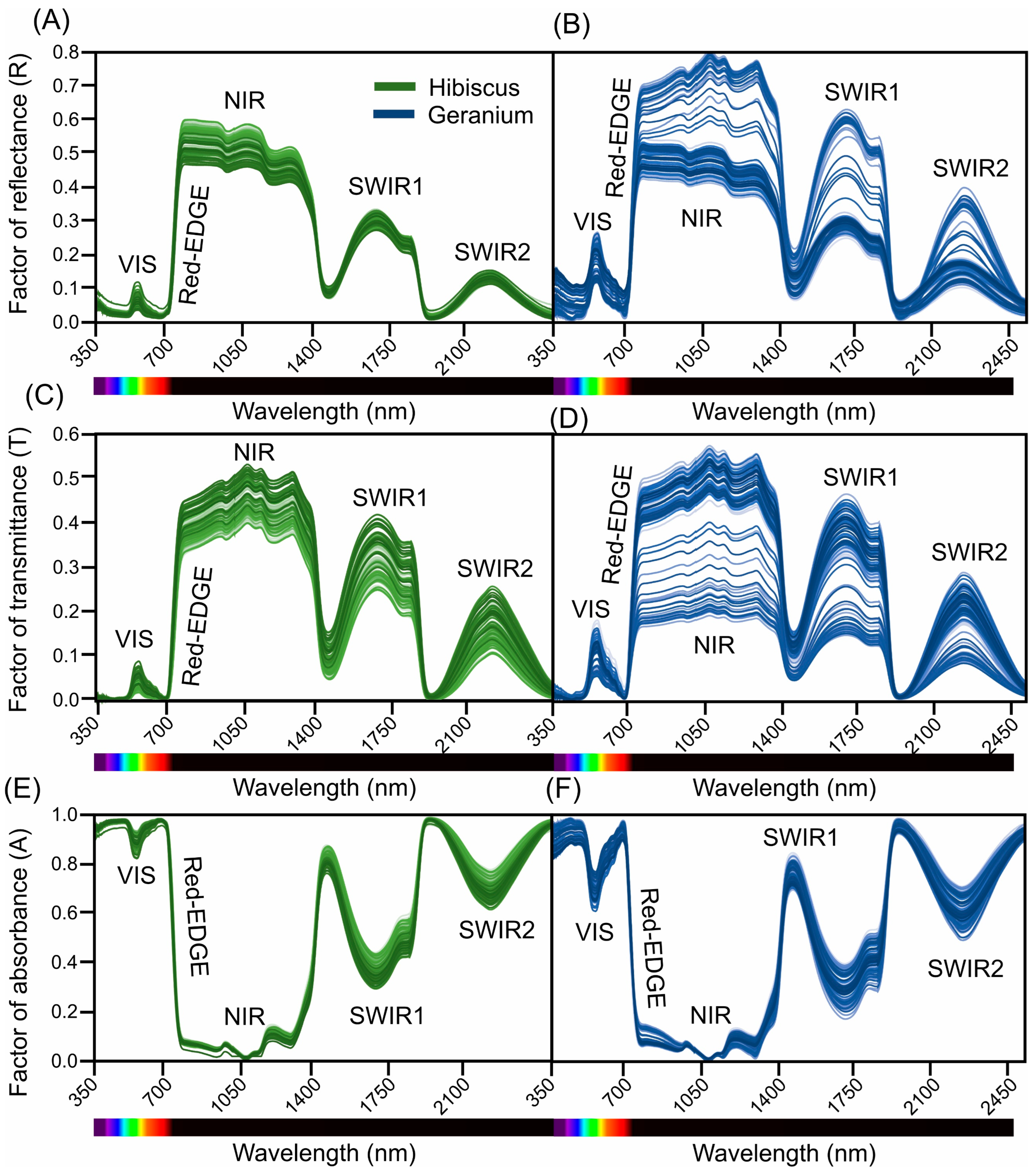
3.3. Hyperspectral Reflectance, Transmittance, and Absorbance Curves

Differences in reflectance values between Hibiscus and Geranium were observed at the responsive wavelengths across each spectral range (Figure 3A,B). In the VIS spectrum (400–700 nm), a notable disparity was evident at 544 nm. Within the NIR range (700–1300 nm), the most pronounced difference was observed at 700 nm. For the SWIR1 spectrum (1300–1800 nm), the peak difference was at 1441 nm, whereas in the SWIR2 range (1800–2500 nm), the largest variation was at 2488 nm. Given the consistently low p values (below 0.05) for these wavelengths, these differences are statistically significant, indicating that these specific wavelengths might be key in differentiating between Hibiscus and Geranium based on reflectance (Figure 3A,B).
Transmittance values also demonstrated significant variations between the two species at specific wavelengths in each spectral band (Figure 3C,D). In the VIS spectrum, the most marked difference was observed at 400 nm. In the NIR spectrum, the peak difference was at 1125 nm, in SWIR1, it was at 1607 nm, and in SWIR2, it peaked at 2175 nm. The notably low p values for these wavelengths affirm their statistical significance, suggesting that transmittance at these specific wavelengths can also differentiate between Hibiscus and Geranium plants (Figure 3C,D).
Absorbance analysis further revealed significant variations between Hibiscus and Geranium at distinct wavelengths across the spectral bands (Figure 3E,F). The most significant differences were observed at 495 nm in VIS_Blue, 498 nm in VIS_Green, 733 nm in VIS_Red, 800 nm in VIS_Far-red, 1117 nm in NIR, 1575 nm in SWIR1, and 2175 nm in SWIR2. The extremely low p values associated with these wavelengths confirm their statistical significance, indicating that absorbance at these wavelengths can be instrumental in distinguishing Hibiscus from Geranium plants (Figure 3E,F).

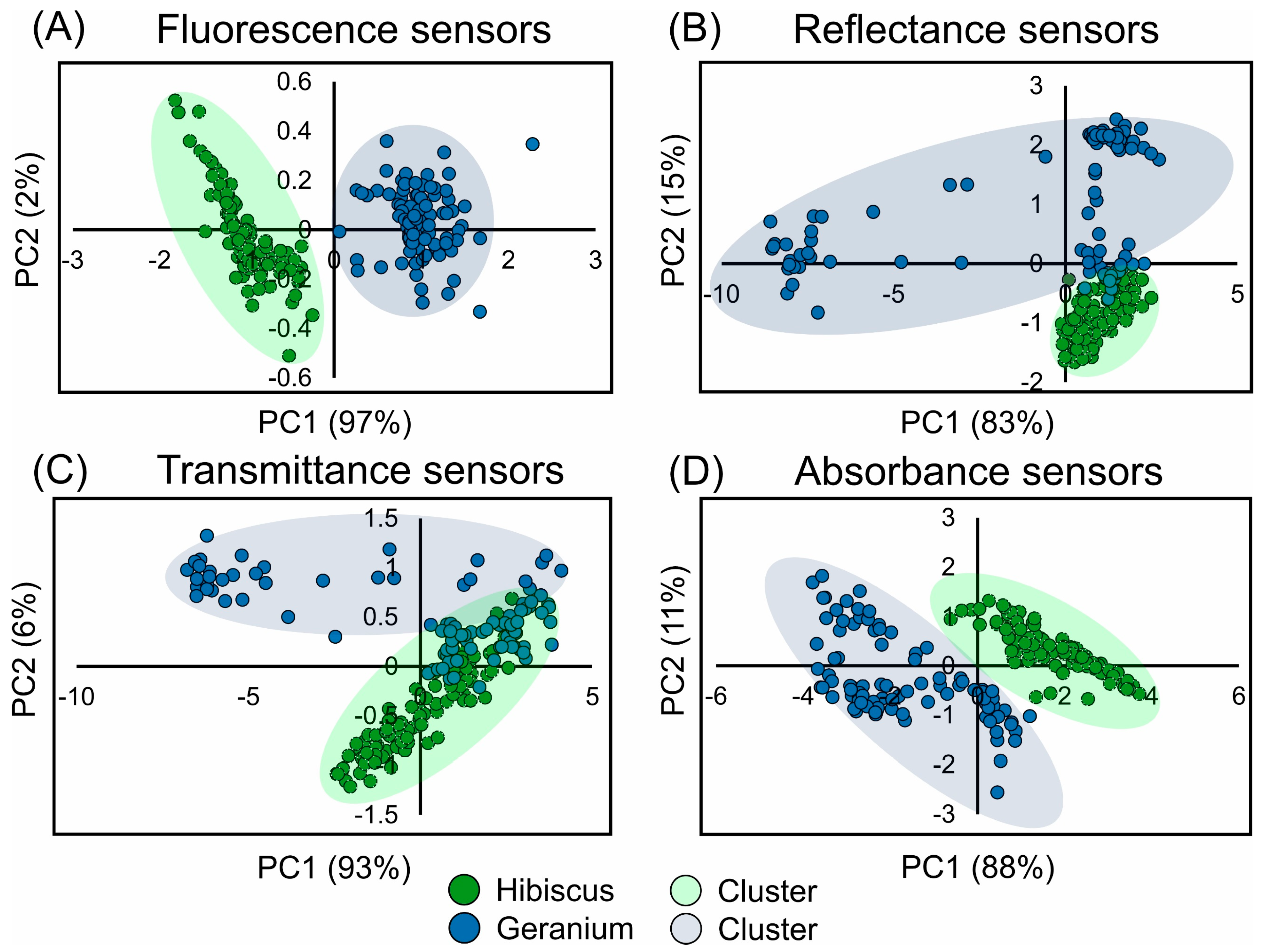
3.4. Principal Component Analysis for Fluorescence, Reflectance, Transmittance, and Absorbance Sensors

Utilizing the PERMANOVA, based on 999 permutations, a test statistic of 3.33 emerged for fluorescence curves, accompanied by a p value of 0.001. This underscores the distinctiveness between Hibiscus and Geranium fluorescence curves at a 95% confidence interval. The kappa coefficient (k) was 0.897, and the accuracy reached 0.948, suggesting 94.8% concordance when referencing the global average (Figure 4A).
For the reflectance curves, the PERMANOVA yielded a test statistic of 0.487. With a p value of 0.001, the discernible differences between both plants at a 95% confidence interval became evident. The kappa coefficient (k) was 0.852, indicating robust agreement. The accuracy metric, measured at 0.927, indicated that 92.7% of the wavelengths were harmoniously classified against the global mean (Figure 4B).
Addressing the transmittance curves, the PERMANOVA presented a test statistic of 0.246. This, coupled with a p value of 0.001, emphasizes the marked variations between the plants at the 95% confidence interval. A high kappa coefficient (k) of 0.978 was obtained. Furthermore, with an accuracy level of 0.987, a staggering 98.7% of wavelengths showed uniformity when juxtaposed with the global average (Figure 4C).
Regarding the absorbance curves, the analysis resulted in a test statistic of 1.215 and a p value of 0.001, indicating distinct differences at the 95% confidence level. A kappa coefficient (k) of 0.946 and an accuracy metric of 0.973 revealed that 97.3% of wavelengths were consistent when compared to the global mean (Figure 4D).
Within the reflectance data, the first principal component (PC-1) identified leading wavelengths at the blue bands at 450 nm, the green bands at 553 nm, the red bands at 572 nm, the NIR bands at 1276 nm, the SWIR1 bands at 1696 nm, and the SWIR2 bands at 2217 nm. Similar wavelengths were documented for PC-2 and PC-3 in the reflectance dataset (Figure 5).
In the transmittance spectrum for PC-1, relevant wavelengths were found in the blue bands at 452 nm, the green bands at 550 nm, the red bands at 670 nm, the NIR bands at 1060 nm, the SWIR1 bands at 1677 nm, and the SWIR2 bands at 2213 nm. Consequent PCs, PC-2 and PC-3 in the transmittance data, also pinpointed an array of pivotal wavelengths (Figure 5).
For the absorbance measurements, the foremost wavelengths for PC-1 included the blue range at 493 nm; the green range at 550 nm; the red range at 672 nm; the NIR range at 713 nm; the SWIR1 range at 1829 nm and 1835 nm; and the SWIR2 range at 2247 nm. The absorbance results for PC-2 and PC-3 also revealed key wavelengths (Figure 5).
These findings align with the regression coefficients and provide insights into the most influential wavelengths across the reflectance, transmittance, and absorbance spectra.

3.5. Selection of Variables by PLS Algorithms for Hyperspectral Vegetation Index

The reflectance dataset reveals distinct regions with high correlation (Figure 6), marked by red indicators, especially within specific wavelength bands. This pronounced correlation is evident at the outset of the spectrum, primarily within the visible (VIS) range. Additionally, such correlation patterns are identifiable in selected areas of both the near-infrared (NIR) and shortwave infrared (SWIR) spectra. In contrast, the spectrum showcases sporadic sections, delineated in blue, where correlation is either minimal or absent. These low-correlation zones predominantly appear around the midpoint of the spectrum and within certain segments of the SWIR (Figure 6) or Ψ(RO), ϕ(RO), and Kn (Figure 6B,E,I) with low values (p > 0.05).
In the transmittance dataset (Figure 7), it is discernible that areas of high correlation predominantly cluster at the spectrum’s onset, specifically in the visible domain, and are also present within defined bands of the NIR. Scattered peaks within the SWIR further substantiate this observation. However, as one navigates through the remainder of the spectrum, especially within the SWIR realm, the trend veers towards a low to nonexistent correlation (Figure 7) or Ψ(RO), ϕ(RO), and Kn (Figure 7B,E,I) with low values (p > 0.05).
In the context of the absorbance dataset (Figure 8), the data suggest substantial correlations pervading numerous sections of the spectrum, particularly in the VIS and NIR regions. The consistency in the distribution of these high-correlation regions, accentuated in red, stands in stark contrast with the other datasets. However, it is essential to acknowledge the less pervasive yet discernible regions of diminished correlation, primarily situated within certain SWIR stretches or Ψ(RO), ϕ(RO), and Kn (Figure 8B,E,I) with low values (p > 0.05).
Based on these observations, the visual data shows that wavelengths within the VIS and NIR, as well as VIS and SWIR2, exhibit a robust correlation with hyperspectral vegetation indices (HVIs) across the three examined datasets, which include hyperspectral sensors measuring reflectance, transmittance, and absorbance. The SWIR spectrum provides some relevance in characterizing ChlF parameters, unveiling a dichotomy of high and low correlations, contingent on the dataset and the specific SWIR segment. Notably, of all the datasets, the absorbance one elucidates the most balanced distribution of prominent correlations throughout the spectrum, with its counterparts, reflectance and transmittance, presenting a more varied distribution (Figure 6, Figure 7 and Figure 8).

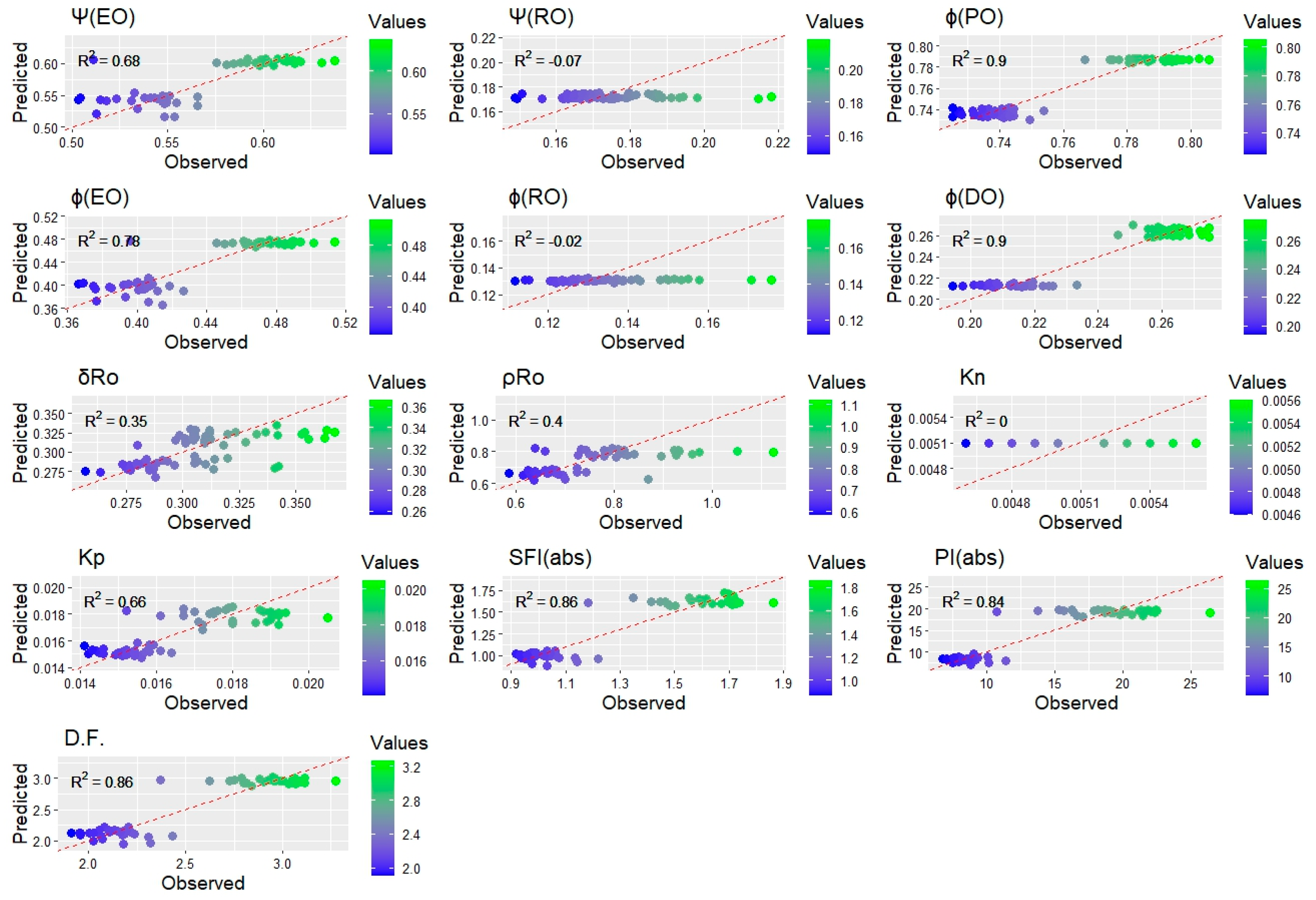
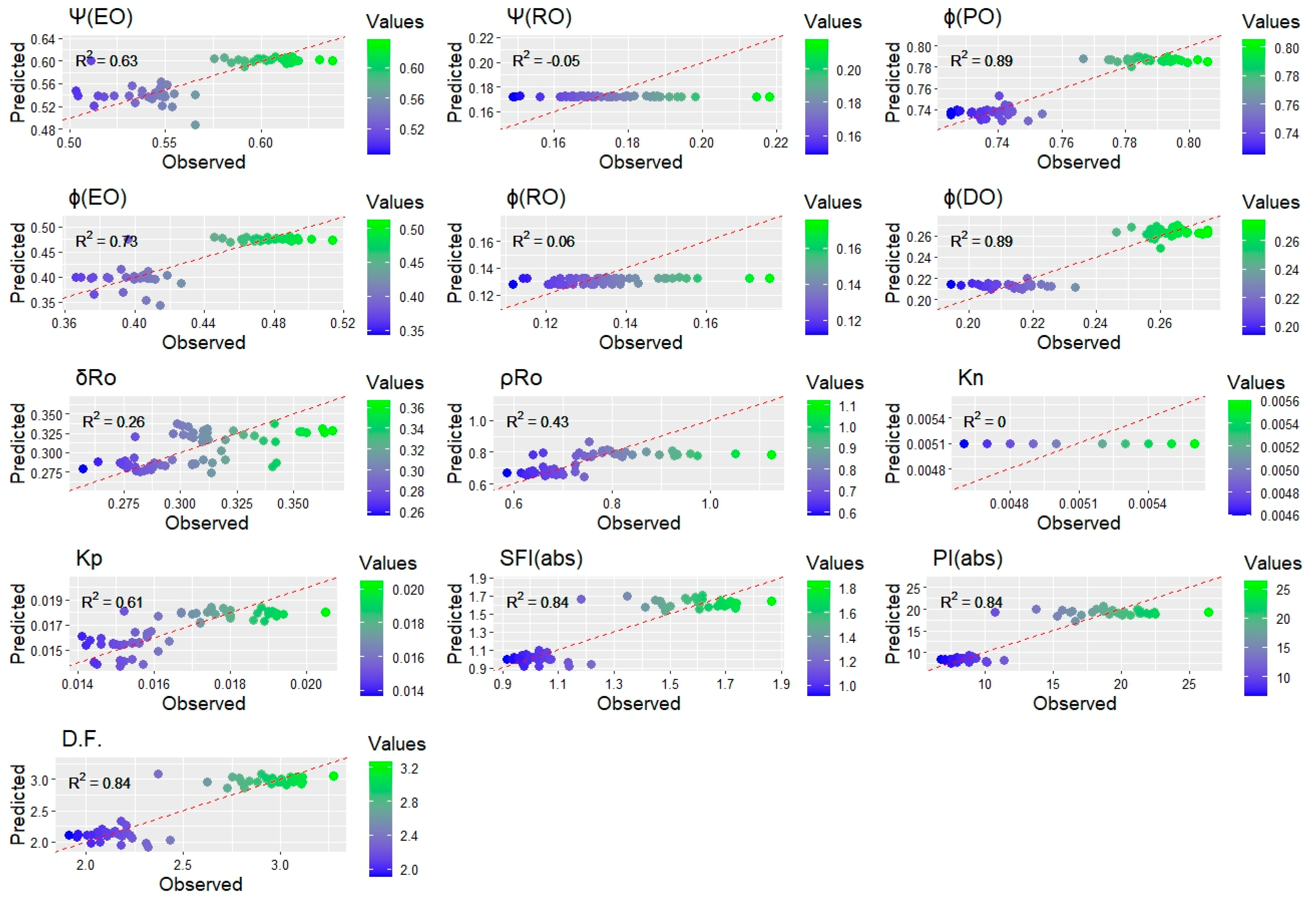
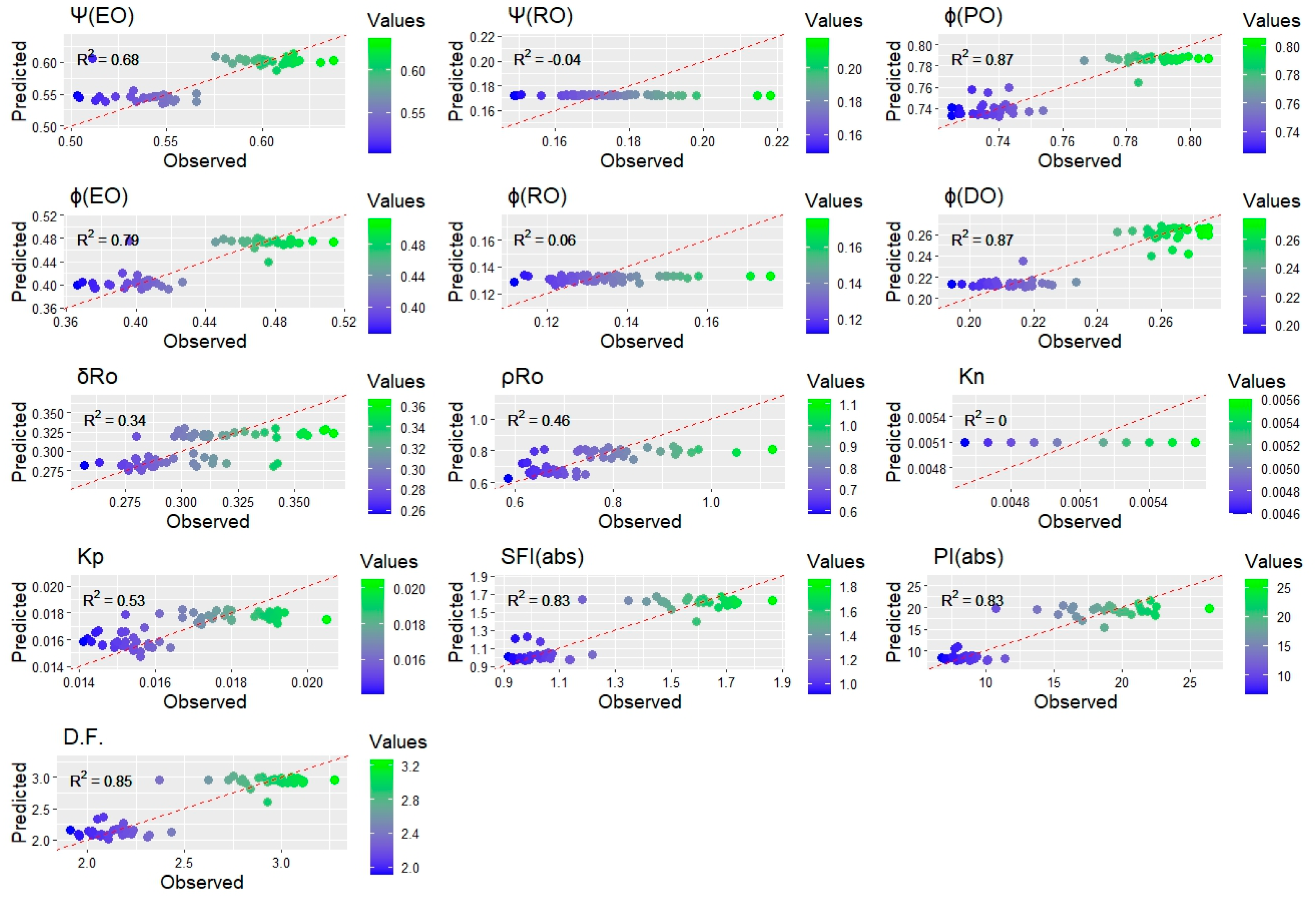
3.6. Chlorophyll a Fluorescence Predicted Parameters

3.6.1. Calibration and Validation Models

Our research delved deeply into a comprehensive evaluation of three spectrometric modalities: reflectance, transmittance, and absorbance (Table 2). Reflectance, which focuses on the fraction of light or radiation reflected by a material while excluding the absorbed portions, revealed several distinct outcomes. Higher performers in this category include ϕ(PO) due to its R2 values of 0.86 in calibration and 0.83 in cross-validation. This, combined with a consistently minimized RMSE, suggests an effective model adept at capturing intrinsic variance. The ratio of performance to deviation (RPD) further underscores these parameters (Table 2).
The most notable performers in the reflectance modality were Ψ(EO) and ϕ(EO). Both displayed R2 values, with Ψ(EO) at 0.77 for calibration and 0.75 for cross-validation and ϕ(EO) at 0.81 and 0.77, respectively. Their associated RMSE values support their model’s precision. Another parameter, ϕ(DO), with an R2 of 0.85 for calibration and 0.82 for cross-validation, confirms its significant contribution to reflectance assessments. Meanwhile, parameters such as δRo, ρRo, Kn, Kp, SFI(abs), and PI(abs) exhibited moderate R2 values. Here, δRo and ρRo indicate potential areas for optimization. Interestingly, despite high R2 values, parameters such as Kn were highlighted because of their minor inconsistencies in cross-validation metrics. On the other end of the spectrum, parameters Ψ(RO) and ϕ(RO) had the lowest accuracy (p > 0.05). Showing considerably low R2 values and Ψ(RO) notably missing cross-validation results while ϕ(RO) show 0.12 in calibration, there are significant concerns regarding their efficacy in reflectance assessments.
It is evident that the transmittance sensor, which quantifies the fraction of light passing through a medium, is a critical facet of spectrometry. Leading the pack here are ϕ(PO) and ϕ(DO). They had R2 values of ≈0.89 and 0.86 for calibration and cross-validation, respectively, which show higher predictive capabilities. Ψ(EO), ϕ(EO), Kn, SFI(abs), and PI(abs) also emerge as trustworthy assets in transmittance evaluations, with their R2 values oscillating between 0.70 and 0.89 during calibration. However, δRo, ρRo, and Kp, despite their promise, disclosed disparities between calibration and cross-validation, hinting at enhancement opportunities. Conversely, the recurring underperformance of Ψ(RO) and ϕ(RO) is the lowest, especially given the low R2 value of 0.01 for Ψ(RO), which questions its aptness in transmittance evaluations (Table 2).
Last, in the context of absorbance, where the central task is gauging the amount of light absorbed by leaves, ϕ(PO) and ϕ(DO) continue their consistent streak. Both R2 values approach or exceed 0.82, accentuating their dominant role in absorbance evaluations. Similarly, parameters such as Ψ(EO), ϕ(EO), Kn, SFI(abs), and D.F., with R2 values in the vicinity of mid−0.7 s to mid−0.8 s, confirm their steadfastness in absorbance evaluations. ρRo, Kp, and PI(abs) provided acceptable calibration results, but their minor deviations in the cross-validation data suggest room for improvement. Once again, the performance of Ψ(RO) and ϕ(RO) is low for this modality, with their significantly lower R2 values (Table 2).

3.6.2. Predicted

Reflectance quantifies the light or radiation that bounces off a material (Table 3). Certain high-precision predictors have emerged prominently in assessing the predictive performance of various parameters. For instance, Ψ(EO) exhibited a correlation coefficient (R2) of 0.84, augmented with an SEP of 0.01 and an RPD of 1.84, highlighting its remarkable prediction accuracy. ϕ(EO) and ϕ(DO), with r values of 0.86 and 0.85, respectively, and RPDs of 1.96 and 1.91, further underscored superior predictive abilities. Additionally, SFI(abs) made a notable mark with an R2 value of 0.90 and an RPD of 2.32 (Table 3; reflectance data).
Stable performers, such as ϕ(PO), δRo, ρRo, Kn, Kp, and D.F., registered R2 values between 0.50 and 0.88, indicating their reliable predictive behavior. Conversely, parameters such as Ψ(RO) and ϕ(RO), with r values of −0.02 and 0.22 and RPDs of 1.00 and 1.02, respectively, pinpoint areas needing refinement or select few bands to enhance correlations and R2 and RPD metrics (Table 3; reflectance).
Transmittance denotes the fraction of light traversing a medium. High-precision predictors in this category included Ψ(EO), ϕ(PO), ϕ(EO), and ϕ(DO), all presenting R2 values above 0.90 and RPDs between 2.27 and 2.68. SFI(abs) distinguished itself with an exceptional R2 value of 0.95 and an RPD of 3.32 (Table 3; transmittance).
Other consistently performing predictors, namely, δRo, ρRo, Kn, Kp, and D.F., showed R2 values from 0.49 to 0.95. However, the effectiveness of Ψ(RO) in transmittance prediction warrants scrutiny given its R2 value of 0.03 and an RPD of approximately 1.00 (Table 3; transmittance data).
For absorbance, which measures the amount of light absorbed, many high-precision predictors were evident (Table 3; absorbance data). Ψ(EO), ϕ(EO), and ϕ(DO) all had R2 values ranging from 0.86 to 0.88 and RPDs surpassing 1.95, affirming their higher prediction capabilities for absorbance. SFI(abs) further stood out with an R2 value of 0.91 and an RPD of 2.45. While ϕ(PO), δRo, ρRo, Kn, Kp, and D.F. showcased R2 values between 0.48 and 0.90, highlighting predictive abilities, Ψ(RO) left room for enhancement, registering an R2 value of 0.03 and an RPD marginally over one, signaling potential prediction challenges (Table 3; absorbance data).
Scatter plot data between predicted and observed values revealed that the data obtained by absorbance were more consistent and larger in comparison to reflectance and transmittance data (p < 0.01) (Figure 9, Figure 10 and Figure 11).
The scatter plots for reflectance display a wide dispersion of points, suggesting a lower consistency between observed and predicted values for various variables (Figure 9). Variables such as Ψ(EO) and ϕ(PO) show moderate correlations, whereas δRo and SFI(abs) have weaker correlations. The color gradient, transitioning from blue to green, signifies correlation strength, with blue being associated with low values and green with high values.
Transmittance scatter plots also show a broad dispersion of points, with some variables, such as ϕ(RO) and PI(abs), displaying moderate correlations, whereas others, such as Ψ(RO) and Kn, present weaker correlations (Figure 10).
In contrast, the absorbance scatter plots revealed a tighter clustering of points around a 1:1 line, indicating a robust and consistent correlation between the observed and predicted values (Figure 11). The intensity of the colors leans more towards green, suggesting stronger correlations compared to reflectance and transmittance sensors.
In summary, absorbance is the most reliable method for predicting plant characteristics among the three, with reflectance and transmittance showing the greatest variability in their predictions.

4. Discussion

The application of hyperspectral sensors in predicting chlorophyll a fluorescence parameters has gained considerable attention in recent plant physiological research (Figure 1, Figure 2, Figure 3, Figure 4, Figure 5, Figure 6, Figure 7, Figure 8, Figure 9, Figure 10 and Figure 11) [4,6,13]. The interactions between light and plant tissues, including absorption, reflection, and transmission, provide valuable insights beyond the superficial health of plants. They reveal crucial physiological processes and adaptive mechanisms. This section critically evaluates the present research findings in the context of established scientific knowledge.

4.1. Insights into Chlorophyll a Fluorescence Parameters

Chlorophyll a fluorescence is a noninvasive technique that is widely accepted for evaluating photosystem II (PSII) functionality and the overall physiological status of a plant [32,33]. The variations observed between Hibiscus and Geranium in their OJIP test parameters underscore the inherent species-specific characteristics of photochemical processes.
In this context, prediction data with high coefficients of variation (CV %) and maximum and minimum values should be evaluated to understand whether hyperspectral curves are capable of capturing this information using most of the electromagnetic spectrum [34,35]. This approach aligns with the growing interest in hyperspectral imaging for plant phenotyping, which provides detailed information on plant health and photosynthetic performance [3,36]. However, it is important to note that while hyperspectral data can provide valuable insights into plant health and physiology, the interpretation of these data requires a thorough understanding of both the underlying biological processes and the technical aspects of hyperspectral imaging and nonimaging [37]. Therefore, careful analysis and interpretation of hyperspectral data are key to the accurate prediction of plant traits and the assessment of plant health [26,38,39,40,41]. For example, understanding the species-specific characteristics of photochemical processes using techniques such as chlorophyll a fluorescence can provide valuable insights into plant physiology [6,29]. When combined with advanced imaging techniques such as hyperspectral imaging, it can potentially enhance our ability to monitor plant health and predict plant traits. However, further research is required to improve the accuracy and reliability of these methods.
In this sense, the elevated fluorescence intensities at the L, K, J, and I points in Geranium might be attributed to the early phases of electron transfer. These variations could potentially be linked to mechanisms such as nonphotochemical quenching or changes in electron transport rates (Figure 2; Table 2 and Table 3).

4.2. Hyperspectral and Principal Component Analysis by Reflectance, Transmittance, and Absorbance

Hyperspectral sensors offer in-depth spectral data, enabling a thorough analysis of plant biochemical and biophysical characteristics [7]. Reflectance provides information about the surface and internal structure of leaves [42]. Changes in reflectance patterns can indicate variations in chlorophyll concentration or cellular modifications, as supported by previous studies [43,44]. Transmittance patterns are valuable for understanding light diffusion within the leaf, reinforcing the findings of [45,46]. The large datasets derived from hyperspectral sensors necessitate the use of dimensionality reduction techniques such as principal component analysis (PCA). This research successfully employed PCA to identify vital spectral regions associated with variations in chlorophyll a fluorescence parameters. Identifying these regions is crucial for the development of effective remote sensing tools, a concept also emphasized by [28,47].
In this context, prediction data with high coefficients of variation (CV %) and maximum and minimum values should be evaluated to understand whether hyperspectral curves are indeed capable of capturing this information, using most of the electromagnetic spectrum (Figure 3 and Figure 4). This approach aligns with the growing interest in using hyperspectral imaging for plant phenotyping, which provides detailed information about plant health and photosynthetic performance (Figure 2, Figure 5, Figure 6, Figure 7, Figure 8 and Figure 9 and Table 2 and Table 3). However, it is important to note that while hyperspectral data can provide valuable insights into plant health and physiology, the interpretation of these data requires a thorough understanding of both the underlying biological processes and the technical aspects of hyperspectral imaging. Therefore, careful analysis and interpretation of hyperspectral data are crucial for accurate prediction of plant monitoring [5,16,28,48].
The parameters Ψ(EO), Ψ(RO), ϕ(PO), ϕ(EO), ϕ(RO), ϕ(DO), δRo, ρRo, Kn, Kp, SFI(abs), PI(abs), and D.F. (JIP-test) are all parameters that can be derived from the JIP-test, which quantifies PSII performance [21,49]. These parameters can provide valuable insights into various aspects of photosynthetic performance and plant health. For example, Ψ(EO) and ϕ(PO) have been shown to be sensitive indicators of changes in photosynthetic efficiency, whereas δRo and SFI(abs) can provide information regarding energy dissipation mechanisms within the photosystem [50,51].
By correlating these parameters with hyperspectral data, it may be possible to develop predictive models that can estimate them based on hyperspectral measurements (Figure 1, Figure 2, Figure 3, Figure 4, Figure 5, Figure 6, Figure 7, Figure 8, Figure 9, Figure 10 and Figure 11). For example, despite the use of hyperspectral imaging sensors, advancements in this quantification could be explored using hyperspectral cameras or perhaps with the use of multispectral sensors.

4.3. Predictive Modeling-Based Reflectance, Transmittance, and Absorbance

By integrating hyperspectral sensors with partial least squares (PLS) algorithms, we can effectively predict parameters such as chlorophyll a fluorescence. This parameter is a vital indicator of photosynthetic performance and the electron transport chain [13].
Both variable importance in projection (VIP) and hyperspectral vegetation indices (HVIs) are pivotal tools in hyperspectral data analysis. They serve as dependable selectors of the wavelength, significantly enhancing the predictive accuracy of the models. These methodologies adeptly pinpoint the key spectral regions rich in significant information, thereby aiding in the understanding of various plant characteristics. Consequently, their combined use paves the way for more accurate and holistic assessments (Figure 3 and Figure 5).
Given the vast amount of data generated by hyperspectral sensors, it is imperative to employ dimensionality reduction techniques, such as principal component analysis (PCA). PCA, in particular, excels at identifying the essential spectral regions associated with variations in chlorophyll a fluorescence parameters. Recognizing these regions is crucial for crafting proficient remote sensing tools specifically designed to estimate plant properties such as chlorophyll, nitrogen content, and JIP-test parameters, which include thermal dissipation and electron flow in the electron transport chain.
Calibration and validation models stemming from this synergistic approach not only facilitate real-time analysis but also highlight the potential of remote sensing in large-scale monitoring. This is in line with current viewpoints that emphasize the revolutionary potential of remote sensing technologies for globally monitoring and managing plant health and productivity [47,52]. By delivering timely and accurate data on plant health, these technologies have the potential to influence decision-making in areas such as agriculture, forestry, and other sectors related to remote sensing, guiding them toward enhanced productivity and sustainability.
Therefore, although predictive modeling utilizing hyperspectral data holds immense potential to enhance our understanding of plant health and physiology, ongoing research is essential. Deepening our insights will not only refine these methods but also extend their use across a range of plant species and environmental settings. With the ongoing progress in the field, noninvasive plant health assessments are poised to become indispensable in sustainable practices, especially when analyzing reflectance, transmittance, and absorbance sensors simultaneously [13].
Whole-spectrum-based models such as PLSR, LDA, and SVR excel at classifying and predicting leaf properties, offering invaluable insights for interpreting chlorophyll a fluorescence data, which are crucial for JIP-test evaluations [5,16,28,48]. These models capitalize on the full spectrum of available data, ensuring a nuanced understanding of intricate leaf attributes, including interactions in leaf optical properties and the complex chemistry involving various molecules associated with photosystems and the electron transport chain. The detailed spectral analysis is integral to a comprehensive understanding of the complex interplay between leaf biochemical compositions, including proteins and other molecules to photosystems. In the realm of chlorophyll a fluorescence data, the depth and breadth of insights offered by whole-spectrum approaches are pivotal [21,49]. While VIS and VIs simplify computational demands, they compromise on the richness of data, potentially overlooking critical insights. Whole-spectrum models counter this limitation, offering enhanced accuracy and reliability in assessing chlorophyll a fluorescence, thus amplifying the depth of insights gleaned from JIP-test data evaluations.

5. Conclusions

This study examined the use of hyperspectral sensors to predict chlorophyll a fluorescence parameters, emphasizing their role in gauging photosynthetic efficiency in Hibiscus and Geranium. The data revealed a clear correlation between hyperspectral readings and ChlF parameters. The developed models were highly precise, highlighting the effectiveness of the employed multivariate statistical methods. The spectral regions linked to these parameters, ranging from blue to shortwave infrared, are vital for noninvasive assessments of plant physiology.
The use of the hyperspectral vegetation indices (HVIs) tool was essential in selecting wavelengths, which led to improved outcomes in the partial least squares (PLS) models. The accuracy achieved by these models indicates the promising role of hyperspectral sensors in understanding plant photosynthesis.
For subsequent studies, it would be beneficial to study a wider variety of plant species and to incorporate additional methods. This enhances the accuracy and relevance of the hyperspectral sensors in plant biology. Furthermore, testing this approach in diverse field settings may provide more clarity on its consistency and versatility.

Author Contributions

Conceptualization, R.F. and M.R.N.; Data curation, R.F. and M.R.N.; Formal analysis, R.F., R.B.d.O., M.L.C., J.A.M.D. and M.R.N.; Funding acquisition, R.F., R.B.d.O., J.A.M.D. and M.R.N.; Investigation, R.F., W.C.A., R.B.d.O., M.L.C., J.A.M.D. and M.R.N.; Methodology, R.F., W.C.A., R.B.d.O., M.L.C. and M.R.N.; Project administration, R.F. and M.R.N.; Resources, R.F. and M.R.N.; Software, R.F., W.C.A., R.B.d.O., M.L.C., J.A.M.D. and M.R.N.; Supervision, R.F. and M.R.N.; Validation, R.F., R.B.d.O., M.L.C., J.A.M.D. and M.R.N.; Visualization, R.F. and M.R.N.; Writing—original draft, R.F., W.C.A., R.B.d.O., M.L.C., J.A.M.D. and M.R.N.; Writing—review and editing, R.F. and M.R.N. All authors have read and agreed to the published version of the manuscript.

Funding

National Council for Scientific and Technological Development: Programa de Apoio à Fixação de Jovens Doutores no Brasil 168180/2022−7; Fundação Araucária: CP 19/2022—Jovens Doutores; Coordenação de Aperfeiçoamento de Pessoal de Nível Superior: 001; Fundação de Amparo à Pesquisa do Estado de São Paulo, FAPESP pn 2021/05129−8 for sensor financial support. CEAGRE—Centro de Excelência em Agricultura Exponencial for financial support.

Institutional Review Board Statement

Not applicable.

Informed Consent Statement

Not applicable.

Data Availability Statement

Not applicable.

Acknowledgments

We also thank Programa de Pós-Graduação em Agronomia (PGA-UEM) at the State University of Maringá and FAPESP for their support.

Conflicts of Interest

The authors declare no conflict of interest. The funders had no role in the design of the study; in the collection, analyses, or interpretation of data; in the writing of the manuscript; or in the decision to publish the results.

References

  1. Falcioni, R.; Moriwaki, T.; Bonato, C.M.; de Souza, L.A.; Nanni, M.R.; Antunes, W.C. Distinct Growth Light and Gibberellin Regimes Alter Leaf Anatomy and Reveal Their Influence on Leaf Optical Properties. Environ. Exp. Bot. 2017, 140, 86–95. [Google Scholar] [CrossRef]
  2. Fankhauser, C.; Chory, J. Light Control of Plant Development. Annu. Rev. Cell Dev. Biol. 1997, 13, 203–229. [Google Scholar] [CrossRef] [PubMed]
  3. Kováč, D.; Veselovská, P.; Klem, K.; Večeřová, K.; Ač, A.; Peñuelas, J.; Urban, O. Potential of Photochemical Reflectance Index for Indicating Photochemistry and Light Use Efficiency in Leaves of European Beech and Norway Spruce Trees. Remote Sens. 2018, 10, 1202. [Google Scholar] [CrossRef]
  4. Cotrozzi, L.; Lorenzini, G.; Nali, C.; Pellegrini, E.; Saponaro, V.; Hoshika, Y.; Arab, L.; Rennenberg, H.; Paoletti, E. Hyperspectral Reflectance of Light-Adapted Leaves Can Predict Both Dark- and Light-Adapted Chl Fluorescence Parameters, and the Effects of Chronic Ozone Exposure on Date Palm (Phoenix dactylifera). Int. J. Mol. Sci. 2020, 21, 6441. [Google Scholar] [CrossRef] [PubMed]
  5. Murchie, E.H.; Lawson, T. Chlorophyll Fluorescence Analysis: A Guide to Good Practice and Understanding Some New Applications. J. Exp. Bot. 2013, 64, 3983–3998. [Google Scholar] [CrossRef] [PubMed]
  6. Falcioni, R.; Moriwaki, T.; Antunes, W.C.; Nanni, M.R. Rapid Quantification Method for Yield, Calorimetric Energy and Chlorophyll a Fluorescence Parameters in Nicotiana tabacum L. Using Vis-NIR-SWIR Hyperspectroscopy. Plants 2022, 11, 2406. [Google Scholar] [CrossRef] [PubMed]
  7. Vilfan, N.; van der Tol, C.; Muller, O.; Rascher, U.; Verhoef, W. Fluspect-B: A Model for Leaf Fluorescence, Reflectance and Transmittance Spectra. Remote Sens. Environ. 2016, 186, 596–615. [Google Scholar] [CrossRef]
  8. Falcioni, R.; dos Santos, G.L.A.A.; Crusiol, L.G.T.; Antunes, W.C.; Chicati, M.L.; de Oliveira, R.B.; Demattê, J.A.M.; Nanni, M.R. Non-Invasive Assessment, Classification, and Prediction of Biophysical Parameters Using Reflectance Hyperspectroscopy. Plants 2023, 12, 2526. [Google Scholar] [CrossRef]
  9. Asner, G.P.; Jones, M.O.; Martin, R.E.; Knapp, D.E.; Hughes, R.F. Remote Sensing of Native and Invasive Species in Hawaiian Forests. Remote Sens. Environ. 2008, 112, 1912–1926. [Google Scholar] [CrossRef]
  10. Sobejano-Paz, V.; Mikkelsen, T.N.; Baum, A.; Mo, X.; Liu, S.; Köppl, C.J.; Johnson, M.S.; Gulyas, L.; García, M. Hyperspectral and Thermal Sensing of Stomatal Conductance, Transpiration, and Photosynthesis for Soybean and Maize under Drought. Remote Sens. 2020, 12, 3182. [Google Scholar] [CrossRef]
  11. Nalepa, J. Recent Advances in Multi and Hyperspectral Image Analysis. Sensors 2021, 21, 6002. [Google Scholar] [CrossRef] [PubMed]
  12. Kior, A.; Sukhov, V.; Sukhova, E. Application of Reflectance Indices for Remote Sensing of Plants and Revealing Actions of Stressors. Photonics 2021, 8, 582. [Google Scholar] [CrossRef]
  13. Falcioni, R.; Antunes, W.C.; Demattê, J.A.M.; Nanni, M.R. Biophysical, Biochemical, and Photochemical Analyses Using Reflectance Hyperspectroscopy and Chlorophyll a Fluorescence Kinetics in Variegated Leaves. Biology 2023, 12, 704. [Google Scholar] [CrossRef] [PubMed]
  14. Fan, K.; Li, F.; Chen, X.; Li, Z.; Mulla, D.J. Nitrogen Balance Index Prediction of Winter Wheat by Canopy Hyperspectral Transformation and Machine Learning. Remote Sens. 2022, 14, 3504. [Google Scholar] [CrossRef]
  15. Crusiol, L.G.T.; Sun, L.; Sun, Z.; Chen, R.; Wu, Y.; Ma, J.; Song, C. In-Season Monitoring of Maize Leaf Water Content Using Ground-Based and UAV-Based Hyperspectral Data. Sustainability 2022, 14, 9039. [Google Scholar] [CrossRef]
  16. Martinez-Nolasco, C.; Padilla-Medina, J.A.; Nolasco, J.J.M.; Guevara-Gonzalez, R.G.; Barranco-Gutiérrez, A.I.; Diaz-Carmona, J.J. Non-Invasive Monitoring of the Thermal and Morphometric Characteristics of Lettuce Grown in an Aeroponic System through Multispectral Image System. Appl. Sci. 2022, 12, 6540. [Google Scholar] [CrossRef]
  17. Kusaka, M.; Kalaji, H.M.; Mastalerczuk, G.; Dabrowski, P.; Kowalczyk, K. Potassium Deficiency Impact on the Photosynthetic Apparatus Efficiency of Radish. Photosynthetica 2021, 59, 127–136. [Google Scholar] [CrossRef]
  18. Mendes Bezerra, A.C.; da Cunha Valença, D.; da Gama Junqueira, N.E.; Moll Hüther, C.; Borella, J.; Ferreira de Pinho, C.; Alves Ferreira, M.; Oliveira Medici, L.; Ortiz-Silva, B.; Reinert, F. Potassium Supply Promotes the Mitigation of NaCl-Induced Effects on Leaf Photochemistry, Metabolism and Morphology of Setaria Viridis. Plant Physiol. Biochem. 2021, 160, 193–210. [Google Scholar] [CrossRef]
  19. Bauriegel, E.; Giebel, A.; Herppich, W.B. Hyperspectral and Chlorophyll Fluorescence Imaging to Analyse the Impact of Fusarium Culmorum on the Photosynthetic Integrity of Infected Wheat Ears. Sensors 2011, 11, 3765–3779. [Google Scholar] [CrossRef]
  20. Jia, M.; Li, D.; Colombo, R.; Wang, Y.; Wang, X.; Cheng, T.; Zhu, Y.; Yao, X.; Xu, C.; Ouer, G.; et al. Quantifying Chlorophyll Fluorescence Parameters from Hyperspectral Reflectance at the Leaf Scale under Various Nitrogen Treatment Regimes in Winter Wheat. Remote Sens. 2019, 11, 2838. [Google Scholar] [CrossRef]
  21. Schansker, G.; Tóth, S.Z.; Strasser, R.J. Dark Recovery of the Chl a Fluorescence Transient (OJIP) after Light Adaptation: The QT-Component of Non-Photochemical Quenching Is Related to an Activated Photosystem I Acceptor Side. Biochim. Biophys. Acta-Bioenerg. 2006, 1757, 787–797. [Google Scholar] [CrossRef] [PubMed]
  22. Gao, Y.; Liu, W.; Wang, X.; Yang, L.; Han, S.; Chen, S.; Strasser, R.J.; Valverde, B.E.; Qiang, S. Comparative Phytotoxicity of Usnic Acid, Salicylic Acid, Cinnamic Acid and Benzoic Acid on Photosynthetic Apparatus of Chlamydomonas Reinhardtii. Plant Physiol. Biochem. 2018, 128, 1–12. [Google Scholar] [CrossRef]
  23. Strasser, R.J.; Michael, M.T. Analysis of the Fluorescence Transient Alaka Srivastava Summary II. The Theoretical Background. In Chlorophyll a Fluorescence 23; 2005. [Google Scholar]
  24. Strasser, R.J.; Srivastava, A.; Tsimilli-Michael, M. The Fluorescence Transient as a Tool to Characterize and Screen Photosynthetic Samples. Probing Photosynth. Mech. Regul. Adapt. 2000, 25, 443–480. [Google Scholar]
  25. Minasny, B.; McBratney, A.B.; Malone, B.P.; Wheeler, I. Digital Mapping of Soil Carbon. In Advances in Agronomy; Academic Press: Cambridge, MA, USA, 2013; Volume 3, pp. 1–47. [Google Scholar]
  26. Fernandes, A.M.; Fortini, E.A.; Müller, L.A.d.C.; Batista, D.S.; Vieira, L.M.; Silva, P.O.; do Amaral, C.H.; Poethig, R.S.; Otoni, W.C. Leaf Development Stages and Ontogenetic Changes in Passionfruit (Passiflora Edulis Sims.) Are Detected by Narrowband Spectral Signal. J. Photochem. Photobiol. B Biol. 2020, 209, 111931. [Google Scholar] [CrossRef] [PubMed]
  27. Yoosefzadeh-Najafabadi, M.; Tulpan, D.; Eskandari, M. Using Hybrid Artificial Intelligence and Evolutionary Optimization Algorithms for Estimating Soybean Yield and Fresh Biomass Using Hyperspectral Vegetation Indices. Remote Sens. 2021, 13, 2555. [Google Scholar] [CrossRef]
  28. Crusiol, L.G.T.; Nanni, M.R.; Furlanetto, R.H.; Sibaldelli, R.N.R.; Sun, L.; Gonçalves, S.L.; Foloni, J.S.S.; Mertz-Henning, L.M.; Nepomuceno, A.L.; Neumaier, N.; et al. Assessing the Sensitive Spectral Bands for Soybean Water Status Monitoring and Soil Moisture Prediction Using Leaf-Based Hyperspectral Reflectance. Agric. Water Manag. 2023, 277, 108089. [Google Scholar] [CrossRef]
  29. Falcioni, R.; Moriwaki, T.; Gibin, M.S.; Vollmann, A.; Pattaro, M.C.; Giacomelli, M.E.; Sato, F.; Nanni, M.R.; Antunes, W.C. Classification and Prediction by Pigment Content in Lettuce (Lactuca sativa L.) Varieties Using Machine Learning and ATR-FTIR Spectroscopy. Plants 2022, 11, 3413. [Google Scholar] [CrossRef]
  30. Zar, J.H. Biostatistical Analysis, 5th ed.; Pearson Education: Upper Saddle River, NJ, USA, 2010; ISBN 0-13-100846-3. [Google Scholar]
  31. Falcioni, R.; Antunes, W.C.; Demattê, J.A.M.; Nanni, M.R. Reflectance Spectroscopy for the Classification and Prediction of Pigments in Agronomic Crops. Plants 2023, 12, 2347. [Google Scholar] [CrossRef]
  32. Cuchiara, C.C.; Silva, I.M.C.; Dalberto, D.S.; Bacarin, M.A.; Peters, J.A. Chlorophyll a Fluorescence in Sweet Potatoes under Different Copper Concentrations. J. Soil Sci. Plant Nutr. 2015, 15, 179–189. [Google Scholar] [CrossRef]
  33. Kalt, W.; Cassidy, A.; Howard, L.R.; Krikorian, R.; Stull, A.J.; Tremblay, F.; Zamora-Ros, R. Recent Research on the Health Benefits of Blueberries and Their Anthocyanins. Adv. Nutr. 2020, 11, 224–236. [Google Scholar] [CrossRef]
  34. Chicati, M.S.; Nanni, M.R.; Chicati, M.L.; Furlanetto, R.H.; Cezar, E.; De Oliveira, R.B. Hyperspectral Remote Detection as an Alternative to Correlate Data of Soil Constituents. Remote Sens. Appl. Soc. Environ. 2019, 16, 100270. [Google Scholar] [CrossRef]
  35. Gitelson, A.; Solovchenko, A.; Viña, A. Foliar Absorption Coefficient Derived from Reflectance Spectra: A Gauge of the Efficiency of in Situ Light-Capture by Different Pigment Groups. J. Plant Physiol. 2020, 254, 153277. [Google Scholar] [CrossRef] [PubMed]
  36. Boshkovski, B.; Doupis, G.; Zapolska, A.; Kalaitzidis, C.; Koubouris, G. Hyperspectral Imagery Detects Water Deficit and Salinity Effects on Photosynthesis and Antioxidant Enzyme Activity of Three Greek Olive Varieties. Sustainability 2022, 14, 1432. [Google Scholar] [CrossRef]
  37. Guo, T.; Tan, C.; Li, Q.; Cui, G.; Li, H. Estimating Leaf Chlorophyll Content in Tobacco Based on Various Canopy Hyperspectral Parameters. J. Ambient Intell. Humaniz. Comput. 2019, 10, 3239–3247. [Google Scholar] [CrossRef]
  38. Shurygin, B.; Chivkunova, O.; Solovchenko, O.; Solovchenko, A.; Dorokhov, A.; Smirnov, I.; Astashev, M.E.; Khort, D. Comparison of the Non-Invasive Monitoring of Fresh-Cut Lettuce Condition with Imaging Reflectance Hyperspectrometer and Imaging PAM-Fluorimeter. Photonics 2021, 8, 425. [Google Scholar] [CrossRef]
  39. Jin, J.; Huang, N.; Huang, Y.; Yan, Y.; Zhao, X.; Wu, M. Proximal Remote Sensing-Based Vegetation Indices for Monitoring Mango Tree Stem Sap Flux Density. Remote Sens. 2022, 14, 1483. [Google Scholar] [CrossRef]
  40. Calviño-Cancela, M.; Martín-Herrero, J. Spectral Discrimination of Vegetation Classes in Ice-Free Areas of Antarctica. Remote Sens. 2016, 8, 856. [Google Scholar] [CrossRef]
  41. Feng, W.; Yao, X.; Tian, Y.; Cao, W.; Zhu, Y. Monitoring Leaf Pigment Status with Hyperspectral Remote Sensing in Wheat. Aust. J. Agric. Res. 2008, 59, 748–760. [Google Scholar] [CrossRef]
  42. Davis, P.A.; Caylor, S.; Whippo, C.W.; Hangarter, R.P. Changes in Leaf Optical Properties Associated with Light-Dependent Chloroplast Movements. Plant, Cell Environ. 2011, 34, 2047–2059. [Google Scholar] [CrossRef]
  43. Buschmann, C. Variability and Application of the Chlorophyll Fluorescence Emission Ratio Red/Far-Red of Leaves. Photosynth. Res. 2007, 92, 261–271. [Google Scholar] [CrossRef]
  44. Falcioni, R.; Antunes, W.C.; Demattê, J.A.M.; Nanni, M.R. A Novel Method for Estimating Chlorophyll and Carotenoid Concentrations in Leaves: A Two Hyperspectral Sensor Approach. Sensors 2023, 23, 3843. [Google Scholar] [CrossRef] [PubMed]
  45. Brodersen, C.R.; Vogelmann, T.C. Do Epidermal Lens Cells Facilitate the Absorptance of Diffuse Light? Am. J. Bot. 2007, 94, 1061–1066. [Google Scholar] [CrossRef] [PubMed]
  46. Falcioni, R.; Moriwaki, T.; Pattaro, M.; Herrig Furlanetto, R.; Nanni, M.R.; Camargos Antunes, W. High Resolution Leaf Spectral Signature as a Tool for Foliar Pigment Estimation Displaying Potential for Species Differentiation. J. Plant Physiol. 2020, 249, 153161. [Google Scholar] [CrossRef] [PubMed]
  47. Braga, P.; Crusiol, L.G.T.; Nanni, M.R.; Caranhato, A.L.H.; Fuhrmann, M.B.; Nepomuceno, A.L.; Neumaier, N.; Farias, J.R.B.; Koltun, A.; Gonçalves, L.S.A.; et al. Vegetation Indices and NIR-SWIR Spectral Bands as a Phenotyping Tool for Water Status Determination in Soybean. Precis. Agric. 2021, 22, 249–266. [Google Scholar] [CrossRef]
  48. Bussotti, F.; Desotgiu, R.; Pollastrini, M.; Cascio, C. The JIP Test: A Tool to Screen the Capacity of Plant Adaptation to Climate Change. Scand. J. For. Res. 2010, 25, 43–50. [Google Scholar] [CrossRef]
  49. Xiao, W.; Wang, H.; Liu, W.; Wang, X.; Guo, Y.; Strasser, R.J.; Qiang, S.; Chen, S.; Hu, Z. Action of Alamethicin in Photosystem II Probed by the Fast Chlorophyll Fluorescence Rise Kinetics and the JIP-Test. Photosynthetica 2020, 58, 358–368. [Google Scholar] [CrossRef]
  50. Castro, F.A.; Campostrini, E.; Netto, A.T.; Viana, L.H. Relationship between Photochemical Efficiency (JIP-Test Parameters) and Portable Chlorophyll Meter Readings in Papaya Plants. Braz. J. Plant Physiol. 2011, 23, 295–304. [Google Scholar] [CrossRef]
  51. Swoczyna, T.; Łata, B.; Stasiak, A.; Stefaniak, J.; Latocha, P. JIP-Test in Assessing Sensitivity to Nitrogen Deficiency in Two Cultivars of Actinidia Arguta (Siebold et Zucc.) Planch. Ex Miq. Photosynthetica 2019, 57, 646–658. [Google Scholar] [CrossRef]
  52. Bégué, A.; Arvor, D.; Bellon, B.; Betbeder, J.; de Abelleyra, D.; Ferraz, R.P.D.; Lebourgeois, V.; Lelong, C.; Simões, M.; Verón, S.R. Remote Sensing and Cropping Practices: A Review. Remote Sens. 2018, 10, 99. [Google Scholar] [CrossRef]
Figure 1. Flowchart describing the prediction of chlorophyll a parameters in Hibiscus rosa-sinensis L. (Hibiscus) and Pelargonium zonale L’Hér. Ex. Aiton (Geranium) using two hyperspectral sensors. In the first stage (1° stage), plants are grown in a greenhouse, and their leaves are measured with two hyperspectral sensors to capture reflectance, transmittance, and absorbance spectra. In the second stage (2° stage), the leaves are analyzed to assess alterations in their optical properties. During the third stage (3° stage), the leaves are acclimated to both light and dark conditions to measure chlorophyll a fluorescence parameters, drawing from the JIP-test dataset and observing modifications in the electron transport chain. Finally, in the fourth stage (4° stage), the data are analyzed using PLS and other multivariate statistical methods for the classification and prediction of parameters.
Remotesensing 15 05067 g001
Figure 2. Spectral chlorophyll a fluorescence kinetics in leaves. (A) Hibiscus rosa-sinensis L. (Hibiscus). (B) Pelargonium zonale (L.) L’Hér. Ex. Aiton (Geranium). The inset displays a radar plot indicating parameters derived from the JIP-test. The O, L, K, J, I, and P phases indicate specific points for calculating JIP-test parameters step by step. (n = 200).
Remotesensing 15 05067 g002
Figure 3. Spectral leaf reflectance, transmittance, and absorbance (in vivo) curves from 350 to 2500 nm in leaves of Hibiscus rosa-sinensis L. (Hibiscus) and Pelargonium zonale (L.) L’Hér. Ex. Aiton (Geranium) plants. (A,B) The reflectance curves. (C,D) The transmittance curves. (E,F) The absorbance curves. Reflectance was measured directly with a sensor on the adaxial surface of the leaf. A second sensor, positioned on the abaxial surface of the leaf, measured the light that passed through (transmittance). Absorbance was obtained using the equation [A = 1 − (R + T)] (more details are shown in Figure 1). (A,C,E) Green lines represent Hibiscus plants. (B,D,F) Blue lines represent Geranium plants. (n = 200).
Remotesensing 15 05067 g003
Figure 4. Principal component (PC) (in vivo) from 350 to 2500 nm in leaves of Hibiscus rosa-sinensis L. (Hibiscus) and Pelargonium zonale (L.) L’Hér. Ex. Aiton (Geranium) plants. (A) Fluorescence kinetic data. (B) Hyperspectral reflectance data. (C) Hyperspectral transmittance data. (D) Hyperspectral absorbance data. Clustering color leaves are displayed as green and blue circles.
Remotesensing 15 05067 g004
Figure 5. Figure 5 displays scores, β-loadings, and regression coefficients obtained from fluorescence sensor, reflectance, transmittance, and absorbance hyperspectral analyses of Hibiscus rosa-sinensis L. (Hibiscus) and Pelargonium zonale (L.) L’Hér. Ex. Aiton (Geranium) plants. (AD) Variability and accumulation (%) based on 10 principal components. (EH) PC1–3, corresponding to the sensors. (IL) Regression coefficients for PC1-3 from 350 to 2500 nm. Green line represents PC1. Orange line represents PC2. Blue line represents PC3. The light-green line delimits −0.75 to +0.75.
Remotesensing 15 05067 g005
Figure 6. Count plot map of the coefficient of correlation (R2) from the linear regression between JIP-test parameters and wavelength1 vs. wavelength2 from hyperspectral reflectance from 350 to 2500 nm. (A) Ψ(EO). (B) Ψ(RO). (C) ϕ(PO). (D) ϕ(EO). (E) ϕ(RO). (F) ϕ(DO). (G) δRo. (H) ρRo. (I) Kn. (J) Kp. (K) SFI(abs). (L) PI(abs). (M) D.F. Dark to light red display increased associations. Abbreviations in the Introduction section.
Remotesensing 15 05067 g006
Figure 7. Count plot map of the coefficient of correlation (R2) from the linear regression between JIP-test parameters and wavelength1 vs. wavelength2 from hyperspectral transmittance from 350 to 2500 nm. (A) Ψ(EO). (B) Ψ(RO). (C) ϕ(PO). (D) ϕ(EO). (E) ϕ(RO). (F) ϕ(DO). (G) δRo. (H) ρRo. (I) Kn. (J) Kp. (K) SFI(abs). (L) PI(abs). (M) D.F. Dark to light red displayed increased associations. Abbreviations in the Introduction section.
Remotesensing 15 05067 g007
Figure 8. Count plot map of the coefficient of correlation (R2) from the linear regression between JIP-test parameters and wavelength1 vs. wavelength2 from hyperspectral absorbance from 350 to 2500 nm. (A) Ψ(EO). (B) Ψ(RO). (C) ϕ(PO). (D) ϕ(EO). (E) ϕ(RO). (F) ϕ(DO). (G) δRo. (H) ρRo. (I) Kn. (J) Kp. (K) SFI(abs). (L) PI(abs). (M) D.F. Dark to light red displayed increased associations. Abbreviations in the Introduction section.
Remotesensing 15 05067 g008
Figure 9. Observed vs. predicted data estimated by partial least squares regression (PLSR) by hyperspectral reflectance data. R2 was adjusted using linear equation. Dotted (red) lines represent regression and 1:1, respectively. (n = 50).
Remotesensing 15 05067 g009
Figure 10. Observed vs. predicted data estimated by partial least squares regression (PLSR) by hyperspectral transmittance data. R2 was adjusted using linear equation. Dotted (red) lines represent regression and 1:1, respectively. (n = 50).
Remotesensing 15 05067 g010
Figure 11. Observed vs. predicted data estimated by partial least squares regression (PLSR) by hyperspectral absorbance data. R2 was adjusted using linear equation. Dotted (red) lines represent regression and 1:1, respectively. (n = 50).
Remotesensing 15 05067 g011
Table 1. Descriptive statistics of chlorophyll a parameters measured in leaves of Hibiscus rosa-sinensis L. (Hibiscus) and Pelargonium zonale (L.) L’Hér. Ex. Aiton (Geranium). For each parameter, the table presents the count (n), mean, median, minimum, maximum, and coefficient of variation (CV %). Abbreviations are described in the Materials and Methods. (n = 200).
ParameterCount (n)MeanMedianMinimumMaximumCV (%)
Ψ(EO)2000.570.570.460.646.11
Ψ(RO)2000.170.170.140.227.22
ϕ(PO)2000.760.760.710.823.50
ϕ(EO)2000.440.430.330.519.38
ϕ(RO)2000.130.130.110.188.05
ϕ(DO)2000.240.240.180.2911.21
δRo2000.310.310.250.459.10
ρRo2000.740.730.531.1213.87
Kn2000.0050.0050.0050.0065.62
Kp2000.0170.0160.0130.02110.48
SFI(abs)2001.311.230.781.8724.17
PI(abs)20013.7611.615.0326.4441.75
D.F.2002.532.451.623.2817.13
Table 2. Statistical metrics from the PLSR model in the calibration and cross-validation phases. R-square for model goodness-of-fit (R2), slope, offset, root mean squared error (RMSE), ratio of performance to deviation (RPD), and bias to base models (a prediction using an independent sample coupled to calibrated models), parameters of JIP-test parameters from reflectance (single sensor), transmittance (single sensor), and absorbance (two sensors) hyperspectral data of Hibiscus and Geranium leaves.
SensorParameterMaximum Factor PLSCalibrationCross-Validation
R2OffsetRMSERPDR2OffsetRMSERPD
ReflectanceΨ(EO)40.770.130.021.580.750.140.021.51
Ψ(RO)100.220.130.011.03n/a0.160.02n/a
ϕ(PO)40.860.110.011.960.830.120.011.80
ϕ(EO)40.810.080.021.690.770.090.021.57
ϕ(RO)30.120.120.011.010.090.120.091.00
ϕ(DO)40.850.040.011.870.820.040.011.74
δRo70.540.140.021.190.420.160.021.10
ρRo40.610.290.061.260.520.360.071.17
Kn40.840.000.001.830.800.000.001.67
Kp40.710.000.001.420.670.010.001.34
SFI(abs)40.820.240.141.730.800.250.141.68
PI(abs)50.852.052.241.920.812.472.581.69
D.F.40.860.360.161.950.840.390.181.85
TransmittanceΨ(EO)60.720.160.021.440.680.170.021.36
Ψ(RO)10.010.170.011.00n/a0.180.01n/a
ϕ(PO)60.890.080.012.230.860.080.011.95
ϕ(EO)60.860.060.011.970.820.070.021.76
ϕ(RO)30.160.110.011.010.070.120.011.00
ϕ(DO)60.880.030.012.100.840.030.011.84
δRo50.480.160.021.140.380.170.021.08
ρRo30.490.380.081.150.400.460.091.09
Kn50.850.000.001.900.830.000.001.79
Kp30.700.010.001.390.690.010.001.38
SFI(abs)60.890.140.112.200.850.190.131.92
PI(abs)50.871.852.132.020.832.352.431.80
D.F.60.860.350.161.980.840.400.181.82
AbsorbanceΨ(EO)30.740.740.021.500.710.160.021.42
Ψ(RO)10.010.170.011.00n/a0.170.01n/a
ϕ(PO)30.850.110.011.920.840.120.011.83
ϕ(EO)30.820.080.021.740.790.090.021.65
ϕ(RO)20.110.120.011.010.080.120.011.00
ϕ(DO)30.820.040.011.760.810.040.011.72
δRo10.380.190.021.080.380.200.021.08
ρRo30.490.380.081.150.390.470.091.09
Kn60.850.000.001.910.810.000.001.71
Kp30.700.000.001.400.660.010.001.34
SFI(abs)30.860.190.121.940.830.210.131.78
PI(abs)30.792.862.651.650.792.922.731.61
D.F.30.830.440.181.790.800.500.191.65
Table 3. Statistical metrics from the PLSR model in the predicted phases. R-square for model goodness-of-fit (R2), slope, offset, root mean squared error (RMSE), ratio of performance to deviation (RPD), and bias to base models (a prediction using an independent sample coupled to calibrated models), parameters of JIP-test parameters from reflectance (single sensor), transmittance (single sensor), and absorbance (two sensors) hyperspectral data of Hibiscus and Geranium leaves.
SensorParameterMaximum Factor PLSPredicted
R2SlopeOffsetSEPRPDBias
ReflectanceΨ(EO)40.840.710.170.011.840.001
Ψ(RO)1−0.02−0.030.180.011.000.000
ϕ(PO)40.850.800.150.011.900.004
ϕ(EO)40.860.750.110.021.960.000
ϕ(RO)30.220.290.090.011.020.002
ϕ(DO)40.850.800.050.011.910.000
δRo70.500.380.190.021.150.004
ρRo40.710.940.060.051.420.015
Kn40.820.750.000.001.760.000
Kp40.770.820.000.001.550.000
SFI(abs)40.900.780.270.102.320.003
PI(abs)50.890.941.201.872.150.383
D.F.40.880.800.510.152.100.004
TransmittanceΨ(EO)60.900.810.110.012.270.001
Ψ(RO)1−0.03−0.020.180.011.000.001
ϕ(PO)60.920.830.130.012.490.000
ϕ(EO)60.910.840.010.122.470.003
ϕ(RO)30.220.370.090.011.030.002
ϕ(DO)60.930.810.050.012.680.000
δRo50.490.270.230.021.140.008
ρRo30.740.750.190.041.500.014
Kn50.830.660.000.001.770.000
Kp30.790.730.000.001.630.000
SFI(abs)60.950.870.170.073.320.003
PI(abs)50.920.871.831.572.560.051
D.F.60.950.850.380.113.210.000
AbsorbanceΨ(EO)30.860.660.20.01.950.0
Ψ(RO)10.030.000.20.01.000.0
ϕ(PO)30.860.750.20.01.950.0
ϕ(EO)30.880.710.10.02.080.0
ϕ(RO)20.230.270.10.01.030.0
ϕ(DO)30.870.720.10.02.020.0
δRo10.480.300.20.01.140.0
ρRo30.740.790.20.01.490.0
Kn60.800.700.00.01.660.0
Kp30.780.740.00.01.600.0
SFI(abs)30.910.780.30.12.450.0
PI(abs)30.910.763.21.52.410.0
D.F.30.900.730.70.22.290.0
Disclaimer/Publisher’s Note: The statements, opinions and data contained in all publications are solely those of the individual author(s) and contributor(s) and not of MDPI and/or the editor(s). MDPI and/or the editor(s) disclaim responsibility for any injury to people or property resulting from any ideas, methods, instructions or products referred to in the content.

