Article

A Computationally Efficient Approach for Resampling Microwave Radiances from Conical Scanners to a Regular Earth Grid

Remote Sensing Systems, 444 Tenth Street, Santa Rosa, CA 95401, USA
*
Author to whom correspondence should be addressed.
Remote Sens. 2023, 15(20), 5047; https://doi.org/10.3390/rs15205047
Submission received: 23 August 2023 / Revised: 12 October 2023 / Accepted: 18 October 2023 / Published: 20 October 2023
(This article belongs to the Section Satellite Missions for Earth and Planetary Exploration)

Abstract

:
Satellite-borne microwave imagers are often operated as “conical scanners”, which use an off-axis paraboloid antenna that spins around an Earth-directed axis. As a result, individual measurements are arranged in curved “scans” on the Earth. Each measurement footprint is generally elliptical, with a range of alignments relative to fixed directions on the Earth. Taken together, these geometrical features present a challenge for users who want collocate microwave radiances with other sources of information. These sources include maps of surface conditions (often available on a regular latitude–longitude grid), information from other satellites (which will have a different, non-aligned scan geometry), or point-like in situ information. Such collocations are important for algorithm development and validation activities. Some of these challenges associated with collocating microwave radiances would be eliminated by resampling satellite data onto circular footprints on an Earth-fixed grid. This is because circular footprints help enable accurate collocations between satellite sensors on different platforms whose native footprints are usually ellipses canted at varying angles. Here, we describe a computationally efficient method to accurately resample microwave radiances onto circular footprints, facilitating comparisons and combinations between different types of geophysical information.

1. Introduction

Over the last 50 years, scientists have utilized the Earth’s naturally occurring upwelling microwave emission for studying and monitoring the Earth’s surface and atmosphere [1]. Providing information on sea ice, ocean winds and temperature, atmospheric moisture, and soil and vegetation cover, the microwave spectrum is unique and vital to understanding the Earth. The degree of microwave emission depends on the conditions of the emitting medium. For example, sea ice typically has high emissivity with some dependence surface conditions, whereas the ocean reflects microwave radiation and has low microwave emissivity. Winds over the ocean increase its surface roughness and mix microwave polarizations [2]. Over land, the emissivity signal increases under vegetated land or dry soil conditions [3,4]. However, bare wet soil or flooding events reflect microwave radiation and decrease emissivity [5,6]. Combined, these effects produce unique spectral/polarimetric signatures that can be related to the type of Earth scene being viewed.
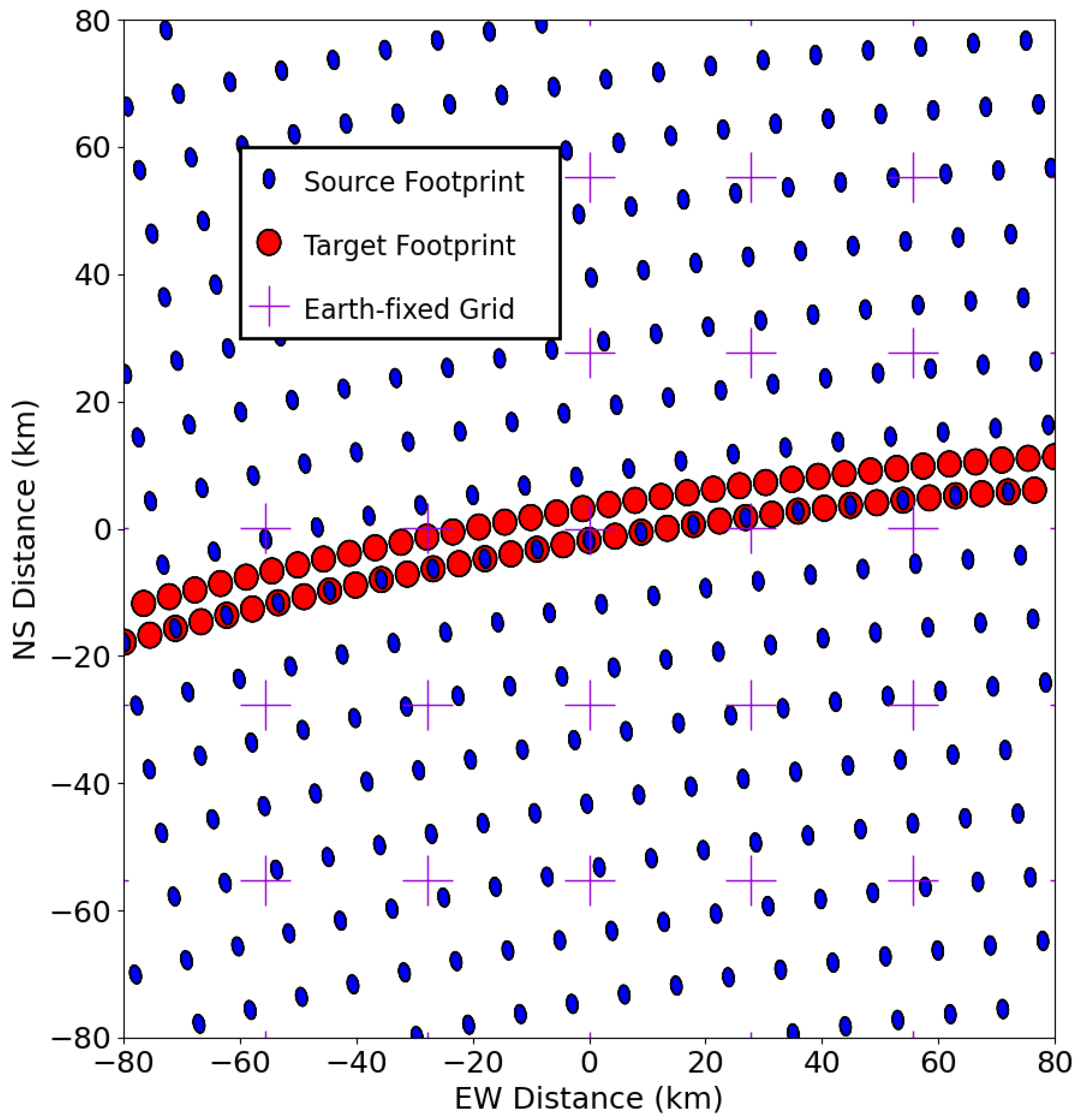
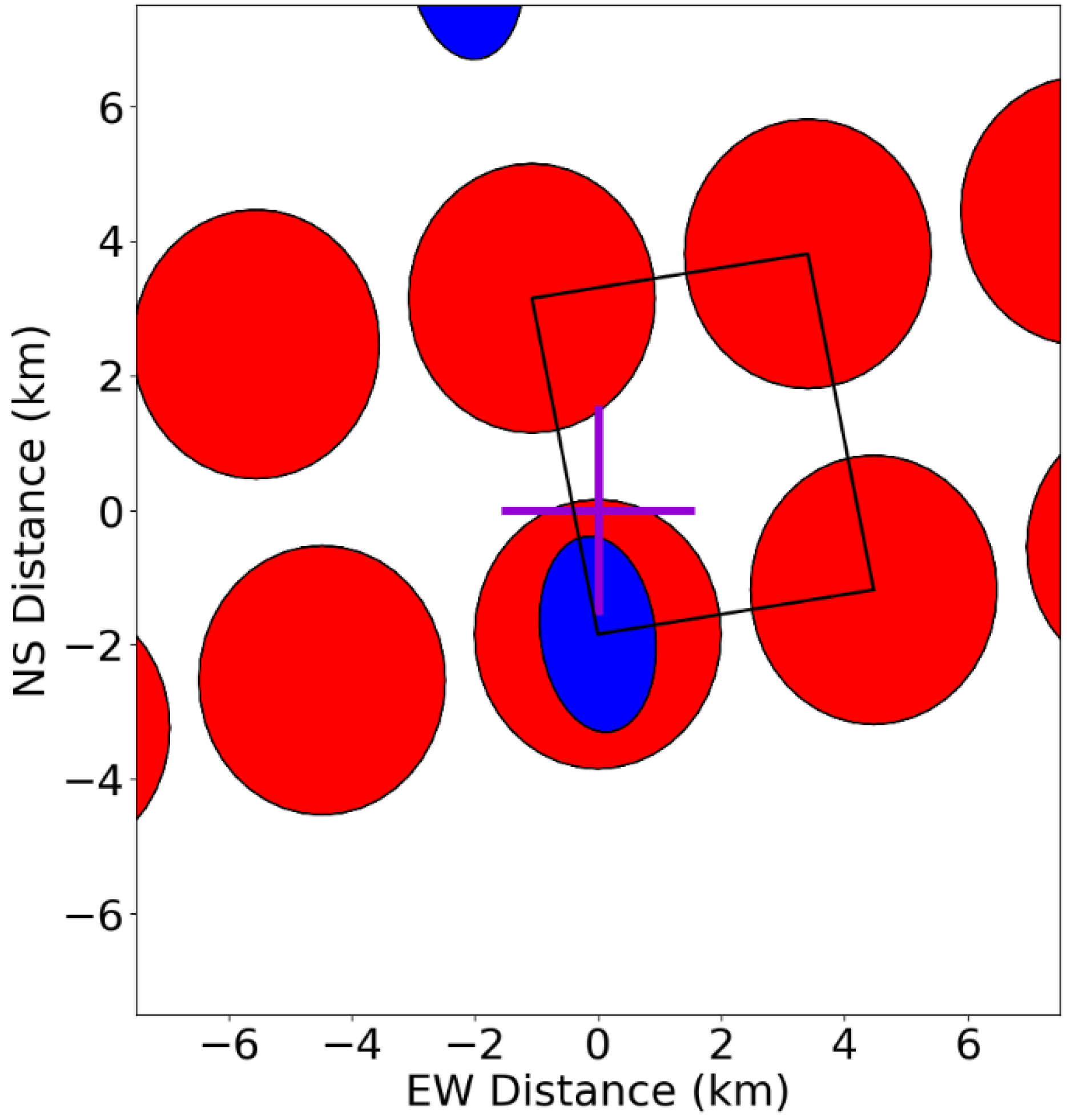
Many of the passive microwave sensors that monitor these natural emissions are conical scanners, which operate using an off-axis paraboloid antenna spinning around an Earth-directed axis. As a result, individual measurements are arranged in curved “scans” on the Earth (e.g., the blue ellipses in Figure 1). The area sampled as the satellite moves forward while orbiting defines the satellite swath. Subsequent swaths cross the equator at different longitudes as the Earth rotates. Each measurement footprint is generally elliptical, with a major axis that rotates in the Earth-fixed frame as the satellite scans. Taken together, this geometry presents a challenge for users that want to rapidly collocate satellite data with other sources of information, including maps of surface conditions (often available on a regular latitude-longitude grid), information from other satellites (which would have a different, non-aligned scan geometry), output from weather or climate models, or point-like in situ information.
The objective of the work described here is to solve the satellite geometry problem by resampling measurements from the native scan geometry to circular footprints located on a fixed Earth grid. Circular footprints enable accurate comparison between measurements made by sensors on different platforms, whose native footprints are ellipses canted at varying angles. Using a fixed Earth grid facilitates comparisons with other types of Earth system data, such as reanalysis or surface conditions, that are available on fixed grids. In this work, the resampling is performed in four steps.
The three steps use the Backus–Gilbert method [7,8], which produces estimates of radiance for an arbitrarily-shaped target footprint at an arbitrary location. This is achieved by resampling using an optimized linear combination of the source footprints. The Backus–Gilbert method is in widespread use in the microwave satellite analysis community, to collocate footprints that differ slightly in location or to match disparate footprint sizes. In most applications, the target footprint is also elliptical, which is a reasonable choice when preserving spatial resolution is desired. The goal of this work is slightly different. We want to enhance the ease of analysis for users and facilitate the use of data from different sensors as well as other data sources. This motivates our choice of Earth-fixed circular footprints.
The first step is to use the Backus–Gilbert method to calculate the weights needed to resample to a dense grid of target locations in the satellite’s scan geometry. Second, we find the locations on the grid of target locations that surround the desired Earth-fixed grid location. Third, the we use the pre-computed weights to resample the observed radiances to these locations. Finally, we use quadrilateral interpolation to interpolate these resampled radiances to the desired location on the Earth-fixed grid. As we show in Section 3 below, the interpolation procedure only results in small footprint shape distortions. This is because the interpolation is performed over distances that are less typically less than 10% of the target footprint diameter.
The choice to resample to locations in the satellite geometry as opposed to directly resampling to locations on a fixed grid is driven by computational efficiency. As discussed in more detail below, resampling to an arbitrary location requires the calculation of overlap integrals between the source and target footprints, followed by the diagonalization of moderately-sized matrices. These steps are too computationally intensive (each calculation of the resampling weights takes ~109) floating point operations) to perform for each individual target location and swath geometry in an Earth-fixed coordinated system. By performing Backus–Gilbert calculations in the swath coordinate system, the weights can be pre-computed, reducing the number of floating point operations needed to ~103).
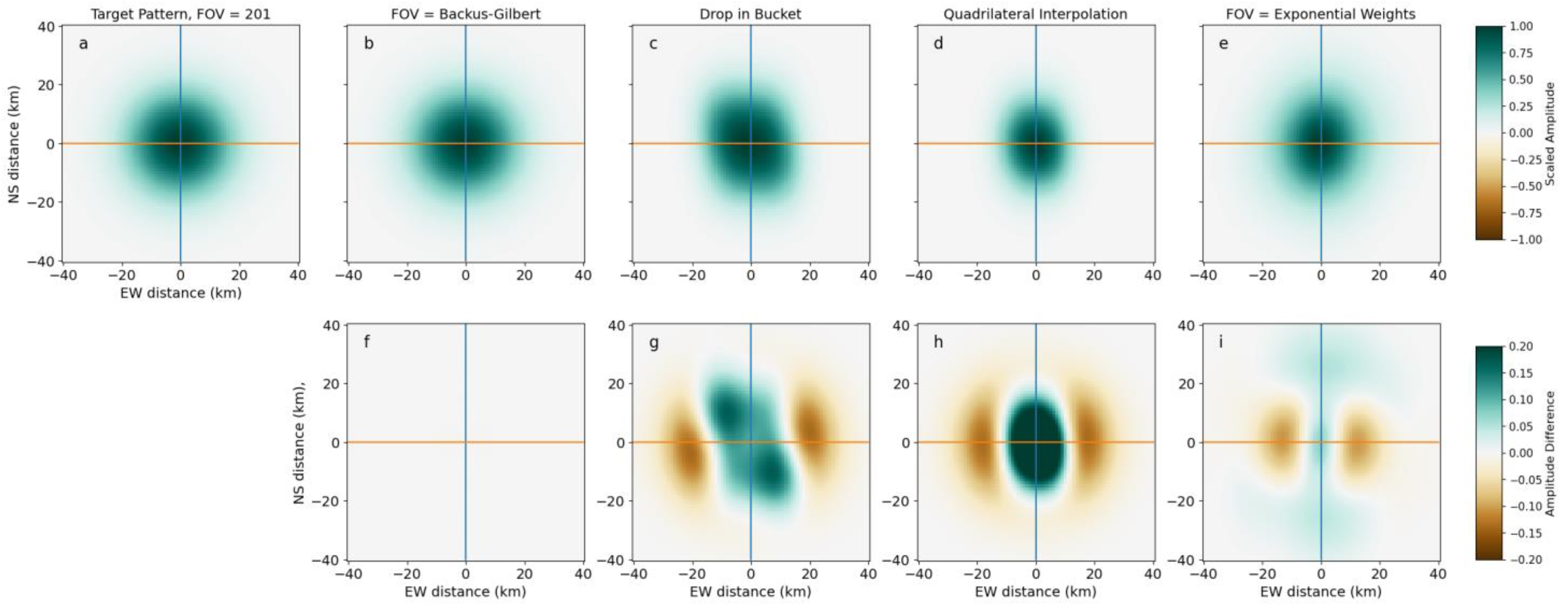
Many scientists have produced Earth-fixed datasets (either radiances or retrieved geophysical parameters) from microwave imagers. These are commonly produced using methods that result in footprint shape distortions or mislocations. For example, the 0.25 × 0.25 degree ocean parameter retrievals currently available from remote sensing systems are constructed using “drop in the bucket” averaging, where all footprints with centers located in the target grid cell are averaged together with equal weights. In Appendix A, we compare the results from the method described below with results obtained using less accurate methods.
The remainder of this paper is organized as follows: in Section 2, we describe our methodology in more detail. In Section 3, we show the results, including accuracy estimates for several types of Earth scenes, and resampled radiances from the Advanced Microwave Scanning Radiometer-2 (AMSR2). In Section 4, we conclude by discussing the practical limitations of our method when used to resample actual satellite measurements. For the remainder of the document, we will refer to microwave radiances as brightness temperatures (TBs) reported in temperature units of Kelvin (K).

2. Materials and Methods

2.1. The Backus–Gilbert Method

The goal of this work is to resample TB data records for all sensors to a common fixed Earth grid. The resampling is based on the Backus–Gilbert optimum interpolation (OI), which is an established and widely used method for sampling and gridding passive microwave satellite data [8]. This method constructs a synthetic measurement at a desired target footprint, with a given location and desired spatial shape, as a weighted sum of individual observations that overlap with that target footprint. The weights are determined to give the best possible noise reduction in the reconstructed observation.

2.2. Calculating Backus–Gilbert Weights

The resampled brightness temperature for the target footprint is approximated as a weighted sum of brightness temperatures at the source footprints:
T B , T a r = i a i T B , i
where T B , T a r is the resampled brightness temperature at the target location, and a i   and   T B , i are the weight and the brightness temperature for each source footprint, respectively. The Backus–Gilbert method provides a means to find values of the a i s that provide both a good match to the target footprint and substantial noise reduction via averaging over disparate measurements with uncorrelated radiometer noise. The coefficients a i are given by
a = V 1 v + 1 u T V 1 v u T V 1 u u
where
V = G + E β
u i = G i ρ d A
v i = G i ρ F ρ d A
G i j = G i ρ G j ρ d A
The gain functions on the Earth’s surface of the ith source footprint as a function of location ρ are given by G i ρ , and the target footprint is given by F ρ . E is the error covariance matrix of the source measurements. We assume E is diagonal with diagonal elements equal to the variance σ 2 due to radiometer noise, i.e., the measurement noise is constant and uncorrelated. β is a scaling and smoothing factor that can be adjusted to trade off the goodness of fit and noise reduction due to averaging. For the results shown here, β was chosen to be 10−5, which results in a good fit to the target footprint and a moderate amount of noise reduction. The analysis is carried out over the source footprints near enough to the target footprint so the overlap integrals v i are non-zero, to yield sets of a i s for target footprint location.
We assume that the analysis can be translated to any scan in an orbit. Thus, the analysis only needs to be carried out once for any location relative to the scan geometry. By making this assumption, we are ignoring several small effects that change the relative positions and shapes of the source footprints in different parts of the orbit. These include differences in satellite altitude, which affect the slant range and the incidence angle, and the effects of the Earth rotation relative to the movement of the measured point on the Earth due to satellite motion and the scanning process. The main effect of these will be small distortions in the shape of the target footprint so that they are no longer exactly circular or no longer exactly the targeted size. We expect these distortions to be smaller than the distortions introduced by the interpolation step. We show in Section 3 that the effect of the interpolation-induced distortions is negligible in most cases.
Under this assumption, the G matrix, which depends on the overlap between pairs of source footprints, can be precomputed, and is independent of target location. We assert normalization conditions on the source footprints so that all elements of the u vector are equal to 1.0. This means that the only calculations we need to do for each target location are to determine the elements of the v vector, which describe the overlap between the source footprints and the target footprint, and perform the matrix calculations. By far the most computationally expensive part of this process is performing the integrals numerically to calculate the target–source overlaps. This is too computationally costly to do the inversion for each combination of source footprint geometry and target footprint location.

2.3. Overview of the Method Used

Here, we propose an approximate four-step method to obtain a result for resampling to an arbitrary location. First, resampling coefficients for circular target footprints are calculated. The target footprints are both centered at the “actual” locations, i.e., the same places the satellite sensor makes measurements (the blue ellipses in Figure 1 and Figure 2), and additional “synthetic” locations located between the actual locations in both the along-scan and along-track directions. The target locations are shown by red circles in Figure 1 and Figure 2. These locations are relative to the swath geometry, so the calculation is only dependent on the relative location of the target footprint in the swath. Second, using the Earth locations of the actual satellite observations, we determine the target locations that correspond to the corners of the quadrilateral that surround the desired location. Examples of Earth locations are shown by crosses in Figure 1 and Figure 2. Third, we use pre-computed weights for the chosen four target locations to calculate an approximation of the resampled brightness temperature at the corners of the quadrilateral. Finally, a two-dimensional quadrilateral interpolation is performed to exactly place the target at the desired location.

2.4. Example of Resampling to “Synthetic” Locations

In Figure 1, we show an example of the resampling geometry for part of a swath from AMSR2 [9,10]. In this example, we insert synthetic targets between subsequent measurements in each scan, as well as synthetic scans between each real scan. Note that the number and density of the synthetic locations is arbitrary, and the location accuracy can be improved via the insertion of additional points. The number of extra locations is only limited by the memory available to store the weighting coefficients for each target location.

2.5. Choosing the Encompassing Resampled Location and the Final Interpolation

Additionally, shown in Figure 1 are the desired target locations (crosses in the figure) on a fixed Earth grid, and Figure 2 shows a “zoomed-in” version of the same locations. After Backus–Gilbert OI is performed, the next step is to find set of four resampled footprints that form the quadrilateral that encompasses the desired location, as shown in Figure 2. Once these resampled locations are determined, we can calculate the values of the resampled brightness temperatures at the vertices of the quadrilateral, which are then used to find the interpolated value at the target location. Note than in Figure 1, there are many resampled locations that are not part of any encompassing quadrilateral. The resampled values as these locations do not need to be calculated.

3. Results

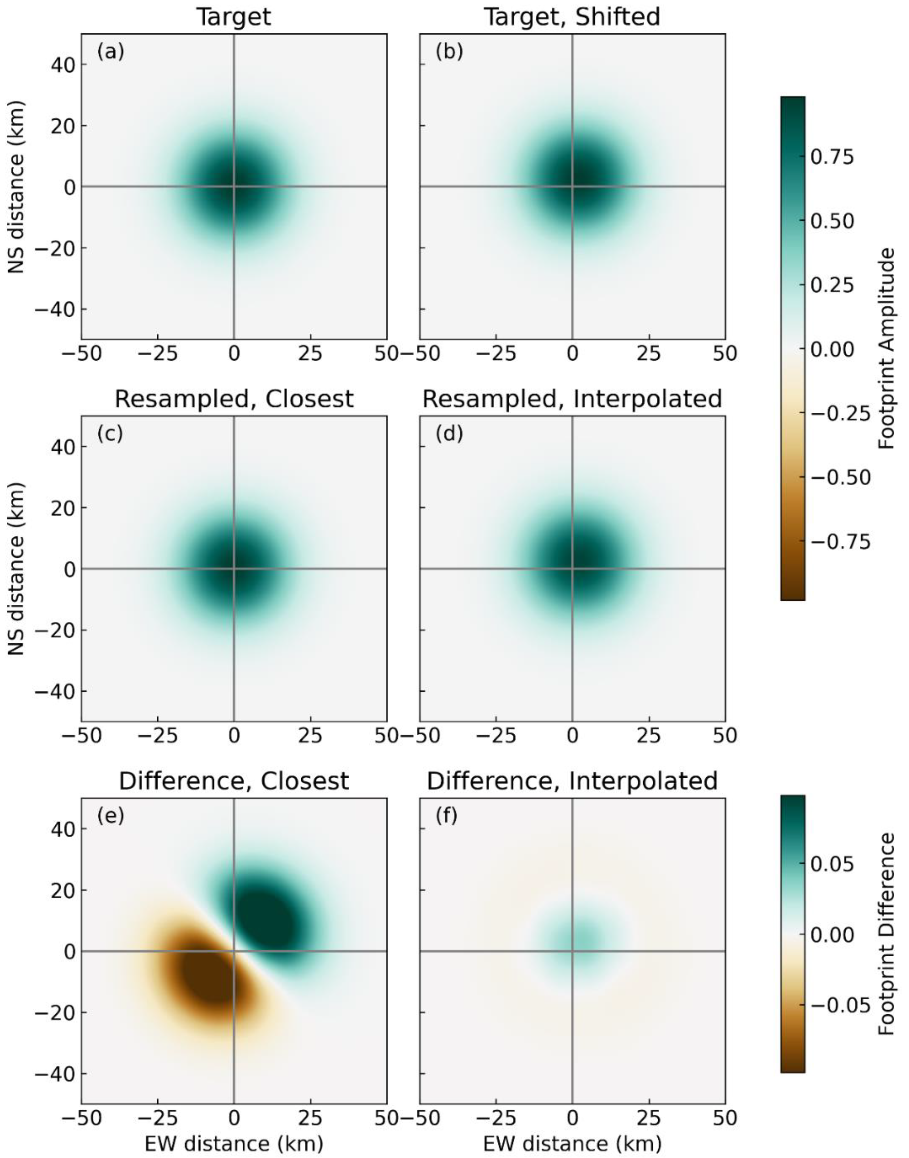
To illustrate the typical results of our methodology, we continue to use the example of AMSR2. It is important to estimate the errors introduced by our method as well as the reduction of the radiometer noise gained by the resampling procedure. We separate the resampling error into two parts: the error due to the difference between the resampled footprint and the ideal target footprint, and the error introduced by the location of the resampled footprint relative to the location of the target as shown in Equation (7).
G r e s a m p ( ρ δ ρ ) G t a r g e t ( ρ ) = G r e s a m p ( ρ ) G t a r g e t ( ρ ) + G r e s a m p ( ρ δ ρ ) G r e s a m p ( ρ )
where G r e s a m p ( ρ ) is the amplitude of the resampled footprint at location r, G t a r g e t ( ρ ) is the amplitude of the target footprint, and δ ρ is the location difference between the target and resampled footprints. Analysis of the location difference term provides motivation for the interpolation step in our method.
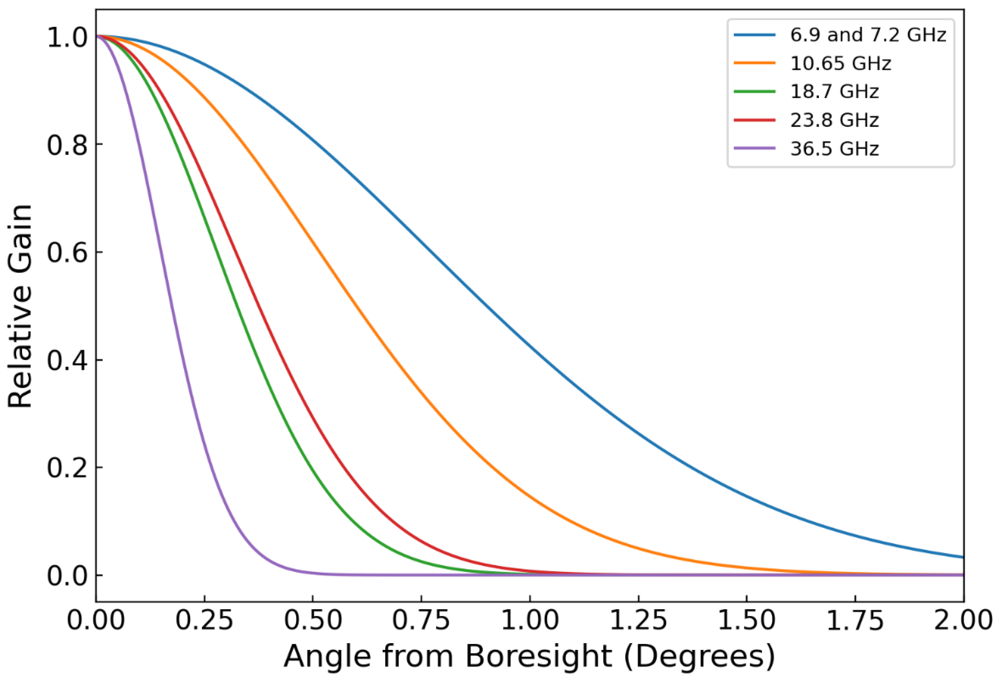
As discussed earlier, the first step is to calculate the Backus–Gilbert weights for each frequency and target footprint. For the source footprints, we start with a simplified, radially symmetric antenna gain function:
G ( θ ) = a f + b f e c f θ + e d f θ 2
The values for the coefficient for each channel and the resulting full-width at half maximum (FWHM) are given in Table 1. Because the coefficient b is much smaller than one, these gain functions are very close to a Gaussian. The actual gain functions are not exactly radially symmetric, and have small side-lobes outside of the first zero. Including these in the calculation would add needless complication to our heuristic treatment presented here, but they could be included if they are known with sufficient accuracy. The gain as a function of off-boresight angle is plotted in Figure 3.
These gain functions are converted to footprints on the Earth’s surface by projecting the gain function onto the surface using a nominal Earth incidence angle of 55 degrees, resulting in footprints that are approximately elliptical Gaussians, with the major axis aligned along the azimuth angle. The resulting footprints are also slightly elongated in the minor-axis direction because of the non-zero integration time for each measurement. The 3-dB size of each footprint on the Earth’s surface is presented in Table 1. For 10.65 GHz channels and above, we define target functions that are to be circular Gaussian functions with a FWHM diameter of 30 km. For the 6.9 and 7.2 GHz channels, larger target footprints with a diameter of 70 km are required. These are discussed in Appendix B.

3.1. Examples of Resampled Footprint Shape and Error Estimates

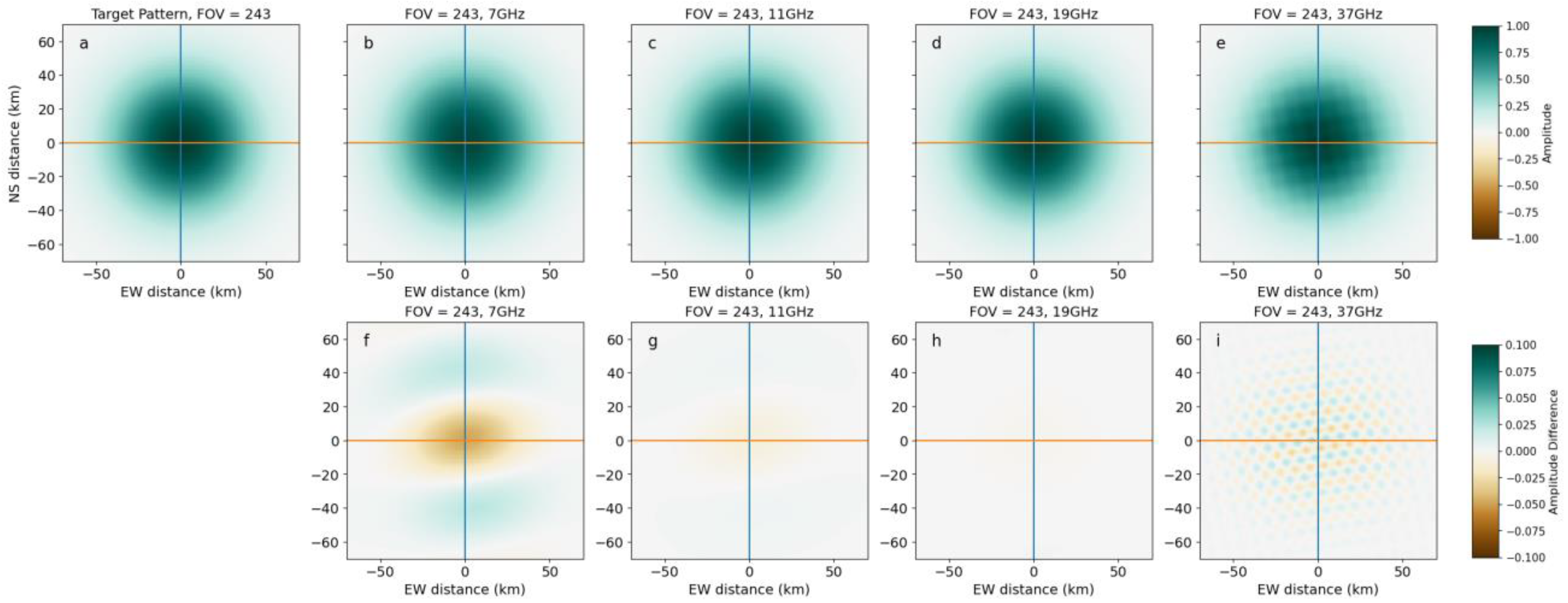
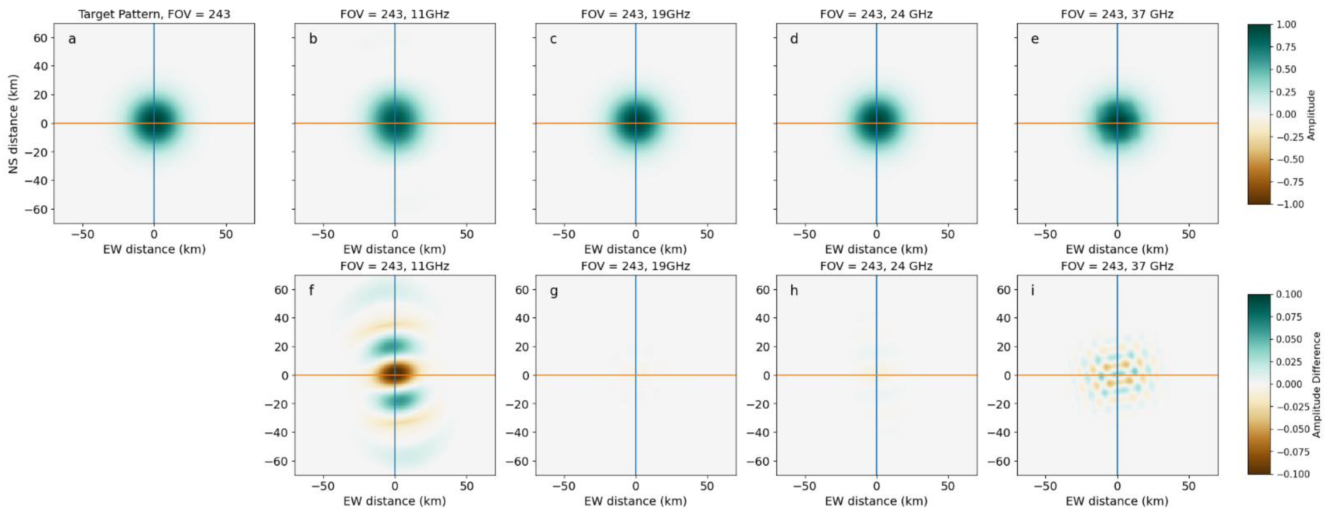
In this section, we show comparisons between the desired target footprints and the resampled footprints for several locations in the swath for the frequencies of interest. In Figure 4, we provide an example from near the center of the AMSR2 swath with a target diameter of 30 km. The resampled pattern for 19 GHz (c) and 24 GHz (d) are nearly perfect, with the difference between the target and resampled patterns being nearly zero (g and h). At 37 GHz, the source footprints are slightly too small to accurately match the target pattern, resulting in the high-frequency spatial variability seen in (i). For 11 GHz, the major axis of the source pattern (42 km) is larger than the diameter of target pattern, leading to distortions along this axis, as seen in (f). If the observed scene has large gradients along this axis, substantial errors could result (see Figure 7c). Accurate sampling of the 11 GHz channel would require a larger target footprint, but a 30 km resampled product may still be useful for some applications, despite these distortions. Because each of the sampled patterns are a combination of a number of actual observations, the resampling procedure reduces the contributions of random sensor noise. We do not expect further reduction of noise when we perform the final interpolation step, because the noise in neighboring resampled footprints is highly correlated as they are constructed from sets of native observations with many common elements.
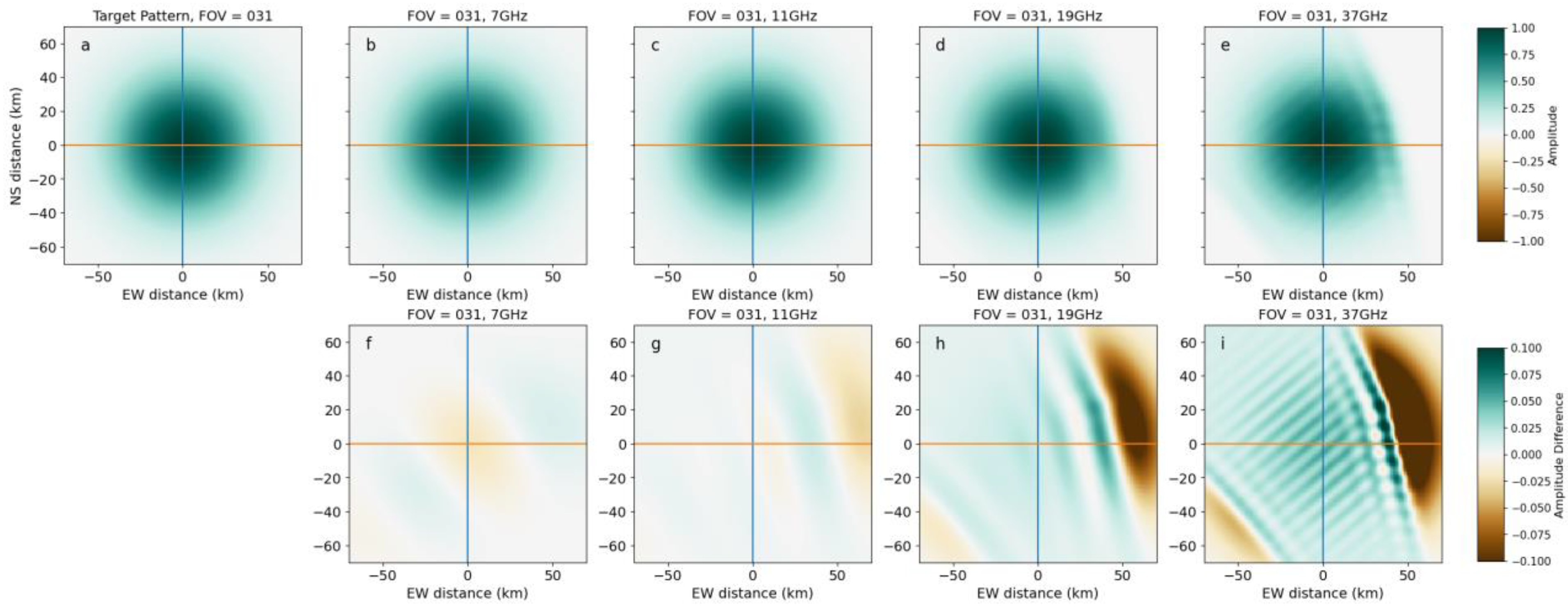
Other locations in the swath show different results. In Figure 5, we display results analogous to Figure 4 for a location close to the swath edge. In this case, the results for 37 GHz (e and i) are substantially degraded. Because of the relatively small footprint size for 37 GHz, there is no measurement weight available to provide any weight on the right side of the target footprint, leading to large errors. The other frequencies with their larger footprints, are not substantially degraded until the target footprint is even closer to the swath edge than the example location shown here.
The effect of the differences between the ideal target footprint and the resampled footprints will depend on the scene being viewed. Because we have forced the sum of the a i s to be 1.0, there will be no error for a scene wherein the radiance is constant, independent of position. As the spatial variability increases, the footprint differences become more important. To demonstrate the dependence of the error on scene properties, we use several idealized versions of real Earth scenes in addition to representative Earth scenes (Figure 6 and Figure 7). For microwave frequencies used in microwave imagers, the atmosphere is fairly transparent, and much of the observed radiance is determined by surface properties such as temperature and emissivity. The emissivity difference between dry land and water is typically large, leading to brightness temperature differences as large as 100 K, particularly for horizontally polarized (h-pol) radiation. Therefore, some of the most challenging scenes for microwave imagers are those that mix land and water. Over the open ocean, brightness temperatures are determined by surface wind, sea surface temperature, and atmospheric moisture, which all vary much more smoothly.
We choose to investigate three representative types of Earth scenes as well as two idealized scenes. The Earth scenes are (1) from a location in the Canadian Shield with a large number of lakes, (2) from a simpler land area with some lakes and rivers along the Missouri River, and (3) from a complex coastline along the New England coast (Figure 6a–c). We also consider two idealized scenes: (1) a linear coastline at randomly chosen angles, and (2) a land fraction gradient, also in random directions (Figure 6d,e). The land fraction gradient can be considered a proxy for smoothly varying scenes that might be encountered over the rain- and ice-free ocean. In Figure 6, we show representative land fraction maps from each set of scenes. For Earth-derived scenes, the central latitude and longitude are given in Table 2. The center of the actual scenes used in our calculations are randomized locations in the regions shown in Figure 6. These are taken from a box extending ±1 degree in both latitude and longitude from the central location. For the coastline, the scene is rejected if the land fraction averaged over the target footprint is <0.15 or >0.85. This is to prevent contributions from scenes that are not truly coastal scenes. The idealized linear coastline is constructed using a random direction for the orientation of the coastline, and then is displaced randomly ±10 km in both the N-S and E-W directions. These displacements and rotations are added to avoid unrealistic agreements between the target and resampled values because of the symmetry in differences between them. For the gradient scene, the orientation of the gradient is varied randomly. For each type of scene, the difference between the brightness temperature calculated over the target footprint and the resampled footprint is tabulated over 1000 random scenes. We use the root mean square of these differences as an estimated error.
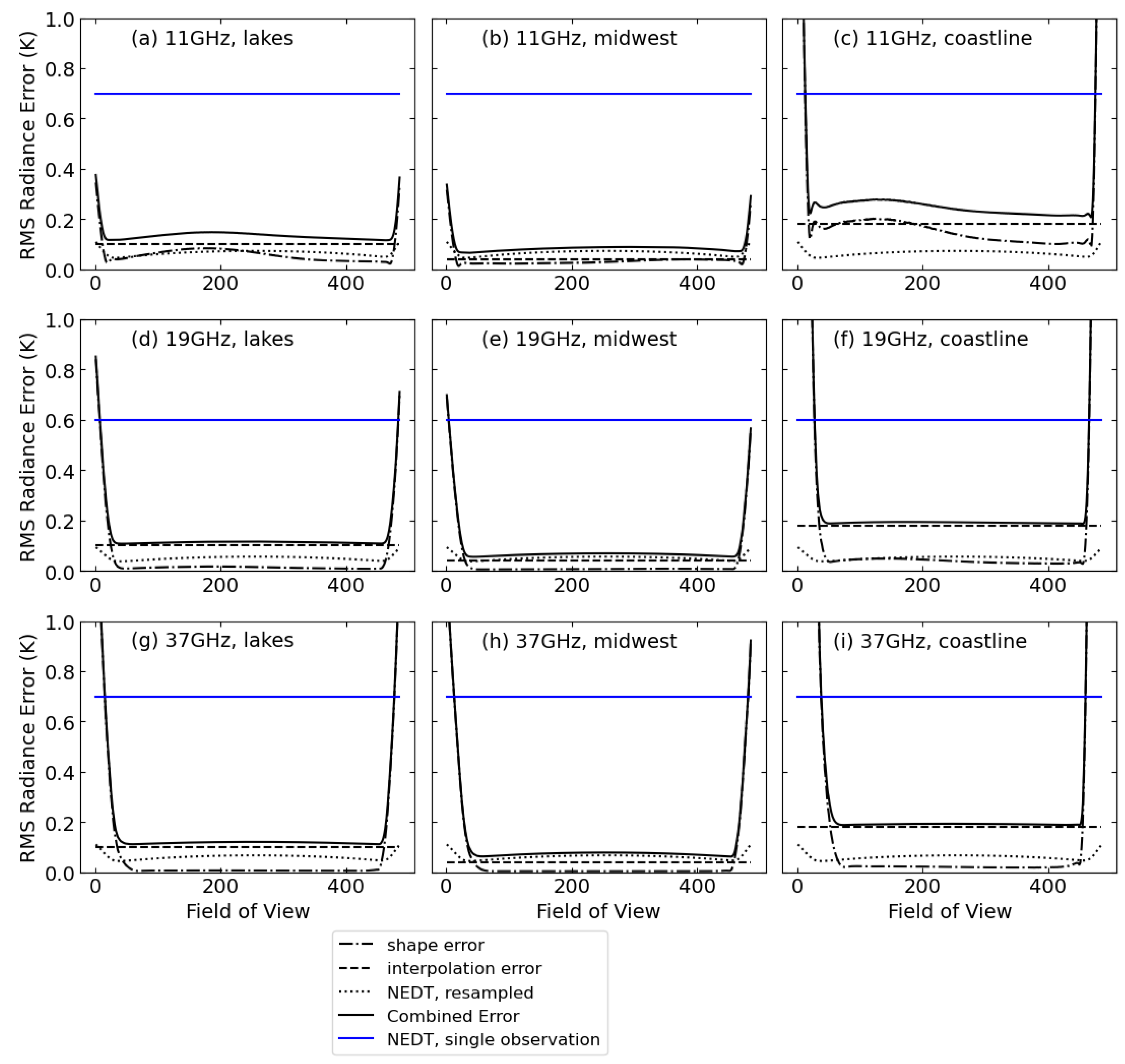
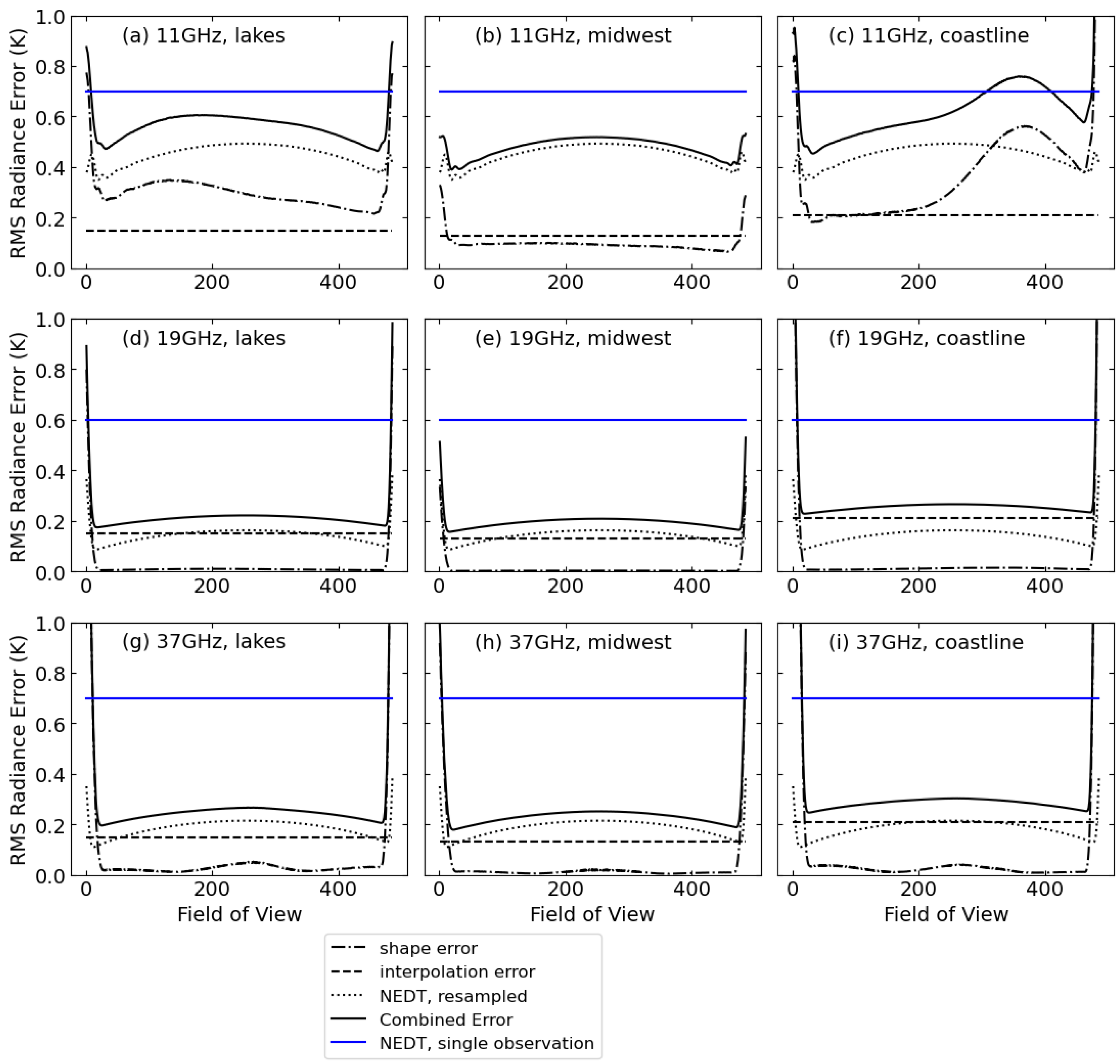
The estimated error for different types of scenes changes as the location in the swath varies (Figure 7). Near the edges of the swath, the lack of available weight to fill in the edge of the target footprint becomes important, and the estimated errors increase. The errors for the 11 GHz channel are larger, reflecting the large differences between the resampled footprint and the 30 km target footprint. This is especially evident for the coastline scene for the part of the swath where the land–ocean gradient is aligned with the footprint axis. For the 19 and 37 GHz channels, the shape-induced error is much smaller than the errors from radiometer noise, which are typically on the order of tenths of K.
The above analysis was repeated for 70 km footprints. For the larger footprints, we included all AMSR2 frequencies from 6.9 GHz to 37 GHz. The 70 km footprints were the smallest footprints that resulted in adequate performance for the larger 6.9 and 7.2 GHz source footprints. The results of this analysis are presented in Appendix B.

3.2. Errors Due to Mislocation

The above results show the performance of the method when a resampled footprint is exactly collocated with the target location. In practice, this rarely occurs. A second source of error in resampling is due to the difference between the location of the resampled footprint and the location of the grid-located target. For the number of synthetic footprints used in this example, the typical distance between the target location and the closest resampled footprint is typically in the range of 1 to 3 km. We wish to investigate the estimated error if we use the closest resampled footprint, i.e., if we skip the interpolation step (step 2 in our method). Because the target footprint shapes are fairly well-matched at all frequencies (as least far from the swath edge), this type of error is largely independent of frequency. In Figure 8, we show the effects of a mislocation error due to a 2.8 km diagonal shift in brightness temperature differences, which is typical of the larger location error in our example geometry. Panel (e) shows the difference between the resampled footprint closest to the target (c) and the shifted target footprint (b). The difference is substantial, and will lead to large errors in scenes with large derivatives in the direction aligned with the mislocation vector. For the example plotted in Figure 8, a coastline that is oriented southeast to northwest would result in large errors.
We use a simulation similar to that described in Section 3.2 (Figure 6 and Figure 7) to quantify the effects of location errors on both representative and idealized Earth scenes. In this version of the simulation, target footprints are randomly located in the quadrilateral defined by the four adjacent resampled footprints in the along-scan and cross-scan directions. An example of such a quadrilateral is shown in Figure 2. The top row in Table 3 shows the root-mean-square (RMS) average of simulated location errors for 1000 simulated target locations. Results are shown for each of the five scene types. In each case, the differences between the randomly located target footprint and the closest resampled footprint were evaluated. The simulated errors for the lakes, coastline, and edge scenes are substantially larger than the typical noise equivalent delta equivalent temperature (NEDT) for satellite-borne imaging radiometers, which range from 0.4–0.7 K.
There are two ways to reduce the mislocation error. First, we could calculate the resampling weights in a finer synthetic grid so that the distance between the resampled and target footprint is reduced. The disadvantage of this approach is that more memory is required to store the resampling weight arrays, which could reduce the portability of the algorithm. A second approach is to use two-dimensional interpolation to locate the target footprint at the desired location, but with a small amount of additional shape mismatch error. The disadvantage of this approach is that it is more computationally expensive, because the resampled radiances need to calculated for the four synthetic footprint locations that encompass the target location. An example of one of these quadrilaterals is shown in Figure 2. Here, we investigate this second approach, which ultimately forms the basis for “Step 2” in our methodology. We use a quadrilateral interpolation technique that transforms the quadrilateral to a square via a linear transformation. After the transformation, bilinear interpolation can be used. This technique requires that the original quadrilateral to be convex. Fortunately, all quadrilaterals formed by adjacent sets of footprint locations are close to being parallelograms, and thus are convex. Figure 8f shows the difference between the interpolated footprint and the target footprint. The results are much improved relative to the “closest” result in Figure 8e. The “bullseye” shape of the difference in Figure 8f indicates that the resampled footprint is slightly larger than the target footprint due to the interpolation procedure.
The second row of Table 3 shows the results after the interpolation step. All results are improved relative to the “closest” case. The scenes with the largest errors (the coastline and edges scenes) are improved by more than a factor of 10. Importantly, all the simulated errors are now less than the typical NEDTs for satellite-borne radiometers.

3.3. Caveats and Limitations

In the treatment above, we have assumed that the geolocation accuracy of the satellite data is perfect. For actual microwave satellite data, there are possible geolocation errors in the range of 1–2 km [11], which would also contribute to the radiance errors for complex scenes. The additional sources of data indicate that further improvements to the algorithm presented above are not useful in practice, since it is likely that the geolocation errors will dominate the error budget.
A second assumption is that the native footprints can be accurately approximated using the near-Gaussian functions in Equation (8). The actual footprints will have additional features such as sidelobes that will modify the shape of the resampled footprint. If detailed and accurate antenna gain patterns were available, these effects could be ameliorated by our method, but often such detailed information is not provided by the instrument teams, and if available, are based on ground-based results from antenna measurements performed in the near-field, which may not accurately represent on-orbit behavior.

3.4. Example Output Using AMSR2 Measurements

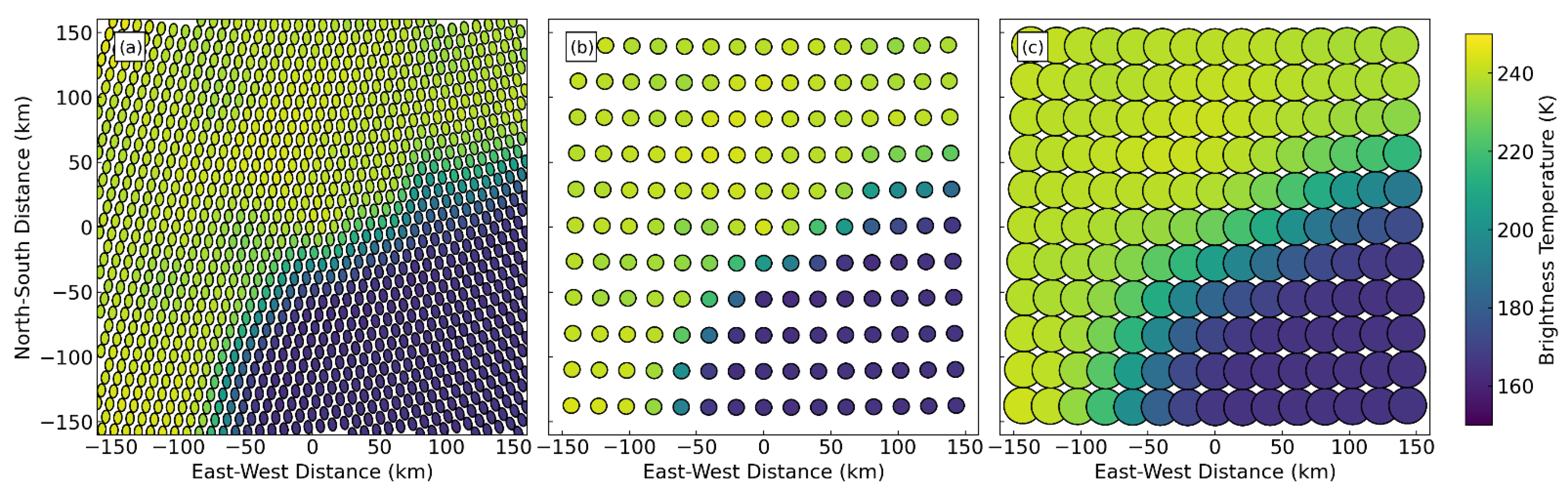
We have used the described method to resample AMSR2 radiances to both 30 km and 70 km circulator footprints onto a regular latitude-longitude grid. In Figure 9, we show an example of the regular latitude–longitude grid for a location centered at 44 N, 74 E on the coast of Maine. The elliptical footprints in panel (a) are resampled and interpolated to the 30 km and 70 km circular footprints in panels (b and c). Note that the 70 km results are smoother than the 30 km results due to the loss of spatial resolution caused by resampling to the larger footprints.

4. Discussion

We have presented a reasonably accurate method for resampling radiance observations from microwave imagers to circular footprints at arbitrary locations. In the case presented, we resample to a fixed earth grid to facilitate collocation with data from other satellites, other sources of Earth observations, and numerical Earth simulation output. We expect our results will be most useful for complex scenes, such as near coastlines, regions with numerous lakes, and near the sea-ice edge. For these complex scenes, simpler methods of producing gridded data (such as “drop in the bucket” averaging) will lead to substantial errors.

Author Contributions

Conceptualization, F.W. and C.M.; methodology, C.M., F.W. and A.M.; software, C.M. and A.M.; validation, C.M. and A.M.; writing—original draft preparation, C.M.; writing—review and editing, A.M.; visualization, C.M. and A.M.; funding acquisition, C.M. All authors have read and agreed to the published version of the manuscript.

Funding

This research was funded by the NASA’s Earth Science Data Systems program, project ACCESS19-0031.

Data Availability Statement

This study uses a number of input datasets listed here: AMSR2 L1A: ERA-5 (atmospheric and surface ancillary data from reanalysis): https://www.ecmwf.int/en/forecasts/dataset/ecmwf-reanalysis-v5 (accessed on 1 July 2022. IMERG: (satellite-derived global rain rates) https://gpm.nasa.gov/data/imerg (accessed on 4 August 2022). The resampled radiances from AMSR2 are freely available on the Remote Sensing System website: https://www.remss.com/measurements/earth-gridded-microwave-radiance-data-collection/ (accessed on 23 March 2022).

Conflicts of Interest

The authors declare no conflict of interest.

Appendix A

In this appendix, we compare results between the method discussed in the main text and other methods that could be used to generate Earth-gridded data from polar-orbiting microwave imagers. In these alternative methods, the target footprint is often not explicitly defined, and the purpose is to generate a map visualization of measured radiances or retrieved geophysical parameters. We compare three alternative methods.
Drop-in-the-bucket averaging. Within this method, all the radiances corresponding to all footprints whose center is inside the target latitude/longitude rectangle are averaged with equal weight.
Interpolation of near-neighbors. Within this method, we use quadrilateral interpolation to interpolate the radiances of the four near-neighbor actual measurements that surround the target location.
Exponential Weighting. Within this method, all footprints within a specified distance are included, with a weight that decays exponentially with distance as the distance from the target location increases. We chose the length scale of the exponential decay to minimize the difference between the resampled footprint and the target footprint near the center of the pattern. For this method, we normalize the exponential weights so that they total 1.0.
Figure A1. Comparison of the 30 km target pattern (a) and resampled patterns for 19 GHz (be) for resample patterns constructed using the Backus–Gilbert, drop-in-the-bucket, near-neighbor interpolation, and exponential weighting, respectively. This example is taken from the center of the swath. Subplots (fi) show the difference between the target pattern and resampled patterns for the various methods.
Remotesensing 15 05047 g0a1
Figure A1 summarizes the comparison for 19 GHz resampled footprints. The Backus–Gilbert method reproduces the target footprints almost exactly, as was also shown in Figure 4. All other methods show substantial differences between the target footprint and the resampled footprints. This is not surprising, since these methods were not designed to reproduce a specific target footprint. Using the same methods as described in the main text, we estimate the brightness temperature errors caused by the shape mismatches shown in Figure A1 (see Table A1). Note that the Backus–Gilbert column in Table A1 is identical to the second row of Table 3 in the main text. In all cases, the alternative methods show much larger errors, especially for the coastline and edge cases.
Table A1. Estimated brightness temperature errors caused by footprint mismatch.
Backus–GilbertDrop-in-the-BucketInterpolation of
Nearest Neighbors
Exponential Weighting
Lakes0.151.2862.9970.631
Farmland0.130.5371.0940.163
Coastline0.211.4014.3620.767
Edges0.212.7296.2251.229
Gradient0.0010.010.0720.079

Appendix B

In this appendix, we show similar results to those discussed in the main text for 70 km diameter target footprints. These larger footprints are needed for the lower-frequency 6.9 and 7.2 GHz channels for AMSR2.
Figure A2. Similar to Figure 4, except for 70 km diameter target footprints. The figure shows then target pattern (a) and resampled patterns (be) for 7, 11 19, and 37 GHz AMSR2 channels, respectively. This example is taken from the center of the swath. Subplots (fi) show the difference between the target pattern and resampled patterns for 7, 11 19, and 37 GHz AMSR2 channels, respectively. For the larger footprint, the match at 11 GHz is nearly perfect. At 7 GHz (6.9 and 7.3 GHz), there are differences analogous to the differences for the 30 km target footprints at 11 GHz, caused by the target footprint being slightly smaller than the major axis of the source footprints.
Remotesensing 15 05047 g0a2
Figure A3. Similar to Figure 5, except for 70 km diameter target footprint and for FOV number 31. The figure shows then target pattern (a) and resampled patterns (be) for 7, 11 19, and 37 GHz AMSR2 channels, respectively. This example is taken from the center of the swath. Subplots (fi) show the difference between the target pattern and resampled patterns for 7, 11 19, and 37 GHz AMSR2 channels, respectively. Because of the larger target footprint, large errors extend further in from the edges of the swath than they did for the 30 km footprints.
Remotesensing 15 05047 g0a3
Figure A4. Similar to Figure 7, except for 70 km footprints. Estimated radiance errors as a function of the resampled field of view (FOV) in the satellite scan. FOVs 1 and 485 refer to the left and right swath edges, with FOV 243 at the center of the scan. Each columncorresponds to three realistic scene types (lakes (panels a, d, g), midwest (panels b, e, h), and coastline (panels c, f, i)), and each row corresponds to a measurement frequency (11 (panels a–c), 19 (panels d–f), and 37 GHz (panels g–i)) In each panel, the solid blue line shows the noise equivalent delta temperature (NEDT) for single AMSR2 observations. The solid black line shows in the combined error from shape error, interpolation error, and resampled NEDT. The other black lines show each of these contributions separately. In all cases, the NEDT is reduced by the averaging inherent in the resampling process. This reduction is larger for the 70 km footprints than it is for the 30 km footprints, because more averaging is performed. For all frequencies and scenes, the errors become large near the swath edge. Because the target footprint is larger, the region of large errors extends further from the edge of the swath than it does for the 30 km footprints.
Remotesensing 15 05047 g0a4

References

  1. Ulaby, F.T.; Moore, R.K.; Fung, A.K. Microwave Remote Sensing: Active and Passive; Ulaby, F.T., Ed.; Remote Sensing: A Series of Advanced Level Textbooks and Reference Works; Artech House: Norwood, MA, USA, 1981; Volume I: Microwave Remote Sensing Fundamentals and Radiometry, ISBN 0-89006-190-4. [Google Scholar]
  2. Wentz, F.J. A Well Calibrated Ocean Algorithm for Special Sensor Microwave/Imager. J. Geophys. Res. 1997, 102, 8703–8718. [Google Scholar] [CrossRef]
  3. Prigent, C.; Rossow, W.B.; Matthews, E. Microwave Land Surface Emissivities Estimated from SSM/I Observations. J. Geophys. Res. 1997, 102, 21867–21890. [Google Scholar] [CrossRef]
  4. Karbou, F.; Prigent, C.; Eymard, L.; Pardo-Carrion, J.R. Microwave Land Emissivity Calculations Using AMSU Measurements. IEEE Trans. Geosci. Remote Sens. 2005, 43, 948–959. [Google Scholar] [CrossRef]
  5. Wen, J.; Su, Z.; Ma, Y. Determination of Land Surface Temperature and Soil Moisture from Tropical Rainfall Measuring Mission/Microwave Imager Remote Sensing Data. J. Geophys. Res. 2003, 108, ACL 2–1–ACL 2–10. [Google Scholar] [CrossRef]
  6. Njoku, E.G.; Jackson, T.J.; Lakshmi, V.; Chan, T.K.; Nghiem, S.V. Soil Moisture Retrieval from AMSR-E. IEEE Trans. Geosci. Remote Sens. 2003, 41, 215–229. [Google Scholar] [CrossRef]
  7. Backus, G.E.; Gilbert, F. Uniqueness in the Inversion of Inaccurate Gross Earth Data. Philos. Trans. R. Soc. Lond. A 1970, 266, 123–192. [Google Scholar] [CrossRef]
  8. Poe, G.A. Optimum Interpolation of Imaging Microwave Radiometer Data. IEEE Trans. Geosci. Remote Sens. 1990, 28, 800–810. [Google Scholar] [CrossRef]
  9. Takashi, M.; Kazumori, M.; Aonashi, K.; Shibata, A.; Cho, K.; Kelly, R.E.; Koike, T. Descriptions of GCOM-W1 AMSR2; Japan Aerospace Exploration Agency—Earth Observation Research Center: Hatoyama, Japan, 2013. [Google Scholar]
  10. Imaoka, K.; Kachi, M.; Kasahara, M.; Nakagawa, K.; Oki, T. Instrument Performance and Calibration of AMSR-E and AMSR2. Int. Arch. Photogramm. Remote Sens. Spat. Inf. Sci. 2010, XXXVIII Pt 8, 13–16. [Google Scholar]
  11. Wentz, F.J.; Draper, D. On-Orbit Absolute Calibration of the Global Precipitation Measurement Microwave Imager. J. Atmos. Ocean. Technol. 2016, 33, 1393–1412. [Google Scholar] [CrossRef]
Figure 1. Example of the scan and resampling geometry for the Earth remote-sensing instrument AMSR2. The blue ellipses show the locations of the measured or “source” footprints, i.e., the locations where the satellite makes measurements. At the location shown (near the Equator), the satellite is approximately moving south to north, so each tilted horizontal row represents part of each conical scan. The red circles represent the locations of the target footprints. Some of the target footprints are collocated with the source footprints. Others are located at “synthetic” locations, either between the source locations in the along-scan direction, or on a synthetic scan located between two source scans in the along-track direction. In this example, we add additional “synthetic” locations centered between subsequent measurements in each scan, as well as an additional “synthetic” scan centered between subsequent actual scans. The ellipses and red circles are only used to show locations. The actual footprints are 20–50 times larger. We also show the grid centers of a regular 0.25° × 0.25° Earth-fixed latitude/longitude grid using purple crosses.
Remotesensing 15 05047 g001
Figure 2. A version of Figure 1 with expanded axes showing an example of the quadrilateral over which the interpolation is performed. The desired target location is shown by the purple cross. The blue ellipse represented a source footprint, and the red circles represent the resampled target locations in the scan geometry. The radiances for resampled footprints at the corners of the quadrilateral are used to calculate an interpolated value at the target location. Note that the actual footprints are ~10× than the footprints shown.
Remotesensing 15 05047 g002
Figure 3. Radial antenna gain function for AMSR2 for each channel used in this work.
Remotesensing 15 05047 g003
Figure 4. Comparison of the 30 km target pattern (a) and resampled patterns (be) for 11,19,24, and 37 GHz AMSR2 channels, respectively. This example is taken from the center of the swath. Subplots (fi) show the difference between the target pattern and resampled patterns for 11, 19, 24, and 37 GHz AMSR2 channels, respectively. FOV refers to the field-of-view index across each resampled scan. FOVs 1 and 485 refer to the left and right swath edges, with FOV 243 at the center of the scan.
Remotesensing 15 05047 g004
Figure 5. This figure is the same as Figure 4, except for a location (FOV = 11) near the edge of the swath. Subplots (ai) show the difference between the target pattern and resampled patterns for 11, 19, 24, and 37 GHz AMSR2 channels, respectively. FOV refers to the field-of-view index across each resampled scan.
Remotesensing 15 05047 g005
Figure 6. Typical sample scenes used in our study. The “lakes”, “midwest” and “coastline” scenes (ac) are derived from a high-resolution land/water mask. The linear and gradient scenes (d,e) are idealized scenes. In both (d,e), the orientation of the feature is varied randomly, and in (d), it is translated randomly in both the x and y directions by ±10 km. For the “coastline” and “linear” scenes, the results contribute to the final statistics if the weighted land fraction for the target scene is between 0.15 and 0.85. The excluded scenes that have too much land or ocean to be representative of these types of scenes. The red circles show the size of the 3 dB contour of the 30 km footprints.
Remotesensing 15 05047 g006
Figure 7. Estimated radiance errors as a function of the resampled field of view (FOV) in the satellite scan. FOVs 1 and 485 refer to the left and right swath edges, with FOV 243 at the center of the scan. The results plotted here are from the lower scan of red circles in Figure 1, i.e., the scan that contains the actual measurement (blue) footprints within the red ones. The results only vary by a few percent for the other synthetic scan in Figure 1. Each columncorresponds to three realistic scene types (lakes (panels a, d, g), midwest (panels b, e, h), and coastline (panels c, f, i)), and each row corresponds to a measurement frequency (11 (panels ac), 19 (panels df), and 37 GHz (panels gi)) In each panel, the solid blue line shows the noise equivalent delta temperature (NEDT) for single AMSR2 observations. The solid black line shows in the combined error from shape error, interpolation error, and resampled NEDT. The other black lines show each of these contributions separately. In all cases, the NEDT is reduced by the averaging inherent in the resampling process. This effect is less dramatic for the 11 GHz channel, where the footprint is slightly smaller than the major axis for native footprints; thus, some “sharpening” occurs, which tends to increase noise. For all frequencies and scenes, the errors become large near the swath edge. The bump in the coastline error near FOV = 380 corresponds to a condition when the land-ocean gradient in the coastline scene is close to co-linear with the largest spatial variation in the difference between the resampled and target footprints (Figure 4f and Figure 5f).
Remotesensing 15 05047 g007
Figure 8. Explanation of the effects of a location error, and the results after using interpolation to ameliorate the error. Panel (a) shows the target footprint at the location of the resampled footprint, and panel (b) shows the same footprint shifted diagonally up and to the right by 2.8 km. Panel (c) shows the resampled footprint closest to the shifted location, which is located at the origin, the same as the target footprint in (a). Panel (d) shows an interpolated footprint constructed from a linear combination of four resampled footprints that surround the shifted location. Panel (e) shows the difference between the shifted target footprint (b) and the closest resampled footprint (c). Note that the color bar for panels e and f covers a range 10 times smaller than the color bar range of panels (ad). Panel (f) shows the difference between the shifted target footprint (b) and the interpolated resampled footprint in (d).
Remotesensing 15 05047 g008
Figure 9. Example of native radiance and resampled radiances for AMSR2, revolution 29,921, from 1 January 2018. (a) shows the locations of the native footprints. (b) shows the locations and brightness temperatures of the 30 km footprints, and (c) shows the locations and brightness temperatures of the 70 km footprints. In all three panels, the actual footprints are ~5 times larger than those shown.
Remotesensing 15 05047 g009
Table 1. AMSR2 antenna pattern parameters.
Frequency (GHz)Channel Name a f b f c f d f FWHM
(°)
Size on Earth (km)
6.9 and 7.274.343 ×·10−66.892·×·10−40.5030.6511.862 × 35
10.65112.096·×·10−64.059·×·10−40.7921.9261.242 × 24
18.7191.890·×·10−63.727·×·10−41.6196.5630.6522 × 14
23.8241.623·×·10−67.251·×·10−41.8434.9290.7526 × 15
36.5370.725·×·10−63.051×··10−42.34022.660.3512 × 7
For the remainder of the manuscript, we will refer to the various frequencies using the “channel names” shown in Table 1, for brevity.
Table 2. Central locations of representative earth scenes.
NameLatitudeLongitude
lakes53.0 N65.0 W
midwest45.2 N98.0 W
coastline43.5 N70.0 W
Table 3. Estimated radiance error (K) due to simulated location errors.
LakesMidwestCoastlineEdgesGradient
closest0.950.293.113.780.68
interpolated0.150.130.210.210.001
Disclaimer/Publisher’s Note: The statements, opinions and data contained in all publications are solely those of the individual author(s) and contributor(s) and not of MDPI and/or the editor(s). MDPI and/or the editor(s) disclaim responsibility for any injury to people or property resulting from any ideas, methods, instructions or products referred to in the content.

