A Task-Risk Consistency Object Detection Framework Based on Deep Reinforcement Learning

Abstract

A discernible gap has materialized between the expectations for object detection tasks in optical remote sensing images and the increasingly sophisticated design methods. The flexibility of deep learning object detection algorithms allows the selection and combination of multiple basic structures and model sizes, but this selection process relies heavily on human experience and lacks reliability when faced with special scenarios or extreme data distribution. To address these inherent challenges, this study proposes an approach that leverages deep reinforcement learning within the framework of vision tasks. This study introduces a Task-Risk Consistent Intelligent Detection Framework (TRC-ODF) for object detection in optical remote sensing images. The proposed framework designs a model optimization strategy based on deep reinforcement learning that systematically integrates the available information from images and vision processes. The core of the reinforcement learning agent is the proposed task-risk consistency reward mechanism, which is the driving force behind the optimal prediction allocation in the decision-making process. To verify the effectiveness of the proposed framework, multiple sets of empirical evaluations are conducted on representative optical remote sensing image datasets: RSOD, NWPU VHR-10, and DIOR. When applying the proposed framework to representative advanced detection models, the mean average precision ([email protected] and [email protected]:0.95) is improved by 0.8–5.4 and 0.4–2.7, respectively. The obtained results showcase the considerable promise and potential of the TRC-ODF framework to address the challenges associated with object detection in optical remote sensing images.

1. Introduction

Object detection in the realm of optical remote sensing imagery constitutes a fundamental yet arduous undertaking in the analysis of aerial and satellite images. Its primary objective is to ascertain the presence of one or more objects from a specific class within a given image, subsequently determining the precise location of each predicted object in the image [1]. This task assumes great significance across various domains, including the military [2], agricultural practices [3], environmental studies [4], and urban planning [5]. The advent of deep neural networks, renowned for their formidable learning capabilities, has led to remarkable progress in object detection with optical remote sensing images [6]. Consequently, state-of-the-art research outcomes continue to emerge, as evidenced by numerous recent references [7,8,9]. However, this advancement has come at the expense of increasingly larger models and heightened computational complexity. A growing disparity has emerged between the intended use of object detection and the intricacies involved in its design.

In Figure 1, it can be observed that for a given dataset, a diverse range of models can be generated, exhibiting variations in categories, scales, and architectures. Each model possesses distinct advantages and limitations, thus making unique contributions to the desired objective. Notably, the findings manifest as follows. (a) In terms of confidence scores, single-class models consistently achieve higher scores without leading to overfitting concerns. (b) Regarding detection precision and recall, the single-class model demonstrates superior outcomes. In our analysis, single-class models are confronted with a reduced number of categories, thereby minimizing the risk of misidentifying other categories. Furthermore, the single-class model focuses on the confidence assessment of its designated category, thereby yielding more dependable outcomes. Hence, the results suggest that complex designed multiclass models may engender false predictions within their intended use, while comparatively simpler single-class models offer heightened reliability. Through the intelligent optimization of these models, superior outcomes can be achieved compared to relying solely on a single complex model. This approach mitigates the inherent bias towards consistency, ensuring a more comprehensive and effective solution. When appraising the predictions made by these models, the criterion in evaluating their validity does not rely solely on their ability to optimize training objectives. Instead, the focus shifts towards assessing the consistency between the prediction outcomes and the associated task risks. In other words, it is essential to gauge the performance of the model during testing, within the context of its intended application.

The fundamental purpose of object detection is to predict high-quality detection results for a hypothetical target. In the object detection process of optical remote sensing images, there is a gap between the complexity of the designed network structure and the prediction results. People expect more complex and detailed network structure designs to cover a variety of scenarios and categories. Applying different improvement methods may improve the overall performance, but a single model of a certain scale is difficult to adapt to different scenarios. For example, in the process of aerial reconnaissance [10,11], the scenes from the airborne perspective are varied, and it is difficult to complete all the detection tasks through one network. Therefore, the prediction risks brought by choosing a certain model are not consistent with the task expectations.

Problems of a similar nature are not exclusive to object detection tasks in computer vision. Comparable challenges are extensively investigated in the domains of reinforcement learning (RL) and natural language processing (NLP), particularly when confronted with the intricate task of formulating optimization objectives for less precisely defined undertakings like translation [12] or summarization [13]. A prevalent strategy employed to address such issues involves acquiring the ability to emulate example outputs and then employing reinforcement learning to align the model with the associated reward function [14]. Leveraging this approach, the field of NLP has achieved remarkable outcomes through the utilization of expansive pretrained language models and rewards determined by human feedback to tackle difficult tasks [15,16]. Reinforcement learning, as a versatile tool or paradigm, exhibits boundless potential by facilitating artificial-cognition-based adaptation for various intelligent tasks in real-world scenarios, thereby enhancing the performance of existing models towards attaining their theoretical upper limits of accuracy. Obviously, this approach is equally applicable to visual tasks, and this work introduces a predictive risk mechanism into visual models through reinforcement learning methods, applying the advantages of multiple models in multiple scenarios and thereby exceeding the performance of a single model.

Diverging from the aforementioned approaches [17,18,19,20] that integrate deep reinforcement learning with computer vision tasks, this study places greater emphasis on the congruity between the object detection objectives and the intended application scenarios. Building upon the preceding analysis, this work proposes a Task-Risk Consistency Object Detection Framework (TRC-ODF) for optical remote sensing images, employing deep reinforcement learning as its foundation. Given the intricate and dynamic nature of optical remote sensing images, a model-free reinforcement learning algorithm based on value functions is employed to effectively allocate visual models trained on specific data. To enhance the alignment between the detection task and the reinforcement learning agent’s expectations during the model optimization allocation process, this study proposes an internal drive mechanism termed the TRC reward, which deviates from conventional object detection evaluation indices. In light of these advancements, the contributions of this research are summarized as follows.

1. A framework designed to enhance deep-reinforcement-learning-based object detection models is proposed, tailored to the arduous task of detecting objects in optical remote sensing imagery. Contrary to prevailing methods that depend on segmented image fragments as input states, the proposed approach leverages entire remote sensing images as input to reinforcement learning agents. A series of experiments validate the considerable potential and practical utility of this amalgamated methodology. The efficacy and adaptability exhibited by various object detection algorithms highlight the extensive potential of this integration for real-world applications.

2. This work proposes ResLNet, a layer-normalized feature extraction network constructed on the residual structure. Incorporating a uniquely devised post-layer normalization unit can facilitate the abundant contextual information present in the entire image to effectively steer the model optimization process.

3. To address the fundamental challenge in object detection where the task objective aligns with the anticipated risk, a reinforcement learning incentive mechanism synchronized with task risk is proposed, termed the TRC reward. This mechanism considers the ramifications of true positives, false positives, and false negatives, and their associated detection confidence, for the detection outcomes and intended applications. By amalgamating union intersection and confidence threshold screening, a reward function grounded on dependable outcomes is constructed. This strategy significantly diminishes the intrinsic discord between the task at hand and the anticipated risk, ensuring more resilient alignment.

The rest of this study is organized as follows. In Section 2, some works related to this research are introduced. In Section 3, the proposed method is presented in detail. In Section 4, the datasets and the environmental conditions of the experiments are described. Section 5 describes the experiments and analyzes the experimental results in detail. Then, in Section 6, the improved parts proposed in this study are explained in detail through the experimental results. Finally, conclusions are drawn in Section 7.

2. Related Works

In this section, previous research results on object detection, deep reinforcement learning, and a combination of the two are elaborated. Firstly, through a discussion of representative object detection algorithms, especially methods based on deep learning, the reason that this method chooses YOLOv8 as the main basic detector is explained. Secondly, in order to clarify the difficulty of combining reinforcement learning and object detection in this article, the differences between deep reinforcement learning and supervised learning are explained through the description of typical reinforcement learning methods. Finally, the previous methods used in combining the two are reviewed and summarized in order to highlight the differences between the methods proposed in this article.

2.1. Object Detection

Object detection, as one of the foundational tasks within the field of computer vision, entails the prediction of two essential attributes of an object: its category and its corresponding position. Traditional object detection algorithms predominantly rely on the utilization of the Histogram of Oriented Gradient (HOG) [21] and the Scale-Invariant Feature Transform (SIFT) [22] as a handcrafted feature pair sliding window for discrimination. Traditional methods usually use handcrafted features as the basis for object discrimination, sliding windows to traverse all pixel positions of the image, and, finally, traditional classifiers to determine the category. Compared with deep learning methods, traditional methods are generally multistep rather than end-to-end and are inferior to deep learning methods in terms of accuracy and real-time performance. The prevailing approach in this domain is the local deformation model, commonly known as the Deformable Part Model (DPM) [23], along with its associated extensions. The advent of deep learning has facilitated the rapid integration of deep convolutional neural networks into various domains of computer vision, leading to significant progress when compared to conventional algorithms. From the perspective of encoding the object category and location, object detection algorithms based on deep convolutional neural networks can be broadly classified into two categories: anchor-based [24,25,26,27] and anchor-free methods [28,29,30]. Anchor-based object detection algorithms typically involve the prediction of foreground and background regions in images based on candidate boxes representing the object size and position. Additionally, based on the distinct forward propagation methods employed by the models, anchor-based methods can be further divided into two categories: two-stage region-proposal-based and single-stage regression-based detection models. (Note: the terms “two-stage” and “single-stage” mentioned here not only serve as a division within anchor-based methods but can also be applied to the subsequent anchor-free methods. However, for the purpose of clear structural analysis, this categorization is exclusively employed within anchor-based methods.)

The You Only Look Once (YOLO) framework has garnered considerable attention among the various object detection methods due to its exceptional balance between speed and accuracy, enabling rapid and reliable object identification in images. Over time, the YOLO family has undergone multiple iterations, each building upon the previous version to address limitations and enhance performance. The evolution of the YOLO series spans a substantial history and, according to authoritative sources, it can be categorized into nine primary versions [30,31,32,33,34,35,36,37,38]. These versions differ in three key aspects: anchors, backbone architecture, and performance. In terms of anchors, the original YOLO model [31] employed a relatively simple approach without the use of anchors, whereas the state-of-the-art methods at that time relied primarily on two-stage detectors incorporating anchors. YOLOv2 [32] introduced the integration of anchor points, leading to improved accuracy in bounding box prediction. This trend continued for five years until the introduction of YOLOX [30], which embraced an anchor-free methodology and achieved state-of-the-art results. Consequently, subsequent iterations of YOLO abandoned the use of anchors. In terms of the backbone architecture, the YOLO models have undergone significant transformations. The initial Darknet architecture consisted of basic convolutional layers and max pooling layers. Subsequent models incorporated cross-stage partial connections (CSP) in YOLOv4 [34], reparameterization in YOLOv6 [36], and continued in YOLOv7 [37] and YOLOv8 [38]. Regarding performance, while the YOLO models have exhibited improvements over time, it is important to note that they prioritize achieving a balance between speed and accuracy rather than focusing solely on accuracy. This tradeoff is crucial to the essence of the YOLO framework, enabling real-time object detection across diverse applications.

Compared with the previous version of YOLO, YOLOv8 has made some improvements in the CSPLayer [35], now called the C2f module. The C2f module (cross-stage partial bottleneck with two convolutions) combines high-level features with contextual information to improve the detection accuracy. YOLOv8 uses an anchor-free model with a decoupled head to handle objectness, classification, and regression tasks independently. This design allows each branch to focus on its task and improves the overall accuracy of the model, which is the advantage of YOLOv8 compared to other versions. Moreover, the backbone of YOLOv8 is inherited from YOLOv5, which is one of the detectors with the widest range of practical applications. In this work, the proposed framework aims to perform performance verification on a highly representative detector, so YOLOv8 is selected as the main detector for application. In addition, the framework proposed in this work has also been adapted to different types of representative detectors, such as Faster RCNN [24], which is an anchor-based method, and DETR [39], using a Transformer framework.

2.2. Deep Reinforcement Learning

Deep reinforcement learning (DRL) is profoundly transforming the landscape of artificial intelligence (AI), presenting a significant step towards developing autonomous systems endowed with higher-level comprehension of the visual world [40]. Presently, the integration of deep learning has extended reinforcement learning (RL) to hitherto intractable challenges, including learning to play video games directly from pixel inputs and object detection within the visual tasks explored in this study. In addressing reinforcement learning problems, two primary approaches prevail: value-function-based methods [41,42,43] and policy-search-based methods [44,45]. Additionally, a hybrid actor–critic approach [46,47,48] was proposed, which combines both value functions and policy search. It is worth noting that the aforementioned reinforcement learning methods are all model-free approaches, wherein learning transpires through interactions with the environment and the accumulation of experience. Unlike supervised learning in visual tasks, DRL-based techniques are specifically tailored to tackling sequential decision-making problems. These methods aim to determine a sequence of actions that optimize a given goal within an uncertain environment, relying on a set of experiences accrued during the interaction process. In contrast to supervised learning, which provides immediate feedback following each system action, the DRL framework employs delayed scalar-valued feedback that manifests after a series of actions, encompassing the overall success or failure of the policy. Moreover, supervised learning models are updated based on the discrepancy between the predicted and desired outputs, and they lack a mechanism to obtain the correct value when erroneous. In this regard, policy gradients in DRL address this predicament by assigning gradients without relying on a differentiable loss function. This approach endeavors to encourage the model to explore actions stochastically, ultimately facilitating learning to perform the optimal actions. Therefore, reinforcement learning emerges as a versatile tool or paradigm with boundless potential, offering cognitive-based adjustments for the application of various intelligent tasks in real-world scenarios, thereby enhancing existing models to approach their upper limits of accuracy.

2.3. Deep Reinforcement Learning in Object Detection

Numerous vision models have incorporated reinforcement learning algorithms to address corresponding tasks. These models primarily focus on acquiring a system that sequentially processes image components and iteratively refines the output. Caicedo et al. [49], regarding the Markov Decision Process (MDP) as a framework, employed DRL for active object localization. The authors considered eight distinct actions (up, down, left, right, bigger, smaller, fatter, and taller) to refine the bounding box around the object, along with additional actions to trigger the goal state. State representation utilizes tuples of feature vectors and action histories, while rewards are determined based on changes in intersection over union (IoU) between actions. Notably, a representative approach in this context is presented in [50], which employs a series of image “glances” and iterative box prediction to extract visual features from specific regions. Uzkent et al. [17] proposed an advancement to the sequential search strategy introduced by Mathe et al. [50]. The framework proposed by Uzkent et al. comprises two modules: coarse search and fine search. The authors assert the effectiveness of this approach for object detection in large images (>3000 pixels). A coarse-level search is initially performed to identify a set of patches in large images, which are subsequently used for a fine-level search to locate sub-patches. Both the coarse and fine levels are modeled as a two-step MDP, where the policy network provides a probability distribution over all actions. Actions are represented as binary arrays (0,1), with 1 indicating the agent’s consideration of obtaining a sub-patch for the corresponding patch. Patch and sub-patch numbers of 16 and 4, respectively, are employed in the implementation, and a linear combination of accuracy and cost, which combines the image acquisition cost and runtime performance bonus, is utilized. To capture the interdependencies among different objects, Jie et al. [18] proposed a tree-structured RL agent (Tree-RL) for object localization, considering the problem as an MDP. The authors employed two types of actions, translation and scaling, encompassing eight and five actions, respectively. The state representation concatenates the feature vector of the current window, the feature vector of the entire image, and the history of actions taken. Differing from prior methods, Wang et al. [19] introduce a multitask learning approach for object localization using DRL. Within the RL framework, the state incorporates concatenated feature vectors and historical actions, while a set of eight bounding box transformation actions (left, right, up, down, bigger, smaller, fatter, and taller) is utilized. Pirinen et al. [20] proposed an improvement over region proposal networks by employing reinforcement learning in the task of greedy ROI selection. The authors utilized a two-stage detector similar to Fast and Faster R-CNN, integrating RL into the decision-making process. Rewards in this context are based on a normalized variant of IOU. To summarize, in these approaches, the state representation involves segmented image slices obtained from previous iterations of the vision algorithm or the DRL algorithm. Subsequently, the DRL agent predicts a series of bounding boxes to refine the object fit, leading to an updated state input and rewards based on intersection ratios [49,51,52,53].

3. Methodology

In this section, the overall architecture of the proposed object detection framework is first elaborated in Figure 2. The proposed framework, rooted in deep reinforcement learning, focuses on optimizing the object detection results through the utilization of deep reinforcement learning models that enhance detectors encompassing various structures, scales, and types. The architecture of the framework can be broadly classified into three primary components. (1) Deep Reinforcement Learning Agent: This component embodies the core of the framework, responsible for executing the decision-making process based on reinforcement learning principles. (2) Reward Feedback Module: Serving as a crucial module, this component facilitates the assessment and quantification of prediction outcomes, offering reward values crucial for reinforcement learning agents to learn and improve their performance. (3) Object Detection Result Acquisition Module: This module plays a pivotal role in acquiring the detection results obtained through the framework’s optimized detectors, enabling subsequent evaluation and analysis. The specific details of this framework are elaborated in Section 3.1.2.

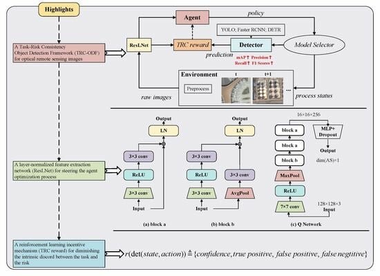
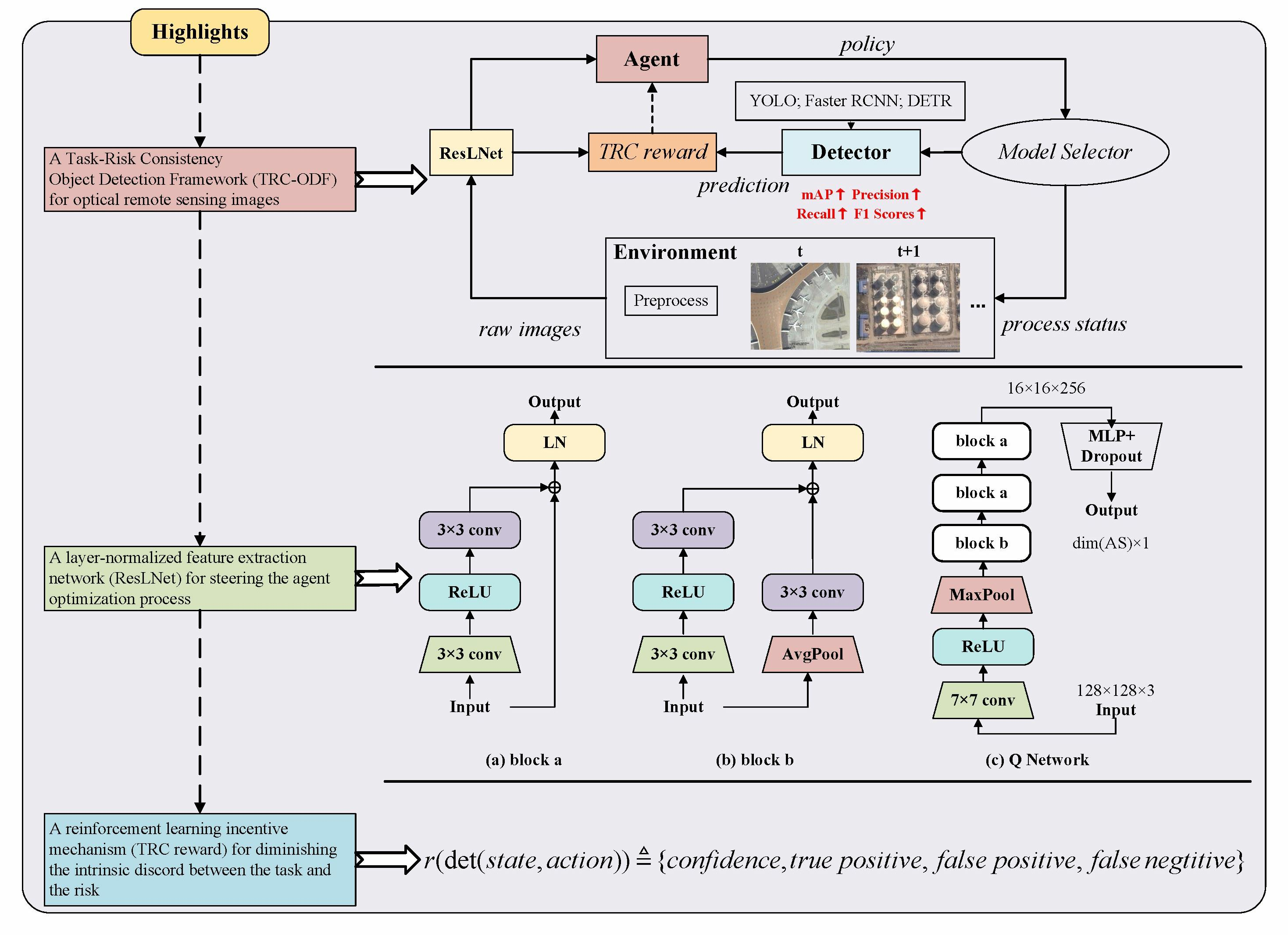
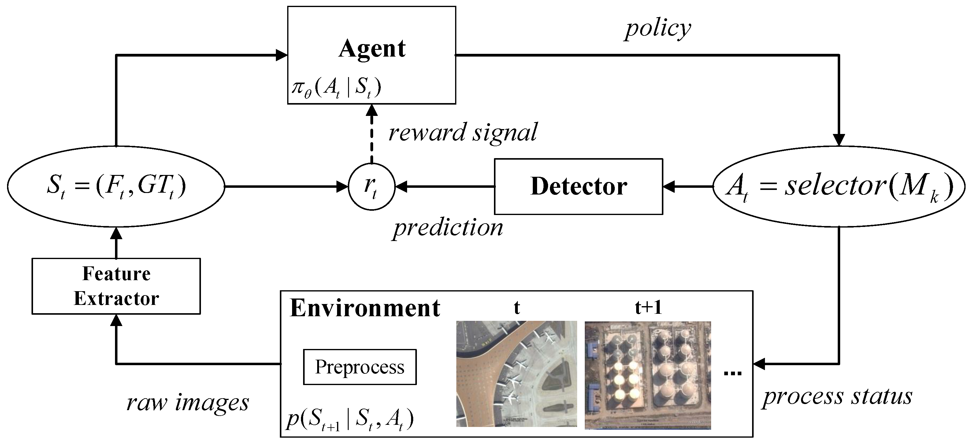
3.1. The Framework of Object Detection Based on Deep Reinforcement Learning

3.1.1. Problem Formulation

This work formulates object detection as a problem in which, for a given input image, $\mathbf{I}\in {\mathbb{R}}^{W\times H\times 3}$ outputs a set of descriptions about object categories and locations:

$${\mathbf{Y}}_{xyc}⫅\left\{{(x_{min},y_{min},x_{max},y_{max},class,conf)}_i\right\},i=1,2,\cdots ,N.$$

(1)

The model obtained through data-driven training can be understood as such a mapping:

$${\mathbf{Y}}_{xyc}=h_k\left({\mathbf{I}}_t\right)$$

(2)

$$h_k\triangleq M_k,k=1,2,\cdots ,P,$$

(3)

where ${\mathbf{I}}_t$ is the tth frame image within an image sequence, while $h_k$ is defined by the network model $M_k$, stored within the model library and comprising weight parameters. Notably, these models can emerge from training on distinct sample sets or as outcomes of diverse network structures and sizes. In practical applications, this study encounters a challenge whereby employing a model trained on a specific sample set fails to meet the detection expectations for certain test samples, despite exhibiting satisfactory performance when evaluated using detection metrics, as depicted in Figure 1. To address this issue, a reinforcement learning model that learns effective optimal policies is proposed, promoting enhanced visual outcomes while adhering rigorously to the principle of task-risk consistency. This reinforcement learning agent model, denoted as ${\pi }_{\theta }\left(A_t\right|S_t)$, selects the appropriate action $A_t$ based on the current state $S_t$, at time t. The state $S_t$, obtained from the tth frame of the image sequence, precisely corresponds to the feature representation of the image frame. The action $A_t$ pertains to the selection of different models $M_k$ from the model library. The chosen model is utilized for object detection, yielding a prediction outcome. These predictions undergo evaluation via the incentive mechanism in Section 3.3, where they are quantified as reward values, serving as feedback to the agent. This facilitates the learning, adjustment, and optimization of the network parameters.

The depicted process is illustrated in Figure 3, where $F_t$ is the feature map obtained from the image frame after undergoing feature extraction, $G{T}_t$ is the true value of the detection outcome, and $r_t$ is the current reward value at the subsequent time step. The probability $p\left(S_{t+1}\right|S_t,A_t)$ encapsulates the transition probability between states. Within the proposed model, this probability assumes a Bernoulli distribution, contingent upon the completion of action selection. While previous studies, as outlined in Section 1, primarily focus on adjusting the bounding boxes for visual enhancement, this work uniquely focuses on learning to optimize the detection results, irrespective of the initialization approach. This distinction enables the applicability of the proposed approach to diverse detection results.

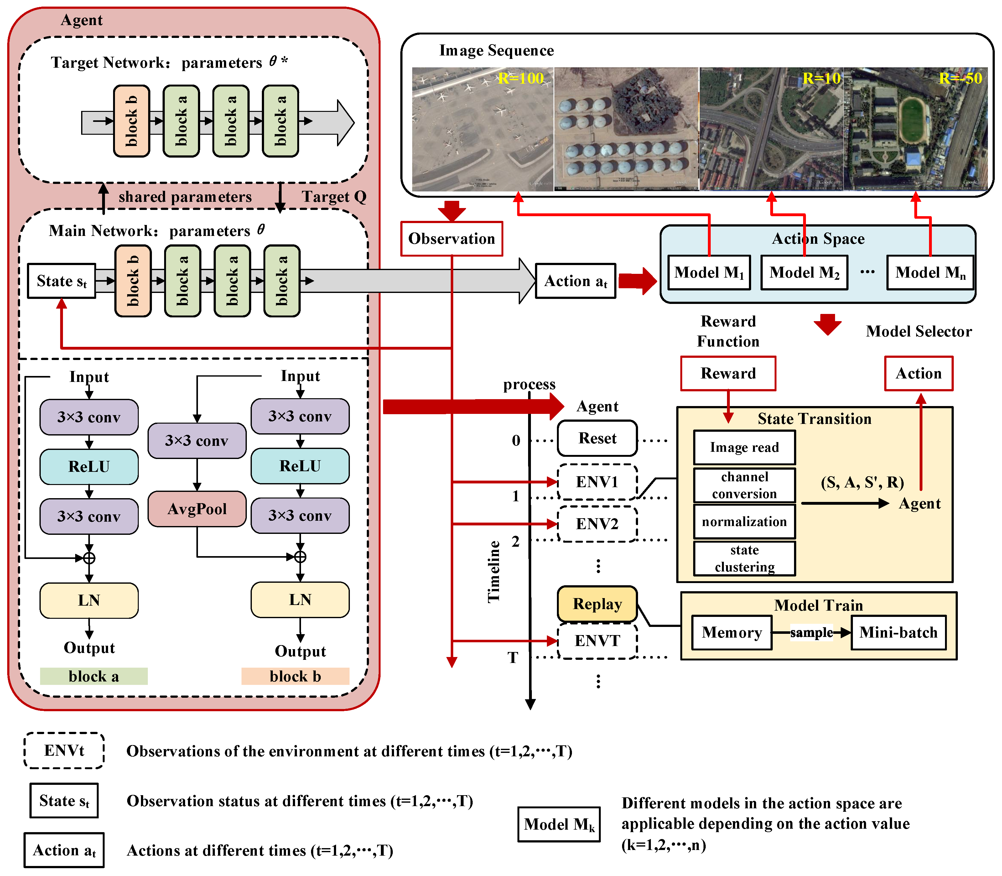
3.1.2. Framework Details

Building upon the aforementioned problem statement, a comprehensive delineation of the framework’s organizational scheme is presented. Next, the framework will be elaborated in detail according to the three parts mentioned above.

The deep reinforcement learning agent serves as a crucial unit responsible for generating strategies that optimize both the models and the results. It engages in policy optimization based on the input state representation, as demonstrated in Figure 2 using the deep Q-network as an illustrative example. This process unfolds through a time-threaded processing flow. Initially, the input optical remote sensing image sequence undergoes preprocessing via environmental observation. Given the typically large size of these images, the preprocessor compresses them to a size of 128 × 128 to facilitate subsequent agent processing. Additionally, the images are normalized based on the pixel mean and variance of the input data. Consequently, the processed optical remote sensing images are obtained as the required input state for the agent. Within the deep reinforcement learning agent, a feature extraction unit extracts features from the preprocessed image, with the proposed blocks serving as an example in Figure 2. The design of these feature extraction network structures can be tailored to the specific requirements of different tasks. Nevertheless, the experiments suggest that overly complex feature extraction structures hinder the agent’s parameter updating process during learning. Subsequently, the output of the feature extraction network flows through the prediction head, culminating in the derivation of the model selection strategy. The spatial dimension of this component is defined based on the number of available models. This strategy then guides the selection of models based on the input from different image frames.

Based on the aforementioned object detection outcomes, the reward mechanism is triggered to compute reward values for the outcomes, contingent upon the content presented in Section 3.3. The reward value generated by this module exerts an influence on the reinforcement learning agent through cumulative and diminishing calculations, aiming to guide the optimization of the strategy function. Reward values are obtained and categorized into current and historical aspects, all of which are archived in the experience playback sequence. During the agent’s learning process, in accordance with the temporal processing flow, certain sampled sequences of states are initially employed for preliminary strategy planning and reward computation, subsequently stored in the experience playback sequence. This segment of information will be re-sampled as a mini-batch, serving as the training data throughout the training process.

Drawing upon the aforementioned exposition of this architectural framework, a comprehensive object detection architecture based on deep reinforcement learning is designed. Its adaptability is evident in its ability to be tailored to distinct requirements, wherein the network structure and optimization technique of the reinforcement learning agent can be customized accordingly. Additionally, different detection models can be selected based on the specific focus of the object detection task. To the best of our knowledge, previous researchers have not pursued similar endeavors. Our approach integrates deep reinforcement learning with computer-vision-based object detection tasks, specifically within the domain of optical remote sensing image processing. Subsequent experimental outcomes substantiate the promising research prospects and practical significance of this work.

3.2. The Model-Free Reinforcement Learning Algorithm Based on Value Function

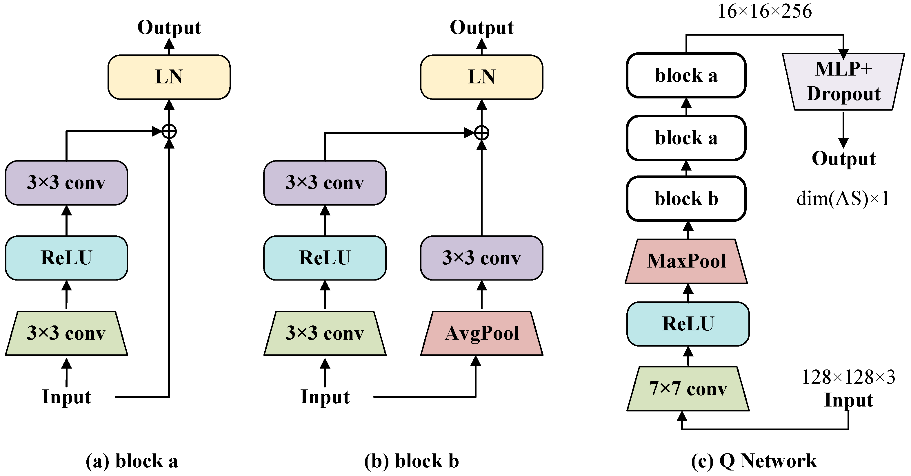
3.2.1. Network Architecture

The most straightforward depiction of a policy involves a lookup table, which constitutes a tabular policy. Reinforcement learning techniques that employ lookup tables are commonly referred to as tabular methods, including Monte Carlo methods, Q-learning, Sarsa, and others. Traditional algorithms in reinforcement learning often employ tables to store the state value function $V\left(s\right)$ or the action value function $Q(s,a)$. However, this approach exhibits significant limitations. In the context of computer vision tasks, reinforcement learning agents encounter continuous image sequences as their state space, giving rise to an infinitely large number of states. Consequently, the table-based approach becomes impractical for storing the value function. To address this challenge, value function approximation employs the function of directly approximating the state-value function or action function. This approach mitigates the storage space requirements and effectively resolves the aforementioned issue.

To compute the value function $Q_{\pi }(s,a)$ within the continuous state and action space formed by models, a function approximation $Q_{\theta }(s,a)$ is employed, referred to as value function approximation:

$$Q_{\theta }(\mathbf{s},\mathbf{a})\approx Q_{\pi }(\mathbf{s},\mathbf{a}),$$

(4)

where $\mathbf{s}$ and $\mathbf{a}$ are the vectorized forms of state s and action a, respectively. The function $Q_{\theta }(\mathbf{s},\mathbf{a})$ typically corresponds to a parameterized function, such as a convolutional neural network, with $\theta$ serving as its parameter. This function yields a real-valued output and is referred to as a Q-network. The deep Q-network employed in this study pertains to the Q-learning technique integrated with deep learning. It primarily combines value function approximation and convolutional neural network technology, utilizing both the object network and experience replay methodology for network training. In traditional Q-learning, a table is utilized to store the rewards acquired by taking specific actions a under each state s, effectively representing the state-value function $Q(s,a)$. However, this approach encounters the challenge of dimensionality in tasks characterized by an extensive state space or even continuous domains, rendering its execution infeasible. Consequently, the utilization of a deep Q-network, which employs the value function approximation technique, proves more suitable for addressing problems associated with the state space.

Diverging from the simplified Atari game screen typically handled by the original deep Q-network, the research necessitates the direct processing of optical remote sensing images by the proposed network. To this end, this work proposes ResLNet, as illustrated in Figure 4, to extract the relevant features from image sequences within the state space.

The network architecture is constructed based on the residual network framework and incorporates layer normalization. It primarily consists of two types of constituent blocks, namely Block A and Block B. Both network blocks share a similar structure. They process the input feature or image through two successive layers of 3 × 3 convolution, followed by a nonlinear activation layer, forming a residual structure that combines the input with the output. Subsequently, the resulting feature map undergoes pixel-wise addition and is eventually passed through a layer normalization layer. However, the two network blocks differ in their respective shortcut paths. In the case of Block B, the initial input requires size compression to match the dimensions of the output feature map for the addition operation. This dimension compression in Block B’s shortcut path is accomplished through an average pooling layer followed by a 3 × 3 convolutional layer. In contrast, Block A maintains consistent dimensions at the junction of the shortcut path and the residual path. The shortcut path in Block A keeps the input unchanged as it traverses through the network.

In contrast to the residual network approach, the proposed ResLNet diverges by eschewing the use of batch normalization layers after each convolutional layer. Instead, layer normalization is utilized following the process of residual summation. Batch normalization is a valuable technique in deep learning, particularly in supervised learning scenarios, where training data are extracted from the dataset in batches, ensuring that each batch conforms to an independently and identically distributed random sample. By establishing a stable training environment, batch normalization calculates stable mean and variance values for normalization, thereby reducing the impact of input covariance shift. However, in the context of reinforcement learning, batch normalization encounters limitations. As reinforcement learning agents must interact with the environment through the experience replay mechanism to acquire training samples, the availability of data cannot be guaranteed from the outset. Consequently, reinforcement learning fails to provide stable training data for batch normalization. Due to the dynamic nature of the training data, batch normalization struggles to adapt to new samples, leading to inaccurate evaluation functions and degraded policy functions. Previous studies [54,55] have also observed that batch normalization exhibits limited efficacy in deep reinforcement learning, often resulting in longer training times and instability, ultimately yielding suboptimal outcomes. In Section 6.1, the experiments empirically investigate the roles of batch normalization and layer normalization, shedding light on their respective impacts.

Furthermore, this work introduces a post-normalization approach by incorporating layer normalization after the residual calculation step. Conversely, a pre-normalization technique involves placing the normalization step before the feature extraction layer. Each approach, post-normalization and pre-normalization, offers distinct advantages. Post-normalization exhibits stronger parameter regularization effects and enhances the robustness of the model. In contrast, pre-normalization mitigates issues related to gradient explosion or vanishing, as certain parameters are directly added at a later stage. Consequently, when the network architecture is not deeply layered, post-normalization may represent a more sensible choice. In Section 6.1, the effects of pre-normalization and post-normalization are empirically studied, exploring their respective impacts and consequences.

3.2.2. Policy Optimization

In the proposed approach, the detection model optimization problem can be understood as a Markov decision process. A Markov decision process can be described via the following elements: state set $S=s_1,s_2,\cdots$; action set $A=a_1,a_2,\cdots$; transition probability function $P(s,a,s^{\prime })$, where $s^{\prime }$ is transformed from s, determined via the completion of action a; and decay factor $\gamma$, where $0\le \gamma \le 1$ and the reward function is $R(s,a)$.

The training of the agent follows the framework of the deep Q-network algorithm. In this work, the agent operates within an environment comprising a sequence of images, with the chosen detection models serving as its actions. The reward assigned to the agent is determined based on the performance of the detection models. The deep Q-network leverages the principles of Q-learning and employs the aforementioned network architecture to estimate the Q-values for each action at every time step, despite the unknown transition probability function. At time step t, the agent updates the Q-value according to the following procedure:

$$Q_{t+1}(\mathbf{s},\mathbf{a})=(\alpha -1)Q_t(\mathbf{s},\mathbf{a})+\alpha (r+\gamma \underset{a^{\prime }}{max}{Q}_t({\mathbf{s}}^{\prime },{\mathbf{a}}^{\prime })).$$

(5)

The agent’s primary objective is to optimize the cumulative reward value during each iteration, as illustrated in Algorithm 1, which outlines the utilization of the iterative deep Q-network algorithm. In the training implementation, this work divides the process into three different stages. In the initial phase, denoted as “experience cache accumulation”, a cache of a certain capacity is established to store state space samples, action selections, and reward changes due to dynamic interactions between the agent and its environment. After completing some time steps dedicated to assembling the experience, the formal training phase begins. An exploration mechanism is introduced during the training process to alleviate the potential dilemma of the agent action selection falling into repeated loops. The final stage of the training scheme involves regular updates of the target network, a key step that facilitates loss calculation and subsequent backpropagation. The update frequency of the target network is set, combined with a safeguard that incrementally integrates 10% of the historical network weights every update. This measure is taken to prevent excessive fluctuations in the network weight update process.

Algorithm 1: Optimization process.

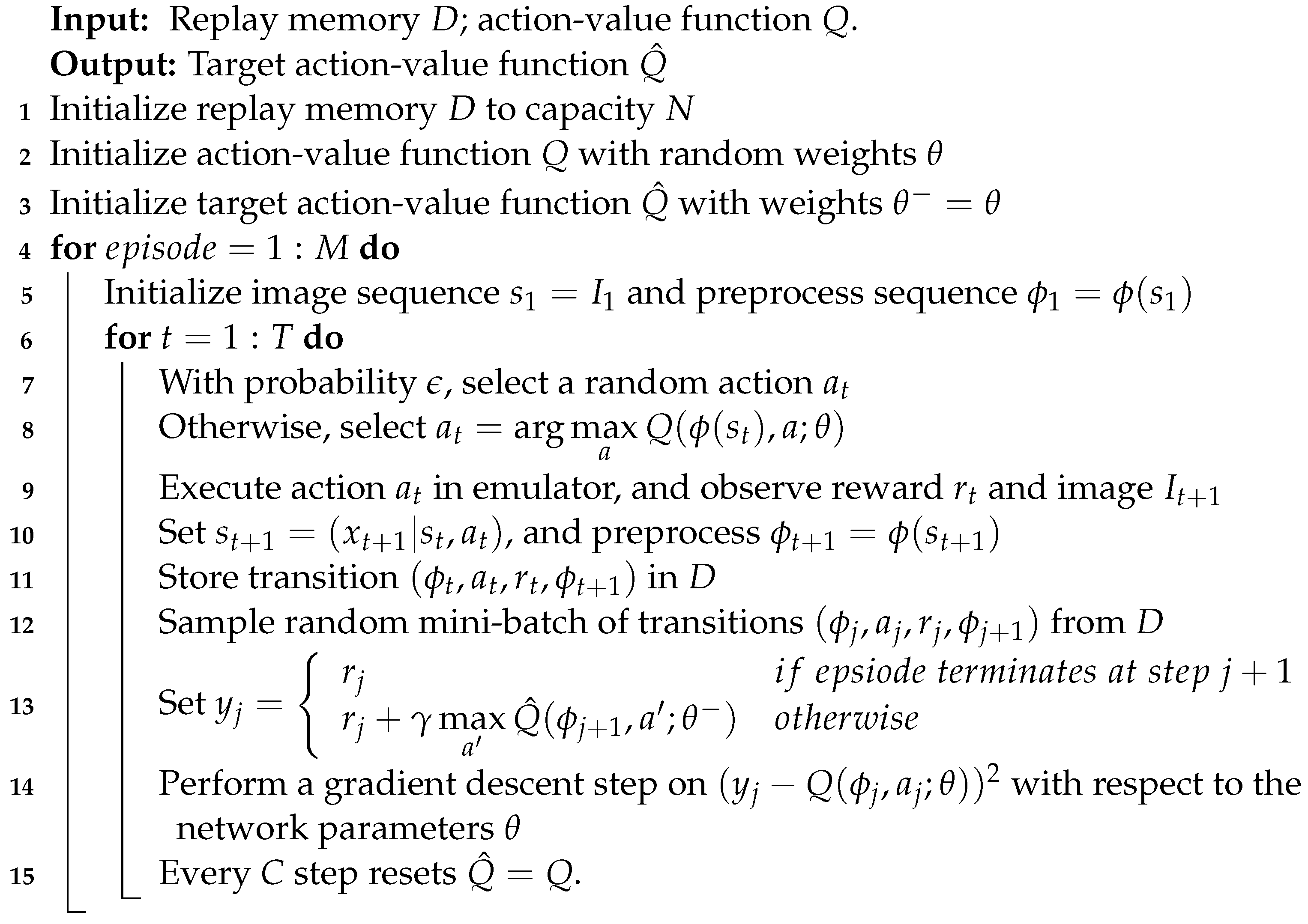
3.3. The Reward Mechanism for Task-Risk Consistency

The mean average precision (mAP), an extensively utilized metric for the evaluation of object detection, has garnered significant attention [56,57,58]. It serves as a valuable tool to assess the performance of object detectors on specific datasets. In applications of reinforcement learning to object detection, it is customary for researchers to employ the mAP as the primary reward mechanism directing the optimization trajectory of the agent. However, this methodology presents inherent constraints. While this metric accounts for factors such as positional deviation and category balance, it should be acknowledged that it does not provide a comprehensive evaluation and overlooks certain aspects. One such aspect is score density, which refers to the specific score distribution associated with each detected object. During the mAP calculation, the focus lies solely on the ordering of all detection results, neglecting the actual scores assigned to the identified objects. Therefore, the impact of the score density on the evaluation of object detection performance should be taken into consideration beyond the conventional mAP metric.

Several key characteristics of the mAP are summarized as follows. (1) An increase in mAP at higher intersection over union (IoU) thresholds does not solely imply improved positional performance. It can also be attributed to instances where the detector fails to filter out certain false positives (FPs) that happen to exhibit superior positional accuracy. Consequently, threshold-based mAP values introduce positive contributions. (2) The impact of FPs on performance is contingent upon the presence of true positives (TPs) with lower scores than the FPs. There are instances where the FPs do not detrimentally affect the performance. To address these challenges, this study proposes a reward mechanism known as task-risk consistency, which guides reinforcement learning agents in their model selection process. During practical predictions, achieving highly accurate detection results remains a primary objective, necessitating a careful assessment of the influence exerted by both FPs and false negatives (FNs) on the overall outcomes. Moreover, the nature of the detection results with varying scores warrants careful consideration. Specifically, for the detection results exhibiting relatively low scores, greater penalties should be assigned to those with higher scores. To this end, a more comprehensive reward mechanism is proposed, which takes into account the confidence associated with the detection results. The specific formulation of the reward function is as follows:

$$r\left(det(s_t,a_t)\right)=[\frac{1}{N_{TP}}\sum _{i=1}^{N_{TP}}con{f}_i^{TP}-\frac{1}{N_{FP}}\sum _{j=1}^{N_{FP}}con{f}_j^{FP}-N_{FN}(1-con{f}_{thres})]\times 100,$$

(6)

where $det(s_t,a_t)$ is the detection result when the input state (image) $s_t$ is the applicable action (model) $a_t$; $N_{TP}$, $N_{FP}$, and $N_{FN}$ are the sample numbers of TP, FP, and FN, respectively; $con{f}_i^{TP}$ and $con{f}_j^{FP}$ are the prediction scores of the corresponding TP and FP samples, respectively; and $con{f}_{thresh}$ is the confidence threshold of the final prediction result output. Further exploration of the proposed reward function is presented through comparative experiments in Section 6.2.

4. Experimental Settings

This section introduces the datasets used in the experiment, the experimental settings, the selected comparison methods, and the evaluation index of the experimental results.

4.1. Parameter Setup

4.1.1. Object Detection Network Training Parameter Settings

All experiments conducted in this study were executed on the Ubuntu operating system, utilizing the PyTorch open-source architecture. The selection of an appropriate learning rate for the network model is a critical factor during the training process. To expedite the convergence of network parameters in the initial training stage, a larger learning rate was set, while a smaller learning rate was subsequently applied to prevent convergence issues during later stages. A warmup period of three epochs was implemented with a learning rate of 0.01. Following the warmup phase, the Adam optimizer was employed with a learning rate of 2.5 × 10${}^{-4}$, dynamically adjusted based on the training status using an adjustment factor of 5 × 10${}^{-4}$. The network operated with a batch size of 32, and the training iterations spanned 200 epochs.

4.1.2. Reinforcement Learning Agent Training Parameter Settings

The agent goes through an extensive training scheme for a total of 500,000 time steps, following three different phases described in Section 3.2.2. A 10,000-capacity cache was established to enable experience replay. The global learning rate was set to 2.5 × 10${}^{-4}$, the batch size was 128, the training frequency was 10 time steps, and the reward discount factor was set to 0.99. The initial exploration rate was initialized to 1 and gradually decayed to a minimum value of 0.05. This exploration mechanism operated exclusively during the first 50% of the training time steps. The update frequency of the target network was set to 100 time steps.

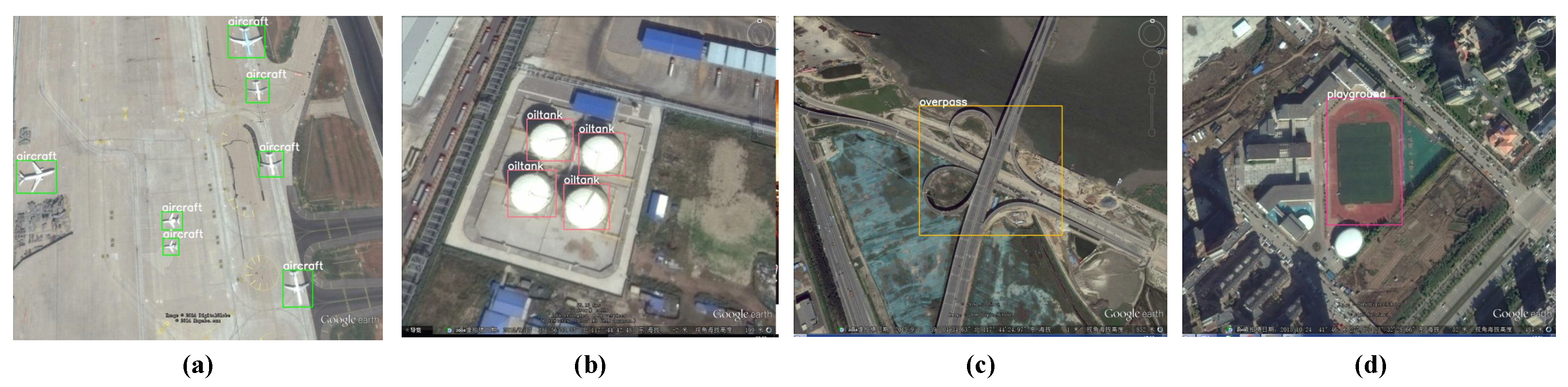
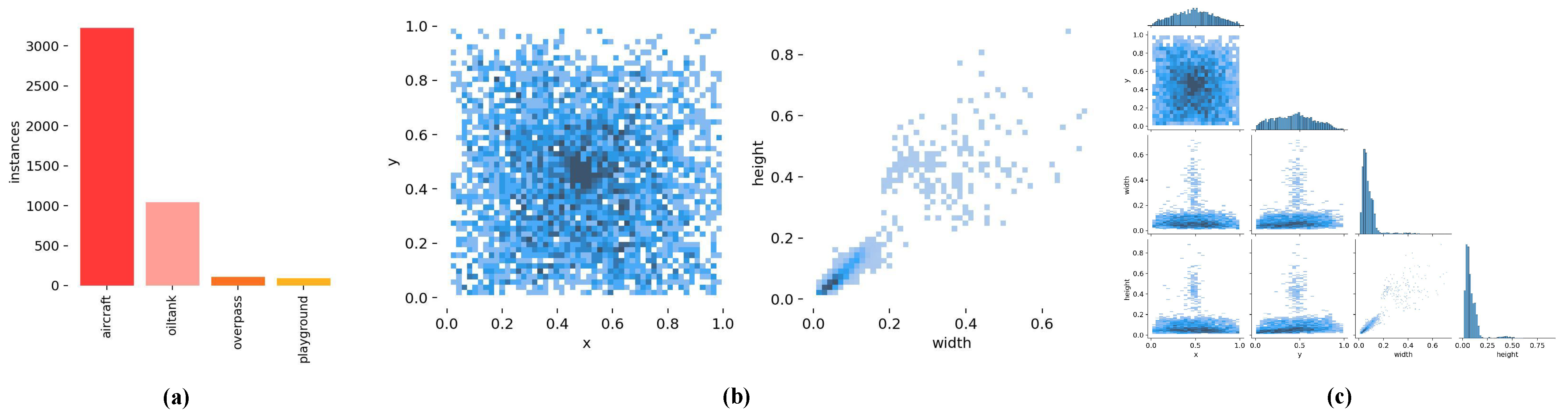
4.2. The Description of the Datasets

Some representative datasets [6,59,60] were selected to conduct the experimental investigations, with comprehensive descriptions given as follows. The RSOD dataset [59] was sourced from Google Earth and Tianditu, encompassing a total of 936 images. These images featured objects categorized into four distinct classes, namely airplane, fuel tank, overpass, and playground, as demonstrated by the annotated ground truth images showcased in Figure 5. Notably, the diverse object categories exhibited varying resolutions, ranging from 0.5 to 2 m for aircraft images, 0.3 to 1 m for fuel tank images, 1.25 to 3 m for overpass images, and 0.4 to 1 m for playground images. The sensors employed in capturing these images comprised panchromatic and multispectral modalities, with image dimensions falling within the size range of $512\times 512$–$1961\times 1193$.

Moreover, a comprehensive analysis was conducted to assess the image count and category distribution within the RSOD dataset, revealing a significant class imbalance, as depicted in Figure 6. Notably, the aircraft category exhibited the largest number of objects and corresponding images, followed by the oil tank. Conversely, the representation of overpasses and sports fields was notably limited, comprising less than 4% of the objects found in the aircraft category. To address the limitations of the original dataset, the study referenced in [59] employed an extensive range of data augmentation techniques, resulting in a remarkable 59-fold increase in the number of objects. Additionally, 2326 background images were introduced as counterexamples. These augmentation methods were carefully designed and tailored to the specific characteristics of each category, ensuring their effectiveness and practical applicability. However, it is important to note that this work does not delve into the intricacies of these complex and specific data augmentation methods, as it is beyond the scope of the research. Instead, the primary objective revolves around optimizing the models and refining the outcomes through the implementation of deep reinforcement learning algorithms within existing model libraries.

In the context of the RSOD dataset, a systematic processing approach was employed to ensure its suitability for analysis. Initially, the positive images for each category were divided into training and testing sets, adhering to a 3:2 ratio. Consequently, a total of 560 images were allocated to the training set, while the remaining 376 images constituted the testing set. Subsequently, the training data underwent an HSV enhancement method, wherein the color gamut parameters for the H, S, and V channels were set to 0.015, 0.7, and 0.4, respectively. Additionally, affine transformations were applied with translation and scaling ratios of 0.1 and 0.5, respectively. Furthermore, a 50% probability was assigned to perform upside-down and left-right flips. To further augment the dataset, a mosaic enhancement technique was employed on all images, involving the fusion of multiple images into a single detection sample. Importantly, these augmentation methods were consistently applied across all datasets, without differentiation based on individual categories.

In order to verify the generalization of the proposed method, the experiments also introduced datasets [6,60] with more complex scenes and more diverse categories as evaluation objects. The NWPU VHR-10 dataset [60] has 10 categories of objects and contains a total of 715 high-spatial-resolution color images from Google Earth and 85 very-high-spatial-resolution pan-sharpened color infrared (CIR) images from Vaihingen dataset [61]. The spatial resolution in Google Earth images ranges from 0.5 to 2 m, and the spatial resolution of the CIR images is 0.08 m. These 800 images contain 150 background images, which were also used in the training process. The remaining images were divided into training sets and testing sets according to 8:2. The DIOR dataset [6] has 20 categories of objects and contains a total of 23,463 optical remote sensing images and 192,472 object instances. The image size in the dataset is 800 × 800 pixels, and the spatial resolution ranges from 0.5 to 30 m. Similar to most existing datasets, this dataset was collected from Google Earth by experts in the field of Earth observation interpretation. In order to ensure the distribution similarity between training data and testing data, the original work randomly selected 11,725 images as the training set and the remaining 11,738 images as the testing set. In order to control the variables as much as possible, the NWPU VHR-10 and DIOR datasets were enhanced in the same way as the RSOD dataset.

4.3. Evaluation Metrics

To quantitatively assess the efficacy of the optimized detection algorithm, several evaluation metrics were employed, namely precision (P), recall (R), mean average precision (mAP) [62], and return. These metrics served as quantitative measures for the evaluation of algorithm performance. In this experiment, P was mainly used to measure the action selection accuracy of the agent, and, at the same time, together with R, it provided the basis for the mAP.

While acknowledging the inherent limitations of the mAP as an incentive for reinforcement learning, this study recognizes its importance as an important reference for algorithm performance evaluation. To determine the average precision (AP) value for an individual category, the enclosed area between the precision–recall (P-R) curve and the coordinate axis was computed. Then, the AP values of all categories were averaged according to the number of categories to obtain the mAP. Finally, different mAP values were calculated, according to different IoU thresholds, and then averaged to obtain the final result. Through the previous comparison, it was found that the reward value can not only reflect the performance of the agent but also reflect the detection performance under the proposed framework. Therefore, the return value was also used as one of the evaluation metrics.

Moreover, the experimental analysis focused on two crucial aspects of the reinforcement learning agent’s performance: the convergence speed and sample efficiency. Notably, the convergence rate cannot be accurately captured by a single formula due to its dependence on the specific learning algorithm and task configuration. However, the convergence rate can be estimated by monitoring performance metrics such as the cumulative reward throughout the training process.

Furthermore, sample efficiency, denoted as $SE$, is expressed as $SE=(R-R_b)/N$, where $SE$ is the sample efficiency, R is the cumulative reward obtained using N samples, and $R_b$ is the baseline reward, typically derived from a randomized policy.

5. Results

In this section, the effectiveness of the TRC-ODF is verified by describing the comparative experiments. These experiments were performed on the RSOD dataset.

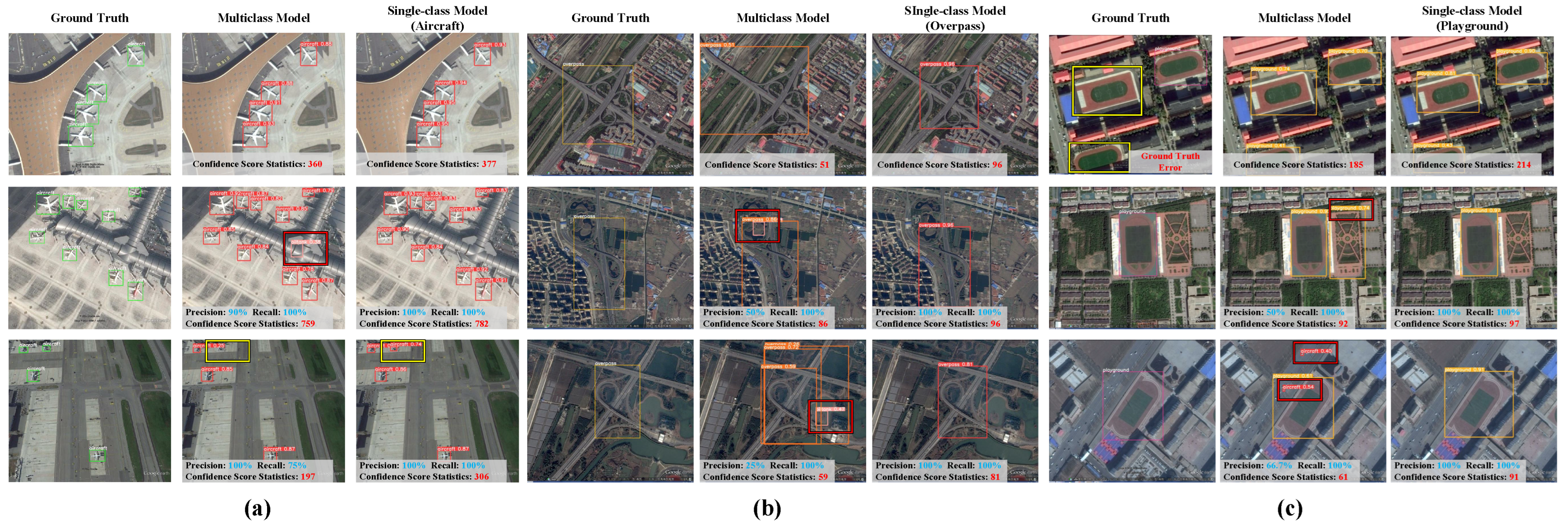
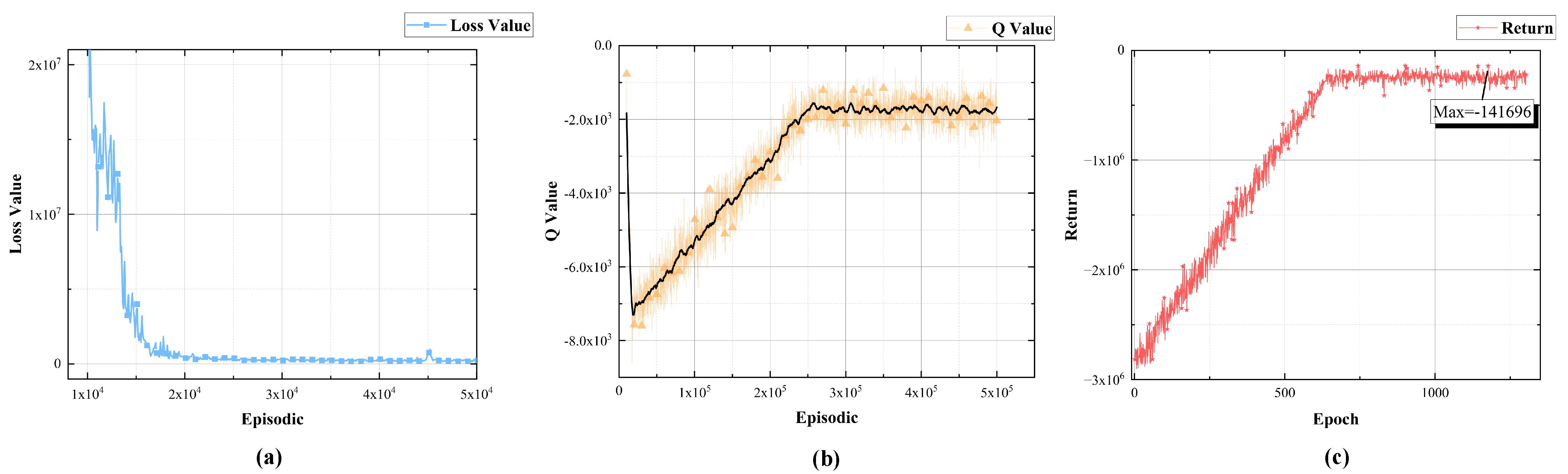
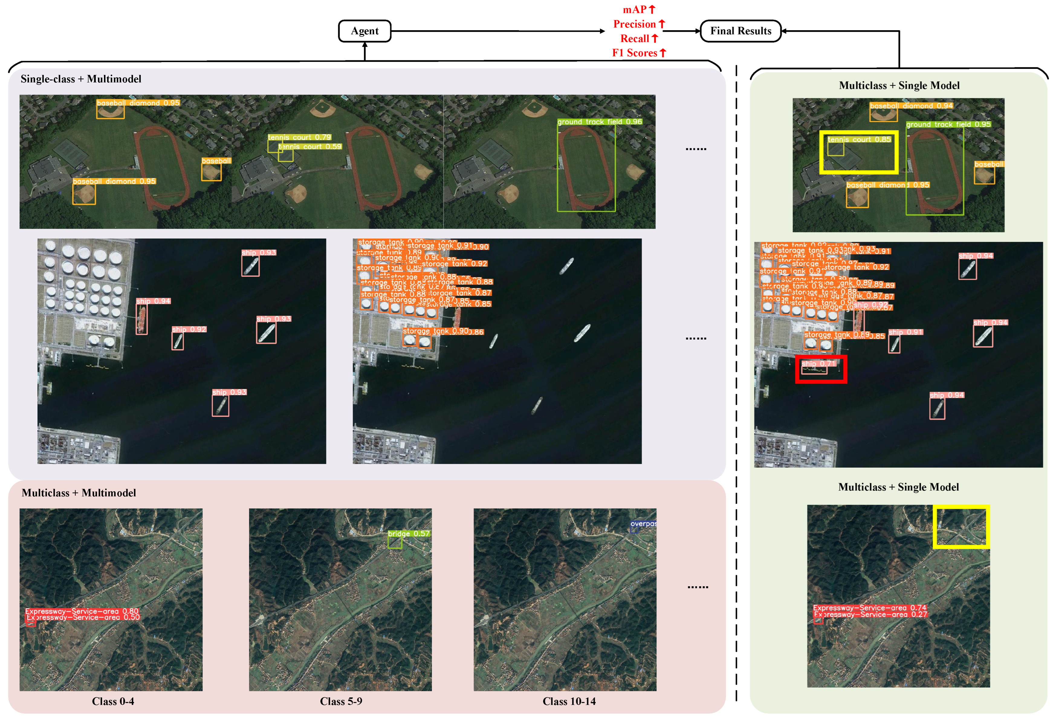
5.1. Experimental Result and Analysis of the Rationality of the Proposed Framework

To verify the robustness and applicability of the proposed framework, five different models were used for evaluation: a multiclass model, designated as M0, and four class-specific models, namely M1, M2, M3, and M4. It is worth noting that M0 was trained on the RSOD dataset, which contains four different categories. In contrast, M1 to M4 focused on the single categories of these objects and were trained on the same RSOD dataset, with other categories and backgrounds described as counterexamples. Following this, a reinforcement learning agent was trained to utilize the outcomes from each model on the RSOD validation set. The agent’s training was then directed by the TRC reward function, enabling it to extract optimization suggestions. Post-training, the agent’s efficiency was assessed on the RSOD validation set, wherein it discerned the most suitable model based on the provided verification set image. A comprehensive analysis of the experimental outcomes revealed several insights. Initially, we observed fluctuations in the agent’s reward curve, Q-value curve, and loss function throughout its training. Subsequently, the total rewards obtained by the agent after training were counted. Conclusively, the efficacy and reasonableness of the proposed approach were ascertained by juxtaposing the model selection outcomes with standard object detection evaluation metrics.

Figure 7 delineates the progression of the reward curve, Q-value curve, and the loss function alterations during the reinforcement learning agent’s training epoch. With iterations as the abscissa across all curves, their respective ordinates represent the return, Q-value, and loss function values. Several critical observations emerged from the depicted curves. Employing the study’s proposed framework and feedback reward mechanism, the agent manifested stable training, culminating in a consistent plateau value. There was marked convergence in the Q-value function, complemented by an ascendant trend in the reward values. A comparative analysis was undertaken between the perceived reward values of the combined category model and its single-category counterpart. Notably, agents leveraging single-model perception amassed higher reward values. This underscored the potency of augmenting the perception and amplifying the detection performance via reinforcement learning. In order to verify the universality of these results, the [email protected] and [email protected]:0.95 were used as evaluation metrics for the final detection results, as shown in

Table 1. Comparison of the reward values and detection performance of multiclass models and the proposed framework.

Dataset	Model		Return		[email protected]		[email protected]:0.95		Precision		Recall		F1 Score
RSOD	Multi- Class	A 1	−91,562.8	−2339.5	90.8	90.6	64.7	64.2	94.3	97.8	92.3	87.3	93.3
		B		3862.7		97.6		78.3		96.1		97.7
		C		−98,131.5		74.9		34.0		84.7		84.9
		D		5045.4		99.9		82.4		98.5		99.3
	TRC-ODF (ours)	A	9058.2	−5699.5	96.2	87.9	67.4	62.1	95.4	96.2	93.9	89.9	94.6
		B		4160.5		97.6		79.3		97.0		98.0
		C		4797.0		99.5		42.6		88.4		87.7
		D		5045.4		99.9		85.7		100.0		100.0
NWPU VHR-10	Multi- Class	a 2	-	-	94.5	99.5	66.9	72.5	94.8	99.1	87.1	100.0	90.8
		b		-		95.4		67.7		91.9		87.4
		c		-		81.4		45.7		81.9		81.0
		d		-		99.0		79.2		97.6		96.7
		e		-		96.7		72.7		96.7		82.4
		f		-		97.0		74.7		96.6		96.2
		g		-		99.9		85.7		100.0		98.2
		h		-		97.3		66.6		95.4		86.9
		i		-		83.8		37.2		94.5		57.6
		j		-		95.4		62.5		94.4		84.9
	TRC-ODF (ours)	a	-	-	96.2	99.5	68.9	75.3	95.2	99.3	93.4	100.0	94.3
		b		-		93.8		68.3		91.1		89.2
		c		-		93.7		43.3		94.5		92.7
		d		-		98.9		81.6		98.2		98.4
		e		-		97.0		71.9		92.8		94.4
		f		-		99.3		81.3		92.9		100.0
		g		-		99.5		92.6		100.0		99.6
		h		-		97.9		68.6		98.3		94.9
		i		-		86.2		38.6		91.9		75.9
		j		-		95.9		67.2		93.5		89.3
DIOR	Multi- Class	1–5 3	-	-	81.8	88.3	61.0	69.1	86.1	91.8	74.1	78.9	79.7
		6–10		-		79.7		62.2		84.8		73.0
		11–15		-		79.5		59.6		82.7		73.0
		15–20		-		79.5		53.0		85.1		71.6
	TRC-ODF (ours)	1–5	-	-	82.6	89.0	61.7	69.5	87.8	91.9	74.7	79.7	80.7
		6–10		-		79.9		62.6		85.6		74.3
		11–15		-		80.4		59.8		85.2		73.1
		16–20		-		80.9		54.7		88.4		71.6

The parts marked in red and bold represent the results of this study. ¹ Classes A, B, C, and D correspond to the aircraft, oil tank, overpass, and playground categories in the RSOD dataset, respectively. ² Classes a–j correspond to the airplane, ship, storage tank, baseball diamond, tennis court, basketball court, ground track field, harbor, bridge, and vehicle categories in the NWPU VHR-10 dataset, respectively. ³ Classes 1–20 correspond to the expressway service area, expressway toll station, airplane, airport, baseball field, basketball court, bridge, chimney, dam, golf field, ground track field, harbor, overpass, ship, stadium, storage tank, tennis court, train station, vehicle, and windmill categories in the DIOR dataset, respectively.

. The superior reward value acquisition and mAP results of the single-class model, post-sensing-agent evaluation, overshadow those of the multiclass model. Specifically, there was an increase of 5.95% in the [email protected] metric, an enhancement of 4.17% in the [email protected]:0.95 metric, and an almost 100,000 increment in the reward value. These metrics robustly vindicate the efficacy of the proposed framework. Furthermore, the proposed framework adeptly addressed data category imbalances. Given the paucity of images and limited objects per image, the multiclass model training inadvertently overlooked Class C objects, culminating in suboptimal prediction outcomes. The framework introduced herein employed a single-class model, offering bespoke mapping for Class C, thereby markedly refining its predictive precision. This exemplifies the framework’s resilience across varied data scenarios.

In addition, in order to further verify the robustness and generalization of the proposed framework, this work also conducted the same experiments on the NWPU VHR-10 dataset and the DIOR dataset. Since the NWPU VHR-10 dataset contained a total of 10 categories, the experiment on this dataset used one multi-class hybrid model and 10 single-class models. They were all trained on the same dataset, and other categories and backgrounds were described as negative. Since the DIOR dataset contained more object categories (20 categories), this experiment used a slightly different processing method for this dataset. These 20 categories were divided into four groups, each group containing five categories of objects; thus, a total of five multiclass mixture models were used. One model contained all categories, and the remaining four models contained five categories each. The rest of the settings were the same as for the experiments on the RSOD dataset. The results involving these two datasets are combined in Table 1.

Figure 8 presents partial visualization prediction results on the NWPU VHR-10 and DIOR datasets. The left half, separated by dashed lines in the figure, represents alternative predictions composed of multiple models, while the right half represents the detection results obtained from the original detection network. In the proposed framework, trained agents optimize the predictions generated by the multiple models. Compared with a single model, the proposed framework performed better in the final results. By making full use of the prediction results of multiple models, objects that cannot be detected by a single model can be predicted, and false detections caused by multiclass models can also be avoided.

5.2. Experimental Results and Analysis of Different Scale Detectors

To substantiate the rigor and extensibility of the proposed TRC-ODF framework, additional experiments were conducted using YOLOv8 detectors of disparate scales. Unlike the preceding assessments, the models employed here featured distinct network architectures, although they were uniformly trained on the comprehensive RSOD dataset, thereby complementing the prior experiments. Five YOLOv8 detectors of varying dimensions were selected and subjected to mAP evaluation post-training, as enumerated in

Table 2. Performance comparison between isolated models of different scales and multimodels based on deep reinforcement learning.

Model		Selected Percentage	[email protected]	[email protected]:0.95	Precision	Recall	F1 Score
Single Model	YOLOv8-n	-	87.1	53.7	90.5	87.7	89.1
	YOLOv8-s	-	90.8	64.7	94.3	92.3	93.3
	YOLOv8-m	-	94.5	72.4	96.0	93.2	94.6
	YOLOv8-l	-	96.8	76.3	96.6	94.8	95.7
	YOLOv8-x	-	98.7	77.7	98.1	95.7	96.9
Multimodel (RL)	YOLOv8-n	0.0%	98.9	80.1	98.3	96.6	97.4
	YOLOv8-s	0.0%
	YOLOv8-m	1.9%
	YOLOv8-l	2.8%
	YOLOv8-x	95.3%
Single Model	Faster R-CNN	-	94.9	68.0	95.9	91.7	93.8
	DETR	-	95.5	69.4	96.5	93.5	95.0
Multimodel (RL)	Faster R-CNN	90.0%	96.5	68.6	97.4	92.9	95.1
	DETR	90.1%	97.4	69.8	97.9	95.9	96.9

The parts marked in red and bold represent the results of this study.

. The findings unambiguously indicate that the larger detectors generally outperformed their smaller counterparts in detection tasks. Given that even expansive network configurations cannot guarantee universal optimization across all validation sets, the detailed outcomes are given in Table 2, where the relative prevalence of differently scaled models selected by the sensing agent is accounted for. The objective was to discern efficacious models across varying scales that maximize resource utility within the model library. Detailed results are recorded in Table 2, which takes into account the relative proportions of the models of different sizes chosen by the agent. Notably, while the most intricate model demonstrated superior prediction capabilities in most scenarios, the second-largest or the third-largest model exhibited comparable performance in specific instances. In quantitative terms, the [email protected] index was marginally elevated by 0.2, while the [email protected]:0.95 index experienced a more substantial increase of 2.4. This substantiates that even scaled down models can make salient contributions to the final evaluation metrics, thereby bolstering the overarching framework’s efficacy in detection tasks.

In addition, this work also conducted experiments on detectors with different network structures from the YOLO series, namely Faster R-CNN and DETR. Faster R-CNN is one of the classical object detection algorithms, while DETR adopts the Transformer structure that is currently highly respected, which is a different network from YOLOv8. Using the same method for framework adaptation, it can be observed from Table 2 that the proposed framework can also improve the detection performance.

6. Discussion

The ensuing section is dedicated to describing the ablation experiments to elucidate the underpinnings of the TRC-ODF framework. The investigative focus predominantly encompasses the architectural nuances of the feature extractor’s network and the formulation of the reward function. Concomitantly, this work furnishes a rigorous analysis of the computational expenses, encompassing both temporal and storage overheads, attributable to the deployment of the proposed framework.

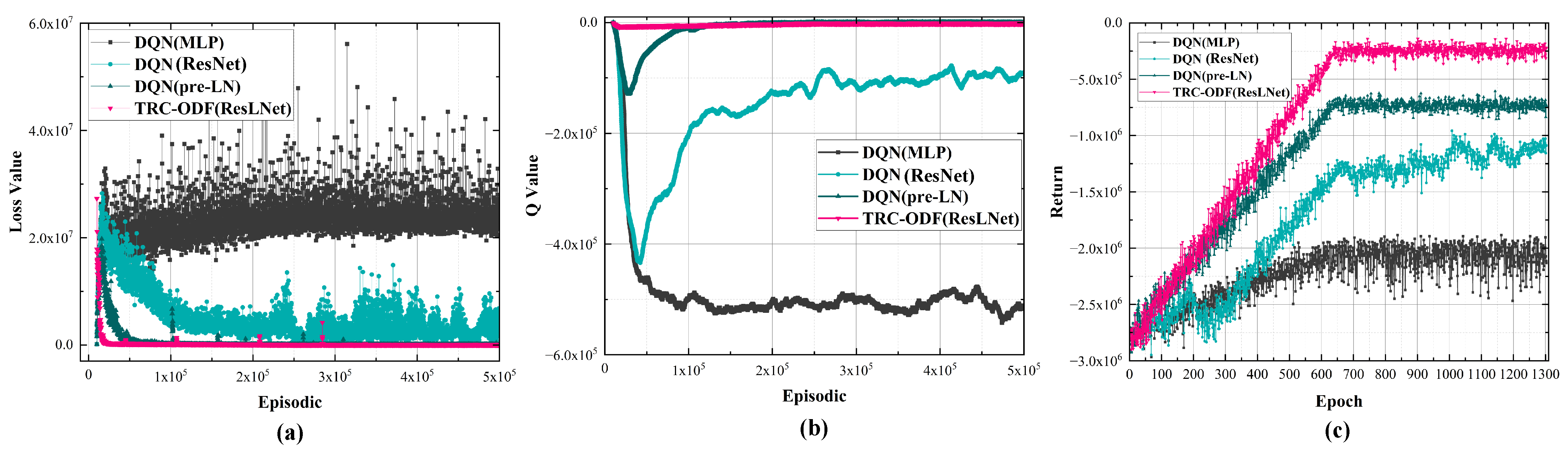
6.1. Effectiveness of the Agent Feature Extractor

The proposed ResLNet, with a distinct architectural design for the feature extractor, diverges from the conventional structures prevalent in extant reinforcement learning models. Our approach uses the post-layer normalization technique, advancing the traditional residual network. For an intricate visual representation, the reader is directed to Figure 4. To validate its efficiency, it was juxtaposed against a suite of feature extractors: the prototypical one, the ResNet feature extractor with an embedded residual structure, and the strategy integrating prelayer normalization within the DQN framework. Drawing upon comparative metrics, the terminal reward value, and the detection evaluation indices [email protected] and [email protected]:0.95, the superiority of the post-layer normalization method delineated in this work is emphatically evidenced.

The aforementioned figure provides a detailed view of the training trajectories for distinct network architectures. Specifically, Figure 9a,b unequivocally demonstrate the merits of post-layer normalization, with outcomes indicating enhanced convergence rates, superior sample efficiency, and a consistent Q value. Subsequently, Figure 9c affirms the potential of this technique to yield elevated reward values. Such observations lend credence to the prior discourses surrounding layer and batch normalization. Within the realm of deep reinforcement learning, layer normalization fosters augmented stability and mitigates adverse exploration tendencies. Through this empirical experiment, the superiority of post-layer normalization over prelayer normalization was also identified, which aligns with the analytical assertions in Section 3.2.1. These empirical nuances are manifested in the acquired reward metrics and conclusive detection performance evaluations, as

Table 3. Comparison of the impact of different feature extractors on reward value and detection performance under the same perceptual intelligence framework.

Network		Return		[email protected]		[email protected]:0.95		Precision		Recall		F1 Score
DQN (MLP)	Class A	−6046.4	−6046.4	22.0	87.9	15.5	62.1	24.1	96.2	22.5	89.9	23.2
	Class B		0.0		0.0		0.0		0.0		0.0
	Class C		0.0		0.0		0.0		0.0		0.0
	Class D		0.0		0.0		0.0		0.0		0.0
DQN (ResNet)	Class A	942.6	−6475.7	59.7	81.0	45.7	57.7	98.1	97.9	59.9	81.7	74.4
	Class B		4242.0		97.6		79.3		94.4		98.8
	Class C		925.3		20.8		10.8		100.0		20.0
	Class D		2251.1		39.6		35.1		100.0		39.1
DQN (pre-LN)	Class A	3616.4	−6046.4	69.1	87.9	54.4	62.1	96.1	96.2	70.4	89.9	81.3
	Class B		4153.0		95.6		77.4		94.5		96.3
	Class C		86.9		2.0		1.6		100.0		1.7
	Class D		5422.9		91.0		76.4		93.8		93.8
TRC-ODF (ResLNet)		9058.2		96.2		67.4		95.4		93.9		94.6

The parts marked in red and bold represent the results of this study.

shows. When juxtaposed against network paradigms such as MLP, CNN(ResNet), and pre-LN, the TRC-ODF (ResLNet) methodology proposed herein improves the [email protected] index by 337.3%, 61.1%, and 39.2% respectively. Analogously, the [email protected]:0.95 metric showed enhancements of 334.8%, 47.5%, and 23.9%.

6.2. Effectiveness of the Reward Function Based on Task-Risk Consistency

Within the domain of deep reinforcement learning, the reward function stands as an elemental cornerstone, decisively charting the agent’s optimization trajectory. Drawing from the paradigm of task-risk consistency, this study introduces a reward mechanism using Equation (6) that eschews the direct application of the confidence or mAP as incentive measures. To verify the effectiveness of the designed mechanism, this work compared it with two alternative object detection rewards, as shown in

Table 4. Comparison of the impact of different reward mechanisms on the reward value and detection performance under the same perceptual intelligence framework.

Reward Model		Select Accuracy		[email protected]		[email protected]:0.95		Precision		Recall		F1 Score
Simple conf.	Class A	95.3%	99.4%	87.1	87.0	60.4	62.0	97.8	95.3	88.3	87.9	91.7
	Class B		100.0%		97.6		79.3		94.1		98.8
	Class C		93.1%		89.3		37.6		93.1		90.0
	Class D		80.0%		74.5		62.5		96.1		76.6
mAP	Class A	96.1%	100.0%	88.2	87.9	61.3	62.1	96.2	97.8	89.1	88.1	92.5
	Class B		100.0%		97.6		79.3		94.1		98.8
	Class C		91.4%		87.9		37.1		96.4		88.3
	Class D		85.0%		79.5		66.6		96.3		81.3
TRC (ours)	Class A	99.7%	100.0%	96.2(+9.1, +8.0)		67.4(+7.0, +6.1)		95.4		93.9(+5.6, +4.8)		94.6(+2.1, +2.9)
	Class B		100.0%
	Class C		98.3%
	Class D		100.0%

The parts marked in red and bold represent the improvement of our method to other reward mechanisms.

. The first approach employed rudimentary confidence levels as immediate reward stimuli; while confidence is not a definitive detection metric, it offers constructive directionality to the agent. Conversely, the second technique leveraged the mAP evaluation index as its incentive mechanism. Notwithstanding its intuitive appeal as a seemingly potent mechanism, the preceding analyses show that such guidance may not invariably culminate in accurate prediction outcomes.

As depicted in Figure 10, normalized training curves were initially obtained corresponding to diverse reward mechanisms to facilitate straightforward comparative analysis. While Figure 10b,c reveal broad congruence in the Q-value and reward normalization curves across the three mechanisms under consideration, Figure 10a indicates that TRC (our method) achieves notably expedited convergence rates and elevated sample efficiency. Further corroboration of the superiority of TRC emerges from the subsequent tabular enumeration of the numerical results. Although the overall trends of the normalized curves bear a resemblance, a closer examination of the actual metrics reveals the advantageous nature of the TRC, particularly in optimizing weaker categories such as Class C and Class D. This is reflected in the heightened selection accuracy in the post-perceptual evaluation in Table 4. Our method also manifests a distinct edge in mAP-related metrics, a testament to the synergistic alignment between the scrupulously crafted task-risk consistency reward mechanism and the overarching framework. This result can be attributed to the proposed, more comprehensive reward mechanism that considers both the detection accuracy and confidence, thus placing more emphasis on the consistency of the model performance with the prediction results, rather than merely considering the mAP metric.

Furthermore, this experiment conducted a more detailed visual analysis of the drawbacks of directly using mAP as a reward and discussed the reasons for this phenomenon. Figure 11 illustrates that the two detectors exhibited identical mAP values but displayed substantial variations in their respective score distributions. In the left image, for instance, the two false positive (FP) scores are 0.87 and 0.88, whereas, in the right image, they are 0.35 and 0.25. These discrepancies in FP scores imply differences in the specific scores assigned by the detectors. Consequently, during practical prediction scenarios, the detector on the right can effectively adjust the score threshold within the range of 0.35 to 0.88, capitalizing on the significant score gap between true positives (TP) and FP. Conversely, the detector on the left can only set the score threshold between 0.87 and 0.88, posing challenges in suppressing the TP results of other images. Furthermore, a lower score threshold is often set during actual prediction, leading to the retention of these two FP results.

In addition, intriguing findings arose in this experiment. Figure 12 presents empirical evidence that may appear counterintuitive. Intuitively, one might expect the detection outcomes of objects labeled as (b) and (d) to be superior to those of (a) and (c) due to the additional false positives (FP) present in (b) and (d). Furthermore, the result for (c) surpassed that of (a) due to its enhanced positional accuracy. Intuitively ranking these results by their mAP might suggest the following order: (c) > (a) > (b) = (d). However, the actual mAP values associated with these four result groups are presented in Figure 12: (c) = (d) > (b) > (a). mAP is calculated by computing the mean average precision for each intersection over union (IOU) threshold and subsequently averaging these values to yield the final result. Although the detection outcomes for (b) contain an FP, when calculating the [email protected], a result with a lower score that has improved positional accuracy does not impact the mAP (since there are no true positives with lower scores, the false positives have no effect on the precision–recall curve). Similarly, when calculating the [email protected], a result with a higher score but poorer positional accuracy becomes an FP. However, as there are no true positives at this threshold in (a), the mAP of (b) remains higher than that of (a). Consequently, for all thresholds considered, the mAP for (b) is either superior to or equal to that of (a), leading to the counterintuitive observation.

The distinction between (c) and (b) lies in the absence of any detection results with inferior positional accuracy in (c). Consequently, when computing a low-threshold mAP such as [email protected], the two are identical (the reason for the lack of negative impact from false positives in (b) remains consistent, as explained above). However, when calculating a high-threshold mAP such as [email protected], (c) outperforms (b), resulting in superior overall performance for (c). Although the intuitive effect of (b) and (d) may appear similar, the discrepancy in the mAP arises from the sole dissimilarity between (b) and (d): the detection result with improved positional accuracy in (d) possesses a higher score. Thus, the performance of (d) aligns with that of (c) since the low-scoring false positives, which exhibit subpar performance, do not influence the outcome.

During the mAP calculation, the detector employs a lower confidence threshold (typically set to 0.001 by default) during the verification phase, enabling the inclusion of a larger number of prediction results in the calculation. However, in practical applications, most predictions with low confidence scores are suppressed. Considering the ultimate objective of the object detection task, incorporating a larger number of prediction results in mAP calculations entails certain risks. Figure 13 illustrates the scenario where the detector in the right image produces a prediction result with a low score but within the IoU threshold. Intuitively, one would expect the performance of the detector on the left to surpass that of the right. However, upon calculating the mAP, it becomes evident that the mAP for the right image is higher. This phenomenon arises because, when calculating the mAP at the low IoU threshold, there are no TPs with scores lower than the FP in question. Conversely, when calculating the mAP at the high IoU threshold, the FP contributes positively to the performance. Consequently, the detector in the right image achieves a higher mAP. This counterintuitive result aligns with the findings presented in the previous section regarding visualizations. To mitigate this, detection results are filtered for retention by establishing score and IoU thresholds. Subsequently, the results are sorted based on confidence. TP and FP are then determined according to the IoU criteria. Finally, the occurrences of FNs are counted, and the reward value is computed as in Equation (6). By employing the proposed reward mechanism for evaluation, the intuitive results align consistently.

6.3. Computational Time Analysis

Given the juxtaposition of the proposed framework with an object detection system, it becomes imperative to discern the temporal and computational overheads introduced during the model’s prediction phase. This work meticulously enumerates key metrics such as the storage requisites of the model, its parameter count, the floating-point operations involved, and any latency engendered by the framework’s incorporation.

Table 5. Computational time analysis.

Model	Size	Parameters	GFLOPs	Delay
TRC-ODF	12.2 MB	3.04 M	1.84	13.2 ms
YOLOv8-s	22.6 MB	11.20 (+8.16) M	28.60 (+26.76)	3.5 (−9.7) ms

elucidates that the post-training model size of the deep reinforcement learning agent was a mere 12.2 MB, signifying minimal storage implications. Concurrently, both the parameter tally and the floating-point operations remained lower than for the standalone model, underscoring the framework’s efficiency. Consequently, the amalgamated system ensured a negligible computational burden during prediction, maintaining a commendable 60 FPS throughput.

7. Conclusions

This study proposes TRC-ODF, a deep-reinforcement-learning-guided task-risk consistency object detection framework tailored for optical remote sensing images. The framework leverages the power of deep reinforcement learning combined with the task-risk consistency reward, with the overall goal of enhancing the detection performance. The core of the proposed framework is a post-layer-normalized feature extraction network based on a residual architecture and a carefully designed reward function, which can extract features from the state space of the agent input and guide the agent to optimize on an accurate trajectory. Complementing the theoretical elaboration of the method, empirical evaluations were performed on various representative optical remote sensing image datasets. These experiments confirmed the logical basis and expected applicability of TRC-ODF and verified the effectiveness of the proposed network and reward mechanism. In view of the overlap in the processing flows of different computer vision tasks, the potential of TRC-ODF under other vision tasks besides object detection can be recognized. The future goal of this research is to generalize the framework to a range of vision tasks, including, but not limited to, classification, tracking, segmentation, and matching. It is expected to connect different computer vision tasks at a higher level through deep reinforcement learning.

References

1. Cheng, G.; Han, J. A survey on object detection in optical remote sensing images. ISPRS J. Photogramm. Remote. Sens. 2016, 117, 11–28. [Google Scholar] [CrossRef]
2. Zhang, F.; Du, B.; Zhang, L.; Xu, M. Weakly Supervised Learning Based on Coupled Convolutional Neural Networks for Aircraft Detection. IEEE Trans. Geosci. Remote. Sens. 2016, 54, 5553–5563. [Google Scholar] [CrossRef]
3. Aposporis, P. Object Detection Methods for Improving UAV Autonomy and Remote Sensing Applications. In Proceedings of the 2020 IEEE/ACM International Conference on Advances in Social Networks Analysis and Mining (ASONAM), The Hague, The Netherlands, 7–10 December 2020; pp. 845–853. [Google Scholar] [CrossRef]
4. Barrett, E.C. Introduction to Environmental Remote Sensing; Routledge: New York, NY, USA, 1999. [Google Scholar]
5. Kamusoko, C. Importance of Remote Sensing and Land Change Modeling for Urbanization Studies. In Urban Development in Asia and Africa: Geospatial Analysis of Metropolises; Murayama, Y., Kamusoko, C., Yamashita, A., Estoque, R.C., Eds.; Springer: Singapore, 2017; pp. 3–10. [Google Scholar] [CrossRef]
6. Li, K.; Wan, G.; Cheng, G.; Meng, L.; Han, J. Object detection in optical remote sensing images: A survey and a new benchmark. ISPRS J. Photogramm. Remote. Sens. 2020, 159, 296–307. [Google Scholar] [CrossRef]
7. Li, C.; Cheng, G.; Wang, G.; Zhou, P.; Han, J. Instance-Aware Distillation for Efficient Object Detection in Remote Sensing Images. IEEE Trans. Geosci. Remote. Sens. 2023, 61, 1–11. [Google Scholar] [CrossRef]
8. Zhang, T.; Zhang, X.; Zhu, P.; Jia, X.; Tang, X.; Jiao, L. Generalized few-shot object detection in remote sensing images. ISPRS J. Photogramm. Remote. Sens. 2023, 195, 353–364. [Google Scholar] [CrossRef]
9. Chen, S.; Zhao, J.; Zhou, Y.; Wang, H.; Yao, R.; Zhang, L.; Xue, Y. Info-FPN: An Informative Feature Pyramid Network for object detection in remote sensing images. Expert Syst. Appl. 2023, 214, 119132. [Google Scholar] [CrossRef]
10. Zhou, H.; Ma, A.; Niu, Y.; Ma, Z. Small-Object Detection for UAV-Based Images Using a Distance Metric Method. Drones 2022, 6, 308. [Google Scholar] [CrossRef]
11. Liu, H.; Yu, Y.; Liu, S.; Wang, W. A Military Object Detection Model of UAV Reconnaissance Image and Feature Visualization. Appl. Sci. 2022, 12, 12236. [Google Scholar] [CrossRef]
12. Kreutzer, J.; Khadivi, S.; Matusov, E.; Riezler, S. Can Neural Machine Translation be Improved with User Feedback? arXiv 2018, arXiv:cs.CL/1804.05958. [Google Scholar]
13. Stiennon, N.; Ouyang, L.; Wu, J.; Ziegler, D.; Lowe, R.; Voss, C.; Radford, A.; Amodei, D.; Christiano, P.F. Learning to summarize with human feedback. Adv. Neural Inf. Process. Syst. 2020, 33, 3008–3021. [Google Scholar]
14. Pinto, A.S.; Kolesnikov, A.; Shi, Y.; Beyer, L.; Zhai, X. Tuning computer vision models with task rewards. arXiv 2023, arXiv:2302.08242. [Google Scholar]
15. Ouyang, L.; Wu, J.; Jiang, X.; Almeida, D.; Wainwright, C.; Mishkin, P.; Zhang, C.; Agarwal, S.; Slama, K.; Ray, A.; et al. Training language models to follow instructions with human feedback. Adv. Neural Inf. Process. Syst. 2022, 35, 27730–27744. [Google Scholar]
16. Liu, P.; Yuan, W.; Fu, J.; Jiang, Z.; Hayashi, H.; Neubig, G. Pre-Train, Prompt, and Predict: A Systematic Survey of Prompting Methods in Natural Language Processing. ACM Comput. Surv. 2023, 55, 1–35. [Google Scholar] [CrossRef]
17. Uzkent, B.; Yeh, C.; Ermon, S. Efficient Object Detection in Large Images Using Deep Reinforcement Learning. In Proceedings of the IEEE/CVF Winter Conference on Applications of Computer Vision, Snowmass Village, CO, USA, 1–5 March 2020; pp. 1824–1833. [Google Scholar]
18. Jie, Z.; Liang, X.; Feng, J.; Jin, X.; Lu, W.; Yan, S. Tree-Structured Reinforcement Learning for Sequential Object Localization. Adv. Neural Inf. Process. Syst. 2016, 29, 29. [Google Scholar]
19. Wang, Y.; Zhang, L.; Wang, L.; Wang, Z. Multitask Learning for Object Localization With Deep Reinforcement Learning. IEEE Trans. Cogn. Dev. Syst. 2019, 11, 573–580. [Google Scholar] [CrossRef]
20. Pirinen, A.; Sminchisescu, C. Deep Reinforcement Learning of Region Proposal Networks for Object Detection. In Proceedings of the 2018 IEEE/CVF Conference on Computer Vision and Pattern Recognition, Salt Lake City, UT, USA, 18–23 June 2018; pp. 6945–6954. [Google Scholar] [CrossRef]
21. Dalal, N.; Triggs, B. Histograms of oriented gradients for human detection. In Proceedings of the 2005 IEEE Computer Society Conference on Computer Vision and Pattern Recognition (CVPR’05), San Diego, CA, USA, 20–25 June 2005; Volume 1, pp. 886–893. [Google Scholar]
22. Lowe, D.G. Distinctive Image Features from Scale-Invariant Keypoints. Int. J. Comput. Vis. 2004, 60, 91–110. [Google Scholar] [CrossRef]
23. Yan, J.; Lei, Z.; Wen, L.; Li, S.Z. The Fastest Deformable Part Model for Object Detection. In Proceedings of the IEEE Conference on Computer Vision and Pattern Recognition, Columbus, OH, USA, 23–28 June 2014; pp. 2497–2504. [Google Scholar]
24. Ren, S.; He, K.; Girshick, R.; Sun, J. Faster R-CNN: Towards Real-Time Object Detection with Region Proposal Networks. Adv. Neural Inf. Process. Syst. 2015, 28. [Google Scholar] [CrossRef]
25. Cai, Z.; Vasconcelos, N. Cascade R-CNN: Delving Into High Quality Object Detection. In Proceedings of the IEEE Conference on Computer Vision and Pattern Recognition, Salt Lake City, UT, USA, 18–23 June 2018; pp. 6154–6162. [Google Scholar]
26. Liu, W.; Anguelov, D.; Erhan, D.; Szegedy, C.; Reed, S.; Fu, C.Y.; Berg, A.C. SSD: Single Shot MultiBox Detector. In Proceedings of the Computer Vision—ECCV 2016: 14th European Conference, Amsterdam, The Netherlands, 11–25 October 2016; Leibe, B., Matas, J., Sebe, N., Welling, M., Eds.; Springer: Berlin/Heidelberg, Germany, 2016; pp. 21–37. [Google Scholar] [CrossRef]
27. Lin, T.Y.; Goyal, P.; Girshick, R.; He, K.; Dollar, P. Focal Loss for Dense Object Detection. In Proceedings of the IEEE International Conference on Computer Vision, Venice, Italy, 22–29 October 2019; pp. 2980–2988. [Google Scholar]
28. Tian, Z.; Shen, C.; Chen, H.; He, T. FCOS: Fully Convolutional One-Stage Object Detection. In Proceedings of the IEEE/CVF International Conference on Computer Vision, Seoul, Republic of Korea, 27 October–2 November 2019; pp. 9627–9636. [Google Scholar]
29. Duan, K.; Bai, S.; Xie, L.; Qi, H.; Huang, Q.; Tian, Q. CenterNet: Keypoint Triplets for Object Detection. In Proceedings of the IEEE/CVF International Conference on Computer Vision, Seoul, Republic of Korea, 27 October–2 November 2019; pp. 6569–6578. [Google Scholar]
30. Ge, Z.; Liu, S.; Wang, F.; Li, Z.; Sun, J. YOLOX: Exceeding YOLO Series in 2021. arXiv 2021, arXiv:2107.08430. [Google Scholar]
31. Redmon, J.; Divvala, S.; Girshick, R.; Farhadi, A. You Only Look Once: Unified, Real-Time Object Detection. In Proceedings of the Proceedings of the IEEE Conference on Computer Vision and Pattern Recognition (CVPR), Las Vegas, NV, USA, 27–30 June 2016. [Google Scholar]
32. Redmon, J.; Farhadi, A. YOLO9000: Better, Faster, Stronger. In Proceedings of the IEEE Conference on Computer Vision and Pattern Recognition (CVPR), Honolulu, HI, USA, 21–26 July 2017. [Google Scholar]
33. Redmon, J.; Farhadi, A. YOLOv3: An Incremental Improvement. arXiv 2018, arXiv:1804.02767. [Google Scholar]
34. Bochkovskiy, A.; Wang, C.Y.; Liao, H.Y.M. YOLOv4: Optimal Speed and Accuracy of Object Detection. 2020. arXiv 2020, arXiv:2004.10934. [Google Scholar]
35. Jocher, G.; Chaurasia, A.; Stoken, A.; Borovec, J.; NanoCode012; Kwon, Y.; Michael, K.; TaoXie; Fang, J.; Imyhxy; et al. ultralytics/yolov5: v7.0—YOLOv5 SOTA Realtime Instance Segmentation. Zenodo, 2022. Available online: https://zenodo.org/records/7347926 (accessed on 15 May 2020).
36. Li, C.; Li, L.; Jiang, H.; Weng, K.; Geng, Y.; Li, L.; Ke, Z.; Li, Q.; Cheng, M.; Nie, W.; et al. YOLOv6: A Single-Stage Object Detection Framework for Industrial Applications. 2022. arXiv 2022, arXiv:2209.02976. [Google Scholar]
37. Wang, C.Y.; Bochkovskiy, A.; Liao, H.Y.M. YOLOv7: Trainable Bag-of-Freebies Sets New State-of-the-Art for Real-Time Object Detectors. In Proceedings of the IEEE/CVF Conference on Computer Vision and Pattern Recognition (CVPR), Vancouver, BC, Canada, 18–22 January 2023; pp. 7464–7475. [Google Scholar]
38. Jocher, G.; Chaurasia, A.; Qiu, J. YOLO by Ultralytics. 2023. Available online: https://github.com/ultralytics/ultralytics (accessed on 12 March 2023).
39. Zhu, X.; Su, W.; Lu, L.; Li, B.; Wang, X.; Dai, J. Deformable DETR: Deformable Transformers for End-to-End Object Detection. arXiv 2010, arXiv:2010.04159. [Google Scholar]
40. Arulkumaran, K.; Deisenroth, M.P.; Brundage, M.; Bharath, A.A. Deep Reinforcement Learning: A Brief Survey. IEEE Signal Process. Mag. 2017, 34, 26–38. [Google Scholar] [CrossRef]
41. Mnih, V.; Kavukcuoglu, K.; Silver, D.; Rusu, A.A.; Veness, J.; Bellemare, M.G.; Graves, A.; Riedmiller, M.; Fidjeland, A.K.; Ostrovski, G.; et al. Human-level control through deep reinforcement learning. Nature 2015, 518, 529–533. [Google Scholar] [CrossRef] [PubMed]
42. van Hasselt, H.; Guez, A.; Silver, D. Deep Reinforcement Learning with Double Q-Learning. In Proceedings of the AAAI Conference on Artificial Intelligence, Phoenix, AZ, USA, 12–17 February 2016; Volume 30. [Google Scholar] [CrossRef]
43. Wang, Z.; Schaul, T.; Hessel, M.; Hasselt, H.; Lanctot, M.; Freitas, N. Dueling Network Architectures for Deep Reinforcement Learning. In Proceedings of the 33rd International Conference on Machine Learning, New York, NY, USA, 20–22 June 2016; pp. 1995–2003. [Google Scholar]
44. Williams, R.J. Simple Statistical Gradient-Following Algorithms for Connectionist Reinforcement Learning. In Reinforcement Learning; Sutton, R.S., Ed.; Springer US: Boston, MA, USA, 1992; pp. 5–32. [Google Scholar] [CrossRef]
45. Schulman, J.; Wolski, F.; Dhariwal, P.; Radford, A.; Klimov, O. Proximal Policy Optimization Algorithms. 2017. arXiv 2017, arXiv:1707.06347. [Google Scholar]
46. Mnih, V.; Badia, A.P.; Mirza, M.; Graves, A.; Lillicrap, T.; Harley, T.; Silver, D.; Kavukcuoglu, K. Asynchronous Methods for Deep Reinforcement Learning. In Proceedings of the 33rd International Conference on Machine Learning, New York, NY, USA, 20–22 June 2016; pp. 1928–1937. [Google Scholar]
47. Babaeizadeh, M.; Frosio, I.; Tyree, S.; Clemons, J.; Kautz, J. Reinforcement Learning through Asynchronous Advantage Actor-Critic on a GPU. arXiv 2017, arXiv:cs.LG/1611.06256. [Google Scholar]
48. Holliday, J.B.; Le, T.N. Follow then Forage Exploration: Improving Asynchronous Advantage Actor Critic. In Proceedings of the Computer Science & Information Technology; AIRCC Publishing Corporation: Tamil Nadu, India, 2020; pp. 107–118. [Google Scholar] [CrossRef]
49. Caicedo, J.C.; Lazebnik, S. Active Object Localization with Deep Reinforcement Learning. In Proceedings of the IEEE International Conference on Computer Vision (ICCV), Santiago, Chile, 7–13 December 2015; pp. 2488–2496. [Google Scholar]
50. Mathe, S.; Pirinen, A.; Sminchisescu, C. Reinforcement Learning for Visual Object Detection. In Proceedings of the IEEE Conference on Computer Vision and Pattern Recognition (CVPR), Las Vegas, NV, USA, 27–30 June 2016; pp. 2894–2902. [Google Scholar]
51. Bueno, M.B.; Nieto, X.G.i.; Marqués, F.; Torres, J. Hierarchical object detection with deep reinforcement learning. Deep. Learn. Image Process. Appl. 2017, 31, 3. [Google Scholar]
52. Ayle, M.; Tekli, J.; El-Zini, J.; El-Asmar, B.; Awad, M. BAR—A Reinforcement Learning Agent for Bounding-Box Automated Refinement. In Proceedings of the AAAI Conference on Artificial Intelligence, New York, NY, USA, 7–12 February 2020; Volume 34, pp. 2561–2568. [Google Scholar] [CrossRef]
53. Navarro, F.; Sekuboyina, A.; Waldmannstetter, D.; Peeken, J.C.; Combs, S.E.; Menze, B.H. Deep Reinforcement Learning for Organ Localization in CT. In Proceedings of the Third Conference on Medical Imaging with Deep Learning, Montreal, QC, Canada, 6–8 July 2020; pp. 544–554. [Google Scholar]
54. Bhatt, A.; Argus, M.; Amiranashvili, A.; Brox, T. CrossNorm: Normalization for Off-Policy TD Reinforcement Learning. arXiv 2019, arXiv:cs.LG/1902.05605. [Google Scholar]
55. Lillicrap, T.P.; Hunt, J.J.; Pritzel, A.; Heess, N.; Erez, T.; Tassa, Y.; Silver, D.; Wierstra, D. Continuous Control with Deep Reinforcement Learning. arXiv 2019, arXiv:cs.LG/1509.02971. [Google Scholar]
56. Deng, J.; Dong, W.; Socher, R.; Li, L.J.; Li, K.; Fei-Fei, L. ImageNet: A large-scale hierarchical image database. In Proceedings of the 2009 IEEE Conference on Computer Vision and Pattern Recognition, Miami, FL, USA, 20–25 June 2009; pp. 248–255. [Google Scholar] [CrossRef]
57. Everingham, M.; Van Gool, L.; Williams, C.K.I.; Winn, J.; Zisserman, A. The Pascal Visual Object Classes (VOC) Challenge. Int. J. Comput. Vis. 2010, 88, 303–338. [Google Scholar] [CrossRef]
58. Lin, T.Y.; Maire, M.; Belongie, S.; Hays, J.; Perona, P.; Ramanan, D.; Dollár, P.; Zitnick, C.L. Microsoft COCO: Common Objects in Context. In Proceedings of the 13th European Conference, Zurich, Switzerland, 6–12 September 2014; Fleet, D., Pajdla, T., Schiele, B., Tuytelaars, T., Eds.; Springer International Publishing: Cham, Switzerland, 2014; pp. 740–755. [Google Scholar] [CrossRef]
59. Long, Y.; Gong, Y.; Xiao, Z.; Liu, Q. Accurate Object Localization in Remote Sensing Images Based on Convolutional Neural Networks. IEEE Trans. Geosci. Remote. Sens. 2017, 55, 2486–2498. [Google Scholar] [CrossRef]
60. Cheng, G.; Han, J.; Zhou, P.; Guo, L. Multi-class geospatial object detection and geographic image classification based on collection of part detectors. ISPRS J. Photogramm. Remote. Sens. 2014, 98, 119–132. [Google Scholar] [CrossRef]
61. Cramer, M. The DGPF-Test on Digital Airborne Camera Evaluation Overview and Test Design; Photogrammetrie-Fernerkundung-Geoinformation Schweizerbart Science Publishers: Stuttgart, Germany, 2010; pp. 73–82. [Google Scholar] [CrossRef]
62. Padilla, R.; Netto, S.L.; da Silva, E.A.B. A Survey on Performance Metrics for Object-Detection Algorithms. In Proceedings of the 2020 International Conference on Systems, Signals and Image Processing (IWSSIP), Niteroi, Brazil, 1–3 July 2020; pp. 237–242. [Google Scholar] [CrossRef]
Figure 1. Illustrative instances of complex designs deviating from their original intent are presented herein. These results are all from the YOLOv8 detector and allow a comparative assessment of predictive performance between multiclass models and single-class models. The subfigures (a), (b) and (c) respectively represent the results of three categories: aircraft, overpass and playground. They are organized by ground truth, multiclass model results, and single-class model results. False detections are indicated via red boxes, and missed detections are indicated via yellow boxes.
Remotesensing 15 05031 g001
Figure 2. The proposed framework scheme.
Remotesensing 15 05031 g002
Figure 3. The problem model encapsulated within the proposed framework.
Remotesensing 15 05031 g003
Figure 4. The proposed ResLNet and the Q-network composed of its blocks. The architectural configuration of the network predominantly comprises two distinct types of blocks, culminating in a vector that corresponds to the dimensions of the output action space, thereby signifying the outcome of model selection.
Remotesensing 15 05031 g004
Figure 5. The ground truth (GT) status of the RSOD dataset: (a) aircraft, (b) oil tank, (c) overpass, (d) playground.
Remotesensing 15 05031 g005
Figure 6. The sample category, size, and location distribution of the RSOD dataset. Subfigure (a) represents the distribution of categories in the RSOD dataset; subfigure (b) represents the distribution of object size and object position in the RSOD dataset; subfigure (c) represents the correlation between object size and object position in the RSOD dataset.
Remotesensing 15 05031 g006
Figure 7. Trainingcurves for the reinforcement learning agents in TRC-ODF. Subfigures (a), (b) and (c) respectively represent the curves of training loss, Q value, and reward value over time steps.
Remotesensing 15 05031 g007
Figure 8. Visualization of the prediction results on the NWPU VHR-10 and DIOR datasets. Among them, the yellow box represents the location where missed detection occurred, and the red box represents the location where false detection occurred.
Remotesensing 15 05031 g008
Figure 9. Training curves of reinforcement learning agents with different feature extractors. Subfigures (a), (b), and (c) respectively represent the curves of training loss, Q value, and reward value over time steps, which include different methods using MLP, ResNet, pre-LN, and ResLNet as feature extractors.
Remotesensing 15 05031 g009
Figure 10. Training curves of reinforcement learning agents with different reward mechanisms. Subfigures (a), (b), and (c) respectively represent the curves of training loss, Q value, and reward value over time steps, which include different methods using confidence, mAP and TRC as reward.
Remotesensing 15 05031 g010
Figure 11. The limitations of the mean average precision (mAP) in predictive evaluation become evident when considering the scenario where the mAP values remain equal, while there exist disparities in the confidence scores associated with false positives (FP). Specifically, on the left of the figure (a), the FP confidence scores are 0.87 and 0.88, whereas, on the right of the figure (b), they are 0.35 and 0.25.
Remotesensing 15 05031 g011
Figure 12. Counterintuitive results of mAP I. Intuitively ranking these results via their mAP suggests the following order: (c) > (a) > (b) = (d). However, the actual mAP values associated with these four result groups are (c) = (d) > (b) > (a).
Remotesensing 15 05031 g012
Figure 13. Counterintuitive results on mAP II. In light of expectation, it is anticipated that the results in subfigure (a) would outperform its counterpart in subfigure (b). Nonetheless, upon meticulous calculation of the mAP, a discernible observation emerges, indicating a higher mAP value for subfigure (b). The reward value obtained by the TRC reward mechanism can more accurately reflect the accuracy of the prediction result and produce more accurate positive guidance for the agent.
Remotesensing 15 05031 g013