Domain-Invariant Feature and Generative Adversarial Network Boundary Enhancement for Multi-Source Unsupervised Hyperspectral Image Classification

Abstract

Hyperspectral image (HIS) classification, a crucial component of remote sensing technology, is currently challenged by edge ambiguity and the complexities of multi-source domain data. An innovative multi-source unsupervised domain adaptive algorithm (MUDA) structure is proposed in this work to overcome these issues. Our approach incorporates a domain-invariant feature unfolding algorithm, which employs the Fourier transform and Maximum Mean Discrepancy (MMD) distance to maximize invariant feature dispersion. Furthermore, the proposed approach efficiently extracts intraclass and interclass invariant features. Additionally, a boundary-constrained adversarial network generates synthetic samples, reinforcing the source domain feature space boundary and enabling accurate target domain classification during the transfer process. Furthermore, comparative experiments on public benchmark datasets demonstrate the superior performance of our proposed methodology over existing techniques, offering an effective strategy for hyperspectral MUDA.

1. Introduction

The pivotal role of hyperspectral images (HSIs) in remote sensing technology has recently ignited considerable research interest, given that the processing and analysis of HSIs influence the accuracy of object recognition. In recent years, deep learning has achieved noteworthy advancements in managing HSI data, particularly in the supervised learning classification of HSIs, when there is an abundance of labeled data available [1]. However, when dealing with sparse or unlabeled HSI data, a viable approach involves employing transfer learning to extrapolate from the labeled to the unlabeled dataset. Nevertheless, distribution inconsistency between the labeled and unlabeled datasets may present challenges for model generalization.

To address this challenge, recent research has introduced unsupervised domain adaptation (UDA) algorithms [2], which aim to alleviate distribution discrepancies between training and testing datasets using transfer learning mechanisms. These algorithms have been employed to classify hyperspectral images when the available labels are, for example, limited or non-existent [3,4,5,6,7,8,9,10,11]. Despite the significant progress achieved via UDA in this domain, we must recognize that the current methodologies are primarily tailored to single-source domain scenarios. Although these approaches demonstrate efficacy in managing a restricted number of source domains, the efficacy diminishes as the number of source domains expands. Acquiring domain-invariant features via a single shared feature extractor becomes progressively more challenging. In practical applications, annotation data for hyperspectral images often originate from multiple sources, intensifying the complexity of obtaining domain-invariant features via a solitary shared feature extractor [12]. Consequently, directly applying single-source UDA methods might constrain hyperspectral image classification efficacy.

In response to the intricate challenges posed by the classification of multi-source hyperspectral images, researchers have proposed multi-source unsupervised domain adaptation (MUDA) methodologies [13], drawing insights from the theoretical analyses of Ben-David and others [14]. These MUDA approaches primarily concentrate on attaining domain-invariant features and often necessitate, concurrently, training shared feature extractors and classifiers tailored to each specific domain [15,16,17,18,19]. However, amalgamating hyperspectral image data and incorporating edge data features across adjacent source domains markedly escalates the intricacy of aligning data between source and target domains. This not only intensifies the complexity of extracting domain-invariant features, but also detrimentally impacts data transmission accuracy. Consequently, current methodologies typically meticulously analyze the sample distribution of the image data when handling hyperspectral image data features stemming from multiple source domains. This scrutiny aims to ensure that the network model adeptly captures the distribution characteristics of each source domain [20,21,22,23,24].

Additionally, we observed that a single shared feature extractor often fails to entirely capture the complexity inherent in multi-source domain data when constructing a unified distribution encompassing multiple source domains. This limitation can pose challenges for classifiers within each source domain to effectively discern the target domain, consequently impeding data transfer learning efficacy and hindering the precise extraction of classification features from hyperspectral images in the target domain. Existing methods endeavor to improve the data transfer learning efficiency by constructing domain-invariant representation learning [25,26,27]. Domain invariance encompasses two pivotal aspects: domain adaptation (DA) and domain generalization (DG). Domain generalization primarily delves into cross-domain invariance, aiming to achieve feature invariance during the transfer process via explicit feature alignment [28,29], adversarial learning [30,31,32], or decoupling [33,34,35]. Modern domain generalization methodologies also encompass strategies such as data augmentation and meta-learning [36,37], primarily applied within the realms of computer vision and reinforcement learning.

This study focused on addressing the challenge of extracting domain-invariant features from multiple source domains, aiming to overcome the issue of low accuracy in target domain classification by utilizing a single shared feature extractor. We have built an innovative multi-source unsupervised domain adaptation (MUDA) structure. Firstly, a knowledge extraction framework, weighted via the Maximum Mean Discrepancy (MMD), was established. This framework enhances the internal consistency of the features by employing Fourier transform techniques, thus capturing the class invariant features of the source domain. A correlation-weighted second-order statistical method was introduced to achieve this, targeting the alignment of feature distributions across different source domains. Amalgamating these two strategies ensures the superior generalization of source domain knowledge for the unknown target domain. Secondly, the generative adversarial network (GAN) method was incorporated to enhance the classification accuracy of the target domain data. Guided by density constraints, synthetic samples within the feature matrix of the source domain feature space were generated. This process significantly reinforced the source domain data boundaries. Lastly, this study mapped the combination of source and target domains to distinct feature spaces. This facilitated the alignment of each pair of source and target domain spaces and enabled multiple domain-invariant feature learning, ultimately improving the classification accuracy.

The contributions by this work can be summarized as follows:

• A domain-invariant feature unfolding methodology is proposed based on MMD distance-weighted Fourier feature transformation. It achieves intraclass and interclass invariant representations across multiple source domains. The primary objective of this approach is to maximize the differentiation of the invariant features, promoting robustness in various domain settings.
• A feature space boundary reinforcement algorithm is introduced for the MUDA methodologies. Utilizing a GAN constrained by domain-invariant features generates synthetic samples to reinforce the distribution of the feature space boundary. This reinforcement significantly enhances the classification accuracy within the target domain.
• Extensive experiments validate the efficacy of the algorithm proposed in this work on RGB and HSI datasets, proving its capability in successfully accomplishing the task of multi-source unsupervised classification of hyperspectral images.

2. Materials and Methods

2.1. Problem Description

In multi-source unsupervised domain generalization, there exist N distinct underlying source distributions denoted as ${\left\{p_{si}\left(x,y\right)\right\}}_{i=1}^N$. The joint distribution between each pair of domains varies, $P_{Si}^{}\ne P_{Sj}^{},1\le i\ne j\le N$, where N is the number of sources. In labeled source domain data, ${\left\{\left(X_{si},Y_{si}\right)\right\}}_{i=1}^N$, $X_{si}={\left\{x_j^{si}\right\}}_{j=1}^{\left|X_{si}\right|}$ denotes a sample from source domain i, and $\left|X_{si}\right|$ denotes the number of instances in source domain i. $Y_{si}={\left\{y_j^{si}\right\}}_{j=1}^{\left|X_{si}\right|}$ is the corresponding sample label for source domain i. In addition, the target domain distribution is $p_t\left(x,y\right)$, where $X_t={\left\{x_j^t\right\}}_{j=1}^{\left|X_t\right|}$ denotes the samples from the target domain, but the target domain data are not labeled $Y_t$.

The goal of domain generalization is to learn a robust general prediction function $f$ across all domains, including source domains and unlabeled target domains, such that the prediction error on target domain $S_{test}$ is minimized. This is formally expressed as $\min {\mathrm{{\rm E}}}_{\left(X,y\right)\in S_{test}}\left[l\left(f\left(X\right),y\right)\right]$, where $\mathrm{{\rm E}}$ represents the expectation, and $l\left(\cdot ,\cdot \right)$ denotes the loss function.

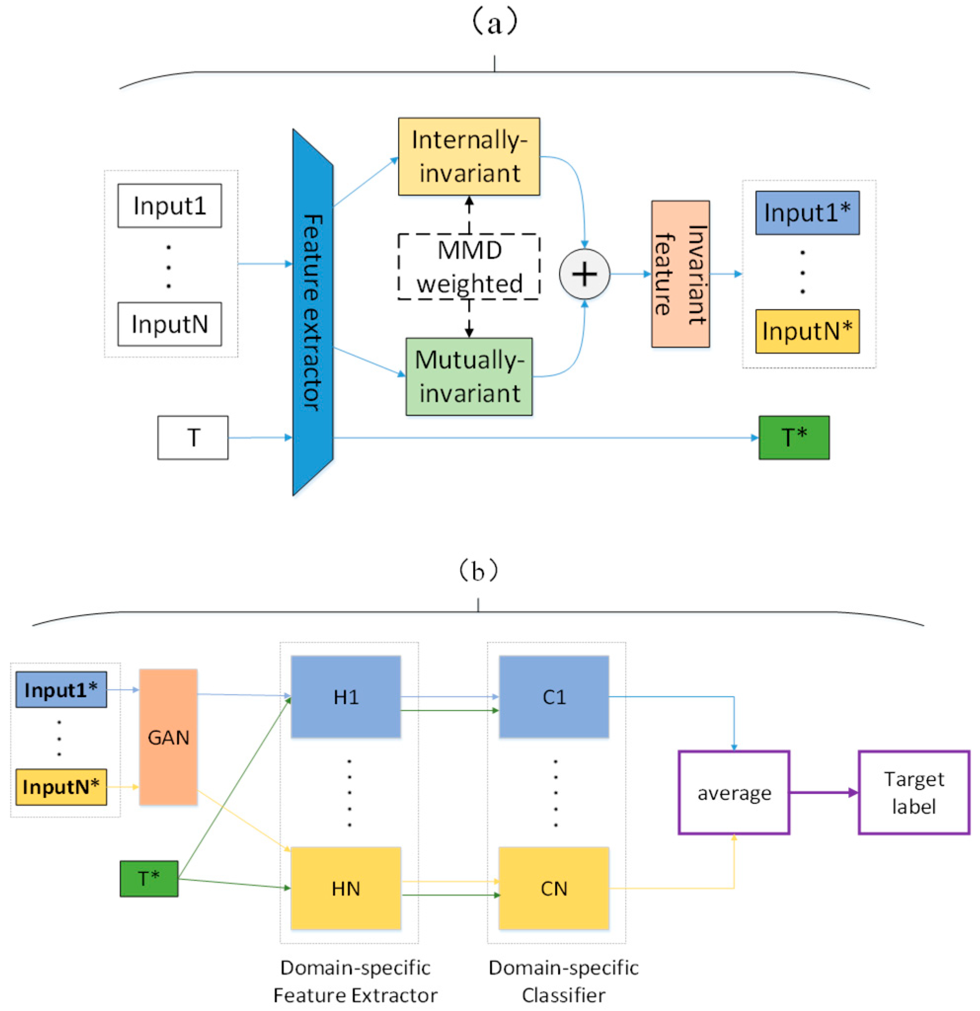
2.2. Algorithm Overview

The inherent ambiguity in HSI data boundaries can lead to an unclear representation of the source domain features, potentially resulting in the misclassification of target domain samples during the transfer process. To effectively address this challenge and accurately capture the invariant features of the source domain data, a multi-source domain boundary reinforcement self-adaptive network (MDSNI) based on invariant features is proposed herein, ensuring the precise classification of the target domain data. The MDSNI network comprises two primary stages: first, the acquisition of domain-invariant representations from multiple source domains (Figure 1a); second, the reinforcement of the source domain boundaries by aligning the source–target domains via multiclassifiers for target domain classification (Figure 1b). Our framework consists of a domain-invariant feature extractor, a GAN boundary enhancer, and specific N classifiers.

A method for acquiring the intraclass and interclass invariant features of the source domain is applied in this work, as demonstrated in Figure 1a. This method relies on distance-weighted Fourier phase information and the alignment of second-order statistics via CORAL. Our methodology takes data input from multiple source domains and uses a shared feature extractor to preprocess each source domain’s input data. The intraclass invariant features of the source domain are built based on the captured Fourier phase information. Meanwhile, the interclass invariant features of the source domain are established by calculating the second-order statistics, aligned via CORAL. Consequently, a comprehensive feature representation, encompassing multiple source domain-invariant features, is assembled by integrating these calculations via a methodology weighted using the MMD distance. This feature representation considers the characteristics of each source domain and preserves the differences between the source domains. Hence, it can provide a more accurate and resilient foundation of features to support subsequent classification tasks.

Figure 1b shows a boundary-constraint adversarial network, designed to further constrain source domain data by generating synthetic samples within the feature space. By analyzing the intraclass sample density of the source domain data with invariant features, the intraclass sample boundaries are determined. The target function of the sample density-constrained GAN is adjusted to generate samples in the source domain boundary area, thus strengthening the source domain feature space boundaries and further enhancing the source domain feature space stability. Finally, each pair of source–target domain data is mapped to multiple different feature spaces, and the distributions of specific domains are aligned to acquire multiple domain-invariant representations. Then, multiple specific domain classifiers are trained using multiple domain-invariant representations. The knowledge distillation concept and the ratio of classification errors to correct as the temperature, are leveraged to construct weighted softmax values. This approach enhances the classification accuracy of the domain classifier for the target domain.

The loss of our methodology consists of two parts: domain-invariant feature extraction loss $L_{FFT}$ and boundary-enhanced classification loss $L_{GAN}$. In particular, intraclass and interclass invariant features can be accurately extracted from multi-source domain data by minimizing the domain-invariant feature extraction loss. The network can accurately classify the target domain data by minimizing the boundary enhancement classification loss. The overall loss equation is as follows:

$$L_{loss}=L_{FFT}+\lambda L_{GAN}$$

(1)

where $\lambda$ is the hyperparameter that determines the weight between the domain-invariant feature extraction loss $L_{FFT}$ and the boundary-enhanced classification loss $L_{GAN}$.

2.3. Source Domain-Invariant Feature Extraction Based on a Weighted Fourier Transform

The domain-generalized intraclass invariant features are acquired via distance-weighted Fourier phase transformations and domain-generalized interclass invariant features via CORAL alignment. As shown in Figure 1a, the structure takes input from multiple source domains. It calculates the Fourier phase, CORAL-aligned second-order statistics, and MMD distance for each source domain upon passing through the shared feature extractor. Subsequently, multi-source domain-invariant features are constructed based on a distance weighting rule.

2.3.1. Learning Intraclass Invariant Features

Existing research [38,39,40,41,42] has noted that the Fourier phase signal retains the most high-level semantic information from the original data and is not easily affected by related data interference. Hence, the Fourier phase features of the original data can be utilized as intraclass invariant features of the domain.

The network takes the Fourier phase information and class labels as the input and output, respectively, to obtain the Fourier phase information features for classification. According to reference [43], the Fourier transform equation for single-channel two-dimensional data is as follows:

$$F\left(x\right)\left(u,v\right)={\displaystyle \sum _{h=1}^{H-1}{\displaystyle \sum _{w=0}^{W-1}x\left(h,w\right)}}•e^{-j2\pi \left(\frac{h}{H}u+\frac{w}{W}v\right)}$$

(2)

where $\left(u,v\right)$ is the index. H and W are the height and width, respectively. Then, the phase component [42] is expressed as follows:

$$P\left(x\right)=\arctan \frac{I\left(x\right)}{R\left(x\right)}$$

(3)

where $R\left(x\right)$ and $I\left(x\right)$ denote the real and imaginary parts of $F\left(x\right)$, respectively. The Fourier phase of $x$ is denoted as $x^{\prime }$, and then, the network is trained using $\left(x^{\prime },y\right)$:

$$\underset{}{L_{fft}=\underset{{\theta }^f}{\min }}{E}_{\left(x,y\right)}{L}_{cls}\left(G^f\left(x_k{}^{\prime }\right),y\right)\times \frac{1}{N-1}{\displaystyle \sum _{n=1}^{N-1}{d}_{mmd}\left(S_i,S_j\right),}i\ne j$$

(4)

where ${\theta }^f$ is the learnable parameter of the feature extractor $G^f$ in the network. E denotes the expectation, $L_{cls}$ is the cross-entropy loss, and ${\displaystyle \sum d}$ computes the MMD distance between the current source domain and the other source domains.

2.3.2. Exploring Interclass Invariant Features

As previously mentioned, the Fourier phase feature is the sole means of obtaining the intrinsic invariant features of the source domain. Hence, the interclass invariant features are explored by harnessing the cross-domain knowledge derived from multiple source domains. The following second-order statistics from CORAL alignment [8] are adopted for two domains, $S_i$ and $S_j$, to accomplish this:

$$\begin{array}{l}{L}_{coral}={{\displaystyle \sum _{i\ne j}^N\Vert C_i-C_j\Vert }}_F^2\times \frac{1}{d_{mmd}\left(S_i,S_j\right)}\left[1-\frac{S_i\cap S_j}{S_i\cup S_j}\right]\\ C_i=\frac{1}{n_i-1}\left(X^i{}^T{X}^i-\frac{1}{n_i}{\left(1^T{X}^i\right)}^T\left(1^T{X}^i\right)\right)\end{array}$$

(5)

where ${\Vert ·\Vert }_F$ denotes the Frobenius matrix paradigm, $d_{mmd}$ calculates the distance between two source domains, and the Jaccard index gives the probabilistic logical value of the correlation between the two domains.

2.4. Target Domain Classification Based on Feature Space Boundary Enhancement

Existing multi-source unsupervised domain adaptation (MUDA) methodologies predominantly concentrate on acquiring a shared domain-invariant representation that encompasses all the domains. Nevertheless, these methodologies do not fully consider the specificity of the source domain. Although invariant feature extraction can reduce data edge blurring and further enhance the intraclass structure, the presence of outliers in the source domain may cause boundary blurring of the source domain during transfer, as shown in Figure 2b. Consequently, different classifiers may predict different labels for a specific target sample in a particular domain. A new solution framework is proposed to address these challenges. For this purpose, a GAN is established to enhance the representation of the boundary data in the source domain, as shown in Figure 2c. Subsequently, the classifier’s output is aligned with the target sample to improve the classification accuracy and consistency.

2.4.1. Domain Boundary Reinforcement

The objective function of the sample density-constrained GAN generates samples in the boundary region of the source domain, thus reinforcing the known sample boundaries. The MMD serves as a measure of the difference between each source domain and target domain.

This work integrates the density peak clustering algorithm [44], using the values from the prelogit layer as the sample points to calculate the sample density at any position in the sample feature space. This information is pivotal in determining the sample boundaries. The boundary samples are generated via the GAN to strengthen the domain boundary data, generating samples around the known class boundaries. Hence, it amends the original GAN objective function in this work [22]. The modified objective function is as follows:

$$\underset{G}{\min } \underset{D}{\max }\underset{(a)}{\underbrace{E_{P_{\mathrm{kkc}}(x)}\log D(x)+E_{P_G(x)}[\log (1-D(x)]}}+\underset{(b)}{\underbrace{\beta E_{P_G(x)}[\varphi (x)]}}$$

(6)

where $\beta >0$ is a balancing parameter. When $\beta =0$, the trained classifier becomes a class classifier. This objective function is explained in two parts. The first term (a) corresponds to the original GAN loss, making the samples generated via the generator as similar as possible to the real samples. The second term (b) calculates the sample density. During the training phase, the generator and discriminator are trained multiple times under the sample density constraint, eventually leading the generator to produce low-density boundary samples, thereby enhancing the sample boundary.

The Maximum Mean Discrepancy (MMD) [45] is selected as our estimation of the difference between the two domains. The MMD estimates the distance as follows:

$$D_{\mathrm{H}}\left(p,q\right)=\Vert \frac{1}{n_s}{\displaystyle \sum _{x_i\in D_s}\varphi \left(x_i\right)}-\frac{1}{n_t}{\displaystyle \sum _{x_j\in D_t}\varphi \left(x_j\right)}\Vert$$

(7)

where $D_{\mathrm{H}}\left(p,q\right)$ is the unbiased estimator of the MMD distance between the source domain and target domain. Equation (7) is utilized as an estimate of the difference between each source domain and target domain to achieve source–target domain alignment. The MMD loss is written as follows:

$$L_{mmd}=\frac{1}{N}{\displaystyle \sum _{j=1}^{N}D\left(H_j\left(F\left(X_{sj}^{{}^{\prime }}\right)\right),H_j\left(F\left(X_t\right)\right)\right)}$$

(8)

where $X_{sj}^{{}^{\prime }}$ represents the source domain data after boundary reinforcement, as shown in Figure 2c.

2.4.2. Domain-Specific Classifier Alignment

In an ideal scenario, each classifier should yield consistent prediction outputs for the same target sample. Nevertheless, disparities in the predictions for the target samples can emerge since the classifiers are independently trained across multiple source domains in practice. This discrepancy is especially notable for target samples positioned near class boundaries, where the possibility of misclassification increases.

Hence, this section mainly accomplishes the minimization of the differences between all the classifiers. In this context, the principle of knowledge distillation is employed, using the ratio of misclassification to correct classification as the temperature to create a weighted softmax value. The difference loss is then formulated using the absolute value of the difference between the weighted softmax values for all the correctly classified target domain data:

$$L_{disc}=\frac{2}{N\times (N-1)}\sum _{j=1}^{N-1}\sum _{i=j+1}^N{E}_{x\leftrightarrow X_i}\Vert P_i-P_j\Vert$$

(9)

$$p_i=\frac{\exp (H_i\left(F\left(x\right)\right)/T)}{{\displaystyle {\sum }_k^N\exp (H_k\left(F\left(x\right)\right)/T)}},T=\frac{C_{\mathrm{error}}}{C_{\mathrm{Correct}}}$$

(10)

Each specific feature extractor can align with each pair of source domain and target domain spaces by minimizing Equation (9), thereby achieving the accurate classification of the target domain.

In summary, the following expression can be obtained after optimization:

$$L_{loss}=L_{fft}+\alpha L_{coral}+{\lambda }_1{L}_{mmd}+{\lambda }_2{L}_{disc}$$

(11)

$\alpha ,{\lambda }_1,{\lambda }_2$ are hyperparameters. Equation (11) encapsulates four objectives: (1) intraclass invariant feature learning; (2) interclass invariant feature learning; (3) boundary enhancement; and (4) classification.

The initial two objectives revolve around the acquisition of invariant representations for domain generalization, while the latter two objectives are associated with boundary enhancement and MUDA classification.

In real-world applications, the primary focus is on tuning the hyperparameters to balance these four terms. Future work will involve developing more heuristic approaches for automatically determining the hyperparameters.

3. Experiments

Furthermore, the relevant experiments are conducted on both the RGB image dataset and the hyperspectral dataset to verify the effectiveness of the MDSNI algorithm.

3.1. Target Domain Classification Based on Feature Space Boundary Enhancement

The Office-31, Office-Home, and ImageCLEF-DA public datasets are utilized to validate the RGB image dataset classification task. Office-31 [46] notably includes a total of 4652 images from three different domains, including 31 categories. Each learning task has 31 classes in the source domain and 10 classes in the target domain. Office-Home [47] includes a total of 15,588 images from four different domains, including 65 categories. Each learning task has 65 classes in the source domain and 25 classes in the target domain. ImageCLEF-DA is composed of 12 common categories shared by three public datasets, with 50 images per category and 600 images per domain.

In the experiments, the MDSNI is compared with the deep MUDA methodology Deep Cocktail Network (DCTN) [6] and MFSAN [48]. Furthermore, the MDSNI is also compared with various SUDA methodologies, including ResNet [49], Deep Domain Confusion (DDC) [27], the Deep Adaptive Network (DAN) [26], Deep CORAL (D-CORAL) [8], Reverse Gradient (RevGrad) [50], and the Residual Transfer Network (RTN) [51].

All the algorithms are fine-tuned using the ResNet model [49]. The stochastic gradient descent (SGD) with a momentum of 0.9 and the learning rate annealing strategy are incorporated into RevGrad. Moreover, ${\eta }_p=\frac{{\eta }_0}{{\left(1+\alpha \zeta \right)}^{\beta }}$ is utilized for the adjustment during the SGD, where $\zeta$ is the training progress changing linearly from 0 to 1, ${\eta }_0=0.01,\alpha =10,\beta =0.75$, which is optimized to promote convergence and low error in the source domain. To suppress noise activation in the early stages of training, the adaptation factors $\lambda$ and $\gamma$ are not determined, but gradually changed from 0 to 1 in a progressive schedule: ${\gamma }_{\zeta }={\lambda }_{\zeta }=\frac{2}{\exp \left(-\theta \zeta \right)}-1$. Moreover, $\theta =10$ is kept constant throughout the experiments.

In addition, the MDSNI is compared with the other algorithms for three datasets, and the results are presented in

Table 1. Classification accuracy (%) using the Office-31 dataset. Display the most data in bold.

Method	A, W→D	A, D→W	A, D→W	Avg
ResNet	98.31	95.73	61.88	85.34
DDC	97.22	94.05	66.73	86.03
DAN	98.60	96.82	66.92	87.42
D-CORAL	98.31	97.02	66.43	87.22
RevGrad	98.70	97.12	66.92	87.62
RTN	98.41	95.83	65.54	86.63
DCTN	98.31	97.22	63.56	86.33
MFSAN	98.51	97.52	71.97	89.30
MDSNI	99.70	99.20	73.80	91.60

,

Table 2. Classification accuracy (%) using the ImageCLEF-DA dataset. Display the most data in bold.

Method	I, C→P	I, P→C	P, C→I	Avg
ResNet	74.05	90.59	83.06	82.57
DDC	77.81	90.19	84.84	82.96
DAN	76.82	92.37	91.28	86.82
D-CORAL	76.33	92.66	90.78	86.63
RevGrad	77.12	92.76	90.88	86.92
RTN	77.81	94.35	86.03	85.04
DCTN	74.25	94.74	89.40	86.13
MFSAN	78.31	94.45	92.66	88.51
MDSNI	79.90	96.36	94.55	90.30

and

Table 3. Classification accuracy (%) using the Office-Home dataset. Display the most data in bold.

Method	C, P, R→A	A, P, R→C	A, C, R→P	A, C, P→R	Avg
ResNet	64.65	49.10	78.90	74.65	66.83
DDC	63.46	50.29	77.42	74.25	66.33
DAN	67.82	88.51	78.21	81.68	71.68
D-CORAL	67.42	58.01	78.71	81.87	71.48
RevGrad	67.72	58.51	78.71	81.87	71.68
MFSAN	71.38	61.38	79.50	80.98	73.36
MDSNI	72.83	62.63	81.11	82.63	74.85

, respectively.

The following conclusions can be drawn based on the analysis of the above results.

The MDSNI demonstrates superior performance over all the compared methodologies across most multi-source transfer tasks. This underscores the significance of the domain-invariant feature construction algorithm introduced in this work and the enhancement of specific class boundaries.

Comparatively, the results achieved using the MDSNI methodology in the experiments surpass those of the MUDA methodology, DCTN. The analysis suggests that this is mainly because the MDSNI extracts domain-invariant feature representations from multiple source domains. It effectively discriminates between the information for each source domain, resulting in a more robust generalization of the source domain knowledge to unknown target domains. The DCTN lacks consideration of the boundary ambiguity of multiple source domains when extracting features, which makes it challenging for the classifier to adapt to the variations between each source domain. In contrast, the MDSNI excels in capturing shared knowledge across different source domains by acquiring domain-invariant representation in the feature space of each source domain. The experimental results also show that the MDSNI outperforms the MFSAN, which indicates that the source domain boundaries can be enhanced by constraining the GAN to generate fake samples in the feature space and construct domain-specific decision boundaries, ultimately enhancing the target domain’s classification accuracy.

Compared with SUDA methodologies like DAN (source combine), the MDSNI stands out for its ability to extract multiple domain invariant representations within multiple feature spaces. In contrast, DAN focuses on extracting common domain-invariant representations within a shared feature space. The superior performance of the MDSNI over DAN (source combine) suggests that extracting a single common domain-invariant representation from all domains can be challenging.

Figure 3 visualizes the tasks learned via DAN (single source) for D→A, the tasks learned via MFSAN for D, W→A, and the tasks learned via MDSNI for D, W→A using t-SNE embeddings. The results in Figure 3b surpass those in Figure 3a, indicating the benefits of considering multiple source domains. Furthermore, the results in Figure 3c outperform those in Figure 3b, further affirming the effectiveness of our model in adapting specific domain distributions and classifiers.

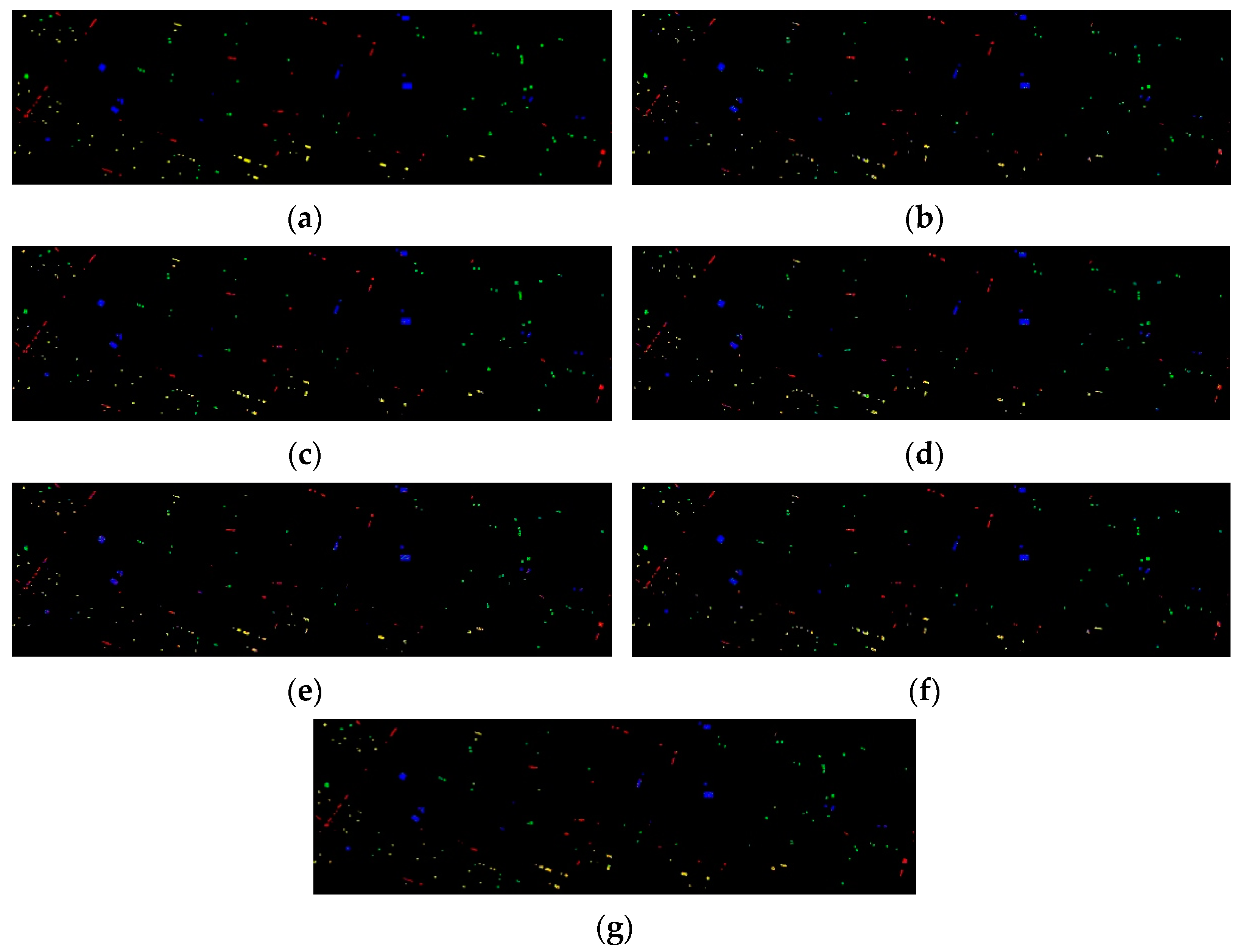
3.2. HSI Image Dataset Classification Task

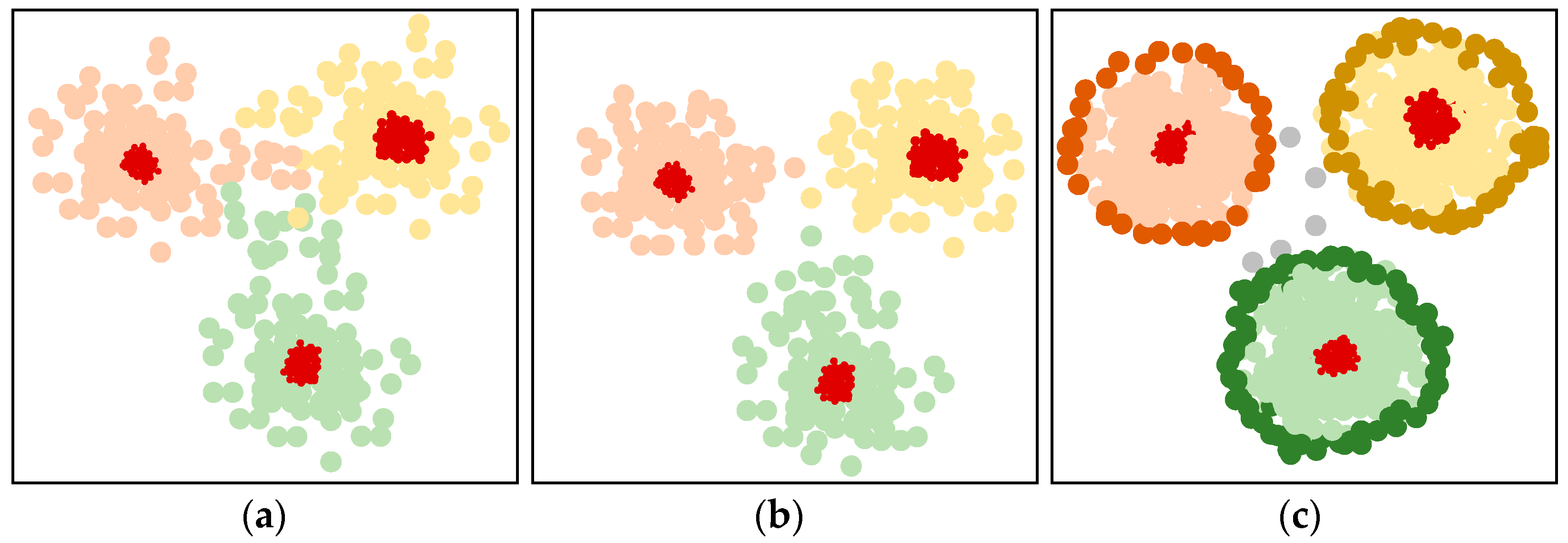
3.2.1. Invariant Feature Network Performance Analysis

The performance of invariant feature networks is assessed using the Pavia University, Pavia Center, and Salinas Valley datasets. The Pavia University dataset comprises 103 effective spectral bands, encompassing nine land-use categories for classification. Similarly, the Pavia Center dataset consists of 102 spectral bands, representing nine land-use targets. The Salinas Valley dataset offers 204 spectral bands, with 16 diverse land-use categories designated for classification.

For the sample partitioning procedures, the samples are initially randomized within each category. Subsequently, r% of the samples (r = 40, 50, 60, 70) are selected from each category and assigned their true class labels to form a training set; 30% of the samples will be utilized as the test set. These experimental procedures should be repeated five times to mitigate the influence of edge effects stemming from random sampling and ensure the reliability of our experiment. Then, the classification results are averaged to assess the performance of the algorithm. The network training setup remains consistent with that outlined in Section 3.1.

In this section, the algorithm proposed in this work is compared with the SVM algorithm based on spectral-extended morphological attribute profile joint feature representation [52] (Spe-EMAP SVM), a stacked autoencoder based on spectral–spatial joint feature representation [1] (JSSAE), a stacked sparse autoencoder based on spectral features (Spe-SSAE), a stacked sparse autoencoder based on extended morphological attribute profile features (EMAP-SSAE), and a stacked sparse autoencoder based on spectral-extended morphological attribute profile joint feature representation (Spe-EMAP SSAE).

Table 4. Overall classification accuracy of different classification methods at Pavia University. Display the most data in bold.

Training Sample Rate	Spe-EMAP SVM	JS SAE	Spe-SSAE	EMAP-SSAE	Spe-EMAP SSAE	MDSNI
40%	93.66%	91.93%	90.85%	98.05%	98.76%	99.29%
50%	94.58%	92.64%	91.43%	98.30%	98.85%	99.52%
60%	95.01%	92.83%	91.58%	98.43%	98.94%	99.47%
70%	95.36%	93.64%	92.28%	98.62%	99.06%	99.54%

,

Table 5. Overall classification accuracy of different classification methods at Pavia Centre. Display the most data in bold.

Training Sample Rate	Spe-EMAP SVM	JS SAE	Spe-SSAE	EMAP-SSAE	Spe-EMAP SSAE	MDSNI
40%	98.77%	98.38%	99.27%	99.42%	99.69%	99.29%
50%	99.04%	98.55%	99.34%	99.69%	99.79%	99.52%
60%	99.10%	98.64%	99.46%	99.74%	99.85%	99.47%
70%	99.16%	98.73%	99.62%	99.76%	99.87%	99.54%

and

Table 6. Overall classification accuracy of different classification methods at Salinas Valley. Display the most data in bold.

Training Sample Rate	Spe-EMAP SVM	JS SAE	Spe-SSAE	EMAP-SSAE	Spe-EMAP SSAE	MDSNI
40%	93.11%	90.89%	89.23%	96.12%	96.82%	97.46%
50%	94.07%	91.72%	89.43%	96.23%	96.93%	97.68%
60%	94.72%	91.81%	89.48%	96.59%	97.00%	97.90%
70%	95.11%	92.36%	89.71%	96.76%	97.11%	98.06%

present the corresponding results from these comparisons. Figure 4, Figure 5 and Figure 6 depict the classification outcomes achieved using various methodologies across three HIS databases.

The proposed MDSNI algorithm exhibits exceptional classification performance during the experiments. Among the six algorithms tested, MDSNI stands out by achieving the highest accuracy in completing the classification task.

It is worth noting that when training support vector machine (SVM) and stacked sparse self-encoder (SSAE) classification models with the same set of features, SSAE consistently outperforms SVM in terms of overall classification accuracy. This observation further underscores the advantages of deep features in enhancing stability and robustness, emphasizing the significant improvement that deep features bring to the classification performance using hyperspectral images.

A comparison of the actual classification results reveals that our methodology outperforms other methodologies in reducing misclassified pixels. This achievement can be primarily attributed to the constructed domain-invariant feature extraction algorithm, which effectively harnesses the spectral and spatial information of the hyperspectral images to improve classification accuracy. Substantial classification errors are found in certain regions with the application of SVM and SSAE when examining the Salinas Valley dataset and comparing it with the ground truth. In contrast, the MDSNI primarily exhibits sporadic misclassifications. This notable difference can be primarily attributed to the intraclass invariant and interclass invariant feature structures, based on the Fourier phase information and CORAL correlation-aligned second-order statistics proposed using the MDSNI, and the invariant features weighted and enhanced according to the MMD distance. Additionally, the adversarial network, which is founded on boundary constraints and introduced via the MDSNI, constrains the source domain data by generating spurious samples in the feature space. The generation of synthetic samples in the feature space via the GAN enhances the reliability and richness of the feature space, consequently fortifying the feature space boundaries. These findings collectively underscore the substantial advantages of our proposed MDSNI network in improving classification performance.

Finally, our experimental results consistently underscore the exceptional performance of our method. Even when maintaining a constant training rate, the MDSNI algorithm shows significant advantages over the other methodologies, proving its superior performance in extracting intraclass and interclass invariant features in multi-source domains. When the training rate is increased from 60 to 70%, the classification results of the MDSNI algorithm display minimal variation despite the augmented volume of the training data. This observation illustrates the capability of our methodology to yield favorable outcomes, even with relatively limited training data. Such stable performance augments the practical applicability of our approach.

Table 7. Comparison of MDSNI with the latest HIS unsupervised classification algorithm. Display the most data in bold.

Method	Pavia University	Pavia Center	Salinas Valley
MDSNI	99.23%	99.54%	98.06%
PSSA [53]	97.92%	97.49%	95.12%
Diff-HIS [54]	96.38%	96.53%	96.10%

shows the comparison between our algorithm and the latest HIS unsupervised classification algorithm. During the sample classification, it first randomizes the samples within each category and then selects 70% of the samples from each category to give them the true class label, forming the training sample set. On the other hand, 30% of the samples will be utilized as the test sample set. The following experimental operations are repeated five times to mitigate potential edge effects caused by random sampling and to ensure the reliability of the experiments. Subsequently, the algorithm performance is assessed by computing the average of the classification results. The network training settings are the same as those in Section 3.1.

In our experiments, the performance of the MDSNI is compared with that of the PSSA and Diff-HIS algorithms in the HSI classification task. The results show that the MDSNI algorithm outperforms the PSSA and Diff-HIS algorithms, and this superiority mainly stems from the unique advantages to our approach in utilizing invariant features and establishing robust boundary strategies.

The MDSNI constructs a boundary constraint-based adversarial network, which reinforces the boundary in the source domain-invariant feature space by generating fake samples to populate the source domain-invariant feature space. In contrast, Diff-HIS simply uses an unlabeled HSI patch pretrained diffusion model for unsupervised feature learning and then exploits intermediate-level features with various time steps for classification. The PSSA combines entropy rate superpixel segmentation (ERS), superpixel-based principal component analysis (PCA), and PCA-domain two-dimensional singularity spectral analysis (SSA) to enhance the feature extraction efficacy and efficiency, combined with anchor-based graph clustering (AGC) for effective classification. Nevertheless, both methodologies fail to consider the ambiguity of the edges in the HSI data, which makes the possibility of classification error of the edge data extremely high when classifying HSI data, resulting in a lower classification accuracy than that of the MDSNI.

In summary, the excellent performance of our MDSNI algorithm mainly stems from its accurate invariant feature extraction and robust boundary reinforcement strategy. These two points enable the MDSNI to markedly improve the classification accuracy when performing HSI classification tasks, thus making its overall performance superior to other competing algorithms.

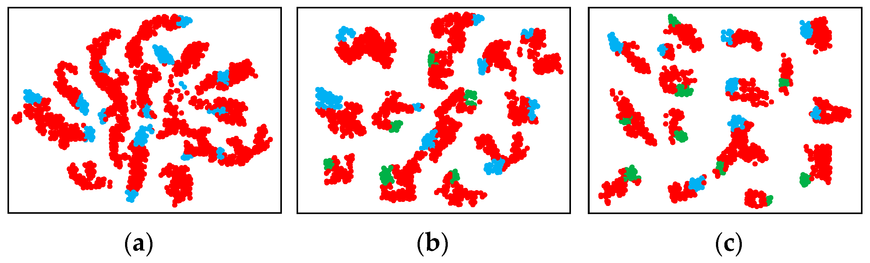
3.2.2. Performance Analysis of the MUDA Sample Transfer Algorithm

To assess the effectiveness of the methodology introduced in this chapter for hyperspectral image transfer classification, experiments are conducted employing three datasets: Pavia University (PU), Houston (H), and Washington DC Mall (W). The Houston dataset includes a total of 144 bands, with a spatial resolution of 2.5 m. The Washington DC Mall dataset comprises 305 × 280 pixels and 191 bands. Four specific types of features are selected as transfer targets for all three datasets in the experimental process. These four types of features are roads, grasslands, trees, and roofs. The pseudocolor images and ground realities for the three datasets are shown in Figure 7.

Drawing from the aforementioned hyperspectral remote sensing datasets, two groups of data are selected as the source domain and the remaining group as the target domain to create cross-domain multi-source experimental data for verification. Throughout the experimental process, the MDSNI is compared with the SVM, 3D-SAE [55], Deep CORAL, DAN, and UHDAC to demonstrate the superiority of the proposed methodology. The learning settings mirrored those utilized in Section 3.1.

In the results analysis stage, the overall classification accuracy (OA) and the kappa coefficient are utilized as evaluation indicators to compare the experimental results; each experiment is repeated ten times, and the average value is taken. The experimental results are presented in

Table 8. Comparison of hyperspectral image classification results (PU, W→H). Display the most data in bold.

	Road (%)	Grass (%)	Tree (%)	Roofs (%)	OA (%)	Kappa
SVM	73.73	76.18	60.47	54.95	66.28	0.5494
3D-SAE	76.94	79.08	68.81	67.33	73.01	0.6398
Deep CORAL	77.88	82.22	71.84	67.21	74.7	0.6627
DAN	79.72	85.9	75.49	76.04	79.6	0.7275
UHDAC	81.89	98.53	72.56	81.08	83.94	0.7856
MDSNI	88.53	89.93	83.67	81.29	85.85	0.8111

and

Table 9. Comparison of hyperspectral image classification results (PU, H→W). Display the most data in bold.

	Road (%)	Grass (%)	Tree (%)	Roofs (%)	OA (%)	Kappa
SVM	71.16	79.74	63.63	68.3	68.43	0.5731
3D-SAE	75.87	85.52	69.43	71.86	74.9	0.6561
Deep CORAL	80.35	85.02	73.31	75.33	77.99	0.6971
DAN	85.86	86.41	76.59	79.21	81.65	0.7466
UHDAC	83.13	93.49	84.84	83.09	85.4	0.7988
MDSNI	87.56	93.15	86.18	85.3	87.41	0.8266

. Figure 8 and Figure 9 show the classification results for the HIS data transfer learning.

The analysis reveals the following.

Traditional hyperspectral image classification algorithms, such as SVM and 3D-SAE, only consider the source domain data during training and fail to consider the relationship between the source domain and the target domain; thus, they perform poorly on the target domain classification task, resulting in low overall accuracy and kappa coefficient. In contrast, transfer learning algorithms, such as the MDSNI, UHDAC, DAN, and Deep CORAL, utilize the features of both the source and target domains during the training process. Moreover, these transfer learning algorithms are designed to mitigate the distributional differences between the source and target domains, ultimately enhancing the classification performance in the target domain. For instance, the MDSNI effectively captures the internal and interval invariant feature structure of the source and target domains by incorporating the Fourier phase information and CORAL correlation-aligned second-order statistics. The UHDAC improves the domain adaptation using an unsupervised hierarchical deep clustering approach, facilitating the learning on the shared and specific features of the source and target domains. In a similar vein, DAN and Deep CORAL bolster the domain adaptability by maximizing the similarity between the feature distributions in the source and target domains, thereby reducing the distributional differences between the domains. The overarching objective of these methodologies is to leverage information from both the source and target domains during training to achieve better classification performance on the target domain. As a result, they significantly outperform traditional hyperspectral image classification algorithms, such as SVM and 3D-SAE, when it comes to the target domain classification task, which improves the overall accuracy and kappa coefficient.

The transfer learning algorithms, Deep CORAL and DAN, aim to mitigate the disparity in domain distribution between the source and target domains by introducing domain adaptation layers. Nevertheless, Deep CORAL incorporates fewer domain adaptation layers, which limits its effectiveness when handling hyperspectral data. In addition, Deep CORAL and DAN are implemented without considering the problem of fuzzy boundaries between the source and target domain data. Consequently, their accuracy and kappa coefficient in hyperspectral image classification tasks are lower than those of the MDSNI.

The UHDAC strives to establish consistent feature mapping between the source and target domains and align the data distributions of the two domains via bidirectional adversarial migration. Nevertheless, the UHDAC tends to overlook the invariant features of the source domain, which results in its performance in hyperspectral experiments slightly lagging behind that of the MDSNI. While 3D-SAE combines the features of both the source and target domains for hyperspectral images and extracts the spatial–spectral features, its limited performance leads to the inaccurate representation of the edge information for the hyperspectral images from different domains. Consequently, the parameters of the network trained on the source domain data cannot be directly adapted to the training of the target domain data. This difference in performance manifests as the accuracy and kappa coefficient of the MDSNI methodology significantly outperforming those of the 3D-SAE.

Our algorithm notably excels and attains the desired classification results, even in the presence of substantial disparities in the sample data distribution between the source and target domains. This robustly underscores the effectiveness of our approach in addressing discrepancies in data distribution between source and target domains.

The extensive array of experimental results underscores the substantial advantages of our MDSNI method compared to state-of-the-art transfer learning techniques using widely available benchmark datasets. Our methodology consistently delivers high-quality image classification results for the target domain, despite the presence of data distribution inconsistencies between the source and target domains. This is consistently confirmed across multiple experiments, affirming the broad potential applicability of our methodology in dealing with the hyperspectral image classification task in real-world scenarios.

4. Conclusions

In this work, an MDSNI is introduced for hyperspectral image classification. Leveraging principles from deep learning and transfer learning, the MDSNI addresses the challenge of domain adaptation that previous methodologies may have overlooked, resulting in significant enhancements in classification accuracy and model generalization.

The MDSNI leverages MMD distance-weighted Fourier phase information to capture intraclass invariant features and employs interclass invariant features via the relevance-weighted CORAL alignment of second-order statistics. Furthermore, the source domain boundary and the construction of multiple domain classifiers are bolstered by integrating a GAN. This strategy allows us to align the domain-specific distributions between each pair of source and target domains, ultimately facilitating the precise classification of the target domain.

Our experiments have demonstrated that our proposed MDSNI methodology exhibits robust performance, even in the presence of significant discrepancies in the sample data distributions between the source and target domains. This highlights the effectiveness of our approach in addressing inconsistencies in the distributions of source and target domain data.

In conclusion, our extensive experimental results on public benchmark datasets show that our proposed algorithm has significantly improved the multi-source unsupervised domain adaptation (MUDA) methodology, outperforming leading-edge methodologies. This research significantly contributes to the field of hyperspectral image classification and holds promise for further advancements in the domain of remote sensing.

It is worth noting that, while this work employs a basic density methodology to determine the source domain boundary, real-world data distributions often exhibit considerable diversity. Some data distributions are inherently tight. Given this variability, the existing density methodology may not be able to completely and accurately depict the source domain boundary. Therefore, future research will focus on finding more adaptable boundary judgment algorithms.

References

1. Chen, Y.; Lin, Z.; Xing, Z.; Wang, G.; Gu, Y. Deep learning-based classification of hyperspectral data. IEEE J. Sel. Top. Appl. Earth Obs. Remote Sens. 2017, 7, 2094–2107. [Google Scholar] [CrossRef]
2. Wang, J.; Lan, C.; Liu, C.; Ouyang, Y.; Qin, T.; Lu, W.; Chen, Y.; Zeng, W.; Yu, P. Generalizing to unseen domains: A survey on domain generalization. IEEE Trans. Knowl. Data Eng. 2022, 8, 8052–8072. [Google Scholar] [CrossRef]
3. Pan, S.J.; Yang, Q. A survey on transfer learning. IEEE Trans. Knowl. Data Eng. (TKDE) 2010, 22, 1345–1359. [Google Scholar] [CrossRef]
4. Xia, M.; Yuan, G.; Yang, L.; Xia, K.; Ren, Y.; Shi, Z.; Zhou, H. Few-Shot Hyperspectral Image Classification Based on Convolutional Residuals and SAM Siamese Networks. Electronics 2023, 12, 3415. [Google Scholar] [CrossRef]
5. Huang, J.; Gretton, A.; Borgwardt, K.M.; Scholkopf, B.; Smola, A.J. Correcting sample selection bias by unlabeled data. Neural Inf. Process. Syst. 2007, 19, 601–608. [Google Scholar]
6. Jiang, J.; Zhai, C. Instance Weighting for Domain Adaptation in NLP; Association for Computational Linguistics (ACL): Prague, Czech Republic, 2007; pp. 264–271. [Google Scholar]
7. Fernando, B.; Habrard, A.; Sebban, M.; Tuytelaars, T. Unsupervised visual domain adaptation using subspace alignment. In Proceedings of the International Conference on Computer Vision (ICCV), Sydney, NSW, Australia, 1–8 December 2013; pp. 2960–2967. [Google Scholar]
8. Sun, B.; Saenko, K. Deep coral: Correlation alignment for deep domain adaptation. In Proceedings of the European Conference on Computer Vision (ECCV), Amsterdam, The Netherlands, 11–14 October 2016; pp. 443–450. [Google Scholar]
9. Long, M.; Zhu, H.; Wang, J.; Jordan, M.I. Deep transfer learning with joint adaptation networks. In Proceedings of the International Conference on Machine Learning (ICML), Sydney, NSW, Australia, 17 August 2017; pp. 2208–2217. [Google Scholar]
10. Tzeng, E.; Hoffman, J.; Saenko, K.; Darrell, T. Adversarial discriminative domain adaptation. In Proceedings of the Conference on Computer Vision and Pattern Recognition (CVPR), Honolulu, HI, USA, 21–26 July 2017; Volume 1, p. 4. [Google Scholar]
11. Hoffman, J.; Tzeng, E.; Park, T.; Zhu, J.-Y.; Isola, P.; Saenko, K.; Efros, A.A.; Darrell, T. Cycada: Cycle-consistent adversarial domain adaptation. In Proceedings of the International Conference on Machine Learning, Montreal, QC, Canada, 10–15 July 2018. [Google Scholar]
12. Xu, Y.; Kan, M.; Shan, S.; Chen, X. Mutual learning of joint and separate domain alignments for multi-source domain adaptation. In Proceedings of the IEEE/CVF Winter Conference on Applications of Computer Vision, Waikaloa, HI, USA, 15 August 2022. [Google Scholar]
13. Liu, H.; Shao, M.; Fu, Y. Structure-preserved multi-source domain adaptation. In Proceedings of the 16th International Conference on Data Mining, Barcelona, Spain, 12–15 December 2016; pp. 1059–1064. [Google Scholar]
14. Ben-David, S.; Blitzer, J.; Crammer, K.; Pereira, F. Analysis of representations for domain adaptation. In Proceedings of the Advances in Neural Information Processing Systems 19, Vancouver, BC, Canada, 4–7 December 2006. [Google Scholar]
15. Hu, J.; Lu, J.; Tan, Y.-P.; Zhou, J. Deep transfer metric learning. IEEE Trans. Image Process. 2016, 25, 5576–5588. [Google Scholar] [CrossRef] [PubMed]
16. Blitzer, J.; Crammer, K.; Kulesza, A.; Pereira, F.; Wortman, J. Learning bounds for domain adaptation. In Proceedings of the Neural Information Processing Systems 20, Vancouver, BC, Canada, 3–6 December 2008; pp. 129–136. [Google Scholar]
17. Mansour, Y.; Mohri, M.; Rostamizadeh, A. Domain adaptation with multiple sources. In Proceedings of the Neural Information Processing Systems, Vancouver, BC, Canada, 10–11 December 2009; pp. 1041–1048. [Google Scholar]
18. Xu, R.; Chen, Z.; Zuo, W.; Yan, J.; Lin, L. Deep cocktail network: Multi-source unsupervised domain adaptation with category shift. In Proceedings of the Conference on Computer Vision and Pattern Recognition, Salt Lake City, UT, USA, 18–22 June 2018; pp. 3964–3973. [Google Scholar]
19. Zhao, H.; Zhang, S.; Wu, G.; Gordon, G.J. Multiple source domain adaptation with adversarial learning. In Proceedings of the ICLR, Vancouver, BC, Canada, 15 February 2018. [Google Scholar]
20. Schlachter, P.; Liao, Y.; Yang, B. Deep One-Class Classification Using Intra-Class Splitting. In Proceedings of the 2019 IEEE Data Science Workshop (DSW), Minneapolis, MN, USA, 16 September 2019. [Google Scholar] [CrossRef]
21. Schlachter, P.; Liao, Y.; Yang, B. Open-Set Recognition Using Intra-Class Splitting. In Proceedings of the 2019 27th European Signal Processing Conference (EUSIPCO), Coruna, Spain, 2–6 September 2019. [Google Scholar] [CrossRef]
22. Li, X.; Fei, J.; Qi, Z.; Lv, Z.; Jiang, H. Open Set Recognition for Encrypted Traffic using Intra-class Partition and Boundary Sample Generation. In Proceedings of the 2022 IEEE 5th Advanced Information Management, Communicates, Electronic and Automation Control Conference (IMCEC), Chongqing, China, 16–18 December 2022; Volume 5. [Google Scholar]
23. Neal, L.; Olson, M.; Fern, X.; Wong, W.K.; Li, F. Open set learning with counterfactual images. In Proceedings of the European Conference on Computer Vision (ECCV), Munich, Germany, 8–14 September 2018. [Google Scholar]
24. Xia, Z.; Wang, P.; Dong, G. Adversarial Motorial Prototype Framework for Open Set Recognition. arXiv 2021, arXiv:2108.04225. [Google Scholar] [CrossRef]
25. Johansson, F.D.; Sontag, D.; Ranganath, R. Support and invertibility in domain-invariant representations. In Proceedings of the 22nd International Conference on Artificial Intelligence and Statistics, Okinawa, Japan, 16–18 April 2019; pp. 527–536. [Google Scholar]
26. Ben-David, S.; Blitzer, J.; Crammer, K.; Kulesza, A.; Pereira, F.; Wortman Vaughan, J. A theory of learning from different domains. Mach. Learn. 2010, 79, 151–175. [Google Scholar] [CrossRef]
27. Zhao, H.; Des Combes, R.T.; Zhang, K.; Gordon, G. On learning invariant representations for domain adaptation. In Proceedings of the International Conference on Machine Learning, Long Beach, CA, USA, 10–15 June 2019; pp. 7523–7532. [Google Scholar]
28. Li, Y.; Gong, M.; Tian, X.; Liu, T.; Tao, D. Domain generalization via conditional invariant representations. In Proceedings of the AAAI Conference on Artificial Intelligence, New Orleans, LA, USA, 29 April 2018; Volume 32. [Google Scholar]
29. Motiian, S.; Piccirilli, M.; Adjeroh, D.A.; Doretto, G. Unified deep supervised domain adaptation and generalization. In Proceedings of the IEEE International Conference on Computer Vision, Venice, Italy, 22–29 October 2017; pp. 5715–5725. [Google Scholar]
30. Ganin, Y.; Ustinova, E.; Ajakan, H.; Germain, P.; Larochelle, H.; Laviolette, F.; Marchand, M.; Lempitsky, V. Domain-adversarial training of neural networks. J. Mach. Learn. Res. 2016, 17, 2096–2130. [Google Scholar]
31. Li, Y.; Tian, X.; Gong, M.; Liu, Y.; Liu, T.; Zhang, K.; Tao, D. Deep domain generalization via conditional invariant adversarial networks. In Proceedings of the European Conference on Computer Vision (ECCV), Munich, Germany, 8–14 September 2018; pp. 624–639. [Google Scholar]
32. Rahman, M.M.; Fookes, C.; Baktashmotlagh, M.; Sridharan, S. Correlation-aware adversarial domain adaptation and generalization. Pattern Recognit. 2020, 100, 107124. [Google Scholar] [CrossRef]
33. Liu, C.; Sun, X.; Wang, J.; Tang, H.; Li, T.; Qin, T.; Chen, W.; Liu, T. Learning causal semantic representation for out-of-distribution prediction. In Proceedings of the Neural Information Processing Systems, Virtual, 6–14 December 2021. [Google Scholar]
34. Piratla, V.; Netrapalli, P.; Sarawagi, S. Efficient domain generalization via commonspecific low-rank decomposition. In Proceedings of the International Conference on Machine Learning, Virtual, 12–18 July 2020; pp. 7728–7738. [Google Scholar]
35. Hong, X.; Yong, W.; Zhi, W.; Yi, W. Embedding-based complex feature value coupling learning for detecting outliers in non-iid categorical data. In Proceedings of the AAAI Conference on Artificial Intelligence, Honolulu, HI, USA, 27 January–1 February 2019; Volume 33, pp. 5541–5548. [Google Scholar]
36. Shankar, S.; Piratla, V.; Chakrabarti, S.; Chaudhuri, S.; Jyothi, P.; Sarawagi, S. Generalizing across domains via cross-gradient training. In Proceedings of the International Conference on Learning Representations, Vancouver, BC, Canada, 30 April–3 May 2018. [Google Scholar]
37. Balaji, Y.; Sankaranarayanan, S.; Chellappa, R. Metareg: Towards domain generalization using me-ta-regularization. Adv. Neural Inf. Process. Syst. 2018, 31, 998–1008. [Google Scholar]
38. Yang, Y.; Soatto, S. Fda: Fourier domain adaptation for semantic segmentation. In Proceedings of the IEEE/CVF Conference on Computer Vision and Pattern Recognition, Seattle, WA, USA, 13–19 June 2020; pp. 4085–4095. [Google Scholar]
39. Yang, Y.; Lao, D.; Sundaramoorthi, G.; Soatto, S. Phase consistent ecological domain adaptation. In Proceedings of the IEEE/CVF Conference on Computer Vision and Pattern Recognition, Seattle, WA, USA, 13–19 June 2020; pp. 9011–9020. [Google Scholar]
40. Nussbaumer, H.J. The fast fourier transform. In Fast Fourier Transform and Convolution Algorithms; Springer: Berlin/Heidelberg, Germany, 1981; pp. 80–111. [Google Scholar]
41. Oppenheim, A.; Lim, J.; Kopec, G.; Pohlig, S.C. Phase in speech and pictures. In Proceedings of the ICASSP’79 IEEE International Conference on Acoustics, Speech, and Signal Processing, Washington, DC, USA, 2–4 April 1979; Volume 4, pp. 632–637. [Google Scholar]
42. Oppenheim, A.V.; Lim, J.S. The importance of phase in signals. Proc. IEEE 1981, 69, 529–541. [Google Scholar] [CrossRef]
43. Xu, Q.; Zhang, R.; Zhang, Y.; Wang, Y.; Tian, Q. A fourier-based framework for domain generalization. In Proceedings of the IEEE/CVF Conference on Computer Vision and Pattern Recognition, Nashville, TN, USA, 20–25 June 2021; pp. 14383–14392. [Google Scholar]
44. Rodriguez, A.; Laio, A. Clustering by fast search and find of density peaks. Science 2014, 344, 1492–1496. [Google Scholar] [CrossRef] [PubMed]
45. Gretton, K.M.; Borgwardt, M.J.; Rasch, M.J.; Schölkopf, B.; Smola, A. A kernel two-sample test. J. Mach. Learn. Res. 2012, 13, 723–773. [Google Scholar]
46. Wang, J.; Feng, W.; Chen, Y.; Yu, H.; Huang, M.; Yu, P.S. Visual domain adaptation with manifold embedded distribution alignment. In Proceedings of the ACM Multimedia Conference (MM), Amsterdam, The Netherlands, 12–15 June 2018; pp. 402–410. [Google Scholar]
47. Saenko, K.; Kulis, B.; Fritz, M.; Darrell, T. Adapting visual category models to new domains. In Proceedings of the European Conference on Computer Vision, Crete, Greece, 5–11 September 2010; pp. 213–226. [Google Scholar]
48. Zhu, Y.; Zhuang, F.; Wang, D. Aligning Domain-Specific Distribution and Classifier for Cross-Domain Classification from Multiple Sources. In Proceedings of the AAAI Conference on Artificial Intelligence, Honolulu, HI, USA, 27 January–1 February 2019; Volume 33, pp. 5989–5996. [Google Scholar]
49. He, K.; Zhang, X.; Ren, S.; Sun, J. Deep residual learning for image recognition. In Proceedings of the Computer Vision and Pattern Recognition, Las Vegas, NV, USA, 26 June–1 July 2016; pp. 770–778. [Google Scholar]
50. Ganin, Y.; Lempitsky, V. Unsupervised domain adaptation by backpropagation. In Proceedings of the International Conference on Machine Learning, Lille, France, 6–11 July 2015; pp. 1180–1189. [Google Scholar]
51. Long, M.; Zhu, H.; Wang, J.; Jordan, M.I. Unsupervised domain adaptation with residual transfer networks. In Proceedings of the Neural Information Processing Systems, Barcelona, Spain, 5–10 December 2016; pp. 136–144. [Google Scholar]
52. Fauvel, M.; Benediktsson, J.A.; Chanussot, J.; Sveinsson, J.R. Spectral and Spatial Classification of Hyperspectral Data Using SVMs and Morphological Profiles. IEEE Trans. Geosci. Remote Sens. 2008, 46, 3804–3814. [Google Scholar] [CrossRef]
53. Liu, Q.; Xue, D.; Tang, Y.; Zhao, Y.; Ren, J.; Sun, H.P. PSSA: PCA-Domain Superpixelwise Singular Spectral Analysis for Unsupervised Hyperspectral Image Classification. Remote Sens. 2023, 15, 890. [Google Scholar] [CrossRef]
54. Zhou, J.; Sheng, J.; Fan, J.; Ye, P.; He, T.; Wang, B.; Chen, T. When Hyperspectral Image Classification Meets Diffusion Models: An Unsupervised Feature Learning Framework. arXiv 2023, arXiv:2306.08964. [Google Scholar]
55. Roy, S.K.; Krishna, G.; Dubey, S.; Chaudhuri, B.B. HybridSN: Exploring 3D-2D CNN feature hierarchy for hyperspectral image classification. IEEE Geosci. Remote Sens. Lett. 2020, 17, 277–281. [Google Scholar] [CrossRef]
Figure 1. MDSNI framework. (a) Source domains invariant representation. (b) Target domain classification.
Remotesensing 15 05306 g001
Figure 2. (a) Original multi-source domain data, with blurred data edges and a high overlap rate between classes; (b) multi-source domain data after domain-invariant processing, with reduced data edge blur and a lower overlap rate between classes; (c) multi-source domain data after GAN boundary enhancement, with clear data edges and the lowest overlap rate between classes.
Remotesensing 15 05306 g002
Figure 3. The visualization of latent representations of source and target domains. (a) DAN (single source) D→A, (b) MFSAN: D, W→A, (c) MDSNI: D, W→A. Blue points represent samples from source domain D, green points represent samples from source domain W, and red points represent samples from target domain A.
Remotesensing 15 05306 g003
Figure 4. Classification results for different methods at Pavia University. (a) Ground truth. (b) Spe-EMAP SVM. (c) JSSAE. (d) Spe-SSAE. (e) EMAP-SSAE. (f) EMAP-SSAE. (g) Ours.
Remotesensing 15 05306 g004
Figure 5. Classification results for different methods at Pavia Center. (a) Ground truth. (b) Spe-EMAP SVM. (c) JSSAE. (d) Spe-SSAE. (e) EMAP-SSAE. (f) Spe-EMAP SSAE. (g) Ours.
Remotesensing 15 05306 g005
Figure 6. Classification results for different methods at Salinas Valley. (a) Ground truth. (b) Spe-EMAP SVM. (c) JSSAE. (d) Spe-SSAE. (e) EMAP-SSAE. (f) Spe-EMAP SSAE. (g) Ours.
Remotesensing 15 05306 g006
Figure 7. Pseudocolor images and ground realities for the three datasets: (a) pseudocolor image of the Pavia University dataset, (b) ground reality; (c) pseudocolor image of the Washington DC Mall dataset, (d) ground reality; (e) pseudocolor image of the Houston dataset, (f) ground reality.
Remotesensing 15 05306 g007
Figure 8. Hyperspectral image classification effect diagram (PU, W→H). (a) Ground truth. (b) SVM. (c) UHDAC. (d) DAN. (e) Deep CORAL. (f) 3D-SAE. (g) Ours.
Remotesensing 15 05306 g008
Figure 9. Hyperspectral image classification effect diagram (PU, H→W). (a) Ground truth. (b) SVM. (c) UHDAC. (d) DAN. (e) UHDAC. (f) DAN. (g) Ours.
Remotesensing 15 05306 g009