The Selection of Basic Functions for a Time-Varying Model of Unmodeled Errors in Medium and Long GNSS Baselines

Abstract

Unmodeled errors play a critical role in improving the positioning accuracy of Global Navigation Satellite Systems. Few studies have addressed unmodeled errors in medium and long baselines using their time correlation, which is highly beneficial for achieving a precise and real-time solution. However, before tackling unmodeled errors, it is first necessary to determine reasonable basic functions to fit such unmodeled errors. Therefore, we study the selection of basic functions for time-varying unmodeled errors in two positioning modes: estimating atmospheric delays and using an IF combination. We choose three basic functions: polynomials, sinusoidal functions, and combinatorial functions. Fitting experiments and positioning experiments are conducted using the unmodeled error data provided by four baselines ranging from 30 to 220 km. The Root Mean Square Errors fitted by the second order are approximately 2 mm. The corresponding residuals generally converge to 3 mm in about 30 s. After correcting the observations using the fitted unmodeled errors of the second-order polynomial, the positioning results show improvements of about 40% to 80% in all directions. We conclude that the second-order polynomial is the optimal basic function in all two positioning modes.

1. Introduction

The positioning accuracy of a Global Navigation Satellite System (GNSS) is affected by a variety of systematic errors in its observations [1], causing the processing of systematic errors to be a research hotspot. Although systematic GNSS errors have received considerable critical attention, no definitive method or model can eliminate these errors due to their complex spatiotemporal characteristics [1]. Consequently, some of these errors remain unmodeled. These often-overlooked errors are called unmodeled errors [2] and remain some of the most significant challenges for improving positioning accuracy.

Current research on the processing of unmodeled errors in relative positioning can be broadly divided into two categories [3]. The first category studies specific types of errors, modeling them and correcting them more precisely to reduce the unmodeled errors remaining in the observation equations. Among such studies, the ionospheric delay, tropospheric delay, and multipath effect are the main objects of study. For the ionospheric delay, the processing method is selected according to the number of frequencies. Correction models can be adopted in single-frequency observations, for instance, the Klobuchar model [4], NeQuick model [5], and the BDGIM [6]. In the case of multi-frequency observations, the effects of ionospheric delay can be significantly mitigated via a linear combination of observations [7]. For tropospheric delay, its effect in each elevation angle direction is usually expressed as the product of the zenith delay and the mapping function. In terms of the zenith delay, models can be basically divided into two groups, geodetic-oriented models or navigation-oriented models, according to application. The first group is the most accurate but requires surface meteorological data, such as the Hopfield [8], Saastamoinen [9], and GPT2 [10] models. The second group of models do not need surface meteorological data but are less accurate, such as the TropGrid2 [11] and ITG [12] models. Regarding the mapping functions, Marini [13] derived an expression based on a continued fraction, and subsequently, many mapping functions have a similar form but different parameter values [14]. As for the multipath effect, it can be mitigated by placing the receiver away from reflecting objects [15] or by installing a choke ring for the antenna [16]. In addition, the multipath effect can also be mitigated from the perspective of data processing, such as the sidereal filtering method [17] and the hemispherical model [18]. However, despite many studies focused on correcting a single error, unmodeled errors, such as the higher-order component of the ionospheric delay [19] and the wet delay component of the tropospheric delay [20,21], are still not negligible, thus limiting the accuracy of positioning.

The second category of processing unmodeled errors in relative positioning is to study all systematic errors remaining in an observation equation, that is, to address the unmodeled errors as a whole [3]. In that sense, a common approach is to treat them by including them in either a stochastic model or a functional model. Li et al. [22] proposed a procedure to test the significance of unmodeled errors and suggested means of processing each type of unmodeled error. If the unmodeled errors are insignificant, they are included in the stochastic model. Zhang et al. [23] proposed a method to dynamically determine the stochastic model using the satellite elevation angle and the carrier-to-noise power density ratio. Yuan et al. [24] considered the influence of unmodeled errors and conducted a systematic study on stochastic models of low-cost receivers and smartphones. For standalone receivers, Zhang et al. [25] proposed an unmodeled-error-corrected stochastic assessment regardless of the number of tracked frequencies. In contrast, when the unmodeled errors are significant, they need to be included in the functional model. Zhang and Li [20] proposed a method based on multi-epoch partial parameterization to mitigate the unmodeled errors and verified its performance using six baselines from 4.82 km to 24.22 km. This method estimates the unmodeled error inside a moving window as a constant such that the variation in the unmodeled error between moving windows is ignored.

For time-varying unmodeled errors, developing an accurate model would be extremely beneficial so it may be incorporated into the positioning process for the real-time estimation of a much larger number of unmodeled error parameters. However, until now, little attention has been paid to unmodeled errors considering their time correlations [1]. Therefore, the purpose of this paper is to investigate the problem of selecting basic functions for fitting unmodeled errors, which is a necessary step for providing a theoretical basis and practical suggestions for the further development of specific time-varying models. To achieve this goal, we compare three basic functions, polynomials, sinusoidal functions, and combinatorial functions, to fit the unmodeled errors in differential positionings. The experiment data were obtained from the International GNSS Service (IGS) and the US National Oceanic and Atmospheric Administration (NOAA) UFCORS Center, and comparisons of different basic functions are carried out in terms of residuals, overall accuracy, and processing time.

The rest of this paper is organized as follows. The source and preprocessing of unmodeled error data are first introduced. Then, three alternative basic functions and corresponding methods are identified. Next, the results of fitting experiments and positioning experiments are analyzed and discussed. Finally, the conclusions are summarized.

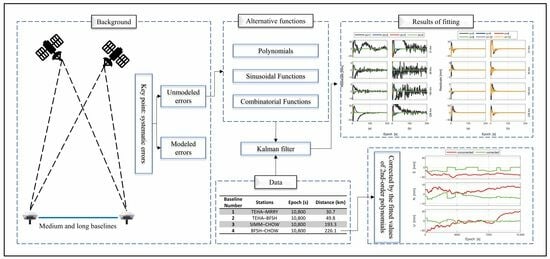
2. Data and Methodology

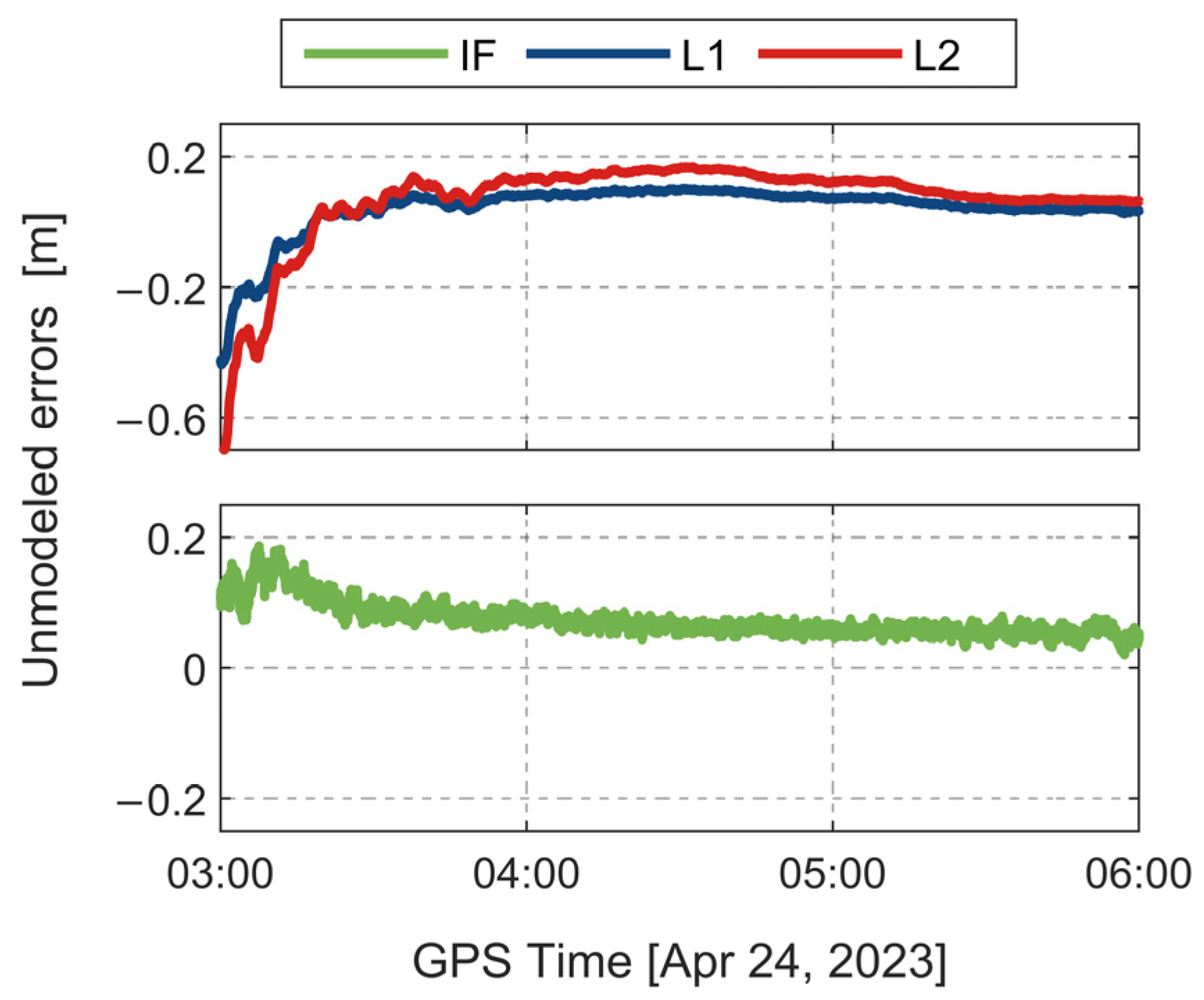
2.1. Unmodeled Error Data

To select a reasonable basic function for a time-varying unmodeled error, unmodeled error data are required. This section describes the source of unmodeled errors and the method used to obtain them.

2.1.1. Baseline Data

The observation files were obtained from the website http://garner.ucsd.edu/pub/highrate/cache/rinex/2023/114/ (accessed on 29 September 2023). The data used in this paper were collected on 24 April 2023 from 0:00:00 to 5:59:59 GPS Time. We used the 3 h data from 3:00:00 to 5:59:59 GPS Time to invert the unmodeled errors, which ensured that the prior-convergence errors were not included in the results. The sampling interval was 1 s. Details of the stations and the baselines used in the inversion process are shown in

Table 1. Details of the stations and baselines.

Baseline Number	Base Station–Rover Station	Observation Type	Receiver Type at the Base Station	Antenna and Radome Types at the Base Station	Epoch (s)	Distance (km)
1	TEHA–MRRY	L1C, L2W	TRIMBLE NETR9	TRM57971.00 NONE	10,800	30.7
2	TEHA–BFSH	L1C, L2W	TRIMBLE NETR9	TRM57971.00 NONE	10,800	49.8
3	SIMM–CHOW	L1C, L2W	TRIMBLE NETR9	TRM57971.00 NONE	10,800	193.3
4	BFSH–CHOW	L1C, L2W	TRIMBLE NETR5	TRM57971.00 NONE	10,800	226.1

.

The stations in Table 1 belong to the UFCORS Center of the NOAA. The coordinates of each station in Table 1 can be obtained from the weekly solution files. The precise ephemeris and other products used in the subsequent experiments were retrieved from the IGS.

2.1.2. Inversion of Unmodeled Errors

We applied the unmodeled error inversion procedure proposed in a previous study [3] to the data of the four baselines in Table 1. The specific inversion procedure consists of four steps: (1) the establishment of carrier-phase double-difference (DD) observation equations, (2) the calculation of the DD distance between receivers and satellites, (3) processing atmospheric delays, and (4) the resolution of integer ambiguity and the calculation of unmodeled errors.

Some research has pointed out that the specific values and characteristics of the unmodeled errors are closely related to the positioning modes [20]. Therefore, in the present contribution, we investigated the unmodeled errors in two widely used differential positioning modes, which are detailed in

Table 2. Positioning settings for three positioning modes.

Categories	Settings
	Estimating Atmospheric Delays	Using IF Combination
Observations	Uncombined L1, L2	$\frac{f_1^2{L}_1-f_2^2{L}_2}{f_1^2-f_2^2}$
Stochastic model	${\sigma }^2=a^2+\frac{b^2}{{\sin }^2(el)}$	${\sigma }^2=a^2+\frac{b^2}{{\sin }^2(el)}$
Cut-off angle	10 degrees	10 degrees
Parameter estimation	Extended Kalman filter	Extended Kalman filter
Satellite orbit	Precise ephemeris	Precise ephemeris
Clock bias	DD	DD
Ionospheric delay	DD + Parameter estimation	DD + IF combination
Tropospheric delay	DD + Parameter estimation	DD + Parameter estimation
Relativistic effect	Model correction	Model correction
Earth Solid Tide	IERS 2010	IERS 2010
Ambiguity resolution	Continuous	Continuous

. Specifically, we addressed the selection of the unmodeled error basic functions in the following differential modes: estimating atmospheric delays and using the ionospheric-free (IF) combination.

In Table 2, the positioning parameters were estimated along with other parameters such as ambiguity. The numerical settings of the parameters to be estimated during the solving process were assumed to be equal to those in the RTKLIB software (version 2.4.3 b34) [26]. The initial values of the positioning parameters were obtained from the single-point positioning (SPP) results, and the initial variance was set to 900 ${\mathrm{m}}^2$. The initial value of the ambiguity parameter was calculated from the pseudorange and phase observations with the initial variance set to 900 ${\mathrm{cycle}}^2$ and the process noise set to ${10}^{-8}$ ${\mathrm{cycle}}^2$. For the ionospheric delay, the initial value was set to ${10}^{-6}$ m, and its initial variance and the variance of the process noise were determined using Equation (1).

$$\begin{array}{l}{\sigma }_{iono}^2={\left(st{d}_{iono}\cdot bl/{10}^4\right)}^2\\ q_{iono}^2={\left(pr{n}_{iono}\cdot bl/{10}^4\right)}^2\cdot \mathsf{\Delta }t\end{array}$$

(1)

where $st{d}_{iono}$ stands for the standard deviation factor of the ionospheric delay parameter and takes a value of 0.03, $pr{n}_{iono}$ stands for the standard deviation factor of the process noise and takes a value of ${10}^{-3}$, $bl$ stands for the approximate length (unit: m) of the baseline, and $\mathsf{\Delta }t$ represents the time interval between the current epoch and the initial epoch. For the tropospheric delay, the initial value was set to 0.15 m, and its initial variance and the variance of process noise were determined using Equation (2).

$$\begin{array}{l}{\sigma }_{trop}^2={\left(st{d}_{trop}\right)}^2\\ q_{trop}^2={\left(pr{n}_{trop}\right)}^2\cdot \mathsf{\Delta }t\end{array}$$

(2)

where $st{d}_{trop}$ stands for the variance factor of the tropospheric delay parameter and takes a value of 0.3, $pr{n}_{trop}$ stands for the variance factor of the process noise and takes a value of ${10}^{-4}$, and $\mathsf{\Delta }t$ stands for the time interval between the current epoch and the initial epoch.

For the above two positioning modes (i.e., estimating atmospheric delays and using the IF combination), the specific form of the carrier equation established in the first step is as follows [3]:

$$\left\{\begin{array}{c}\lambda \cdot \nabla \mathsf{\Delta }\varphi =\nabla \mathsf{\Delta }\rho +\lambda \cdot \nabla \mathsf{\Delta }N+\nabla \mathsf{\Delta }I+\nabla \mathsf{\Delta }T+\lambda \cdot \nabla \mathsf{\Delta }{U}_{EST}\\ {\lambda }_{IF}\cdot \nabla \mathsf{\Delta }{\varphi }_{IF}=\nabla \mathsf{\Delta }\rho +{\lambda }_{IF}\nabla \mathsf{\Delta }{N}_{IF}+\nabla \mathsf{\Delta }T+{\lambda }_{IF}\cdot \nabla \mathsf{\Delta }{U}_{IF}\end{array}\right.$$

(3)

where $\lambda$ and ${\lambda }_{IF}$ stand for the uncombined and combined wavelengths, respectively; $\nabla \mathsf{\Delta }$ denotes the DD operator; $\nabla \mathsf{\Delta }\varphi$ and $\nabla \mathsf{\Delta }{\varphi }_{IF}$ represent the uncombined and combined carrier observations, respectively; $\nabla \mathsf{\Delta }\rho$ is the distance between the receivers and satellites after the DD; $\nabla \mathsf{\Delta }N$ and $\nabla \mathsf{\Delta }{N}_{IF}$ represent the uncombined and combined ambiguity parameters, respectively; $\nabla \mathsf{\Delta }I$ and $\nabla \mathsf{\Delta }T$ stand for the ionospheric delay and tropospheric delay to be estimated, respectively; and $\nabla \mathsf{\Delta }{U}_{EST}$ and $\nabla \mathsf{\Delta }{U}_{IF}$ correspond to the unmodeled errors corresponding the two positioning modes, respectively.

After the positioning models were established, the true DD distance between the receivers and the satellite’s antenna $\nabla \mathsf{\Delta }\rho$ was calculated using the known station coordinates and the satellite coordinates from the final precise ephemeris and the ANTEX file of the IGS. Then, the modeled part of each systematic error and the optimal estimate of ambiguity were calculated following the specific steps in [3]. Finally, the unmodeled error estimates were obtained as follows:

$$\left\{\begin{array}{c}\nabla \mathsf{\Delta }{U}_{EST}=\nabla \mathsf{\Delta }\varphi -\nabla \mathsf{\Delta }\rho /\lambda -\nabla \mathsf{\Delta }N-\nabla \mathsf{\Delta }I/\lambda -\nabla \mathsf{\Delta }T/\lambda \\ \nabla \mathsf{\Delta }{U}_{IF}=\nabla \mathsf{\Delta }{\varphi }_{IF}-\nabla \mathsf{\Delta }\rho /{\lambda }_{IF}-\nabla \mathsf{\Delta }{N}_{IF}-\nabla \mathsf{\Delta }T/{\lambda }_{IF}\end{array}\right.$$

(4)

which indicates that the unmodeled errors vary with different positioning modes.

Following Equation (4), we inverted the unmodeled errors of the four baselines in Table 1 and obtained the corresponding time series. Taking the DD satellite pair composed of G31−G10 in the baseline SIMM-CHOW as an example, the unmodeled errors are shown in Figure 1.

From Figure 1, it can be seen that unmodeled errors range from −0.6 m to 0.2 m, even after 3 h of continuous observation. In addition, the trends of the time series corresponding to the unmodeled errors for the L1 and L2 frequencies are quite similar, indicating that the unmodeled errors are correlated among frequencies. These findings are in line with those of a previous study [3].

2.2. Methodology

After obtaining the unmodeled error data, we needed to determine an optimal basic function to fit it, which is beneficial for making good use of its time correlation in future research. First, three alternative basic functions are introduced in this section. Some significance tests were required, and their statistics are introduced. Furthermore, two indexes are identified for evaluation. Eventually, we designed positioning experiments to demonstrate the usability of the fitted unmodeled errors.

2.2.1. Alternative Basic Functions

From former investigations [3,23], the unmodeled error time series may include some trend terms and periodic terms in which the periodic components are likely to arise from atmospheric delays and multipath effects, as demonstrated by the experiments. Therefore, we described the trend term of the unmodeled errors with a polynomial and described the periodic terms with some sinusoidal functions, as follows:

$$\nabla \mathsf{\Delta }U=a_0+a_{1}t+\cdots +a_m{t}^m={\displaystyle \sum _{i=0}^m{a}_i{t}^i}$$

(5)

$$\nabla \mathsf{\Delta }U=b_1\sin \left(2\pi t{f}_1+{\phi }_1\right)+\cdots +b_n\sin \left(2\pi t{f}_n+{\phi }_n\right)={\displaystyle \sum _{j=1}^n{b}_j\sin \left(2\pi t{f}_j+{\phi }_j\right)}$$

(6)

$$\nabla \mathsf{\Delta }U={\displaystyle \sum _{i=0}^m{a}_i{t}^i}+{\displaystyle \sum _{j=1}^n{b}_j\sin \left(2\pi t{f}_j+{\phi }_j\right)}$$

(7)

where $\nabla \mathsf{\Delta }U$ represents the unmodeled error obtained in the last section and $t$ represents the time interval from the initial epoch; $m$ and $n$ represent the orders of the polynomials and the number of sinusoidal functions, respectively; and $f_j(j=1,\cdots ,n)$ represents the frequency of each sinusoidal function, which is determined by the significant frequency components of the Fourier transform results from the previous study [3]. The range of the values taken by $f_j(j=1,\cdots ,n)$ is mainly concentrated in $4\times {10}^{-4}\sim 5\times {10}^{-3}$ Hz; $a_i(i=1,\cdots ,m)$ and $b_j(j=1,\cdots ,n)$ represent the coefficients of the polynomials and the amplitudes of the sinusoidal functions, respectively, which are estimated via the Kalman filter; and ${\phi }_j(j=1,\cdots ,n)$ is the initial phase to be estimated.

Assume that satellites $s_1$ and $s_2$ are observed simultaneously by receivers $r_1$ and $r_2$ at epoch $t$. Taking the basic function shown in Equation (7) as an example, the unmodeled error model corresponding to L1 can be listed at this epoch as follows:

$$\nabla \mathsf{\Delta }{U}_{r_1{r}_2,L1}^{s_1{s}_2}={\displaystyle \sum _{i=0}^m{a}_i{}_{r_1{r}_2,L1}^{s_1{s}_2}{t}^i}+{\displaystyle \sum _{j=1}^n{b}_j{}_{r_1{r}_2,L1}^{s_1{s}_2}\sin \left(2\pi t{f}_j+{\phi }_j\right)}=HX$$

(8)

where

$$\begin{array}{l}H=\left[\begin{array}{ccccccccc}1& \cdots & t^m& \sin (2\pi f_1)& \cos (2\pi f_1)& \cdots & \cdots & \sin (2\pi f_n)& \cos (2\pi f_n)\end{array}\right]\\ X={\left[\begin{array}{ccccccccc}{a}_0& \cdots & a_m& b_1\cos {\phi }_1& b_1\sin {\phi }_1& \cdots & \cdots & b_n\cos {\phi }_n& b_n\sin {\phi }_n\end{array}\right]}^T\end{array}$$

(9)

Meanwhile, the state equation is given as follows:

$$X_t=X_{t-1}+{\eta }_t$$

(10)

where ${\eta }_t\sim N(0,Q_t)$ stands for the process noise of the state vector and $Q_t={10}^{-3}\cdot I_{(m+n)\times (m+n)}$.

Then, we can estimate the parameters using a Kalman filter. The unknown parameters in the other two basic functions are estimated in a similar way and, for brevity, they are not introduced again.

2.2.2. Model Testing and Evaluation

Once the parameters are solved, the models need to be tested. First, the models must be tested for their overall significance, and the original and alternative hypotheses are as follows:

$$\begin{array}{l}{H}_0:a_0=a_1=\cdots =a_m=b_1=\cdots =b_n=0\\ H_1:a_i(i=0,1,\cdots ,m{) \mathrm{and} \mathrm{b}}_i(i=1,\cdots ,n) \mathrm{are} \mathrm{not} \mathrm{all} \mathrm{equal} \mathrm{to} 0\end{array}$$

(11)

where $H_0$ represents the original hypothesis and $H_1$ represents the alternative hypothesis. The corresponding statistic is calculated as follows:

$$f=\frac{{\displaystyle \sum {({\widehat{y}}_i-\overline{y})}^2}/k}{{\displaystyle \sum {(y_i-{\widehat{y}}_i)}^2}/(n-k-1)}$$

(12)

where $y_i$ represents the value of the unmodeled error obtained via the inversion; ${\widehat{y}}_i$ is the estimate of the unmodeled error calculated using the model; $\overline{y}$ is the mean of $y_i$; and $k$ and $n$ represent the number of variables and samples, respectively. The statistic $f$ follows a distribution of $F(k,n-k-1)$ where $k$ and $n-k-1$ are the degrees of freedom of the Fisher–Snedecor distribution [27].

After taking the significance level $\alpha =0.05$, $F(k,n-k-1)$ and $f$ can be compared. If $f<F_{\alpha }(k,n-k-1)$, the original hypothesis is accepted, indicating that the model is not significant; otherwise, the original hypothesis is rejected, indicating that the model is significant.

After the model is tested to be significant, the second step requires a significance test for each estimated parameter. For each parameter ${\beta }_i$, we can calculate a statistic $t$ that follows the distribution of $t(n-k-1)$ where $n-k-1$ represents the degree of freedom for Student’s t-distribution [27]. After taking the significance level $\alpha =0.05$, the critical value $t_{\alpha /2}(n-k-1)$ can be checked. If $\left|t\right|<t_{\alpha /2}(n-k-1)$, it means that the parameter ${\beta }_i$ is not significantly different from zero. On the contrary, it means that the parameter ${\beta }_i$ is significantly not equal to zero. If a parameter is not significant, the corresponding variable should be removed, and the model should be rebuilt.

After the model test, we chose two indexes, the R-square and Root Mean Square Error (RMSE), to evaluate the corresponding model. The closer the RMSE is to zero, the higher the overall accuracy of this alternative basic function. The value of the R-square ranges from 0 to 1, and the closer it is to 1, the better the model fits.

2.2.3. Positioning Verification

To verify the applicability of the fitted unmodeled errors, we carried out positioning experiments. The main idea was to perform the regular positioning process after correcting the DD observations using the fitted unmodeled errors. The results of this positioning are then compared with the uncorrected positioning results.

Taking the mode of estimating atmospheric delays in Equation (3) as an example, the uncorrected observation equation is

$$\lambda \cdot \nabla \mathsf{\Delta }\varphi =\nabla \mathsf{\Delta }\rho +\lambda \cdot \nabla \mathsf{\Delta }N+\nabla \mathsf{\Delta }I+\nabla \mathsf{\Delta }T+\epsilon$$

(13)

where $\lambda$ stands for the wavelength; $\nabla \mathsf{\Delta }$ denotes the DD operator; $\nabla \mathsf{\Delta }\varphi$ represents the uncorrected carrier observation; $\nabla \mathsf{\Delta }\rho$ is the distance between the receivers and satellites after the DD; $\nabla \mathsf{\Delta }N$ represents the ambiguity parameter; $\nabla \mathsf{\Delta }I$ and $\nabla \mathsf{\Delta }T$ stand for the ionospheric delay and tropospheric delay to be estimated, respectively; and $\epsilon$ corresponds to the observation noise.

The observation equation corrected with the fitted unmodeled errors is

$$\lambda \cdot \left(\nabla \mathsf{\Delta }\varphi -\nabla \mathsf{\Delta }\widehat{U}\right)=\nabla \mathsf{\Delta }\rho +\lambda \cdot \nabla \mathsf{\Delta }N+\nabla \mathsf{\Delta }I+\nabla \mathsf{\Delta }T+\epsilon$$

(14)

where $\nabla \mathsf{\Delta }\widehat{U}$ stands for the estimate of the unmodeled errors from the model.

The above two types of observation equations are solved for positioning separately to obtain the corresponding positioning results. Finally, the deviations between these two kinds of positioning results and the true values are compared separately to verify whether the fitted unmodeled errors are feasible.

3. Results

After preparing the unmodeled error data and determining the alternative basic functions, we conducted modeling experiments for the unmodeled errors under differential positionings: estimating atmospheric delays and using the IF combination in Table 2. First, we conducted the experiments using polynomials and determined the value of $m$ in Equation (5). Second, experiments were carried out using the sinusoidal functions, and the value of $n$ in Equation (6) was analyzed based on the experimental results. Then, combinatorial models were analyzed based on the values of $m$ and $n$. After fitting the unmodeled errors, the positioning experiments were conducted to verify the applicability of the fitted unmodeled errors.

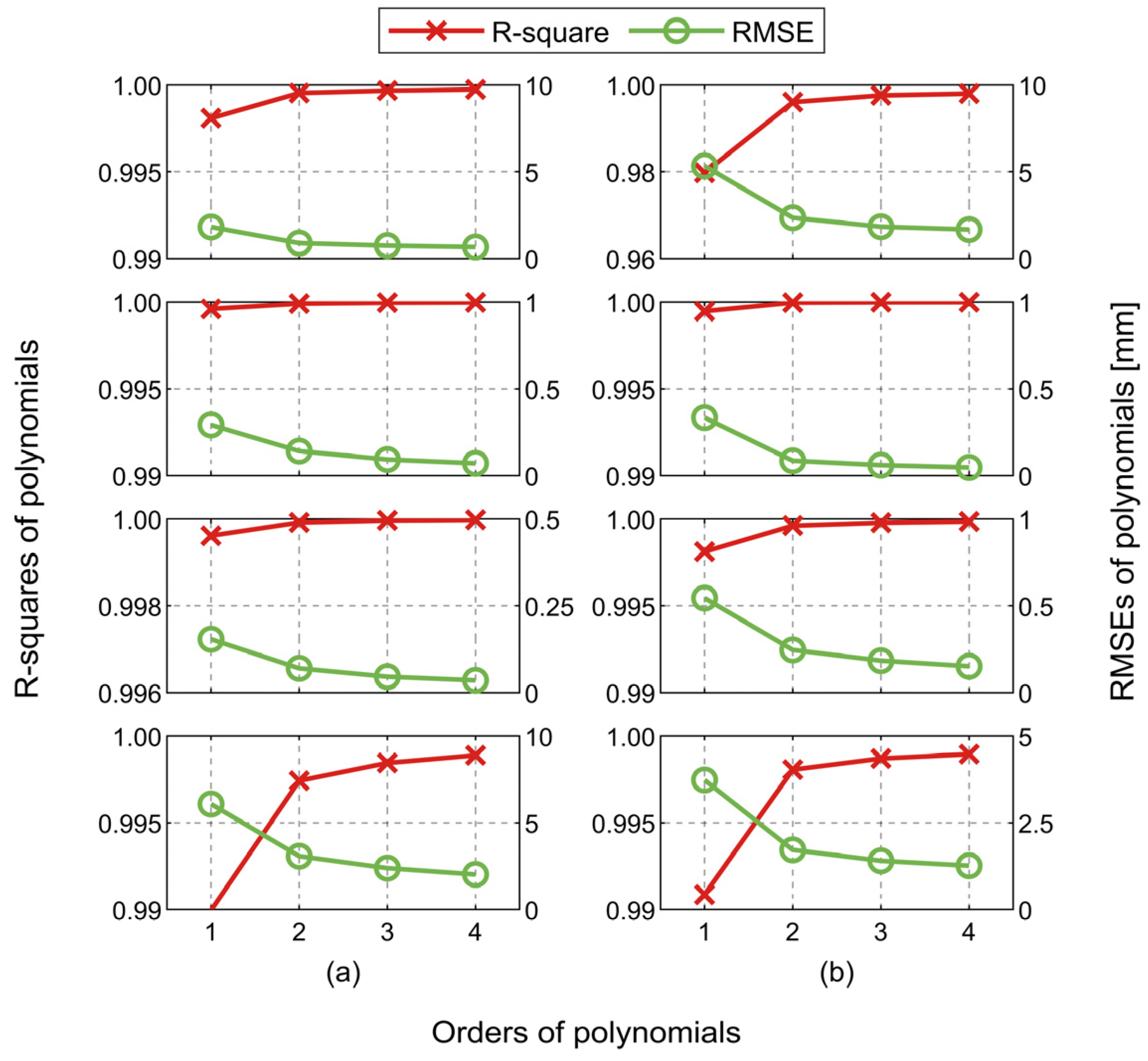
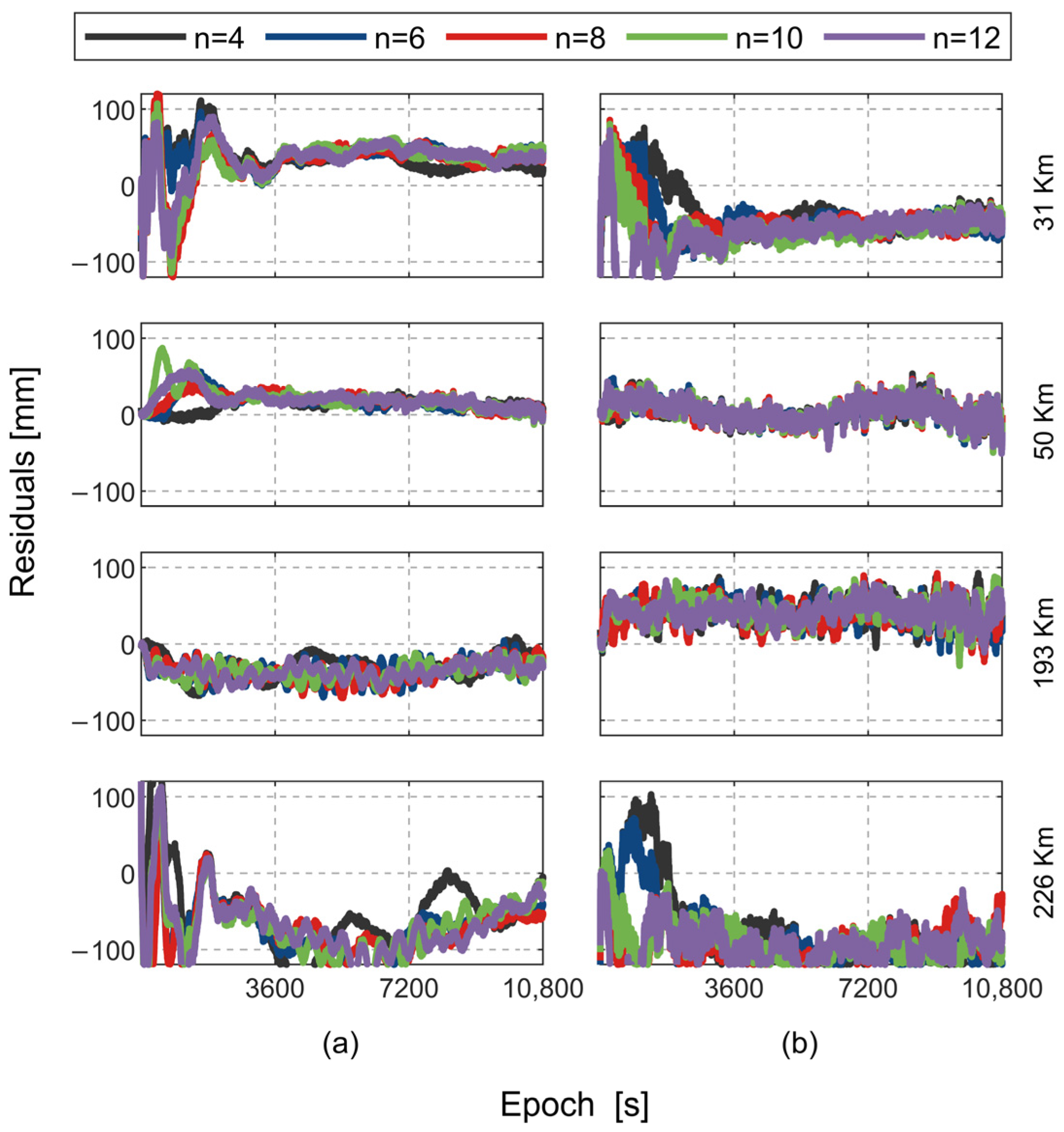
3.1. Fitting Experiments

3.1.1. Polynomials

We fitted the unmodeled errors in differential positionings with polynomials of different orders, as shown in Equation (5). In the experiments in this section, we fitted the unmodeled errors with first-, second-, third-, and fourth-order polynomials, respectively. Taking the unmodeled error data obtained via inversion as the reference, we obtained the residuals of different polynomials. Using the $f_1$ frequency of the DD satellite pairs comprising G31−G01 in baseline No. 1, G31−G10 in baseline No. 3, and G31−G21 in baselines No. 2 and No. 4 as examples, the corresponding residuals are shown in Figure 2. In Figure 2, $m$ refers to the order of the polynomial.

As can be seen from Figure 2, the residuals of polynomials of different orders, as shown in Equation (5), appear to decrease as the number of epochs increases. The second- and higher-order polynomials reach good fitting earlier than the first polynomial. After the 100th epoch, the residuals of the second- and higher-order polynomials are basically less than 1 mm. The differences between these polynomials are mainly within the initial 100 epochs. Specifically, the higher the order of the polynomial, the faster the absolute values of residuals decrease. As expected, the residuals of a polynomial improve as its order increases. In particular, the improvement in residuals is significant for the second-order polynomial compared to the first-order polynomial. In a situation in which the order of the polynomial is greater than two, this improvement is not as significant as from a first-order polynomial to a second-order polynomial. To analyze the effect of order on the polynomial residuals in more detail, we counted a specific epoch in which the residuals of all its subsequent epochs are less than 0.003 m, and this convergence time is depicted in

Table 3. The convergence time of residuals in Figure 2.

Positioning Mode	Baseline Number	Convergence Time (s)
		$\mathit{m}=1$	$\mathit{m}=2$	$\mathit{m}=3$	$\mathit{m}=4$
Estimating atmospheric delays	1	319	25	9	5
	2	68	11	5	1
	3	12	3	3	3
	4	146	30	11	6
Using the IF combination	1	720	39	14	8
	2	243	4	1	1
	3	223	12	6	1
	4	597	35	11	6

. The reason for choosing 0.003 m as the threshold was that the random error of the carrier observations was generally around 0.003 m.

From Table 3, we can conclude that in differential positioning, the higher the order, the faster the residuals converge. It can also be found that the improvement from the first order to second order is the most significant in Table 3. We further calculated the R-squares and RMSEs for each polynomial in Figure 2, as shown in Figure 3.

As can be seen from Figure 3, basically, the R-square of each polynomial is above 0.99, indicating that each polynomial has good fitting. Similar to the residuals, the improvement in the R-square value is also significant when the order is increased from 1 to 2. In terms of the RMSE, the RMSEs of the second-, third-, and fourth-order polynomials are basically less than 2 mm. This illustrates that these three polynomials have high levels of modeling accuracy in general. As for the first-order polynomial, some of its RMSEs are close to or even exceed 5 mm, suggesting that the first-order polynomial is not as accurate as the higher-order polynomials. Therefore, in terms of residuals, convergence time, and overall accuracy, the second- and higher-order polynomials perform better than the first-order polynomials. In addition, the computational cost of these polynomials deserves to be considered, so the processing time of these polynomials was investigated. The time taken to fit the unmodeled errors of one satellite pair for each polynomial was calculated and is shown in

Table 4. Processing time to fit the unmodeled errors of one satellite pair for each polynomial.

Positioning Mode	Processing Time (s)
	$\mathit{m}=1$	$\mathit{m}=2$	$\mathit{m}=3$	$\mathit{m}=4$
Estimating atmospheric delays	0.467	0.592	0.739	0.875
Using the IF combination	0.430	0.586	0.729	0.855

. The time in Table 4 is the average time per fit, calculated after 50 repetitions using a particular polynomial. It should be noted that the experiments were conducted on a computer equipped with an Intel i5-9400 CPU and 32 GB of RAM.

As shown in Table 4, a higher order leads to a longer time required for the fit. For the sake of balancing the effectiveness and computational cost of the fit, we conclude that the second order is the optimal choice when fitting the unmodeled errors with polynomials.

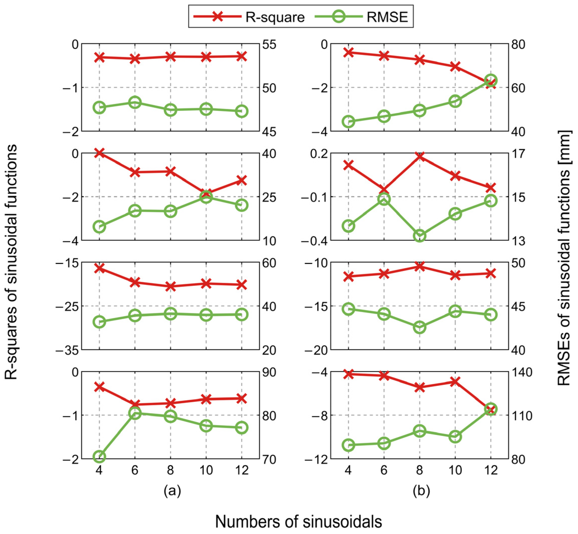
3.1.2. Sinusoidal Functions

In this section, some sinusoidal functions are used to fit the unmodeled errors. The number of the sinusoidal functions $n$ shown in Equation (6) is taken as 4, 6, 8, 10, and 12. Taking the unmodeled error data obtained via inversion as the reference, we can obtain the residuals of different sinusoidal functions. Using the $f_1$ frequency of the DD satellite pairs comprising G31−G01 in baseline No. 1, G31−G10 in baseline No. 3, and G31−G21 in baselines No. 2 and No. 4 as examples, the residuals are shown in Figure 4. In Figure 4, $n$ refers to the number of sinusoidal functions.

As we can see from Figure 4, all the sinusoidal functions exhibit large residuals, regardless of n. When estimating the atmospheric delays or using the IF combination, the residuals of the sinusoidal functions are close to ±0.1 m at the maximum. These results suggest that a trend term may be more prevalent than some periodic terms in the unmodeled errors in medium and long baselines. It is the presence of the trend term that makes it difficult to accurately fit the unmodeled errors with sinusoidal functions alone. As shown in Figure 4, the residuals of these sinusoidal functions do not show convergence, so there is no need to account for the convergence time. As for the accuracy, we calculated R-square and RMSE values for all the sinusoidal functions in Figure 4, as shown in Figure 5.

In Figure 5, most of the sinusoidal functions have negative R-square values. As for the RMSE, the RMSE values of basically all of the sinusoidal functions are in the range of 20 mm to 80 mm, which is from ten to tens of times higher than the RMSEs of the polynomials in the previous section. These phenomena also indicate that it is difficult to accurately fit the unmodeled errors in medium and long baselines when using only sinusoidal functions. Therefore, in the two positioning modes in Table 2, we do not recommend using only the sinusoidal functions to fit the unmodeled errors in baselines above 30 km.

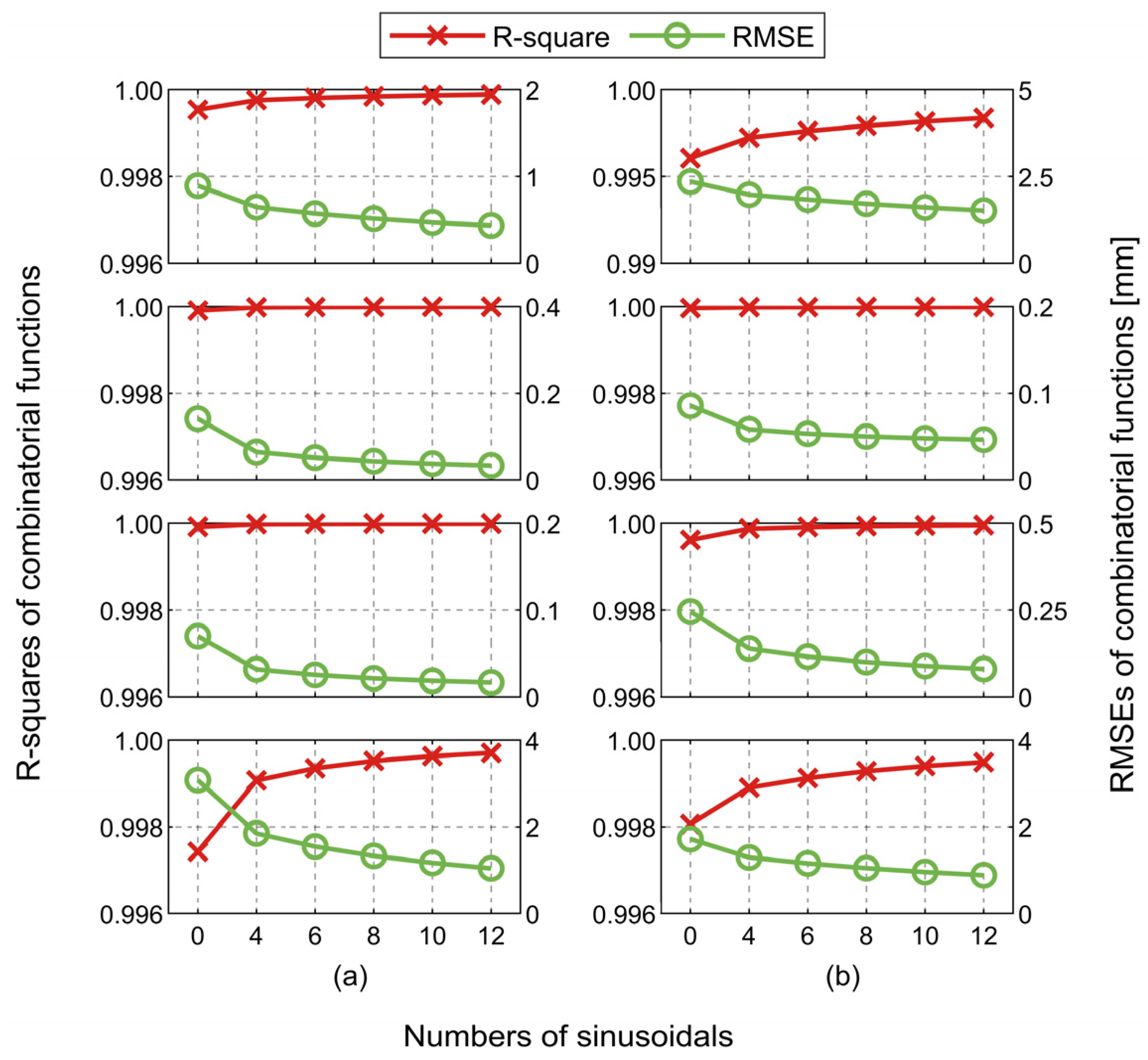
3.1.3. Combinatorial Functions

Although the fit did not perform effectively when using the sinusoidal functions alone, the unmodeled errors in the medium and long baselines do exhibit some periodicity. We therefore investigate whether using a combinatorial function of polynomial and sinusoidal functions yields better results than one or the other alone.

This section analyzes the performance of a combinatorial function, which is in the form of Equation (7), in fitting the unmodeled errors in medium and long baselines. According to the experimental results in the previous two sections, the second-order polynomial is the most appropriate choice when fitting unmodeled errors using polynomials alone. Therefore, in this section, we set the polynomial order in the combinatorial function as 2, that is, the value of $m$ in Equation (7) was determined to be 2. On the basis of this second-order polynomial, we combined it with 4, 6, 8, 10, and 12 sinusoidal functions, respectively, and investigated the fitting performances of these combinatorial functions. Taking the unmodeled error data obtained through inversion as the reference, we also obtained the residuals of different combinatorial functions. Using the $f_1$ frequency of the DD satellite pairs comprising G31−G01 in baseline No. 1, G31−G10 in baseline No. 3, and G31−G21 in baselines No. 2 and No. 4 as examples, the residuals are shown in Figure 6. In Figure 6, $m$ and $n$ refer to the order of the polynomial and the number of sinusoidal functions.

In Figure 6, the black curves represent the residuals of the second-order polynomial, and the other colors represent the combinatorial functions composed of the second-order polynomial and different numbers of sinusoidal functions. From Figure 6, we can see that after the 40th epoch, the black curves basically overlap with the other curves, indicating that after filtering for a period of time, the combinatorial function does not differ significantly from the second-order polynomial. In addition, before the 40th epoch, the performance of the combinatorial function in terms of residuals is slightly improved compared to the second-order polynomial. At the same epoch, the combinatorial functions seem to have smaller residuals than the second-order polynomial. Accordingly, we conjecture that the residuals of the combinatorial functions may converge faster than the second-order polynomial.

To verify the above conjecture, we measured the convergence times of the residuals of the second-order polynomial and the combinatorial functions in Figure 6, as shown in

Table 5. Convergence times of residuals in Figure 6.

Positioning Mode	Baseline Number	Convergence Time (s)
		$\mathit{m}=2, \mathit{n}=0$	$\mathit{m}=2, \mathit{n}=4$	$\mathit{m}=2, \mathit{n}=6$	$\mathit{m}=2, \mathit{n}=8$	$\mathit{m}=2, \mathit{n}=10$	$\mathit{m}=2, \mathit{n}=12$
Estimating atmospheric delays	1	25	21	19	18	18	18
	2	11	7	7	7	7	7
	3	3	2	2	2	2	2
	4	30	25	23	23	23	20
uUsing IF combination	1	39	39	35	35	35	35
	2	4	1	1	1	1	1
	3	12	8	8	8	8	8
	4	35	31	26	26	26	26

. It should be noted that the definition of the convergence time in Table 5 is the same as the definition in Table 3.

As presented in Table 5, the combinatorial function has a shorter convergence time for the residuals compared to the second-order polynomial when estimating the atmospheric delays and using the IF combination. However, the convergence time of the combinatorial function is only three or four seconds shorter than that of the second-order polynomial. This indicates that the improvement of the combinatorial function over the second-order polynomial is not significant.

To compare the overall accuracy, we compared the R-square and RMSE values of the combinatorial functions and the second-order polynomial; see Figure 7.

In Figure 7, all the R-square values are above 0.99, and all the RMSEs are basically below 2 mm, which confirms that both the second-order polynomial and the combinatorial functions in Figure 7 are outstanding in terms of their accuracy. After adding the sinusoidal functions, the differences of the residuals between the combinatorial functions and the polynomials are quite insignificant. In terms of R-square values, the improvements of the combinatorial functions are roughly 0.001, and in terms of RMSEs, the improvements of the combinatorial functions are basically less than 1 mm. These results indicate that adding the sinusoidal functions does not provide a significant improvement in terms of the overall accuracy. This may imply that the trend term accounts for a more important component of the unmodeled errors in medium and long baselines. This may also be the reason for which a good fit can be achieved with polynomials alone.

Finally, we analyzed the performance of the combinatorial functions in terms of processing time. We calculated the average time used to fit the unmodeled errors for one satellite pair for each combinatorial function, as shown in

Table 6. Processing time to fit the unmodeled errors of one satellite pair for second-order polynomial and combinatorial functions.

Positioning Mode	Processing Time (s)
	$\mathit{m}=2, \mathit{n}=0$	$\mathit{m}=2, \mathit{n}=4$	$\mathit{m}=2, \mathit{n}=6$	$\mathit{m}=2, \mathit{n}=8$	$\mathit{m}=2, \mathit{n}=10$	$\mathit{m}=2, \mathit{n}=12$
Estimating atmospheric delays	0.592	1.306	1.595	1.909	2.068	2.531
Using IF combination	0.586	1.284	1.598	1.905	2.214	2.533

. The time in Table 6 has the same definition as that in Table 4.

Table 6 shows that the more sinusoidal functions there are in a combinatorial function, the longer the time required for the fit is. The time required for the combinatorial function is about two to five times longer than that of the second-order polynomial. Therefore, we recommend the second-order polynomial as the basic function for unmodeled errors due to its processing time and overall accuracy because the combinatorial function takes several times the time of the second-order polynomial but only obtains a marginal improvement. In terms of the convergence time of the residuals, when estimating atmospheric delays or using the IF combinations, the second-order polynomial is still a worthwhile basic function to use.

3.2. Positioning Experiments

Following the relevant methodology in Section 2.2.3, we performed positioning experiments using the No. 4 baseline in Table 1 as an example. The positioning experiments used two modes: estimating atmospheric delays and ionospheric-free combination. Under the different positioning modes, we first utilized the uncorrected observations for the positioning. Second, we brought the unmodeled errors obtained from the best performing second-order polynomial in the fitting experiments into Equation (14) and performed the positioning again. The deviations of the positioning results are shown in Figure 8 and Figure 9.

In Figure 8 and Figure 9, the red and green curves represent the positioning deviations of the uncorrected observations and the corrected observations, respectively. It can be seen that the positioning deviation of the corrected observations is significantly improved over the uncorrected observations. It should be noted that the observation data used in this section are also from the last 10,800 epochs of the data described in Section 2.1.1. Therefore, the convergence process is unobservable in Figure 8 and Figure 9. For most epochs, the deviations of the corrected results are closer to zero than the uncorrected results.

We also counted the RMSEs of the positioning results for the uncorrected and the corrected observations, as shown in

Table 7. RMSEs of the positioning results for the uncorrected and the corrected observations.

Positioning Mode	Directions	RMSEs of Uncorrected Positioning (m)	RMSEs of Corrected Positioning (m)	Improvement (%)
estimating atmospheric delays	E	0.0224	0.0080	64.29
	N	0.0051	0.0031	39.22
	U	0.0165	0.0033	80.00
using IF combination	E	0.0115	0.0109	5.22
	N	0.0088	0.0053	39.77
	U	0.0184	0.0066	64.13

.

As it can be seen in Table 7, the observations corrected for the unmodeled errors from the second-order polynomial provide a remarkably significant improvement in terms of the positioning results. When estimating atmospheric delays, the improvement effects in the three directions are 64.29%, 39.22%, and 80.00%, respectively. When using the IF combination, the improvement effects in the three directions are 5.22%, 39.77%, and 64.13%, respectively. These improvements in the positioning results indicate that the fitted values incorporated into Equation (14) are able to reflect, at least in part, the reality of the unmodeled errors in the observation equations. Also, these experiment results demonstrate the usability of fitting the unmodeled errors for positioning using the second-order polynomial.

4. Discussion

Previous studies [3,23] indicated that the unmodeled errors contain periodic components. The frequency range of these periodic components is mainly $4\times {10}^{-4}\sim 5\times {10}^{-3}$ Hz, corresponding to a time range of about 200~2500 s. In this paper, when fitting the unmodeled errors with the sinusoidal or combinatorial functions, the chosen frequency ranges were also concentrated in the $4\times {10}^{-4}\sim 5\times {10}^{-3}$ Hz range. However, from Figure 4, it can be found that a good result cannot be obtained when a sinusoidal function alone is used to fit the unmodeled errors. Meanwhile, from Figure 6 and Figure 7 and Table 5, it can be found that the addition of sinusoidal functions improves the fitting effect but quite minimally when using a combinatorial function. From these experimental results, we can conclude that the periodic components of the unmodeled errors represent a minor proportion and that most of the components behave as trend term signals.

Previous studies also concluded that atmospheric delays are the main component of GNSS unmodeled errors. Meanwhile, noting that the unmodeled error time series used in this paper lasted 3 h, the experiments also imply that the atmospheric delays are relatively stable within 3 h. The periodic components ($4\times {10}^{-4}\sim 5\times {10}^{-3}$ Hz) may be mainly attributed to the multipath effect and some uncorrected receiver bias and are not the main proportion of unmodeled errors. This explains why the unmodeled errors can be fitted well using polynomial functions alone and limits the conclusion of this paper to the short-term modeling of unmodeled errors. This application is relevant to real-time navigation.

Another reason for the minor proportion of the periodic components in the unmodeled error may be related to the estimation of the unmodeled errors. The main source of the unmodeled errors obtained from the inversion in this paper was the component in the positioning and the ambiguity parameters. During the solving process, it is possible that the errors absorbed by the static positioning and the ambiguity parameter were mainly non-periodic components. Most of the periodic components were absorbed by other parameters. These parameters cannot be considered in the inversion method of this paper because it is difficult to obtain their true values.

In the positioning experiments, there is a significant improvement in the positioning results corrected by the fitted unmodeled errors. This indicates that the fitted, unmodeled errors were consistent with the actual unmodeled errors in the observation equations. There was still some deviation between the improved positioning results and the true values because the original modeled errors were still present in the observations. When positioning with observations corrected for unmodeled errors, these originally modeled errors affected the parameter estimates in the current epoch. However, these modeled errors were smaller compared to the errors in the uncorrected equations, explaining the larger improvement over the original positioning results, although the corrected results still deviated somewhat from the true values.

5. Conclusions

The present study addressed some basic functions to account for unmodeled errors in medium and long GNNSS baselines in two differential positioning modes: estimating atmospheric delays and using the IF combination. We used four baselines ranging from 30 to 220 km to invert an unmodeled error time series to provide a reference residual. We then selected three alternative basic functions including polynomials, sinusoidal functions, and combinatorial functions, and methods for their solution, testing, and evaluation methods were introduced. At last, fitting experiments and positioning experiments were conducted to analyze and compare these three basic functions.

The experimental results can be summarized as follows. (1) When fitting unmodeled errors with polynomials in a long baseline, the second-order polynomial is the optimal choice. Compared with the first-order polynomial, the second-order polynomial has higher accuracy and a faster convergence of residuals. Compared with higher-order polynomials, the second-order polynomial is more efficient in the case of ensuring comparable accuracy. (2) It is difficult to achieve high-accuracy results by fitting the unmodeled errors with sinusoidal functions only. (3) The combinatorial functions have basically no advantage compared with the second-order polynomial in short-term cases. When estimating atmospheric delays or using the IF combination, the combinatorial functions are essentially comparable to the second-order polynomial in terms of residual convergence time and overall accuracy but takes several times longer than the second-order polynomial. (4) After the observations have been corrected by the fitted unmodeled errors from the second-order polynomial, a remarkably significant improvement appears in terms of the positioning results, which demonstrates the usability of fitting the unmodeled errors for positioning using the second-order polynomial.

Based on the above experimental findings, we suggest that a second-order polynomial can be used as the basic function for a short-term time-varying model of unmodeled errors in medium and long baselines. Further work needs to be carried out in order to add the basic functions into the positioning process of long baselines to estimate model parameters in real time.

References

1. Shen, N.; Chen, L.; Wang, L.; Chen, R. GNSS Site unmodeled error prediction based on machine learning. GPS Solut. 2023, 27, 77. [Google Scholar] [CrossRef]
2. Zhang, Z.; Li, B.; Shen, Y. Comparison and analysis of unmodelled errors in GPS and BeiDou signals. Geod. Geodyn. 2017, 8, 41–48. [Google Scholar] [CrossRef]
3. Wang, J.; Yu, X.; Guo, S. Inversion and characteristics of unmodeled errors in GNSS relative positioning. Measurement 2022, 195, 111151. [Google Scholar] [CrossRef]
4. Klobuchar, J. Ionospheric time-delay algorithms for single-frequency GPS users. IEEE Trans. Aerosp. Electron. Syst. 1987, AES-23, 325–331. [Google Scholar] [CrossRef]
5. Giovanni, G.D.; Radicella, S.M. An analytical model of the electron density profile in the ionosphere. Adv. Space Res. 1990, 10, 27–30. [Google Scholar] [CrossRef]
6. Yuan, Y.; Wang, N.; Li, Z.; Huo, X. The BeiDou global broadcast ionospheric delay correction model (BDGIM) and its preliminary performance evaluation results. Navigation 2019, 66, 55–69. [Google Scholar] [CrossRef]
7. Li, X.; Li, X.; Liu, G.; Feng, G.; Yuan, Y.; Zhang, K.; Ren, X. Triple-frequency PPP ambiguity resolution with multi-constellation GNSS: BDS and Galileo. J. Geod. 2019, 93, 1105–1122. [Google Scholar] [CrossRef]
8. Hopfield, H. Two-quartic tropospheric refractivity profile for correcting satellite data. J. Geophys. Res. 1969, 74, 4487–4499. [Google Scholar] [CrossRef]
9. Saastamoinen, J. Contributions to the theory of atmospheric refraction. Bull. Geod. 1973, 107, 13–34. [Google Scholar] [CrossRef]
10. Lagler, K.; Schindelegger, M.; Böhm, J.; Krásná, H.; Nilsson, T. GPT2: Empirical slant delay model for radio space geodetic techniques. Geophys. Res. Lett. 2013, 40, 1069–1073. [Google Scholar] [CrossRef]
11. Schüler, T. The TropGrid2 standard tropospheric correction model. GPS Solut. 2014, 18, 123–131. [Google Scholar] [CrossRef]
12. Yao, Y.; Zhang, B.; Xu, C.; He, C.; Yu, C.; Yan, F. A global empirical model for estimating zenith tropospheric delay. Sci. China Earth Sci. 2016, 59, 118–128. [Google Scholar] [CrossRef]
13. Marini, J.W. Correction of Satellite Tracking Data for an Arbitrary Tropospheric Profile. Radio Sci. 1972, 7, 223–231. [Google Scholar] [CrossRef]
14. Böhm, J.; Schuh, H. Vienna mapping functions in VLBI analyses. Geophys. Res. Lett. 2004, 31, L01603. [Google Scholar] [CrossRef]
15. Yuan, L.; Huang, D.; Ding, X.; Xiong, Y.; Zhong, P.; Li, C. On the influence signal multipath effects in GPS carrier phase surveying. Acta Geod. Cartogr. Sin. 2004, 33, 210–215. [Google Scholar] [CrossRef]
16. Zhong, P.; Ding, X.; Zheng, D.; Chen, W. An adaptive wavelet transform based on crossvalidation and its application to mitigate GPS multipath effects. Acta Geod. Cartogr. Sin. 2007, 36, 279–285. [Google Scholar] [CrossRef]
17. Zhong, P.; Ding, X.; Yuan, L.; Xu, Y.; Kwok, K.; Chen, Y. Sidereal filtering based on single differences for mitigating GPS multipath effects on short baselines. J. Geod. 2010, 84, 145–158. [Google Scholar] [CrossRef]
18. Dong, D.; Wang, M.; Chen, W.; Zeng, Z.; Song, L.; Zhang, Q.; Cai, M.; Cheng, Y.; Lv, J. Mitigation of multipath effect in GNSS short baseline positioning by the multipath hemispherical map. J. Geod. 2016, 90, 255–262. [Google Scholar] [CrossRef]
19. Hernández-Pajares, M.; Aragón-Ángel, À.; Defraigne, P.; Bergeot, N.; Prieto-Cerdeira, R.; García-Rigo, A. Distribution and mitigation of higher-order ionospheric effects on precise GNSS processing. J. Geophys. Res. Solid Earth 2014, 119, 3823–3837. [Google Scholar] [CrossRef]
20. Zhang, Z.; Li, B. Unmodeled error mitigation for single-frequency multi-gnss precise positioning based on multi-epoch partial parameterization. Measur. Sci. Technol. 2020, 31, 025008. [Google Scholar] [CrossRef]
21. Zhang, Z.; Li, Y.; He, X.; Hsu, L. Resilient GNSS real-time kinematic precise positioning with inequality and equality constraints. GPS Solut. 2023, 27, 116. [Google Scholar] [CrossRef]
22. Li, B.; Zhang, Z.; Shen, Y.; Yang, L. A procedure for the significance testing of unmodeled errors in GNSS observations. J. Geodesy 2018, 92, 1171–1186. [Google Scholar] [CrossRef]
23. Zhang, Z.; Li, B.; Shen, Y.; Gao, Y.; Wang, M. Site-specific unmodeled error mitigation for GNSS positioning in urban environments using a real-time adaptive weighting model. Remote Sens. 2018, 10, 1157. [Google Scholar] [CrossRef]
24. Yuan, H.; Zhang, Z.; He, X.; Li, G.; Wang, S. Stochastic model assessment of low-cost devices considering the impacts of multipath effects and atmospheric delays. Measurement 2022, 188, 110619. [Google Scholar] [CrossRef]
25. Zhang, Z.; Yuan, H.; He, X.; Chen, B.; Zhang, Z. Unmodeled-error-corrected stochastic assessment for a standalone GNSS receiver regardless of the number of tracked frequencies. Measurement 2023, 206, 112265. [Google Scholar] [CrossRef]
26. Takasu, T. RTKLIB: Open Source Program Package for RTK-GPS, FOSS4G 2009, Tokyo, Japan, 2 November 2009. Available online: https://gpspp.sakura.ne.jp/rtklib/rtklib.htm (accessed on 17 January 2023).
27. Hawkes, A.G. Statistical Models in Applied Science; Bury, K.V., Ed.; Wiley: London, UK, 1975; ISBN 0-471-12590-3. [Google Scholar] [CrossRef]
Figure 1. Unmodeled errors of the G31−G10 satellite pair in No. 3 baseline in differential positioning modes.
Remotesensing 15 05022 g001
Figure 2. Residuals of different polynomials for DD satellite pairs of baselines No. 1~4 in differential positionings. Columns (a,b) display “estimating atmospheric delays” and “using IF combination”, respectively.
Remotesensing 15 05022 g002
Figure 3. R-squares and RMSEs of different polynomials for DD satellite pairs of baselines No. 1~4 in differential positionings. Columns (a,b) display “estimating atmospheric delays” and “using IF combination”, respectively.
Remotesensing 15 05022 g003
Figure 4. Residuals of sinusoidal functions for the DD satellite pairs of baselines No. 1~4 in differential positionings. Columns (a,b) display “estimating atmospheric delays” and “using IF combination”, respectively.
Remotesensing 15 05022 g004
Figure 5. R-square and RMSE values of the sinusoidal functions for DD satellite pairs of baselines No. 1~4 in differential positionings. Columns (a,b) display “estimating atmospheric delays” and “using IF combination”, respectively.
Remotesensing 15 05022 g005
Figure 6. Residuals of combinatorial functions for DD satellite pairs of baselines No. 1~4 in differential positionings. Columns (a,b) display “estimating atmospheric delays” and “using IF combination”, respectively.
Remotesensing 15 05022 g006
Figure 7. R-square and RMSE values of the combinatorial functions for the DD satellite pairs of baselines No. 1~4 in differential positionings. Columns (a,b) display “estimating atmospheric delays” and “using IF combination”, respectively.
Remotesensing 15 05022 g007
Figure 8. Positioning deviations for uncorrected observations and corrected observations in the mode of estimating atmospheric delays.
Remotesensing 15 05022 g008
Figure 9. Positioning deviations for uncorrected observations and corrected observations in the mode of IF combination.
Remotesensing 15 05022 g009