Evaluation of C and X-Band Synthetic Aperture Radar Derivatives for Tracking Crop Phenological Development

Abstract

Due to the expanding population and the constantly changing climate, food production is now considered a crucial concern. Although passive satellite remote sensing has already demonstrated its capabilities in accurate crop development monitoring, its limitations related to sunlight and cloud cover significantly restrict real-time temporal monitoring resolution. Considering synthetic aperture radar (SAR) technology, which is independent of the Sun and clouds, SAR remote sensing can be a perfect alternative to passive remote sensing methods. However, a variety of SAR sensors and delivered SAR indices present different performances in such context for different vegetation species. Therefore, this work focuses on comparing various SAR-derived indices from C-band and (Sentinel-1) and X-band (TerraSAR-X) data with the in situ information (phenp; pgy development, vegetation height and soil moisture) in the context of tracking the phenological development of corn, winter wheat, rye, canola, and potato. For this purpose, backscattering coefficients in VV and VH polarizations $({\sigma }_{VV}^0$, ${\sigma }_{VH}^0$), interferometric coherence, and the dual pol radar vegetation index (DpRVI) were calculated. To reduce noise in time series data and evaluate which filtering method presents a higher usability in SAR phenology tracking, signal filtering, such as Savitzky–Golay and moving average, with different parameters, were employed. The achieved results present that, for various plant species, different sensors (Sentinel-1 or TerraSAR-X) represent different performances. For instance, ${\sigma }_{VH}^0$ of TerraSAR-X offered higher consistency with corn development (r = 0.81), while for canola ${\sigma }_{VH}^0$ of Sentinel-1 offered higher performance (r = 0.88). Generally, ${\sigma }_{VV}^0$, ${\sigma }_{VH}^0$ performed better than DpRVI or interferometric coherence. Time series filtering makes it possible to increase an agreement between phenology development and SAR-delivered indices; however, the Savitzky–Golay filtering method is more recommended. Besides phenological development, high correspondences can be found between vegetation height and some of SAR indices. Moreover, in some cases, moderate correlation was found between SAR indices and soil moisture.

1. Introduction

Food production demand is drastically rising due to the constant growth of the world population [1]. Monitoring crop development is crucial for the advancement of precision agriculture [2]. It is vital to develop methods for the fast monitoring and screening of numerous crop fields to effectively manage agricultural productivity [3]. Knowledge of the specific crop development stage is necessary to perform the required agrotechnical treatments in the field [4]. However, gathering such information in the field is time-consuming, especially across large areas [5]. Therefore, the application of remote sensing (RS) data, particularly from satellite platforms, allows for a fast and remote data capture for wide areas [6].

Optical RS data are highly effective in vegetation monitoring due to the strong relationship between the electromagnetic wave signal, especially in the green and infrared spectrum, and the chlorophyll content [7]. Unfortunately, passive RS has limited temporal monitoring capabilities due to its sensitivity to cloud cover and sunlight, especially in tropical regions where the availability of cloud-free images is scarce [8,9]. Relying solely on passive RS poses a high risk of missing information for significant developmental stages of the monitored plants [10], leading to reduced analysis quality and decision-making accuracy.

Supplementing decision-making with Synthetic Aperture Radar (SAR) technology, which is insensitive to weather conditions and daytime, would be beneficial [11]. Moreover, SAR backscatter is significantly related to vegetation biomass, making it sensitive to vegetation structure and ground conditions, which are related with crop phenological indicators [3]. Therefore, it is feasible to develop SAR-delivered time series indicators for the frequent and remote observation of fields throughout the growing season, providing high temporal resolution and wide area coverage [12]. Despite the enormous potential of SAR images for vegetation monitoring, ongoing studies aim to establish a relationship between SAR signals and the phenological stages of plants to compete with optical data [13,14]. Researchers have started developing SAR-based plant observation indices to monitor plant development, with the Radar Vegetation Index (RVI) being one of the pioneering indices introduced by Kim and Van Zyl in 2009 [15]. This index has been suggested as a tool for monitoring plant development, particularly with the availability of time series data [16]. The RVI has been found to correlate with other indices such as the Normalized Difference Vegetation Index (NDVI), Leaf Area Index (LAI), and biomass quantity in the monitored area [17]. The scientific community has subsequently developed several versions of the RVI, including the Dual-pol Radar Vegetation Index (DpRVI-[2]), Compact-pol Radar Vegetation Index (CpRVI-[18]), and Polarimetric Radar Vegetation Index (PRVI-[19]). Besides these, scientists analyzed various SAR deliverables including H-alfa plane delivered from dual-pol polarimetric decomposition [20,21], or recently introduced three vegetation descriptors: the co-pol purity parameter (m_cp), the pseudo-scattering angle (θ_cp), and the pseudoscattering entropy (H_cp) [22]. The method combines the backscattering intensity and information of polarization decomposition to construct a normalized index q, which is used to generate these three vegetation indices.

Recent research on SAR signal analysis in relation to vegetation growth has gained momentum [3,13,14,20,22,23]. Nasirzadehdizaji et al. (2021) [13] attempted to establish a link between SAR backscattering coefficient, InSAR coherence, and crop growth monitoring using Sentinel-1 TOPSAR data and field observations. The findings demonstrated a significant relationship between interferometric coherence and various phenological stages of crops, enabling the estimation of key growth phases across different crop varieties such as maize, sunflower, and wheat. SAR backscattering also provided reliable data on all growth stages during the agricultural season, contributing to effective crop assessment. In the same year, Bhogapurapu et al. (2021) [14] presented work on the utilization of dual-polarimetric descriptors from Sentinel1 GRD data for crop growth assessment. The authors proposed three polarimetric descriptors: the pseudo scattering-type parameter (θ_c), pseudo scattering entropy parameter (H_c), and co-pol purity parameter (m_c), derived from dual-pol Sentinel-1 data. Their study demonstrated the sensitivity of these descriptors throughout a time series of data for wheat and canola phenological development. Additionally, Zhao et al. (2022) [3] proposed the Deep-Crop model, which combines optical and SAR time series to extract phenology, incorporating spatial-aware features. Dave et al. (2023) [21] analyzed the potential of polarimetric decomposition parameters of Sentinel-1 dual-pol SAR data for the estimation of rice crop biophysical parameters. In their study they used multi-temporal Sentinel-1A images to calculate various indices (${\sigma }_{VV}^0$, ${\sigma }_{VH}^0$, Entropy, Anisotropy, and Alpha) to investigate their correlation level with rice crop biophysical parameters. As for field data, they conducted surveys in the study area during which phenological stages in BBCH scale, crop parameters (fresh biomass, dry biomass, vegetation water content, plant height, plant–plant and row–row distance, crop age, crop cover, crop vigor), and soil parameters (soil type, soil moisture, soil roughness) were obtained. The analyses showed the highest level of correlations during the early vegetation stages of rice. The maximum correlation was found between the values of ${\sigma }_{VH}^0$ and plant height (r= 0.82). It was also concluded that multiple regression using various parameters shows better potential in crop monitoring than regression using individual parameters.

Moreover, some authors also investigate the effect of the various wavelengths of the SAR sensors and its relation to vegetation development. For example, Duguay et al. (2015) [24] tested the potential of C and X-band SAR data for shrub growth monitoring. In situ measurements of shrub vegetation density and height were compared to RADARSAT-2 and TerraSAR-X images. The findings demonstrated that σ₀ (sigma-nought) is sensitive to changes in shrub height up to approximately 1 m and variations in shrub coverage up to 20%. ${\sigma }_{VH}^0$, showed the best sensitivity to shrub height and density, with RADARSAT-2 (C-band) being more sensitive to shrub height than TerraSAR-X (X-band). SAR data provided crucial information on shrub vegetation’s vertical development and spatial expansion, particularly in the early stages of colonization. These findings highlight the correlation between different SAR signal bands and various vegetation parameters, emphasizing the importance of researching how SAR signal is changing for different plant species.

While many authors have demonstrated the great potential of SAR signals for monitoring vegetation development [14], variations in viewing angle, range, consistency of crop phenological stages, wavelength of sensors, and polarization and various SAR-delivered indices exist among the presented studies [25]. Temporal decorrelation in SAR backscattering also plays a significant role. Thus, further experiments are still needed to gain more knowledge and achieve accurate results [26]. Considering this, the objective of this study is to investigate different SAR-derived indicators delivered from C- and X-band SAR data for tracking the phenology development of various crop fields in Poland. Additionally, this study aims to evaluate those aspects for various plants, specifically corn, wheat, rye, canola, and potato. Sentinel-1 data, utilizing the C-band signal (5.6 cm wavelength) and data from the twin satellites TerraSAR-X and TanDEM-X from the German Aerospace Centre (3.1 cm wavelength), were employed in this study. The acquired SAR data were processed to generate key indicators, including interferometric coherence ($\gamma )$, DpRVI, and backscattering ${\sigma }_{VV}^0$, ${\sigma }_{VH}^0$. To address existing noise, the estimated coefficients and indices underwent temporal filtering using two techniques: the Savitzky–Golay (S-G) smoothing filter and moving average (MA). The evaluation of specific radar indices with temporal filtering was performed by comparing them to in situ data collected in the field. The Pearson correlation coefficient (r) was utilized to assess the strength of the relationship between each delivered SAR index (with and without filtering) with the in situ data.

2. Materials and Methods

2.1. Study Area

The study area (Figure 1) is situated in an agricultural region between Jelcz-Laskowice, Nowy Dwór, and Piekary villages in the eastern part of Lower Silesia, Poland. A total of 30 agricultural fields were selected for analysis, comprising 7 maize fields, 7 wheat fields, 5 rapeseed fields, 6 potato fields, and 5 rye fields.

The Jelcz-Laskowice Commune is located in the Silesian Lowlands, which falls within the Oder climate zone [27]. The area experiences a temperate–transitional climate with the influence of polar–maritime air from the Atlantic Ocean [27]. The research area exhibits high variability in climatic parameters. In the city and municipality of Jelcz-Laskowice, the average annual temperature is 8.30 °C, and the average annual precipitation ranges from 550 to 600 mm, with the highest precipitation occurring during the summer months [27]. This region boasts the longest growing season in Poland, spanning approximately 225 days [27].

The Jelcz-Laskowice Commune primarily consists of lowland landscapes, including river valleys and tributaries of rivers such as the Oder and Widawa [28]. The research region is situated within the Pre-Sudetic Monocline, which comprises a variety of sedimentary strata [27]. The predominant soil types in this area are Podzols, including light sands, clays, and loams [29]. Cereal crops dominate the agricultural practices in the Jelcz-Laskowice municipality, which is known as one of the main agricultural regions, with cereals accounting for approximately 65% of all sown crops [29].

2.2. Data

2.2.1. Field Data

From 27 March 2021 to 21 September 2021, a total of 18 field visits were conducted to gather information about the phenology development as well as soil moisture. These visits were scheduled to align as closely as possible with the anticipated flights of the Sentinel-1 or TerraSAR-X/TanDEM-X satellites. The collected data were then used to verify the actual correlation between the RS radar signal and the derived vegetation indices. Vegetation height measured by tape, phenology development phase in BBCH scale, as well as soil samples were captured to estimate soil water content by field sampling and laboratory analysis. The Biologische Bundesanstalt, Bundessortenamt and CHemical (BBCH) is a widely used scale applied to phenology characterization of a wide range of crops [30]. This scale can be described as a two-digit decimal coding system used to describe the development of monocotyledonous and dicotyledonous plants. It employs 10 major phases (0–9), which are further separated into 10 smaller stages of development (0–9) [31].

Plant heights were measured with a tape at multiple sites (2–3) in each field. These measurements were then averaged. The phenological phases of the plants in the research region were identified during field trips. Plant shoots in the early stages of development were removed and described according to the official BBCH scale [31]. As the plants progressed, it became possible to determine their phenological phase by observing distinctive elements of their appearance without removing them from the soil. Additionally, photographic documentation was taken to assist in later analysis. The transition of the plant’s phenological phases was captured in photographs, documenting even the smallest details. Figure 2 shows photographic documentation of crop plants in different phenological stages obtained as part of field visits to the study area.

2.2.2. Remote Sensing Data

For the experiment, 38 Sentinel-1 images were collected from relative orbit number 73 between 25 May 2021 and 20 November 2021 in ascending geometry. Single Look Complex (SLC) products were obtained using the C-band signal, preserving information on the phase and amplitude in VH and VV polarization of Interferometric Wide Swath mode.

In case of X band data, 12 TerraSAR-X and TanDEM-X images were collected from relative orbit number 17 between the dates of 17 June 2021 and 29 November 2021 in descending geometry to examine the impact of wavelength on the accuracy of crop development tracking. Unlike the Sentinel-1 data, these data were not freely available. Therefore, due to financial constraints, it was impossible to establish a consistent time series. X-band products from Single Look Slant Range Complex (SSC) were used, which have a slightly shorter wavelength than C-band data. They were acquired in Stripmap mode, resulting in the imaging of a consistent strip of terrain with a constant azimuth of the sensor’s antenna pointing and a constant image quality along its motion path. The images in VH and VV polarization, such as the Sentinel-1 data, were used. The characteristics of the utilized data are presented in

Table 1. Geometry parameters for SAR dataset.

Geometry Parameters	Sentinel-1	TerraSAR-X
Wavelength	5.55 cm	3.1 cm
Geometry	ascending	descending
Incidence far	45.87°	35.51°
Incidence near	41.21°	34.10°
Heading	349.81°	190.72°

while timeline of the used Sentinel-1 (S-1) and TerraSAR-X (TSX) data but also field investigations (FV) are presented in Figure 3, while.

2.3. Methodology

Figure 4 shows the general scheme of the analyses that were performed on the basis of the acquired RS and field data. Radar vegetation indices (DpRVI, interferometric coherence $\gamma$ and backscattering coefficients ${\sigma }_{VV}^0$, ${\sigma }_{VH}^0$) were determined by SAR data processing using SNAP ESA software. After extraction of time series vegetation indices, temporal filtering of the achieved RS signal was performed in Python and Excel by using various methods and parameters. Representative values for each field were calculated based on the average from all pixels within the field boundary. For the evaluation of the agreement between in situ data and RS time series obtained from various: indices, datasets, and filtering methods, Pearson correlation coefficients (r) were calculated. Correlation indices were calculated as the average values from all fields represented specific plant species but also for separate fields to see the variability in the signal within the field level (Appendix A and Appendix B).

The following subsections represent the corresponding processing steps including in situ data acquisition (Section 2.3.1), Sentinel data processing (Section 2.3.2), TerraSAR-X data processing (Section 2.3.3), temporal filtering (Section 2.3.4), and correlation analysis (Section 2.3.5).

2.3.1. Auxiliary Data Acquisition

During the field visits, soil samples were collected from all fields in the study area to measure the soil moisture content on specific days. Each sample was placed in a metal cylinder and then weighed to determine its initial moisture content. Samples prepared in this way were then dried for approximately 24 h at about 100 °C (212 °F) in a drying oven to evaporate the water. After 24 h of drying, the samples were weighed again to determine the soil’s composition. The soil water content is determined by comparing the weights before and after drying. The following formula (PN-EN ISO 17892-1:2015-02/A1:2022-11) [32]) was used to calculate the natural moisture content (SM) of the soil:

$$SM=\frac{W_W-D_M}{D_M-C_M}·100\%,$$

(1)

where

• W_W—Wet weight;
• D_M—Dry matter;
• C_M—Cylinder mass.

For a better understanding of radar signals, information on daily precipitation totals was collected (Figure 5). The data were recorded by the Wroclaw-Strachowice meteorological station and made available by the Institute of Meteorology and Water Management (https://danepubliczne.imgw.pl/ (accessed on 2 October 2023)).

2.3.2. Sentinel-1 Data Processing

The DpRVI radar index, coherence ($\gamma$), and backscattering coefficients (${\sigma }_{VV}^0$, ${\sigma }_{VH}^0$) were computed using Sentinel-1 data. Calculations were performed using SNAP software (v.9.0.0) tools. Preprocessing of the SAR data involves image updating with precise orbit information, radiometric calibration, and multilooking. Radiometric calibrations make it possible to transform the digital number (DN, amplitude of the backscattering signal) of each pixel into backscattering coefficients (${\sigma }_{VV}^0$, ${\sigma }_{VH}^0$) on a linear scale using the following equation:

$$value \left(i\right)=\frac{\left|{DN}_i\right|}{A_i^2},$$

(2)

where A is the value provided in metadata information which allows for converting SAR reflectivity into physical units [33]. Afterward, the Lee Refined Speckle Filtering with a window size of 7 × 7 pixels was used to remove the speckle effect. For the preprocessed SAR images, the backscattering coefficient (${\sigma }_{VV}^0$, ${\sigma }_{VH}^0$) for each polarization was calculated. The results were converted from the linear to the decibel scale according to Equation (3).

$${\sigma }^0\left(db\right)=10·{log}_{10}\left({\sigma }^0\right),$$

(3)

where

• σ⁰—Backscattering coefficient.

Based on a 2 × 2 covariance matrix, the DpRVI index was calculated according to Equation (4) [2].

$$DpRVI=1-m\beta ,$$

(4)

where

• m—Degree of polarization;
• β—Measure of dominancy.

The state of polarization of an electromagnetic wave is characterized in terms of the degree of polarization (m) as proposed by Barakat (1977) [34] and presented in Equation (5).

$$m=\sqrt{1-\frac{4\left|C_2\right|}{{\left(Tr\left(C_2\right)\right)}^2}}$$

(5)

where

• C₂—eigen-decomposition of a 2 × 2 covariance matrix.

The two non-negative eigenvalues (lambda1 ≥ lambda2 ≥ 0) are obtained from the eigen-decomposition of the dual-pol C₂ covariance matrix, and are then normalized with the total power Span (Tr(C₂) = lambda1 + lambda2). The eigenvalues quantify the dominancy of scattering mechanisms. Hence, the parameter β in Equation (4) is introduced as β = lambda1/Span [2].

For DpRVI products, the Lee Refined Filter was also applied in a 7 × 7 window to remove the speckle effect. Then, the representative value for each field were calculated as the average from the pixels within the boundaries of the field geometry.

Interferometric coherence ($\gamma$) was calculated in different manners. SAR images were updated with precise orbital information and calibrated with the tool of Enhanced Spectral Diversity. It was necessary to use the Back-Geocoding tool to perform coregistration between neighboring acquisitions. After this, coherence ($\gamma$) was calculated according to Equation (6). A multilooking factor of 4 × 1 was used to reduce the speckle effect and Range Doppler Terrain Correction was used to transform slant range geometry into the geographical coordinate system.

$$\gamma =\frac{E\left[v_1{v}_2^{*}\right]}{\sqrt{E\left[{\left|v_1\right|}^2\right]E\left[{\left|v_2\right|}^2\right]}},$$

(6)

where

• E—weighted average, probability value;
• *—Coupling of complex values;
• v₁, v₂—complex values of radio wave.

However, for better graphical time series representation, we utilized inverse values of the coherence $inv(\gamma )$ according to Equation (7):

$$inv(\gamma )=\frac{1}{\gamma }$$

(7)

2.3.3. TerraSAR-X Data Processing

TerraSAR-X and TanDEM-X SAR acquisitions have slightly different characteristics compared to Sentinel-1; thus, their pre-processing differed in some aspects. The main differences are that there is no need to update the orbit information of TSX and TDX data, as it is already included in the files provided by the DLR. Radiometric calibration, multilooking (4 × 1), and image filtering (Lee Refined filtering 7 × 7) to remove speckle effects were necessary to calculate the ${\sigma }_{VV}^0$ and ${\sigma }_{VH}^0$. Then, similarly to Sentinel-1 data, DpRVI index as well as $inv\left(\gamma \right)$ were calculated and extracted for each field.

2.3.4. Temporal Filtering

For each of the investigated fields and plant species, all four indices were extracted (DpRVI, $inv$(γ), ${\sigma }_{VV}^0$ and ${\sigma }_{VH}^0$). The calculated deliverables were presented as graphs and compared to field data of plant height, soil moisture, and phenological phase. Due to the various decorrelation effects (temporal, geometrical) but also changes in the backscattering properties, it was important to perform temporal filtering of the acquired signal. For that reason, the moving average (M-A) and the Savitzky–Golay filtering method were evaluated.

The Savitzky–Golay (S-G) filtering method implies using polynomial approximation of an impulse sequence [35]. In most studies of S-G filters, they focused on the frequency domain properties, and offered an approximate formula for the 3-dB cutoff frequency as a function of polynomial order and impulse response half-length [36,37]. The S-G filter was applied to the SAR-delivered indices using the scipy.signal.savgol_filter function in Python 3.9.7. Although it was possible to adjust the characteristics of this filter in great detail, the main focus was placed on the filter window’s size. The temporal filter was applied in windows of sizes 15, 9, and 5 for S-1 data, while it was applied in windows of sizes 9 and 5 for TSX data due to the limited number of time series observation. The equation of this filter is described by Equation (8) [38].

$${Y_j}^{*}=\frac{{\sum }_{i=-m}^{i=m}{C}_i{Y}_{j+i}}{N},$$

(8)

where

• Y—Original value;
• Y*—Resultant value;
• C_i—Coefficient for the ith value of the filter (smoothing window);
• N—Number of convoluting integers (estimated based on poly order);
• m—Half-width of the smoothing window;
• j—Running index of the original ordinate data table.

The moving average (MA) was applied in Excel using data analysis tools. The mathematical representation of the temporal filtering is described by Equation (9) [37]. This filter entails calculating the arithmetic mean of z values (a window of size z), making it difficult to retrieve results for the n-1 initial values in the series. Thus, the MA filtering methods have a significant drawback related to the inability to provide filtered values for the beginning of the time series. The time series of all fields may be filtered using these, just like with the Savitzky–Golay filter. The effectiveness of the two filters was compared using the identical window sizes

$$y\left[n\right]=\frac{1}{2M+1}\sum _{m=n-M}^{n+M}x\left[m\right]$$

(9)

where

• n—Central point;
• M—Half width of the approximation interval;
• N—Polynomial order;
• x[m]—Sequence of samples of a signal;
• y[n]—Output.

The amount of data being filtered greatly influenced the selection of filtering settings. The S-1 mission allowed for the acquisition of a much greater number of images than the TSX mission, allowing for more thorough analyses to be carried out. Calculated correlations between the generated values and in situ data were used to confirm the effectiveness of the filtering.

2.3.5. Pearson Correlation Coefficient

An r-Pearson correlation coefficient was established between the acquired values and the field data to capture information about the efficacy of the data, the derived indices and coefficients, as well as the filters utilized in phenology development monitoring (BBCH phase, soil moisture, plant height). Using this method, it was feasible to determine which indices/coefficients have the strongest correlation with plant development and which ones are influenced by other factors such as soil moisture. The r-Pearson correlation coefficient is calculated according to Equation (10):

$$r\left(x,y\right)=\frac{cov(x,y)}{{\sigma }_x·{\sigma }_y},$$

(10)

where

• x, y—Variables;
• cov(x,y)—Covariance between the variables;
• σ—Standard deviation.

Pearson correlations were calculated for time series between data captured in the field and time series indices delivered from the SAR dataset. However, due to the limited number of TSX data, tracking phenological stages was carried out for a limited period, compared with S-1. Therefore, r was calculated in two manners; first, with long time series of S-1 datasets, and secondly for shortened time series restricted by dates of TSX acquisition.

3. Results

In the following Section 3.1 and Section 3.2, we present the results obtained from the correlation analysis between the SAR dataset and the in situ data. Section 3.1 focuses on the correlation analysis for a longer time series using only S-1 data, as they provided a greater period of phenological tracking. In Section 3.2, we calculate correlation coefficients for the same time series of S-1 and TSX, limited to the dates of TSX acquisitions. Furthermore, we present the temporal behavior of these indices using graphical representation (Section 3.2). The impact of temporal filtering is presented in Section 3.3.

3.1. Pearson Correlation between Field Information and SAR-Delivered Time Series Signal

3.1.1. Sentinel-1—Delivered Relationship with In Situ Data

Table 2. Pearson correlation coefficient (r) in the form of heatmap between S-1 indices and field parameters (H represents average vegetation height, while BBCH represents phenological stage in the BBCH scale and SM represents soil moisture). Bold values represent the highest r for particular plant species and for BBCH development phases.

	Sentinel-1 full time series
SAR Derivatives	${\mathit{\sigma }}_{\mathit{V}\mathit{H}}^0$			${\mathit{\sigma }}_{\mathit{V}\mathit{V}}^0$			DpRVI			inv(γ)
Field Parameter	H	SM	BBCH	H	SM	BBCH	H	SM	BBCH	H	SM	BBCH
Corn (BBCH BBCH0-80)	0.61	−0.03	0.79	−0.63	0.10	0.54	0.61	−0.03	0.79	0.57	−0.05	0.58
Winter wheat (BBCH BBCH21-100)	0.04	0.40	0.49	0.30	0.54	0.06	−0.46	−0.56	0.18	0.09	−0.36	0.38
Canola (BBCH26-100)	0.82	0.07	0.76	0.74	0.13	0.55	0.67	−0.29	0.60	0.51	0.26	0.51
Potato (BBCH0-96)	0.55	−0.06	0.84	0.61	−0.04	0.66	0.18	−0.42	0.73	0.29	−0.15	0.50
Rye (BBCH24-100)	0.04	−0.17	0.33	−0.14	0.11	0.11	0.21	−0.17	0.33	0.15	0.04	0.26

presents the correlation coefficients (r) between radar-derived indices calculated for field data, such as plant height, soil moisture, and the BBCH phenology scale, with the indices derived from S-1. The individual values for each field are presented in Appendix A, while Table 2 provides a synthetic overview of the average correlation achieved for specific plant species.

From the achieved results, it can be observed that ${\sigma }_{VH}^0$ derived from S-1 data shows the strongest correspondence with the phenological stages of corn, canola, and potato (r > 0.7). Slightly less correspondence with the BBCH scale for corn, canola, and potato is observed for ${\sigma }_{VV}^0$ and DpRVI (r > 0.5). The weakest correspondence is represented by interferometric coherence (inv(γ)). Unfortunately, for winter wheat and rye, the correspondence between the BBCH stage and any of the derived indices is weak (r ≈ 0.3/0.5). In general, for any of the S-1-derived indices, the correspondence between BBCH scale or plant height for rye is small. Additionally, significant fluctuation in achieved correlation indices between various fields of the same crop can be observed (e.g., for winter wheat, r ranges between 0.19 and 0.67) (see Appendix A).

Considering vegetation height (H), significant correspondences with S-1 derivatives can also be found. However, the index with the strongest link with that parameter could not be clearly determined. All of ${\sigma }_{VH}^0$, ${\sigma }_{VV}^0$, and DpRVI show strong correlation with plant height for corn, canola, and potato, while very low correspondence is seen for winter wheat and rye (Table 2).

No discernible relationship is found between the S-1 indicators and soil moisture. However, for most fields of winter wheat and potatoes, the correlation index is observed to be moderate, reaching around 0.5 or even sometimes 0.72 (winter wheat, field 27b in Appendix A).

3.1.2. Comparison of Sentinel-1 and TerraSAR-X Derived Indices and Their Relationship with Crop Phenological Development

For X-band signal, the strongest correspondence with phenological stages is found between corn and backscattering coefficients (${\sigma }_{VH}^0$ and ${\sigma }_{VV}^0$). However, for various plant species, those indices correspond differently. For instance, in cases of corn and potato, ${\sigma }_{VH}^0$ presents higher performance in tracking BBCH stages. For winter wheat and rye, ${\sigma }_{VV}^0$ appears to correspond better than ${\sigma }_{VH}^0$. Only in the case of canola fields, DpRVI overperforms slightly ${\sigma }_{VH}^0$ and ${\sigma }_{VV}^0$ with r reaching 0.7; however, ${\sigma }_{VH}^0$ and ${\sigma }_{VV}^0$ represent very similar correspondence (r = 0.68). For all plant species, an inverse of interferometric coherence represents the smallest relationship with phenological phases when compared with another X-band deliverable (r ≤ 0.5).

In the case of vegetation height, the correlation is moderate-to-small. Only for corn, the correspondence between ${\sigma }_{VH}^0$ and vegetation height is strong (r = 0.81). However, for some species, ${\sigma }_{VV}^0$ appeared to outperform ${\sigma }_{VH}^0$ (e.g., winter wheat, rye) but the correlation is still low (r ≈ 0.3/0.4).

Considering soil moisture, it is really challenging to designate the SAR indices with the strong correspondence with soil moisture. Only in the case of winter wheat, moderate correspondence can be observed for both backscattering coefficients ${\sigma }_{VH}^0$ and ${\sigma }_{VV}^0$ (r ≈ 0.5). Such a scenario was also found in the case of S-1 results (Table 2 and

Table 3. Pearson correlation analysis represented in the form of heatmap of TSX indices and Sentinel-1 (short time series) with field parameters (H represents average vegetation height, while BBCH represents phenological stage in the BBCH scale and SM represents soil moisture).

	TerraSAR-X
SAR Derivatives	${\mathit{\sigma }}_{\mathit{V}\mathit{H}}^0$			${\mathit{\sigma }}_{\mathit{V}\mathit{V}}^0$			DpRVI			inv(γ)
Field Parameter	H	SM	BBCH	H	SM	BBCH	H	SM	BBCH	H	SM	BBCH
Corn (BBCH15-80)	0.73	0.23	0.81	0.56	0.32	0.72	−0.46	0.22	−0.34	0.33	−0.18	0.28
Winter wheat (BBCH45-100)	−0.14	0.54	0.72	−0.44	0.51	0.96	−0.36	0.07	0.18	0.33	0.16	0.46
Canola (BBCH80-100)	0.44	0.17	−0.68	−0.40	0.01	−0.61	−0.81	−0.13	0.70	0.11	0.34	0.51
Potato (BBCH12-96)	0.47	0.44	0.68	0.45	0.42	0.42	−0.32	0.09	−0.21	0.28	0.25	0.31
Rye (BBCH40-100)	−0.07	0.54	0.37	−0.34	0.62	0.64	−0.31	0.17	0.48	0.01	0.19	0.11
	Sentinel-1 (short time series)
SAR derivatives	${\mathit{\sigma }}_{\mathit{V}\mathit{H}}^0$			${\mathit{\sigma }}_{\mathit{V}\mathit{V}}^0$			DpRVI			inv(γ)
Field parameter	H	SM	BBCH	H	SM	BBCH	H	SM	BBCH	H	SM	BBCH
Corn (BBCH15-80)	0.61	−0.03	0.46	0.61	−0.03	0.50	−0.15	−0.44	0.15	0.57	−0.05	0.46
Winter wheat (BBCH45-100)	0.04	0.40	0.59	0.30	0.54	0.96	−0.46	−0.56	−0.81	0.09	−0.36	−0.48
Canola (BBCH80-100)	0.82	0.07	−0.88	0.74	0.13	−0.76	0.67	−0.29	0.60	0.51	0.26	−0.84
Potato (BBCH12-96)	0.55	−0.06	0.52	0.61	−0.04	0.50	0.18	−0.42	0.32	0.29	−0.15	0.11
Rye (BBCH40-100)	0.04	−0.17	0.04	−0.14	0.11	0.38	0.21	−0.17	0.04	0.15	0.04	−0.16

).

When compared S-1-delivered indices, it can be observed that, for the same investigated time period and specific phenological changes in some species (corn, rye and potato), the TSX dataset presents slightly better results than S-1 indices.

3.2. Temporal Behavior of SAR-Derived Time Series Indices and Phenology Development

3.2.1. Sentinel-1 Delivered Indices

In the following subsection, S-1-delivered indices were presented in the context of time series phenology tracking for investigated crop types. Here, the results are represented for full time series achieved by S-1 data.

• VH Backscattering—${\sigma }_{VH}^0$

Figure 6 presents ${\sigma }_{VH}^0$ delivered from S-1 in reference to time series information captured in the field. Due to the space limitation, as an example, we present time series behavior for the selected species, which represents the strongest correspondence between phenology and S-1-derived indices (Figure 6a) and the smallest (Figure 6b).

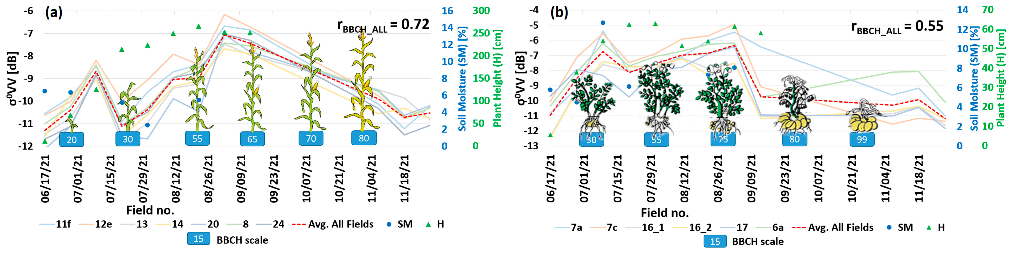
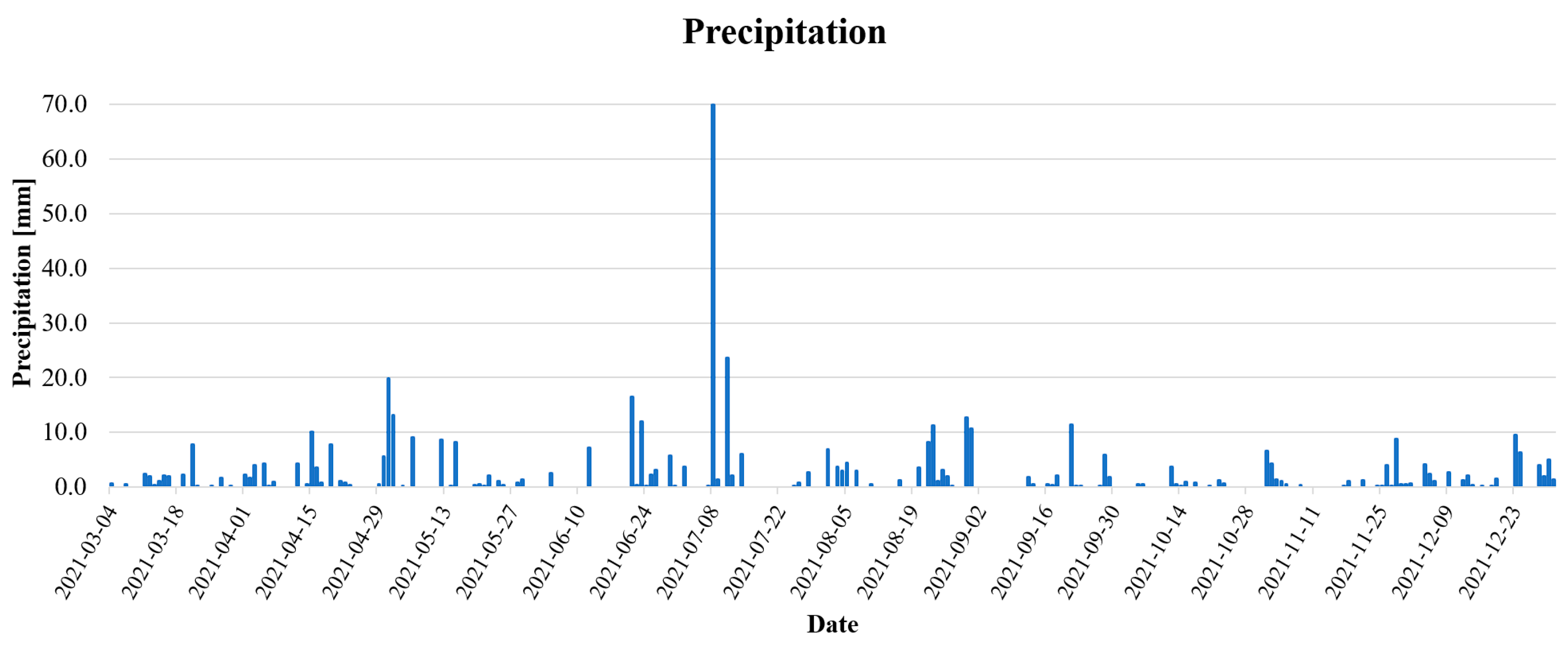
Depending on the plant species being studied, the ${\sigma }_{VH}^0$ behaves very differently. In the case of potato fields (Figure 6a), the lowest values overlap with the germination of the plant (BBCH0-15), which is around mid-May. However, a small peak can be observed which can be caused by soil moisture fluctuation. Regretfully, field data regarding soil moisture have not yet been collected for this period, but when observing the precipitation chart (Figure 5), during this time no significant precipitation appears. At the stages of development when the potato is growing in height and flowering, there is a very large increase in the value of the ${\sigma }_{VH}^0$ (BBCH20+). Such a moderate growth persists until BBCH70. When the plant turns yellow and falls to the soil (BBCH80-100), values drastically decrease, reaching their minimum peak around BBCH99, which perfectly captures the harvesting moment.

When observing height values and ${\sigma }_{VH}^0$, similar behavior as with BBCH development can be seen. Although the height of the plant has reached its maximum and does not change anymore, the index values start to decrease. This can be an indicator that leaves and other plant structures start to dry up and decline and the volumetric scattering starts to decrease at that time.

Nevertheless, the ${\sigma }_{VH}^0$ index corresponds with phenology development rather fairly, which is also reflected in the correlation index (r = 0.84). Satisfactory results were also found for corn and canola fields (r = 0.79 and r = 0.76, respectively). For these species, there is also some connection with plant height (r = 0.61 for maize, r = 0.82 for canola, and r = 0.55 for potato).

Observing Figure 6b, it is clear that there is no connection between phenology development and ${\sigma }_{VH}^0$ for rye. At the 25–30 BBCH stages of rye development, when the plant starts to expand in height, a definite rise in value can be seen. The index value dramatically decreases at the end of May (around the 35 BBCH stage), which is surely not interconnected with the phenological development. At the beginning of July, the index values increase strongly, coinciding with the mowing of rye (around BBCH60). The values of the ${\sigma }_{VH}^0$ drastically decrease between the time the plant reaches its peak stage of maturity (85–99 BBCH), and only after the cover crop appears do they begin to rise again (mid- to late August). Correlation analysis confirmed that the behavior of this index is related to rye development to a very small extent (r = 0.33). A very low level of correlation was also observed for winter wheat fields (r = 0.49).

• VV Backscattering—${\sigma }_{VV}^0$

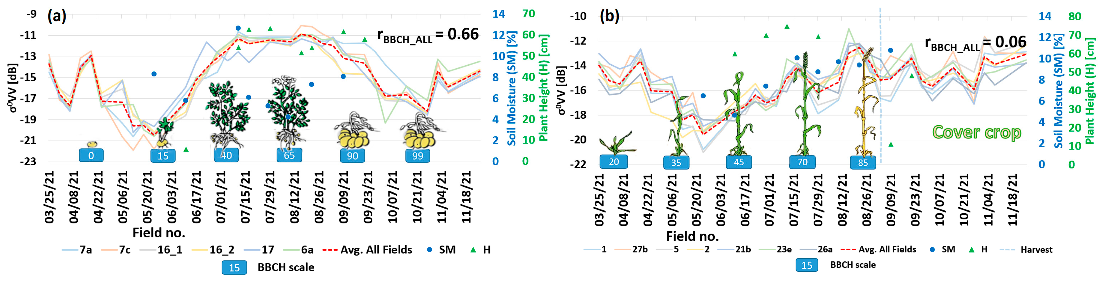
The ${\sigma }_{VV}^0$ coefficient’s usefulness in phenological stages’ tracking was not clearly visible. In the case of potato (Figure 7a), very significant noise can be observed during the period when the plant has not yet sprouted and bare earth was present. However, after late March to mid-May, the behavior of the index rather clearly reflects the phenological development of the potato (values lowest after germination, a significant increase during flowering). A fairly notable level of association with potato phenological phases was also observed in the correlation analysis (0.66); however, it was rather lower when compared with ${\sigma }_{VH}^0$.

The ${\sigma }_{VV}^0$ index shows a much lower level of correlation with wheat development (Figure 7b). Between phases 45 and 85 BBCH (late May to mid-August), there is a clear increase in value as winter wheat develops. However, the inability to determine the exact moment the plant was harvested is a serious drawback. It is also noteworthy that ${\sigma }_{VV}^0$ did not decrease after the harvest; in fact, it reached its highest values. The time series behavior of this coefficient for winter wheat fields also does not clearly indicate a link with the development of the cover crop. The unsatisfactory performance of the index is also confirmed by correlation index (r = 0.06).

The correlation analysis revealed that, while the ${\sigma }_{VV}^0$ coefficient does exhibit some phenological phase association, it does so to a far lesser extent than the ${\sigma }_{VH}^0$ coefficient. It would seem that, as crops mature, the value of the index should decline. However, the correlation for winter wheat is almost nonexistent and even approaches negative values in the case of some fields. For the other plants, the correlation level with phenological stages was r = 0.54 for corn, r = 0.55 for canola, and r = 0.11 for rye. A higher level of correlation was noted for plant height—in canola and potato fields, the correlation coefficient was 0.74 and 0.61, respectively, while the reverse correlation of r = −0.63 was observed for corn.

• DpRVI

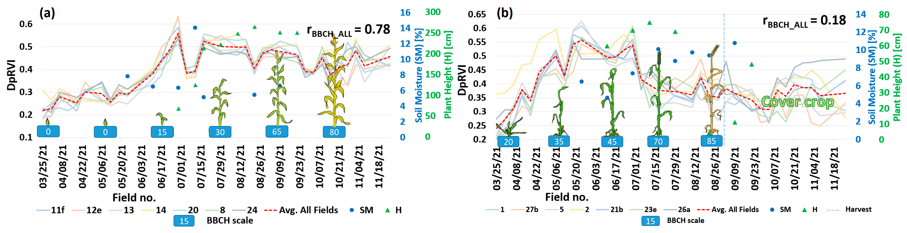
In Figure 8, the relationship between DpRVI and the phenological development for corn (Figure 8a) and winter wheat (Figure 8b) can be observed. The lowest values of these crops are observed during the periods of occurrence of the early BBCH phases. The fastest increase in values is observed in the BBCH30–35 for corn. From the 80 BBCH stage onwards (late September), the values of the DpRVI for this crop remain relatively constant. However, as the plant development progress further, the values begin to fluctuate. The correlation between phenological phases and corn achieved satisfactory results (0.78). Unfortunately, the DpRVI index does not indicate a strong correlation with plant height (−0.15) and soil moisture (−0.44) in this case.

Winter wheat (Figure 8b) exhibited the poorest correspondence with the vegetation index, similar to the previously mentioned indices. The variations in values were difficult to attribute to specific factors due to the high level of noise in the index values. In contrast, the index values for wheat increased until the 65–70 BBCH stage and then declined thereafter (early July). Significant changes in index values were observed after the plant reached maturity and was harvested, which could be indicative of exposed soil or the emergence of a cover crop. Correlation analysis for winter wheat indicated a low level of association with both phenological stages (0.18) and other field parameters (0.21 for height and −0.17 for soil moisture). In comparison, the results for another species such as potato and canola were unquestionably better, as shown in Table 2.

• Inverse of interferometric coherence $inv\left(\gamma \right)$

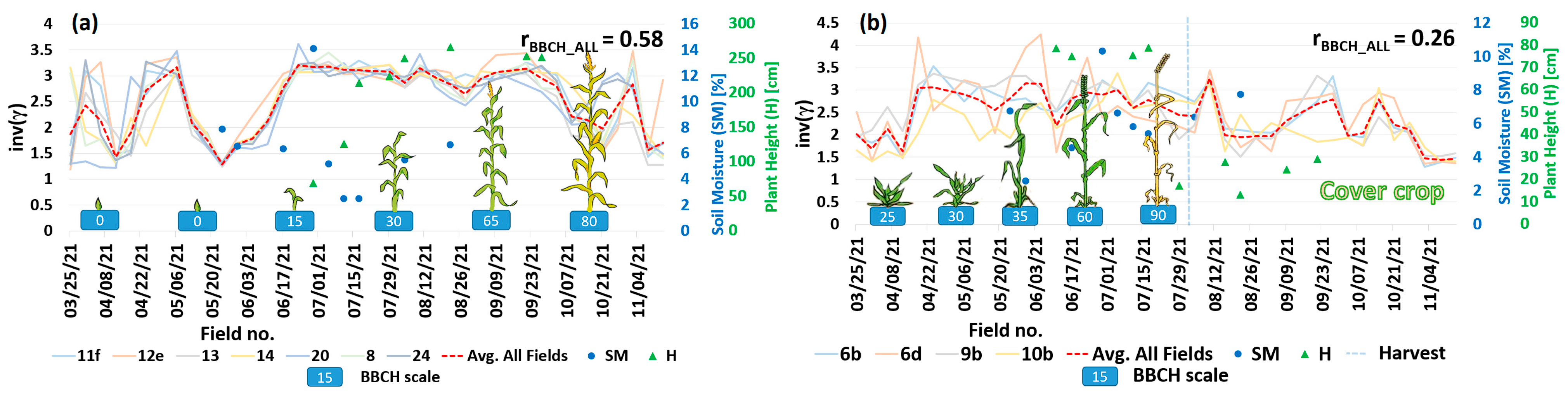
The correlation between the coherence and phenological phases of plants was not significantly high. The coherence values exhibited a considerable amount of noise, making it challenging to attribute variations in the values to specific phenomena. Only in the early phenological stages of corn, some speculations could be made regarding the onset of plant development. A noticeable increase in coherence values was observed between the 0-15 BBCH stages, corresponding to the germination and sprouting of corn’s first leaves (mid-May to mid-June). However, the $inv\left(\gamma \right)$ remained relatively constant thereafter, with occasional abrupt spikes and dips in early October. Correlation analysis revealed a close correspondence between coherence and phenological stages (0.58) and plant height (0.57). In contrast, the correlation with soil moisture was close to zero (−0.05).

The results are least favorable (r = 0.26) for rye fields (Figure 9b). The achieved signal exhibited a significant amount of noise, making it impossible to establish a significant relationship with field parameters. Although there are many noises, it is possible to discern that the potato’s maximum values are around the 65 BBCH stage, when it is in the flowering stage, but extremely large fluctuations start to show as the potato reaches maturity (the 90–99 stage). Correlational analysis (Table 2) revealed a moderate correlation between the coherence estimated for corn, canola, and potato fields and the phenological phases (the mean r values for corn, canola, and potato were 0.58, 0.51, and 0.50, respectively), as well as the height of corn and canola (mean r values of 0.56 and 0.51, respectively). In contrast, winter wheat fields show a moderate degree of relationship with natural soil moisture (inverse correlation at r = −0.36) and phenological stages (r = 0.38).

3.2.2. Terra-SAR-X-Delivered Indices

• Backscattering ${\sigma }_{VH}^0$

Due to the fact that TSX data are not freely available, the creation of a consistent time series was severely limited, making it impossible to observe the complete life cycle of certain plant species from sowing to harvesting. This limitation posed a significant challenge in establishing a connection between the SAR signal and plant growth, potentially impacting the findings of the correlation analysis.

In the case of corn (Figure 10a), a gradual increase in values was observed between the 30 and 65 BBCH stages. However, ${\sigma }_{VH}^0$ started to decline as the plant matured (at stage 70 BBCH and beyond). This significant decrease appears just after corn flowering, when the canopy starts to decay. It is noteworthy that the ${\sigma }_{VH}^0$ values did not exhibit the same abrupt changes as in the case of Sentinel-1 data during the autumn period (November). In potato fields (Figure 10b), an increase in ${\sigma }_{VH}^0$ was observed as the phenological stage progressed (55–80 BBCH stages). The coefficient’s value significantly dropped once the potatoes reached full maturity, the plants dried up, and collapsed to the ground (late September to early October). On 7 September 2021, a single increase in value was observed for corn. This increase may be attributed to the maximum soil moisture content observed during this period, with an average of 14.04% for corn fields and 12.70% for potato fields. With the exception of rye fields, the correlation analysis (Table 2) indicated a strong association between the ${\sigma }_{VH}^0$ coefficient and the phenological phases of the plants. Unlike the Sentinel-1 data, a correlation between this indicator and wheat development was identified (average r = 0.72), although it should be noted that this result only considers the plant’s final phenological stages. The correlation indices for corn and potatoes with phenological stages were 0.81 and 0.68, respectively. Despite the negative correlation (r = −0.68), the coefficient values for canola fields also exhibited a significant degree of association with plant growth. However, it is important to keep in mind that this dataset only allows for the observation of the latter phenological stages of these plants.

• Backscattering ${\sigma }_{VV}^0$

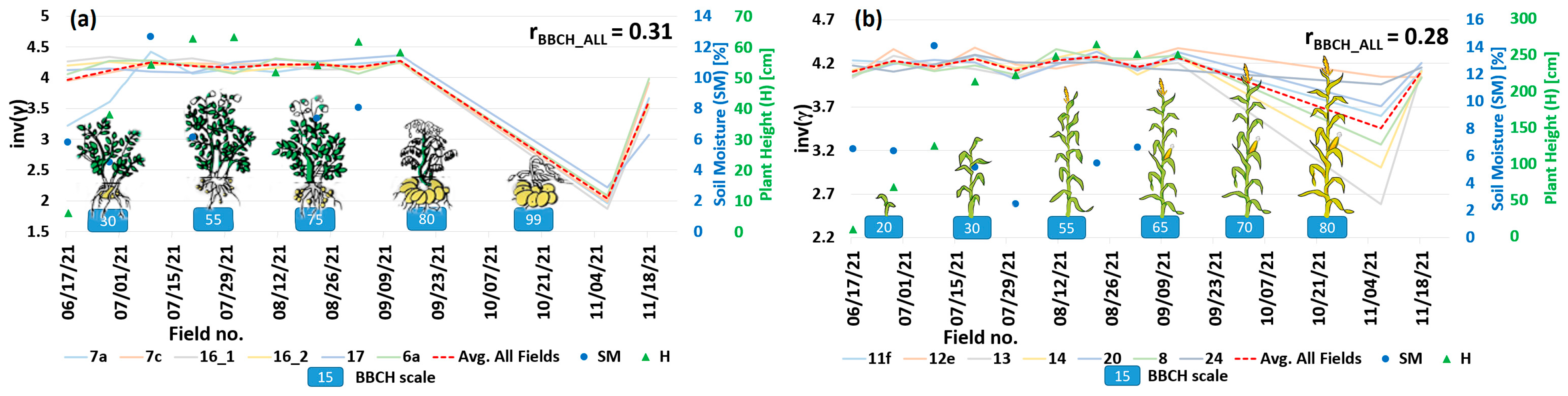
The analysis of ${\sigma }_{VV}^0$ in TSX data revealed that it exhibited a similar behavior to the ${\sigma }_{VH}^0$ index, with increases and decreases occurring at similar time periods for all crops. The only meaningful differences were observed in the values calculated for corn (Figure 11a) and canola. In the case of corn, there was a wider disparity in the index values among the fields compared to the ${\sigma }_{VH}^0$ index. The correlation analysis (Table 2) using field data indicated that the ${\sigma }_{VV}^0$ index was most closely associated with the phenological stages of the plants. Although the results are not particularly high compared to the ${\sigma }_{VH}^0$ index, a certain level of correlation (r = 0.64) between the ${\sigma }_{VV}^0$ index and the phenological stages of rye was detected.

Correlations were found for corn, wheat, and potatoes (Figure 11b) at levels of 0.72, 0.96, and 0.42, respectively, and for canola at a level of −0.62 for inverse correlation. Similar to the ${\sigma }_{VH}^0$ index, it should be noted that these correlation coefficients were obtained for plants in which only the later stages of their development could be studied (winter wheat, rye, canola).

• DpRVI

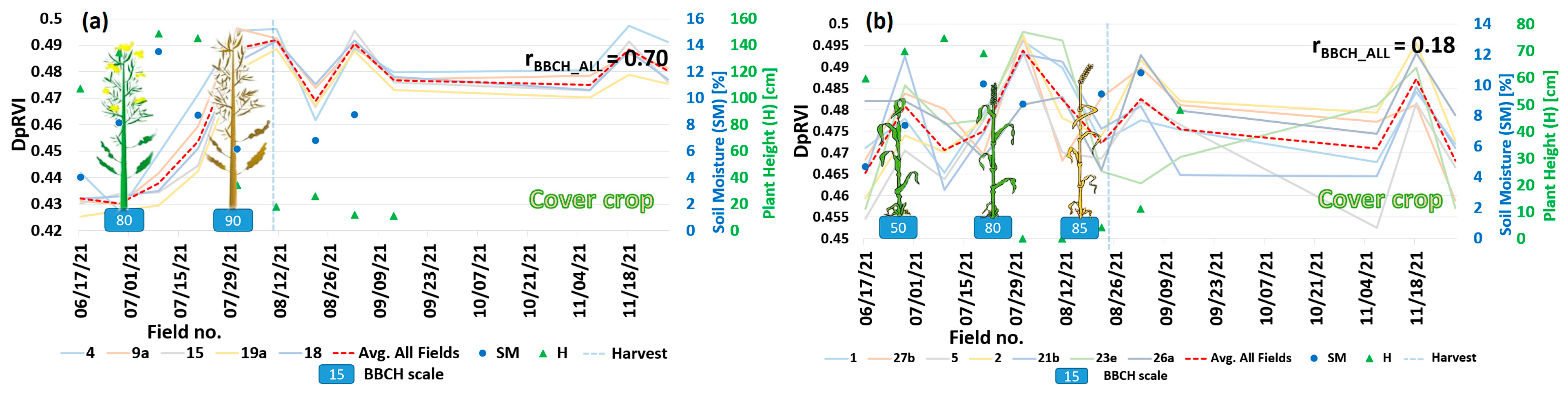
The DpRVI index calculated for the TSX data did not show the same potential as the ${\sigma }_{VH}^0$ and ${\sigma }_{VV}^0$ backscattering coefficients. There were multiple jumps in the values of this index for all plant species, which interfered with their readability and made it challenging to connect these values to plant development. This index showed the highest level of linkage for canola development (Figure 12a). Unfortunately, it was only possible to relate the last developmental stages of this plant due to the much smaller number of TSX images. The index reached its highest values when the plant was fully grown and ready for harvest. After the harvest was observed, DpRVI values decreased slightly, followed by an increase. It is likely that this behavior was a signal response to the occurrence of cover crop in the crop fields. Correlation analysis (Table 2) also indicates that the DpRVI index is linked to the height of the canola plant (r = −0.81).

The DpRVI index failed to depict behavior that may arise as a result of winter wheat entering subsequent stages of development (Figure 12b). Additionally, the correlation analysis failed to provide a clear explanation of how the index may be related. In addition to variety between species, the values of the r coefficient also varied within specific fields. The DpRVI index calculated for winter wheat reached the lowest association level with phenological phases (r = 0.18). The results for other plant species are shown in Table 2.

• Inverse of Coherence $inv\left(\gamma \right)$

Coherence had the lowest outcomes of all the indices and coefficients derived from the data in the correlation analysis. Throughout most of the potato growth period (Figure 13a), coherence remained consistently stable, with only minimal fluctuations in values. Decreases in values were observed exclusively when the plant was ready for harvest (i.e., it was dried and fell to the soil). For soil moisture and plant height, the coherence showed no significant level of correspondence (0.25 and 0.28, respectively).

Coherence behavior was very similar in the case of corn (Figure 13b). Throughout the development period, values remained at similar levels, and a decline was observed only when the corn began to reach maturity. Correlation analysis did not show a significant degree of association with the other field parameters (0.33 for height and −0.18 for soil moisture). The one exception is canola (Table 2), where plant harvesting caused a visible drop in coherence values. In cultivated areas, even those sowed with the same plant species, the values of the r coefficient varied extremely significantly. This made it impossible to relate coherence to any of the known plant parameters or soil moisture.

3.3. Temporal Time Series Filtering

In Figure 14, the graphical representation of the temporal filtering methods is presented. As can be observed, in general, both methods allow for smoothing the acquired signal and increasing the correspondence with phonological development phases captured in the field. However, various window sizes of the filtering influence the final correlation results. Specifically, a wider window size allows for a higher smoothing effect and, in most cases, achieves better correlation results. This is mainly due to filtering out some of the other backscattering contributions not related to phenological development, such as soil moisture or soil roughness.

The moving average (MA) method provides N-M-filtered values (N—number of observations, M—window size), which results in the shortening of the time series at the beginning of the observed time. Therefore, this filtering method can be applied to longer time series with some additional observations before the investigated time to achieved full time series for investigated period. In the case of Savitzky–Golay (SG) filtering, such shortening of the time series is not preserved, making SG more appropriate for agricultural monitoring. On the other hand, a higher polynomial degree in SG allows for a better fit of the model into the time series dataset. However, when some noise (non-vegetation-related contributions) is preserved in the time series, the filtered signal also represents that noise. Therefore, in the case of numerous other backscattering contributions that do not correspond to the phenological development, lower orders of the polynomials should be used.

Table 4. An example of correlation changes for some plant species achieved by various filtering methods and their parameters (window size or poly order) in the context of height (H) and phenology stage (BBCH) in the form of heatmap.

	Sentinel-1
SAR Derivatives	${\mathit{\sigma }}_{\mathit{V}\mathit{H}(\mathit{S}\mathit{G}=15)}^0$—H			${\mathit{\sigma }}_{\mathit{V}\mathit{H}(\mathit{S}\mathit{G}=15)}^0$—BBCH
Poly order	3	2	8	3	2	8
Corn (BBCH BBCH0-80)	0.82	0.89	0.77	0.90	0.92	0.83
Winter wheat (BBCH BBCH21-100)	−0.14	−0.40	−0.03	0.60	0.76	0.57
Canola (BBCH26-100)	0.84	0.84	0.92	0.92	0.95	0.84
Potato (BBCH0-96)	0.65	0.72	0.74	0.85	0.90	0.89
Rye (BBCH24-100)	−0.10	−0.40	−0.09	0.60	0.83	0.37

presents how correlation parameters change according to the various parameters used. It can be observed that, in some cases, significant increases and decreases in correlation can be found.

4. Discussion

4.1. Effectiveness of Radar Indices in Phenological Stages Monitoring

When analyzing temporal time series and BBCH phases, strong correspondences between phenological phases and SAR-delivered signals are observed, especially in those phenological stages when plants are growing and undergoing structural changes (BBCH 10–70). In the very early stages of vegetation, strong contributions from soil and water content are observed, which directly affect the correlation between SAR signal and BBCH stages. This can also be seen in the Pearson correlation values for some plant species, such as winter wheat. A statistically moderate correlation can be observed between ${\sigma }_{VH}^0$ or DpRVI and soil moisture (r ≈ 0.5). However, when observing

Table A2. Correlation indices for winter wheat before temporal filtering, after Savitzky–Golay (SG) filtering (window size 15) calculated for ${\sigma }_{VV}^0$, ${\sigma }_{VH}^0$, DpRVI index, and interferometric coherence (inv(γ)) from Sentinel-1 in the form of heatmap. Bold font represents the highest correlation index between specific SAR vegetation index and in situ data of vegetation height (H), soil moisture (SM) and phenology development in BBCH scale.

	Winter Wheat
	${\sigma }_{VH}^0$			${\sigma }_{VH\left(SG\right)}^0$			${\sigma }_{VV}^0$			${\sigma }_{VV\left(SG\right)}^0$
Field No.	H	SM	BBCH	H	SM	BBCH	H	SM	BBCH	H	SM	BBCH
1	0.23	0.15	0.32	0.26	0.24	0.34	0.00	0.39	0.06	0.47	0.54	−0.11
27b	−0.09	0.72	0.66	−0.38	0.69	0.72	0.55	0.64	−0.10	0.75	0.68	−0.30
5	0.09	0.10	0.22	−0.25	0.72	0.08	0.32	0.37	0.01	0.61	0.74	−0.12
2	−0.09	0.24	0.19	−0.32	0.82	0.74	0.36	0.60	0.22	0.51	0.72	0.30
21b	0.03	0.65	0.66	0.02	0.63	0.82	0.60	0.82	−0.04	0.69	0.85	−0.15
23e	0.26	0.49	0.69	−0.10	0.53	0.70	0.35	0.64	0.13	0.68	0.38	0.01
26a	−0.15	0.46	0.67	−0.25	0.37	0.81	−0.04	0.27	0.15	0.13	0.27	0.19
All Fields	0.04	0.40	0.49	−0.14	0.57	0.60	0.30	0.54	0.06	0.55	0.60	-0.03
	DpRVI			DpRVISG			inv(γ)			inv(γ)SG
Field no.	H	SM	BBCH	H	SM	BBCH	H	SM	BBCH	H	SM	BBCH
1	−0.39	−0.54	0.05	−0.58	−0.56	0.20	0.60	−0.36	0.41	0.32	−0.74	0.54
27b	−0.75	−0.54	0.52	−0.74	−0.56	0.60	0.04	−0.53	0.36	0.76	−0.69	0.55
5	−0.66	−0.51	0.02	−0.63	−0.67	0.08	0.43	−0.27	0.42	0.30	−0.62	0.40
2	−0.35	−0.79	−0.25	−0.64	−0.68	−0.06	0.38	−0.64	0.47	0.34	−0.72	0.46
21b	−0.80	−0.73	0.32	−0.78	−0.84	0.35	−0.42	−0.40	0.18	0.72	−0.74	0.40
23e	−0.39	−0.63	0.22	−0.75	−0.30	0.39	0.19	−0.12	0.54	0.73	−0.43	0.61
26a	0.12	−0.15	0.36	0.05	−0.28	0.30	−0.55	−0.18	0.31	−0.50	−0.25	0.50
All Fields	−0.46	−0.56	0.18	−0.58	−0.56	0.27	0.09	−0.36	0.38	0.38	−0.60	0.49

in Appendix A, various correlations are represented for different fields (0.1–0.72). This could be attributed to variations in vegetation biomass or crop coverage. For example, when fewer plants are sown, resulting in lower crop coverage, a greater proportion of backscatter comes from the soil. Nonetheless, for all plant species, there is a significant decrease in values in the later stages of plant development (BBCH 80+), which is also connected to structural changes such as leaf withering and reduction in green mass. Various indices show that, during the initial stages of the vegetation period, values increase or decrease and reach their maximum or minimum during the booting stage. Time series profiles have the advantage of reflecting the timing of barley head bending [39]. Mercier et al. (2020) [33] also observed highly varying polarization during stem elongation due to heterogeneous plant structures, as indicated by increasing Shannon entropy. Surprisingly, potato fields show a high correlation with SAR-delivered indices, although it was expected that corn, due to its height, would exhibit the highest volumetric scattering and therefore be the most correlated with the SAR response. Another factor that could affect the high correlation achieved for potatoes (in addition to soil moisture and vegetation water content) is surface roughness, which is also considered a significant contribution to backscattering [40,41].

Depending on the type of plant being monitored, the radar indices and coefficients computed from Sentinel-1 and TerraSAR-X data have various sensitivities. The process of development of these crops looks rather different, and the entry into the next stages of development took place at different times depending on the plant species, which could affect the behavior of the remote sensing radar signal. For instance, compared to the other species, the correlation between the development of rye and wheat and the ${\sigma }_{VV}^0$ and ${\sigma }_{VH}^0$ indices derived from S1 data is rather low. The same indices calculated from TSX data, revealed a substantially higher degree of association with wheat development. On that basis, it may be concluded that various radar signal frequencies may exhibit varying sensitivity to various crop species.

The high amount of noise present in the computed indices proved to be a significant challenge when monitoring the phenological stages of crop plants. Significant fluctuations in data values, characterized by rapid spikes and dips, introduced a notable level of noise in the correlation between phenological stages and the rest of the in situ data for certain species. Depending solely on these data could potentially lead to multiple errors in interpretation. To pinpoint the sources of these inconsistencies, we collected additional information on soil moisture and plant height. However, in the majority of cases, these factors did not exhibit a significant disruptive effect on the results.

In some fields, we observed varying degrees of contamination by weeds. This occurrence might have caused the radar remote sensing signal to capture data not only from the target plant species but also from other, unidentified species. Despite our efforts during the field selection process to exclude heavily weed-infested areas from the experiment, in certain instances, particularly in expansive fields, weeds may have been located in areas that were challenging to identify during field inspections.

4.2. Effect of Filtering on the Degree of Correlation between Radar Data and Phenological Stages

Temporal filtering methods effectively smooth the signal and are beneficial for noise removal in time series analysis. Depending on the filter window’s size and the vegetation index being filtered, different results were obtained. Using a larger polynomial order in SG filtering produces filtered values that closely resemble the original signal. On the other hand, the MA method may result in a shortened time series observation, especially with larger window sizes. Therefore, for the MA method, neighboring time series observations are needed. In this context, SG methods is more recommended. However, in some cases, different window sizes allow for better correspondences with the in situ data. Generally, wider window sizes provide a better smoothing of the signal and limit the effects caused by temporal decorrelation or other non-BBCH-related aspects such as soil moisture, vegetation water content, vegetation coverage, and biomass.

5. Conclusions

The goal of this study was to evaluate the behavior of the C-band (Sentinel-1) and X-band (TerraSAR-X) radar signals to investigate their efficacy in the context of tracing the phenological phases of crop plants. The obtained results from various SAR vegetation indices were cross-referenced with information about soil moisture, plant height, and the phenological stages estimated in BBCH scale. To reduce the impact of noise or information which is caused by other non-phenological aspects (soil moisture, decorrelation, water content), various temporal filtering methods with various parameters were analyzed.

According to a correlation analysis of radar indicators with field measurements, S-1 as well as TSX data have a very high potential for tracking agricultural development. A rather good degree of correlation between the C-band signal and the development of the majority of plants was already attained without the use of filtering. After comparing the results of S-1 and TSX (X-band) data from the same time series, the X-band also showed clear potential in monitoring plant development. In some instances, higher correlation coefficients with field parameters were found with some plant species using this type of data (e.g., corn and potato). The viewing geometry and incidence angle may have been a factor that influenced the results since TSX and S-1 were acquired from different geometries. However, different times of data acquisition between S-1 and TSX could also cause such effect. The rather short time series that prohibited the study of major phenological phases of some plant species is significant to mention despite the positive results achieved by the TSX data. Future studies should create a long and consistent time series spanning the full growth stage of the plants being observed to better comprehend the X-band signal. Moreover, for a better comparison between S-1 and TSX, data from similar viewing geometry should be considered. The greatest analytical outcomes for Sentinel-1 as well as TSX data were backscattering coefficients, particularly the ${\sigma }_{VH}^0$ coefficient. Interferometric coherence and DpRVI present smaller performance.

The potential of SAR data for plant monitoring was increased by the time series filtering. Even for indices that produced incredibly subpar results, SG filters and moving average greatly boosted the correlation level of the Sentinel-1 signal. The SG filter in a window of size 15 was the best in this regard, raising the correlation level of the ${\sigma }_{VH}^0$ coefficient even above 0.90 in individual cases (S-1). Although higher correlation values were obtained after using a moving average in a window of size 9, this type of filtering cuts off a portion of the data at the beginning of the time series, which makes it impossible to monitor crops from sowing to harvest. For TSX data, however, this filter was utterly useless. The key determining factor was the volume of data collected; due to the relatively limited number of TSX images, it was nearly impossible to control the filter’s window, severely restricting its usefulness. However, it can be foreseen that, for a higher number of TSX data, such time series filtering should also be beneficial. The SG filter was clearly preferable in the case of such a small dataset, but the outcomes were still inferior to those derived from S-1 data.

The results of this experiment suggest that SAR data may one day be used to remotely monitor crop plants, however still more studies is needed to define which index and which sensor should be used for specific species and how other components such as surface roughness, soil and vegetation water content contribute to the changes of the index. Creating a long, uniform time series that spans the whole period of plant development and using the right filtering to reduce the impact of another components are the key factors to increase SAR efficacy in vegetation monitoring.