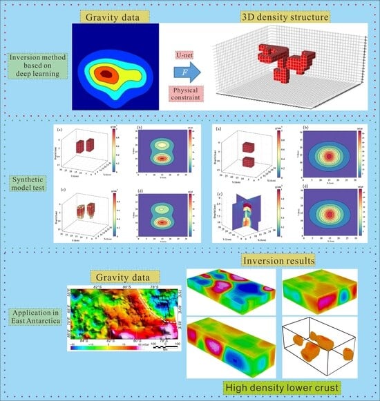
Improved Gravity Inversion Method Based on Deep Learning with Physical Constraint and Its Application to the Airborne Gravity Data in East Antarctica

Abstract

This paper aims to solve the limitations of traditional gravity physical property inversion methods such as insufficient depth resolution and difficulties in parameter selection, by proposing an improved 3D gravity inversion method based on deep learning. The deep learning network model is established using the fully convolutional U-net network. To enhance the generalization ability of the sample set, the large-scale training set and test set are generated by the random walk, based on the forward theory. Founded on the traditional loss function’s definition, this paper introduces an improvement incorporating a physical constraint to measure the degree of data fitting between the predicted and the real gravity data. This improvement significantly boosted the accuracy of the deep learning inversion method, as verified through both a single model and an intricate combination model. Finally, we applied this improved inversion method to the gravity data from the Gamburtsev Subglacial Mountains in the interior of East Antarctica, obtaining a comprehensive 3D crustal density structure. The results provide new evidence for the presence of a dense crustal root situated beneath the central Gamburtsev Province near the Gamburtsev Suture.

1. Introduction

As an important method in geophysical interpretation, gravity inversion can be used to determine the nature of mass distribution and identify anomalous fields, finding extensive applications in various domains such as natural resource survey, bedrock topography mapping, and global plate tectonic studies [1,2,3].

The traditional gravity inversion involves uniformly dividing the subsurface space into multiple prisms, each characterized by defined physical parameters. Subsequently, a suitable objective function is established to obtain the inversion results. During this process, priori information and constraints are utilized to reduce the non-uniqueness of the inversion results [1,4]. The inversion process is to minimize the objective function, commonly used algorithms such as the least squares fitting method, gradient descent method, Newton’s method, conjugate gradient method, etc. The issue of algorithm selection has posed a challenge due to variations in their performance concerning inversion speed and outcomes. The inversion problem typically suffers from issues such as insufficient resolution and non-uniqueness. To address these challenges, constraints were introduced to the model in the objective function and used regularization to improve the inversion results [5]. However, a significant concern arises from the profound decay of the kernel function with depth leading to the inversion results clustering near the surface, referred to as the skinning effect. To tackle this problem, a depth-weighting function was introduced into the objective function of the inversion algorithm utilizing a spatial derivative as a constraint [1,6]. Last and Kubic (1983) introduced a minimum volume constraint in the objective function, leading to inversion outcomes with more explicit bounds [7]. To address the dispersion in inversion results, Portniaguine and Zhdanov (1999) proposed a 3D focused inversion algorithm utilizing the minimum gradient support (MGS) functionals in combination with the penalization function [8]. Zhang et al. (2018) obtained the 3D density structure distribution on the lunar surface through full-gravity gradient tensor inversion using the Gauss–Legendre integral method [9]. However, implementing 3D inversion requires a substantial allocation of computing time and storage capacity. Subsequently, numerous advanced techniques have been proposed. These include the utilization of cubic interpolation [10], wavelet transforms [11], and adaptive sampling of potential data [12] to compress the function. These approaches have greatly accelerated the speed of inversion calculations and gained extensive adoption.

As a new branch of machine learning, deep learning has shown excellent performance in recognition and classification for image processing, particularly in handling inverse problems like model reconstruction. This allows computer systems to train and learn from vast quantities of data. Unlike conventional geophysical inversions, deep learning-based inversion approaches rely on data-driven methodologies to map observed data to a 3D physical property model [13]. Due to its superior performance, deep learning-based inversions are widely used in geophysical data processing and inverse problems, including seismic [14,15,16], electromagnetic [17,18,19], gravity, and magnetic [13,20,21,22,23,24]. Moreover, deep learning algorithms are also utilized for the joint interpretation of geophysical data through the integration of unsupervised cluster analysis and supervised classification, enhancing the coherence of the obtained solution [24]. Huang et al. (2021) proposed a new 3D sparse inversion method for gravity data based on deep learning, which was validated using real gravity data [25]. By utilizing the random walk method, the network’s generalization ability of the network can be improved [25,26]. To estimate the depth of the sediment–basement interface, He et al. (2021) explored a novel approach using convolutional neural networks (CNNs) for direct depth-to-basement inversion from gravity data. Moreover, CNNs are used to detect the impact craters from GRAIL-acquired gravity data [27]. Collectively, these studies provide new perspectives for reconstructing density models from gravity data and highlight the considerable potential of deep learning in the domain of gravity inversion. However, the absence of a constraint term in the loss function leads to poor utilization of all the observed data. Currently, the incorporation of additional constraint information into the inversion process poses a significant challenge for the 3D physical property inversion of potential field data. With the advancements in deep learning, enhancing data-driven deep learning techniques is imperative to achieve more accurate outcomes, thereby highlighting the importance of integrating constraint information [13,23].

This paper presents an improved 3D gravity inversion method based on deep learning. Specifically, a gravity data inversion network model is developed using the U-net neural network architecture. A large-scale dataset is constructed by using the random walk method based on the gravity forward theory. The traditional loss function is improved by incorporating a physical constraint term, which characterizes the level of fitting between the real measured and predicted gravity data. The effectiveness of this improved inversion method is demonstrated through synthetic models. Finally, this method is applied to the airborne gravity data obtained in the interior of East Antarctica, resulting in the estimation of 3D crustal density structure.

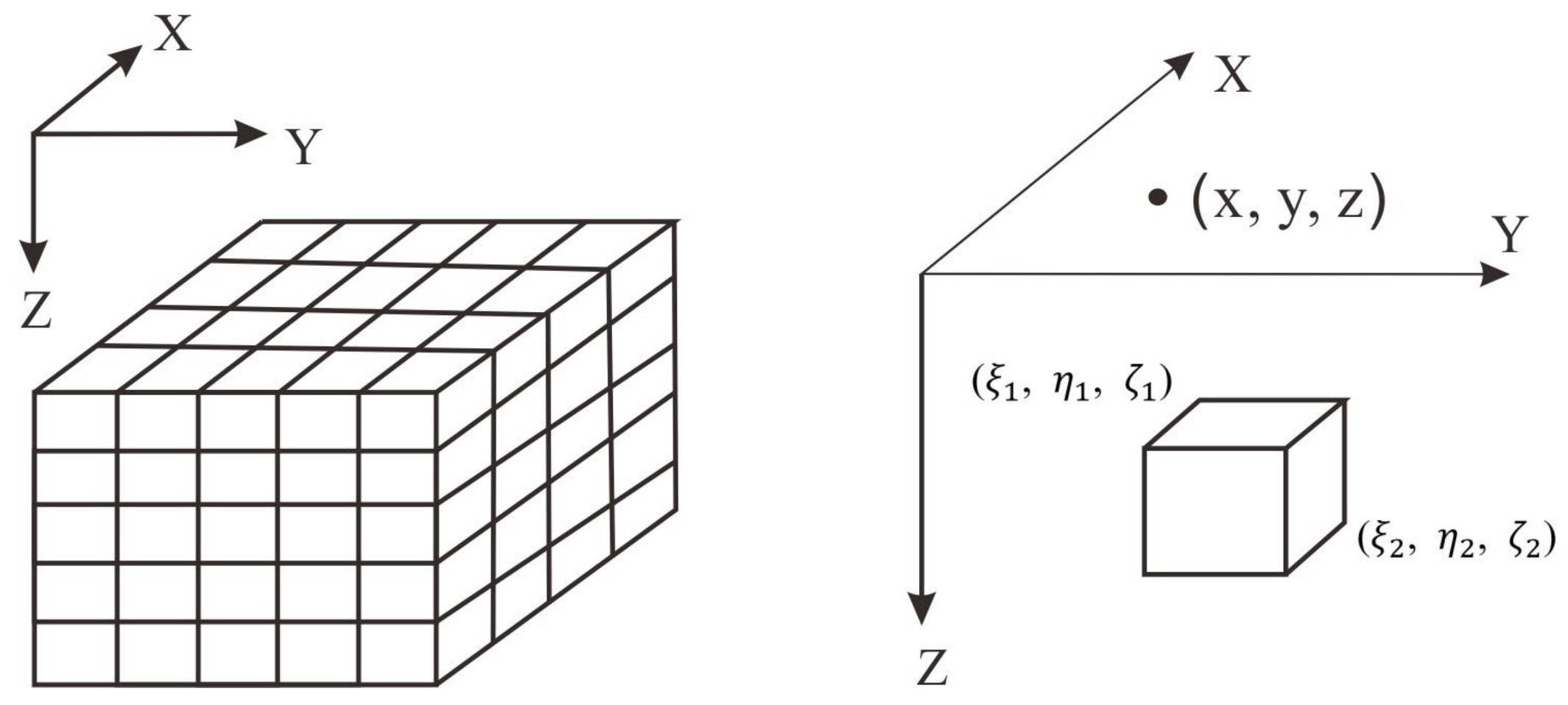
2. Forward Modeling of Gravity Anomalies

The forward modeling serves as the foundation for solving the inversion problem, obtaining the anomaly observed at a specific point through theoretical forward calculation. This is achieved by using the positional shape and physical property parameters of the underground source.

The underground space within the study area is divided into regular prisms, as shown in Figure 1. This implies that the underground model space is uniformly divided into N prisms, each with a specific size and a different density value. The calculations are conducted within a Cartesian coordinate system, with the X and Y axes denoting the eastward and northward directions, respectively, while the Z axis represents the vertical underground direction. The resultant gravity anomaly generated by the underground sources at the observation point is the sum of the gravity anomaly generated by all subdivision prism units at the observation point. For a given observation point (x, y, and z) situated on the ground surface, the gravity anomaly attributed to each prism can be mathematically expressed as [28,29,30]

$$\mathrm{g}=-\gamma {\rho }_j{\displaystyle \sum _{p=1}^2{\displaystyle \sum _{q=1}^2{\displaystyle \sum _{s=1}^2{\mu }_{pqs}\times \left[a_p\ln \left(b_q+r_{pqs}\right)+{\mathrm{b}}_q\ln \left(a_p+r_{pqs}\right)-c_s\arctan \left(\frac{a_p{\mathrm{b}}_q}{c_s{r}_{pqs}}\right)\right]}}}$$

(1)

where, ${\mu }_{pqs}={(-1)}^{pqs}$, p, q, s = 1, 2, $a_p=x-{\xi }_p$, $b_q=y-{\eta }_q$, $c_s=z-{\zeta }_s$. $\mathrm{\gamma }$ represents the gravitational constant, ${\rho }_j$ denotes the residual density, and $r_{pqs}$ denotes the distance from the corner of the prism to the observation point, $r_{pqs}=\sqrt{a_p^2+b_q^2+c_s^2}$. The gravity anomaly at the observation point can be expressed as the sum of anomalies generated by all prisms underground, namely,

$$\mathrm{g}={\sum }_{j=1}^N{G}_j{\rho }_j$$

(2)

where $G_j$ represents the kernel matrix. The above formula can also be written as

$$\mathrm{d}=Gm$$

(3)

where d represents the observed gravity data vector, and m represents the model density contrast value vector.

3. Gravity Inversion Based on U-net Network

Gravity inversion involves solving the inverse problem through forward modeling. In this process, the positions, shapes, and physical parameters of underground bodies are calculated from observed data.

The inversion problem can be expressed as

$$m=M\left(d,\theta \right)$$

(4)

where $M$ represents a mapping relation, signifying the underground density model can be derived from the input data, with $\theta$ representing the parameters obtained during the inversion process.

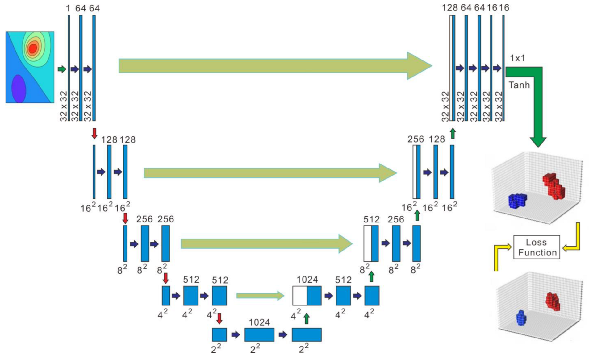
3.1. Introduction to U-net Network

With the rapid advancement of computer technology in recent years, deep learning has emerged as a prominent area of research. Its essence lies in training established network structures using an extensive dataset, enabling the learning of the representation level and internal rules of the sample data. Ultimately, this process endows the network with humanlike learning and analytical capabilities, enabling the interpretation and recognition of diverse data modalities, such as text, sound, and images. In this study, the U-net network architecture is employed for deep learning, complemented by the generation of a forward gravity data sample set for network training. Once satisfactory training results are achieved, authentic data are inputted to predict the underground density model using the network. As shown in Figure 2, the U-net network embodies a typical fully convolutional network (FCN), resembling the shape of the letter “U”. Comprising two main segments, the left part constitutes the feature extraction layer, known as the encoder, while the right part encompasses the up-sampling process, known as the decoder.

The left side of the network comprises a series of down-sampling processes involving convolution and pooling. This section includes four submodules, each housing two convolution layers. Each submodule achieves down-sampling through convolution operations using a 2 × 2 convolution kernel of with a step size of 2. Moreover, a dropout layer is added to minimize overfitting. In this study, a single channel of gravity anomaly data with a resolution of 32 × 32 was used as the input, which corresponded equivalently to 1024 observation stations evenly distributed across the ground. Following two convolutional layers, the channel count expands to 64. The resolutions of modules 1–5 are successively 32 × 32, 16 × 16, 8 × 8, 4 × 4, and 2 × 2 with the channel count of the former being half of that in the latter. This segment of the network parallels a standard CNN, using a 3 × 3 convolution kernel to capture the implicit relationships between pixels within the image.

The decoder mirrors the structure of the encoder and contains four modules. It symmetrically magnifies features through up-sampling, gradually aligning the output resolution with that of the input image. Simultaneously, the network uses jump connections to connect the up-sampling outcome from the submodule of equivalent resolution in the encoder. During this process, the number of data channels is halved, and the size is doubled. This linked result is input for the next submodule in the decoder, to obtain more accurate information and achieve better results. Finally, an activation function is applied to predict each pixel’s value in the channel, generating the predicted subsurface density model. The expression and pattern of the Tanh function are shown in Figure 3.

3.2. Improvement of Loss Function

The U-net network employs supervised deep learning. Fundamentally, when provided with training samples and their corresponding labels, it endeavors to grasp the mapping relationship between samples and labels. Specifically, it seeks to discern the mapping relationship between the anomaly data and the density contrast model. The training process aims to minimize the disparity between the network’s output and the real model, necessitating a function to quantify the distinct or level of alignment between the output and the actual values.

The loss function is an operational measure used to characterize the difference between the network’s output and the actual values. A smaller loss function signifies the greater reliability of the network model. During the model’s training stage, forward propagation is used to calculate the output of each batch input. Subsequently, the model’s predicted values are generated. The loss function then qualifies the distinction between these predicted values and the actual values, accomplished through a specified activation function, resulting in a loss value. Upon obtaining the loss value, the model initiates backpropagation to adjust updates each parameter within the network. This adjustment process aims to minimize the disparity between the predicted and actual values, effectively reducing the loss. The model iteratively refines these parameters to bring the calculated predictions closer to actual values, thereby achieving the goal of learning.

Huang et al. (2021) introduced the Dice function, which quantifies the fitting degree of the prediction model and the real model [25]. This function denoted by the Dice function operates within a range of 0–1, representing the degree of similarity between the two models. A higher value denotes a greater degree of similarity. Therefore, the loss function in this paper is expressed as follows:

$$\mathrm{L}=1-\mathrm{D}\mathrm{i}\mathrm{c}\mathrm{e}\left({\widehat{m}}^i,m^i\right)$$

(5)

where ${\widehat{m}}^i$ and $m^i$ represent the prediction model and the actual model, respectively. To enhance the loss function, this paper modifies it by adding a constraint term representing the degree of data fitting:

$$\mathrm{L}=\alpha \ast {‖{\widehat{m}}^i-m^i‖}_{L2}^2+{\beta \ast ‖{\widehat{d}}^i-d^i‖}_{L2}^2$$

(6)

where $\alpha$ and $\beta$ are the weights and ${\widehat{d}}^i$ and $d^i$ are the gravity anomaly data of the prediction model and the real model, respectively. In theory, a well-fitting predictive model should generate the anomalies that exhibit a commendable degree of correspondence. The incorporation of the anomaly data constraint not only optimizes the loss function but also optimally leverages the entirety of the available data.

3.3. Establishment of Sample Datasets

Once the training network has been set up, it is necessary to establish enough sample datasets for network training. Differing from the traditional supervised learning method that initially procures input image data and then manually labels it, this study follows an alternative path. Here the labels are synthesized before deducing the corresponding input data, in this case, the density model. Subsequently, the corresponding anomaly data are calculated.

The utilization of the deep learning method requires large-scale datasets for training. Its effect is intricately linked to the characteristics and circumstances of the dataset. To assess the feasibility and efficacy of the deep learning inversion method within the case of complex datasets, this study first commenced by using a random walk approach to generate 20,000 structured density models. The underground research area was uniformly divided into 32 × 32 × 16 = 16,384 cubes, each with 1 km side length. The underground density models were generated by using the random walk method. This method involves establishing an initial point within the space immediately and allowing it to move a certain number of steps in random directions. Figure 4a,b depict the models resulting from random walks of 10 and 30 steps, respectively.

Upon establishing the actual model, the residual density of the gravity source was set to 1 g/cm³, while the background was set to 0 g/cm³. Consequently, a density model was generated in an area of 32 × 32 × 16 km underground by dividing the model space into the same output size as the network structure. In the process of generating the underground density model using the random walk method, a 2 × 2 × 2 cube was initially designated as the starting point, followed by allowing it to move in a random direction (up, down, left, right, forward, backward) for one step distance (2 km). The total number of steps for each starting point ranged from 60 to 80 steps. This process yielded a spatially randomized model, illustrated in Figure 5.

3.4. Inversion Calculation Process

The overall inversion algorithm is divided into two main processes: forward propagation and back propagation processes. Initially, it is essential to prepare both the gravity data ($m$) and corresponding model data ($d$), which serve as the input data and labels. Moreover, set the appropriate parameters such as batch size (bs) and learning rate (η), and initialize the weights ($W^{\left(t\right)}$) and biases ($b^{\left(t\right)}$), where $t$ is 0.

The forward propagation process is divided into two parts: encoding and decoding. The encoding phase is known as the down-sampling phase. This phase includes four identical processes: convolution, batch normalization (BN), linearization (ELU), and down-sampling processes. The encoding phase is as follows:

for $j=1:4$

$$\mathrm{E}\mathrm{L}\mathrm{U}\left(\mathrm{B}\mathrm{N}\left(W_{2j-1}^{\left(t\right)}\ast d_{j-1}^i+b_{2j-1}^t\right)\right)\to d_j^i$$

(7)

$$\mathrm{E}\mathrm{L}\mathrm{U}\left(\mathrm{B}\mathrm{N}\left(W_{2j}^{\left(t\right)}\ast d_{j-1}^i+b_{2j}^t\right)\right)\to c_j$$

(8)

$$\text{Down-sampling}\left(c_j\right) \mathrm{w}\mathrm{i}\mathrm{t}\mathrm{h} \mathrm{D}\mathrm{r}\mathrm{o}\mathrm{p}\mathrm{o}\mathrm{u}\mathrm{t}\left(0.2\right)\to d_j^i$$

(9)

Among them, $i=1:bs$, and both BNs play roles in inhibiting overfitting. ELU is the activation function between layers. The most important function of the BN layer is to accelerate the convergence rate of the network. BN is used to make network training easier. In addition, the tuning process is much simpler, having a low initialization requirement. The use of BN allows all samples in a minibatch to be associated, thereby preventing the network from producing definitive results from a specific training sample. Despite utilizing identical training samples as input, the output consistently varies, thereby preventing the entire network from excessively specializing in a particular direction and mitigating the occurrence of overfitting.

The decoding process, also known as the up-sampling process, is the opposite operation to the down-sampling. This phase also involves four similar processes, each of which is processed as follows:

for $j=4:-1:1$

$$\text{Up-sampling}\left(d_{j+1}^i\right) \mathrm{w}\mathrm{i}\mathrm{t}\mathrm{h} \mathrm{D}\mathrm{r}\mathrm{o}\mathrm{p}\mathrm{o}\mathrm{u}\mathrm{t}\left(0.2\right)\to d_j^i$$

(10)

$$\mathrm{E}\mathrm{L}\mathrm{U}\left(\mathrm{B}\mathrm{N}\left(W_{24-3j}^{\left(t\right)}\ast {C(d}_j^i,c_j)+b_{24-3j}^t\right)\right)\to c_j$$

(11)

$$\mathrm{E}\mathrm{L}\mathrm{U}\left(\mathrm{B}\mathrm{N}\left(W_{25-3j}^{\left(t\right)}\ast c_j+b_{25-3j}^t\right)\right)\to d_j^i$$

(12)

The Tanh activation function was used to predict the model, and the loss function was calculated as

$$\mathrm{T}\mathrm{a}\mathrm{n}\mathrm{h}\left(W_{23}^{\left(t\right)}\ast d_1^i+b_{23}^t\right)\to {\widehat{m}}^i$$

(13)

$$\mathsf{\alpha }\ast {‖{\widehat{m}}^i-m^i‖}_{L2}^2+{\beta \ast ‖{\widehat{d}}^i-d^i‖}_{L2}^2\to \mathrm{l}\mathrm{o}\mathrm{s}\mathrm{s}$$

(14)

The back propagation process is calculated as

$$W^{\left(t\right)}+\mathrm{A}\mathrm{d}\mathrm{a}\mathrm{m}\left(\mathsf{\eta },\frac{\mathrm{l}\mathrm{o}\mathrm{s}\mathrm{s}}{\mathrm{b}\mathrm{s}}\right)\to W^{\left(t+1\right)}$$

(15)

$$b^{\left(t\right)}+\mathrm{A}\mathrm{d}\mathrm{a}\mathrm{m}\left(\mathsf{\eta },\frac{\mathrm{l}\mathrm{o}\mathrm{s}\mathrm{s}}{\mathrm{b}\mathrm{s}}\right)\to b^{\left(t+1\right)}$$

(16)

Among them, Adam is the adopted optimization algorithm. Once the above equation converges, new gravity data can be input to predict the 3D density model.

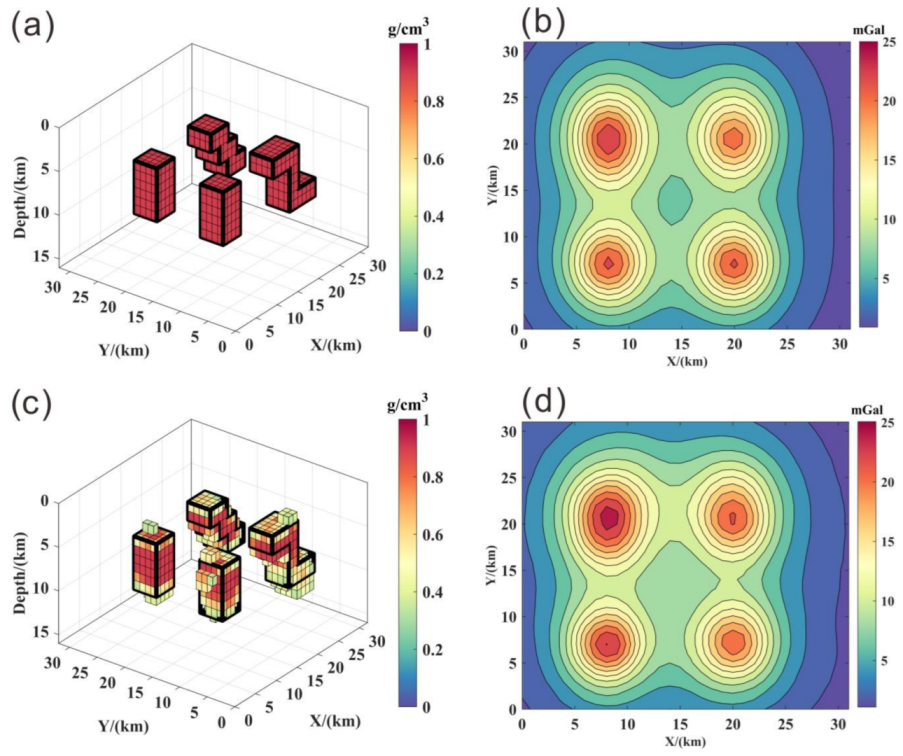
3.5. Inversion Results of the Synthetic Model Data

The gravity data corresponding to the synthetic model are input into the trained network, yielding inversion results for the model. To assess the effectiveness of the presented inversion method, we constructed a model consisting of horizontally adjacent superimposed prisms (Figure 6a). This model consisted of two parallel individual prisms with different depths, and the associated gravity anomaly is shown in Figure 6b. The deep learning density inversion method established in this study was used to invert the gravity data as presented in Figure 6b. Consequently, the 3D density distribution results were obtained, as shown in Figure 6c. Moreover, the 3D physical property inversion results exclusively showed the density value distribution greater than 0.5 g/cm³. From Figure 6c, it becomes evident that the proposed method can effectively reconstruct the 3D spatial structure of the prism. The results align at the top of the prisms, although the inversion outcomes at the prism bottom appear somewhat indistinct. The gravity data anomaly resulting from the forward calculation of the 3D physical property inversion results is shown in Figure 6d. Upon comparison with the theoretical gravity data anomalies (Figure 6b), it becomes evident that the data-driven inversion method effectively fits the density parameter inversion. These results show that the loss function, incorporating physical constraints, steers the network training process, yielding inversion results that align closely with the gravity forward theory and exhibit strong fitting.

To enhance the clarity of the correspondence between the density values in the inversion results and those of the density value of the actual model, cross-sectional slices passing through the model’s center were selected for the display of the 3D inversion results (Figure 7). Within the middle and upper sections of the model, the physical property inversion results exhibited a higher level of accuracy, closely aligning with the density parameters within the model. In contrast, in the deeper sections of the model, the inversion results displayed some divergence. However, the overall inversion results can effectively reflect the model’s spatial position and physical parameters.

This study established an inclined step model to assess the effectiveness of a gravity inversion method under complex geological conditions. Figure 8a shows a spatial location map of the model comprising two inclined steps with the resulting gravity anomaly shown in Figure 8b. The deep learning inversion method, as adopted in this study, was used to generate 3D density distribution results (Figure 8c). The inversion results show that the deep learning method can effectively determine the spatial position of the inclined step. Meanwhile, the density distribution results can effectively determine the inclination information of the inclined step. This indicates that the proposed method has a good application effect in the inversion of inclined geological structures. By performing forward calculation based on the inverted performance density distribution, the calculated gravity anomalies in Figure 8d were obtained. These anomalies were in good agreement with the theoretical gravity anomalies, providing validation of the accuracy of the inversion results.

Observing the slices of the inversion results, it becomes evident that the inverted density values obtained through the proposed method closely match the actual density value of 1 g/cm³ in the shallow position of the model. While some divergence is present in the deeper positions, densities greater than 0.5 g/cm³ effectively contribute to determine the model’s spatial position (Figure 9).

To assess and test the applicability of the proposed method in detecting anomalies caused by vertically superimposed prisms, a model as shown in Figure 10a was established to evaluate the effectiveness of the proposed method. The inversion results (Figure 10c) reveal that the deep learning-based inversion method adeptly reconstructed the 3D structure of two prisms with different depths, although the inversion accuracy for the deeper prisms was somewhat diminished.

To prove the inversion effect of the proposed method in the case of complex models, a complex model composed of multiple models of different types was designed in this study, as shown in Figure 11a. The model consisted of two prisms, an inclined step, and a Z-shaped model. The inversion result is shown in Figure 11c. Note the solid black lines representing the boundary of the model in the figure. It can be seen from the results that although the complexity of the model increased, the method still had a good inversion effect and a good fitting degree on the model boundary. The inversion results were good on the top and bottom of the Z-shaped model and the whole of the inclined steps. Figure 11b,d show the forward data of the actual model and the prediction model, respectively, showing a high fitting accuracy of the inversion results.

To quantitatively analyze the model inversion results, here we used two analytical metrics, model fitting and data fitting, to evaluate the model inversion errors. Model fitting ($E_m$) and data fitting ($E_d$) were used to measure the error between the inversion model and the real model and the error between the corresponding anomaly, respectively, as follows:

$$E_m={‖m-\widehat{m}‖}_{L2}^2$$

(17)

$$E_d={‖d-\widehat{d}‖}_{L2}^2$$

(18)

From

Table 1. Error statistics of inversion results from models I–IV, the horizontal adjacent superimposed prisms, the inclined step model, vertically superimposed prisms, and the complex model, respectively.

Model	${\mathit{E}}_{\mathit{m}}$	${\mathit{E}}_{\mathit{d}}$
Model I	11.0988	21.0992
Model I (without data fitting)	11.0823	60.2477
Model II	13.8248	20.9244
Model II (without data fitting)	14.3762	73.0496
Model III	14.9442	25.7893
Model III (without data fitting)	15.0122	69.4803
Model IV	13.9615	17.7656
Model IV (without data fitting)	13.7121	67.6317

, it is revealed that the method proposed in this paper has obvious advantages in data fitting, by means of error statistics of inversion results between the method proposed in this paper and the deep learning inversion method without the data fitting term.

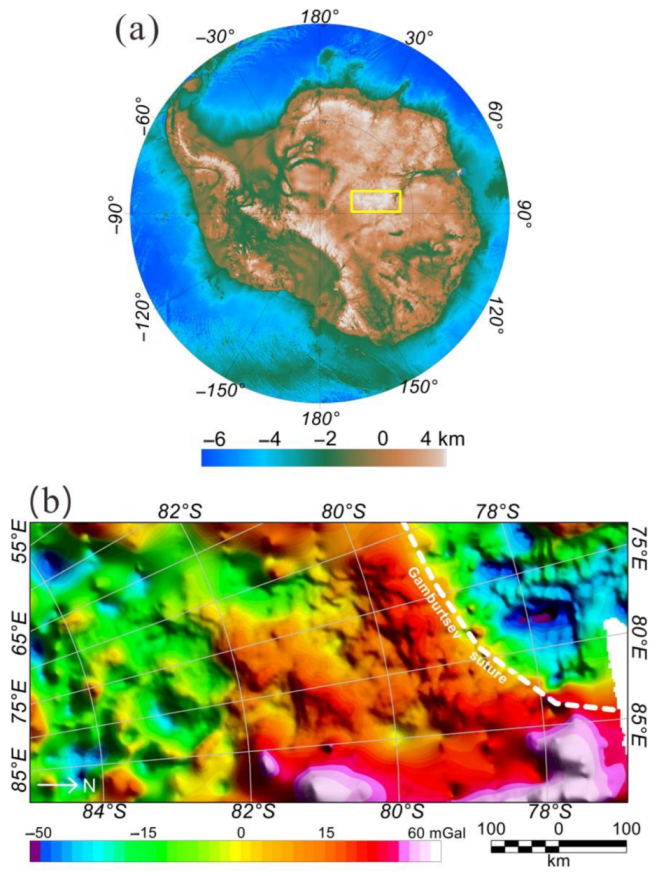
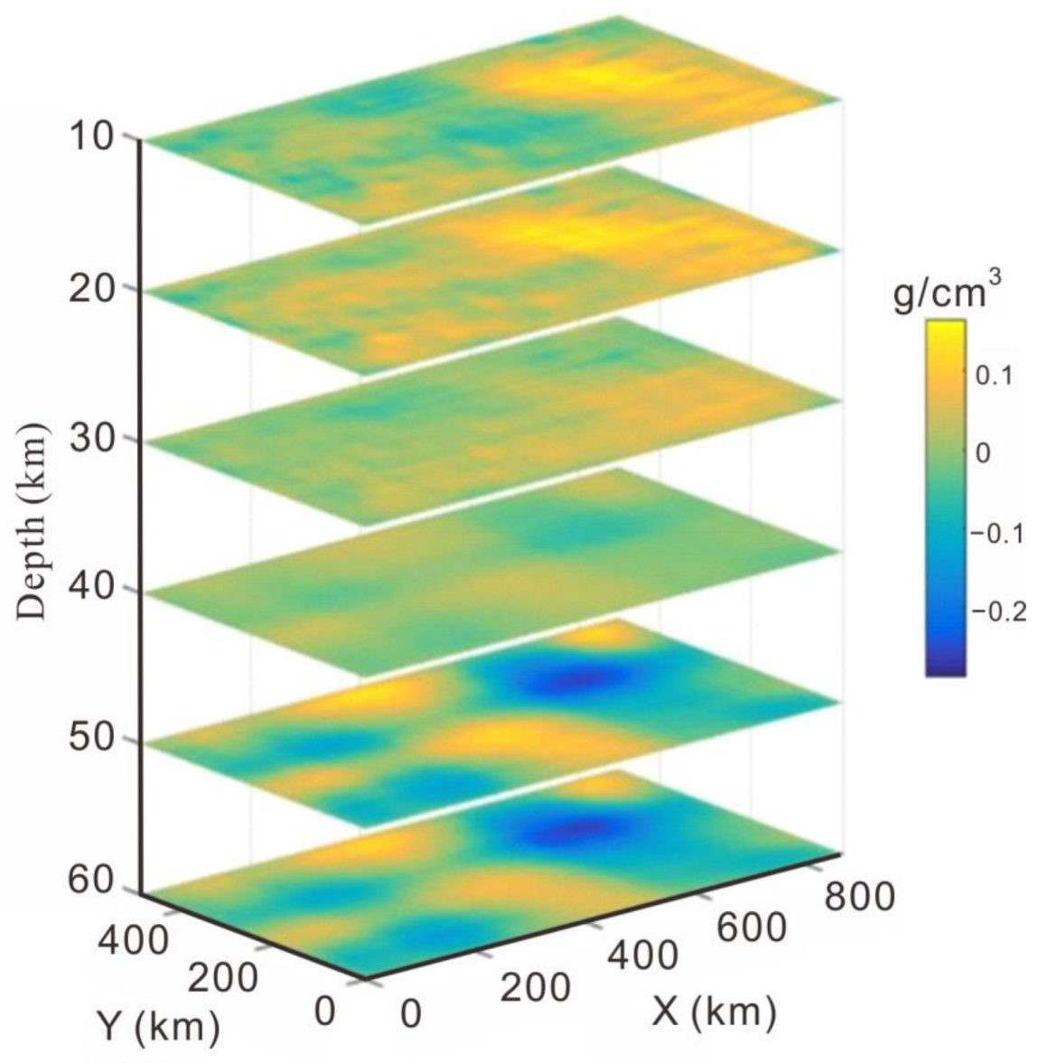
4. Application in East Antarctica

To prove its effectiveness in a real case, we applied this improved inversion method to the gravity data collected over the Gamburtsev Subglacial Mountains (GSM) in East Antarctica, which are entirely concealed beneath the East Antarctic Ice Sheet. An integrated airborne geophysical exploration of the GSM was carried out as part of the Antarctica’s Gamburtsev Province Project (AGAP) during the Fourth International Polar Year 2008/2009 [31]. It was the first detailed international collaborative aerogeophysical exploration effort in the GSM [32]. Figure 12 provides the schematic map and the isostatic residual gravity anomaly map of the GSM [32,33,34].

Due to the hostile environment and thick ice sheet in the interior of East Antarctica, airborne geophysical methods became one effective means to explore the GSM. The subglacial bed map revealed by the airborne radar data shows the enigmatic intraplate mountain range [31]. The average altitude of the subglacial topography was about 1.4 km, and the maximum height reached about 3.4 km [35]. The mountain ranges were underlain by over 58 km thick crust and 200 km thick lithosphere [33,36]. The GSM have been a key site for the evolution of the East Antarctic Precambrian cratonic lithosphere. However, little is known about the deep crustal structure and tectonic history of the huge mountains. By utilizing airborne geophysical data, a tectonic model was proposed, suggesting that the uplift of the GSM was triggered by the Permian and Cretaceous East Antarctic rift system, as a result of erosional unloading and heating of the crustal root [33]. The old root may undergo a reactivation process during later Permian and Cretaceous rifting, possibly formed during the Proterozoic assembly of East Antarctica and preserved in the old orogens. The mountains, whose surface was lifted in the early GSM formation, were severely eroded, while the lower crust was inferred to be well preserved. Based on the comprehensive analysis of the determined crustal geometry and geological context of East Antarctica, a new evolutionary framework is proposed by Wu et al. (2023), suggesting that the GSM have been a part of the Pan-African advancing accretionary orogen superimposed on the Precambrian basement [32]. The uplift mechanism of the GSM is still controversial, but the presence of a dense lower crustal root beneath the GSM is noticed. The Te grid calculated by Ferraccioli et al. (2011) reveals that the thick and dense Precambrian crust that underlies the central and northern portions of the GSM [33]. These high Te values are routinely associated with unreworked Precambrian cratonic regions worldwide.

Figure 12. (a) Schematic map showing the application of the improved gravity inversion method based on deep learning over the GSM of East Antarctica, using the base map from BEDMAP2 [37]. The study area is highlighted in the yellow rectangle. (b) Map depicting the isostatic residual gravity anomaly [32,33,34].

Figure 12. (a) Schematic map showing the application of the improved gravity inversion method based on deep learning over the GSM of East Antarctica, using the base map from BEDMAP2 [37]. The study area is highlighted in the yellow rectangle. (b) Map depicting the isostatic residual gravity anomaly [32,33,34].

In depicting the 3D crustal density structures over the GSM, here we used the isostatic residual gravity to invert relative density. Using the deep learning U-net network model established with synthetic model data, we processed the isostatic residual gravity data derived from the GSM. The underground space of the GSM was uniformly divided into 123,200 prisms with grids of $88\times 50\times 28$. The horizontal and vertical spacings were 10 km and 2.5 km, respectively. The obtained 3D inversion results are shown in Figure 13. Within these results, the remarkable high-density region can be found at a slice of depth 50 km. To highlight the detailed high-density lower crust, we extracted the 3D density structures of the crustal root from depths of 38 km to 68 km and conducted a quantitative comparison with the previous researches. The 3D detailed density structures of the lower crust are presented in Figure 14. Figure 14a–f show the horizontal density slices of the crustal root. The distinct density boundaries between the northern and central GSM were possibly related to the density difference of the Gamburtsev Suture sandwiched between the Antarctica–Australia terrain and Antarctica–India terrain. Figure 14g–n display the vertical density structure slices of lower crust in Y direction and X direction, respectively, with the depth range of 38–68 km. The upper part of the high-density block in (g) and (h) has a larger range than the lower part, like an inverted triangle, having a similar pattern to the two models in (r) and (s). To exhibit the high-density structures intuitively and visually, 3D voxels were used to display the dense blocks with different density ranges. Figure 14o–q show the dense blocks with density ranges of 0.02~0.16 $\mathrm{g}/{\mathrm{c}\mathrm{m}}^3$, 0.04~0.16 $\mathrm{g}/{\mathrm{c}\mathrm{m}}^3$, and 0.06~0.16 $\mathrm{g}/{\mathrm{c}\mathrm{m}}^3$. Figure 14r,s show the 2D geological and geophysical models proposed by Ferraccioli et al. (2011) and Wu et al. (2023) [32,33]. The 2D models were established along the profile $a–a^{\prime }$ shown in Figure 14a. Subsequently, a quantitative evaluation was conducted by determining the spatial locations of the high-density blocks in the lower crust displayed by 3D voxels within different density ranges and contrasting the results with the previous research.

Table 2. Contrast of the spatial locations of the high-density lower crust between our results from the improved inversion method based on U-net network and the previous 2D models.

Comparing Objects	Density Ranges in g/cm3	X-Axis Ranges in km	Depth Ranges in km
This study	0.02–0.16	245–560	40–68
	0.04–0.16	260–550	40–67
	0.06–0.16	300–520	40–60
Ferraccioli et al., 2011 [33]	-	250–680	46–58
Wu et al., 2023 [32]	-	245–670	40–58

shows the contrast of the spatial locations of the high-density lower crust between our results from the improved inversion method based on U-net network and the previous 2D models. The horizontal ranges in X direction were 245–560 km, 260–550 km, and 300–520 km, and the corresponding densities were 0.02–0.16 $\mathrm{g}/{\mathrm{c}\mathrm{m}}^3$, 0.04~0.16 $\mathrm{g}/{\mathrm{c}\mathrm{m}}^3$, and 0.06~0.16 $\mathrm{g}/{\mathrm{c}\mathrm{m}}^3$, respectively. Meanwhile, the horizontal ranges obtained from the 2D models of Ferraccioli et al. (2011) and Wu et al. (2023) [32,33] were 250–680 km and 245–670 km, respectively. Our results in the X direction were basically covered by horizontal ranges suggested by the previous studies. Vertically, the depth values were 40–68 km, 40–67 km, and 40–60 km obtained from the three different density ranges, which were close to the depth ranges of 46–58 km and 40–58 km achieved from the previous studies. Based on this contrast, it becomes evident that selecting the density range between 0.06 and 0.16 $\mathrm{g}/{\mathrm{c}\mathrm{m}}^3$ may prove advantageous in highlighting the high-density lower crust in depth.

These lower bodies potentially signify magmatic underplating associated with back-arc basin formation, triggered by the subduction of oceanic lithosphere located between Australo-Antarctica and Indo-Antarctica before their collision. The remarkable density boundary emerges between the northern and central sectors of the GSM at depths of 50 km and 60 km. This boundary might correspond to the Gamburtsev Suture, which separates the Archaean Ruker province and the Proterozoic Gamburtsev province [33]. The low-density region within the Lambert Terrain is consistent with the inferred forearc basin and accreted arc region [32]. The high-density region beneath the central and northern GSM domain shares a similar size to the dense root proposed by Ferraccioli et al. (2011) [33]. Notably, the dense region at the central GSM is disconnected and twists southward, possibly linked with a large fault system relevantly like the strike-slip fault with traits of a trailing contractional imbrication fan proposed by Wu et al. (2023) based on the aeromagnetic anomaly [32]. The results obtained from the 3D inversion of crustal density are consistent with the previous studies, which further verifies the effectiveness of this improved gravity inversion method.

5. Discussion

According to the outcomes of synthetic model testing and real data application in East Antarctica, it can be inferred that the method proposed in this study yields favorable 3D density structures. This method not only successfully restores and reconstructs the synthetic model but also demonstrates a satisfactory concordance between the inversion results of the field data and the synthetic model data. In terms of data fitting, the contrast results reveal that the method proposed in this paper has obvious advantages in data fit-ting, by means of error statistics of inversion results between the method proposed in this paper and the deep learning inversion method without the data fitting term. The method proposed in this study incorporates the data fitting term to constrain the inversion process, thereby obtaining outcomes closer to the real situation and enhancing the accuracy of the inversion results.

The method presented in this study has the potential to enhance the outcomes of 3D density inversion for gravity data. However, it is important to acknowledge that certain challenges persist, such as the requirement for human intervention in parameter verification during the inversion process, which relies on empirical approaches. The quantification and objectivity of inversion need to be improved. Meanwhile, there is a pressing need to enhance the precision of inversion outcomes for vertically superimposed objects, a limitation inherent to the current method and a formidable challenge in the field of gravity inversion. Future research endeavors will focus on incorporating additional constraints and priori information to strengthen the stability and robustness of 3D gravity inversion.

6. Conclusions

This study presents an improved 3D density inversion method for gravity data, utilizing the U-net network and optimizing the existing loss function. To bolster inversion convergence and constrain outcomes, a physical constraint term has been integrated into this approach, quantifying the level of data fitting between the predicted and the actual gravity anomalies. To enhance both the sample set generalization and the inversion accuracy, extensive training and test sets are generated by the random walk method aligned with gravity forward theory. This methodology’s effectiveness is demonstrated through evaluations of both a single model and a complex combination model. Through an analysis of synthetic data, this improved inversion method demonstrates favorable outcomes in the reconstruction of relative density. Applying this method to measured airborne gravity data collected over the GSM of East Antarctica yields a comprehensive 3D crustal density model. Notably, high-density bodies are identified in the lower crust beneath the central GSM, which may reflect magmatic underplating associated with back-arc basin formation. Moreover, the distinct density boundary between the northern and central GSM at depths ranging from 50 to 60 km may reflect the Gamburtsev Suture, which separates the Archaean Ruker province from the Proterozoic Gamburtsev province. Our findings provide a novel perspective for the study of crustal structure and geological evolution in East Antarctica.

References

1. Li, Y.; Oldenburg, D.W. 3-D inversion of gravity data. Geophysics 1998, 63, 109–119. [Google Scholar] [CrossRef]
2. Nabighian, M.N.; Ander, M.E.; Grauch, V.J.S.; Hansen, R.O.; LaFehr, T.R.; Li, Y.; Pearson, W.C.; Peirce, J.W.; Phillips, J.D.; Ruder, M.E. Historical development of the gravity method in exploration. Geophysics 2005, 70, 63ND–89ND. [Google Scholar] [CrossRef]
3. Oldenburg, D.W. The Inversion and interpretation of gravity anomalies. Geophysics 1974, 39, 526–536. [Google Scholar] [CrossRef]
4. Silva, J.B.C.; Costa, D.C.L.; Barbosa, V.C.F. Gravity inversion of basement relief and estimation of density contrast variation with depth. Geophysics 2006, 71, J51–J58. [Google Scholar] [CrossRef]
5. Tikhonov, A.N.; Goncharsky, A.V.; Stepanov, V.V.; Yagola, A.G. Numerical methods for the approximate solution of ill-posed problems on compact sets. In Numerical Methods for the Solution of Ill-Posed Problems; Springer: Dordrecht, The Netherlands, 1995; pp. 65–79. [Google Scholar] [CrossRef]
6. Li, Y.; Oldenburg, D.W. 3-D inversion of magnetic data. Geophysics 1996, 61, 394–408. [Google Scholar] [CrossRef]
7. Last, B.J. Compact gravity inversion. Geophysics 2012, 48, 713–721. [Google Scholar] [CrossRef]
8. Portniaguine, O.; Zhdanov, M.S. Focusing geophysical inversion images. Geophysics 1999, 64, 874–887. [Google Scholar] [CrossRef]
9. Zhang, Y.; Wu, Y.; Yan, J.; Wang, H.; Qiu, Y. 3D inversion of full gravity gradient tensor data in spherical coordinate system using local north-oriented frame. Earth Planets Space 2018, 70, 58. [Google Scholar] [CrossRef]
10. Portniaguine, O.; Zhdanov, M.S. 3-D magnetic inversion with data compression and image focusing. Geophysics 2002, 67, 1532–1541. [Google Scholar] [CrossRef]
11. Li, Y.; Oldenburg, D.W. Fast inversion of large-scale magnetic data using wavelet transforms and a logarithmic barrier method. Geophys. J. Int. 2003, 152, 251–265. [Google Scholar] [CrossRef]
12. Foks, N.L.; Krahenbuhl, R.; Li, Y. Adaptive sampling of potential-field data: A direct approach to compressive inversion. Geophysics 2014, 79, IM1–IM9. [Google Scholar] [CrossRef]
13. Zhang, L.; Zhang, G.; Liu, Y.; Fan, Z. Deep Learning for 3-D Inversion of Gravity Data. IEEE Trans. Geosci. Remote Sens. 2022, 60, 5905918. [Google Scholar] [CrossRef]
14. Guo, R.; Yao, H.M.; Li, M.; Ng, M.K.P.; Abubakar, A. Joint Inversion of Audio-Magnetotelluric and Seismic Travel Time Data With Deep Learning Constraint. IEEE Trans. Geosci. Remote Sens. 2020, 59, 7982–7995. [Google Scholar] [CrossRef]
15. Kim, Y.; Nakata, N. Geophysical inversion versus machine learning in inverse problems. Lead. Edge 2018, 37, 894–901. [Google Scholar] [CrossRef]
16. Mousavi, S.M.; Beroza, G.C. Deep-learning seismology. Science 2022, 377, eabm4470. [Google Scholar] [CrossRef]
17. Li, J.; Liu, Y.; Yin, C.; Ren, X.; Su, Y. Fast imaging of time-domain airborne EM data using deep learning technology. Geophysics 2020, 85, E163–E170. [Google Scholar] [CrossRef]
18. Puzyrev, V. Deep learning electromagnetic inversion with convolutional neural networks. Geophys. J. Int. 2019, 218, 817–832. [Google Scholar] [CrossRef]
19. Qi, S.; Wang, Y.; Li, Y.; Wu, X.; Ren, Q.; Ren, Y. Two-Dimensional Electromagnetic Solver Based on Deep Learning Technique. IEEE J. Multiscale Multiphysics Comput. Tech. 2020, 5, 83–88. [Google Scholar] [CrossRef]
20. Guo, J.; Li, Y.; Jessell, M.W.; Giraud, J.; Li, C.; Wu, L.; Li, F.; Liu, S. 3D geological structure inversion from Noddy-generated magnetic data using deep learning methods. Comput. Geosci. 2021, 149, 104701. [Google Scholar] [CrossRef]
21. Khan, A.; Ghorbanian, V.; Lowther, D. Deep Learning for Magnetic Field Estimation. IEEE Trans. Magn. 2019, 55, 7202304. [Google Scholar] [CrossRef]
22. Pollok, S.; Bjørk, R.; Jørgensen, P.S. Inverse Design of Magnetic Fields Using Deep Learning. IEEE Trans. Magn. 2021, 57, 2101604. [Google Scholar] [CrossRef]
23. Yang, Q.; Hu, X.; Liu, S.; Jie, Q.; Wang, H.; Chen, Q. 3-D Gravity Inversion Based on Deep Convolution Neural Networks. IEEE Geosci. Remote Sens. Lett. 2022, 19, 3001305. [Google Scholar] [CrossRef]
24. Zhang, S.; Yin, C.; Cao, X.; Sun, S.; Liu, Y.; Ren, X. DecNet: Decomposition network for 3D gravity inversion. Geophysics 2022, 87, G103–G114. [Google Scholar] [CrossRef]
25. Huang, R.; Liu, S.; Qi, R.; Zhang, Y. Deep Learning 3D Sparse Inversion of Gravity Data. J. Geophys. Res. Solid Earth 2021, 126, e2021JB022476. [Google Scholar] [CrossRef]
26. Wang, Y.-F.; Zhang, Y.-J.; Fu, L.-H.; Li, H.-W. Three-dimensional gravity inversion based on 3D U-Net++. Appl. Geophys. 2021, 18, 451–460. [Google Scholar] [CrossRef]
27. Chen, Z.; Chen, Z. The Identification of Impact Craters from GRAIL-Acquired Gravity Data by U-Net Architecture. Remote Sens. 2022, 14, 2783. [Google Scholar] [CrossRef]
28. Boulanger, O.; Chouteau, M. Constraints in 3D gravity inversion. Geophys. Prospect. 2001, 49, 265–280. [Google Scholar] [CrossRef]
29. Li, X.; Chouteau, M. Three-Dimensional Gravity Modeling In All Space. Surv. Geophys. 1998, 19, 339–368. [Google Scholar] [CrossRef]
30. Nagy, D.; Papp, G.; Benedek, J. The gravitational potential and its derivatives for the prism. J. Geod. 2000, 74, 552–560. [Google Scholar] [CrossRef]
31. Bell, R.E.; Ferraccioli, F.; Creyts, T.T.; Braaten, D.; Corr, H.; Das, I.; Damaske, D.; Frearson, N.; Jordan, T.; Rose, K.; et al. Widespread Persistent Thickening of the East Antarctic Ice Sheet by Freezing from the Base. Science 2011, 331, 1592–1595. [Google Scholar] [CrossRef] [PubMed]
32. Wu, G.; Ferraccioli, F.; Zhou, W.; Yuan, Y.; Gao, J.; Tian, G. Tectonic Implications for the Gamburtsev Subglacial Mountains, East Antarctica, from Airborne Gravity and Magnetic Data. Remote Sens. 2023, 15, 306. [Google Scholar] [CrossRef]
33. Ferraccioli, F.; Finn, C.A.; Jordan, T.A.; Bell, R.E.; Anderson, L.M.; Damaske, D. East Antarctic rifting triggers uplift of the Gamburtsev Mountains. Nature 2011, 479, 388–392. [Google Scholar] [CrossRef] [PubMed]
34. Wu, G.; Tian, G.; Bangbing, W.; Ferraccioli, F.; Seddon, S.; Finn, C.; Bell, R. Crustal structure of the Gamburtsev Province, East Antarctica, from airborne geophysics. In Proceedings of the 2017 SEG International Exposition and Annual Meeting, Houston, TX, USA, 24–29 September 2017. [Google Scholar]
35. Bo, S.; Siegert, M.J.; Mudd, S.M.; Sugden, D.; Fujita, S.; Xiangbin, C.; Yunyun, J.; Xueyuan, T.; Yuansheng, L. The Gamburtsev mountains and the origin and early evolution of the Antarctic Ice Sheet. Nature 2009, 459, 690–693. [Google Scholar] [CrossRef] [PubMed]
36. An, M.; Wiens, D.A.; Zhao, Y.; Feng, M.; Nyblade, A.A.; Kanao, M.; Li, Y.; Maggi, A.; Lévêque, J.-J. S-velocity model and inferred Moho topography beneath the Antarctic Plate from Rayleigh waves. J. Geophys. Res. Solid Earth 2015, 120, 359–383. [Google Scholar] [CrossRef]
37. Fretwell, P.; Pritchard, H.D.; Vaughan, D.G.; Bamber, J.L.; Barrand, N.E.; Bell, R.; Bianchi, C.; Bingham, R.G.; Blankenship, D.D.; Casassa, G. Bedmap2: Improved ice bed, surface and thickness datasets for Antarctica. Cryosphere Discuss. 2013, 7, 375–393. [Google Scholar] [CrossRef]
Figure 1. Schematic diagram of underground space.
Remotesensing 15 04933 g001
Figure 2. Schematic diagram of gravity data inversion network structure.
Remotesensing 15 04933 g002
Figure 3. The expression and pattern of the Tanh function.
Remotesensing 15 04933 g003
Figure 4. Schematic diagram of random walk generation model: (a) The model of random walk for 10 steps. (b) The model of random walk for 30 steps.
Remotesensing 15 04933 g004
Figure 5. Schematic diagram of density model.
Remotesensing 15 04933 g005
Figure 6. Inversion results of the model with horizontal adjacent superimposed prisms: (a,b) The model distribution and its gravity anomaly. (c,d) The inversion result and its anomaly.
Remotesensing 15 04933 g006
Figure 7. Inversion slice results of the model with horizontal adjacent superimposed prisms: (a) The model distribution. (b) The inversion result.
Remotesensing 15 04933 g007
Figure 8. Inversion results of the inclined step model: (a,b) The model distribution and its corresponding gravity anomaly. (c,d) The inversion result and its associated anomaly.
Remotesensing 15 04933 g008
Figure 9. Inversion slice results of the inclined step model: (a) The model distribution. (b) The inversion result.
Remotesensing 15 04933 g009
Figure 10. Inversion results of the model with vertically superimposed prisms: (a,b) The model distribution and its corresponding gravity anomaly. (c,d) The inversion result and its associated anomaly.
Remotesensing 15 04933 g010
Figure 11. Inversion results of the complex model: (a,b) The model distribution and its gravity anomaly. (c,d) The inversion result and its anomaly.
Remotesensing 15 04933 g011
Figure 13. Horizontal slices of crustal density inversed from the GSM gravity anomaly.
Remotesensing 15 04933 g013
Figure 14. The 3D density structures of the GSM lower crust and comparison with the previous studies. The detailed horizontal density structures of the lower crust are presented in (af) with 6 km vertical spacing in the Z direction. The white line a a represents the profile location of the 2D model in (r,s). (gj) and (kn) show the vertical density structure slices of lower crust in the Y direction and the X direction, respectively. The depth range is 38–68 km. (oq) show the high-density blocks in the lower crust with the residual density ranges of 0.02–0.16 g / c m 3 , 0.04–0.16 g / c m 3 , and 0.06–0.16 g / c m 3 , respectively. (r,s) show the 2D geological and geophysical models unveiled by previous studies [32,33]. Note the yellow polygons highlighting the high-density lower crust.
Remotesensing 15 04933 g014