Article

A Downscaling Methodology for Extracting Photovoltaic Plants with Remote Sensing Data: From Feature Optimized Random Forest to Improved HRNet

1
Aerospace Information Research Institute, Chinese Academy of Sciences, Beijing 100094, China
2
School of Electronic, Electrical and Communication Engineering, University of Chinese Academy of Sciences, Beijing 100049, China
3
University of Chinese Academy of Sciences, Beijing 100049, China
*
Author to whom correspondence should be addressed.
Remote Sens. 2023, 15(20), 4931; https://doi.org/10.3390/rs15204931
Submission received: 20 August 2023 / Revised: 9 October 2023 / Accepted: 10 October 2023 / Published: 12 October 2023
(This article belongs to the Special Issue Remote Sensing of Renewable Energy)

Abstract

:
Present approaches in PV (Photovoltaic) detection are known to be scalable to a larger area using machine learning classification and have improved accuracy on a regional scale with deep learning diagnostics. However, it may cause false detection, time, and cost-consuming when regional deep learning models are directly scaled to a larger area, particularly in large-scale, highly urbanized areas. Thus, a novel two-step downscaling methodology integrating machine learning broad spatial partitioning (step-1) and detailed deep learning diagnostics (step-2) is designed and applied in highly urbanized Jiangsu Province, China. In the first step, this methodology selects suitable feature combinations using the recursive feature elimination with distance correlation coefficient (RFEDCC) strategy for the random forest (RF), considering not only feature importance but also feature independence. The results from RF (overall accuracy = 95.52%, Kappa = 0.91) indicate clear boundaries and little noise. Furthermore, the post-processing of noise removal with a morphological opening operation for the extraction result of RF is necessary for the purpose that less high-resolution remote sensing tiles should be applied in the second step. In the second step, tiles intersecting with the results of the first step are selected from a vast collection of Google Earth tiles, reducing the computational complexity of the next step in deep learning. Then, the improved HRNet with high performance on the test data set (Intersection over Union around 94.08%) is used to extract PV plants from the selected tiles, and the results are mapped. In general, for Jiangsu province, the detection rate of the previous PV database is higher than 92%, and this methodology reduces false detection noise and time consumption (around 95%) compared with a direct deep learning methodology.

1. Introduction

The production of energy from traditional energy sources (i.e., coal, fossil, and natural gas) is responsible for 87% of global greenhouse gas emissions. Therefore, bringing emissions down toward net zero will be one of the world’s biggest challenges in the years ahead [1]. Solar energy is one way to ensure a cleaner, greener, and more sustainable future [2,3,4]. In China, the cumulative solar PV capacity has been developing rapidly for achieving the goal of “Carbon peaking and carbon neutrality”. For example, by the first half year of 2021, China’s cumulative solar PV capacity has grown to 267.086 GW with an increment of 13.011 GW (approximately 5% per half year) [5]. Besides the quantity of cumulative solar PV capacity, it is necessary to understand the distribution of existing PV plants for further quantifying regional solar power generation potentials [6]. The development of remote sensing technology in terms of its temporal, spatial, and spectral resolution, combined with advanced artificial intelligence technology, is effectively used for the detection of PV plants [7,8,9].
In application, machine learning-based PV classification is scalable to a larger area and shows ability in the continuity of PV condition monitoring using moderate-resolution remote sensing imagery (e.g., Sentinel1 Sentinel2 and Landsat [10,11,12]). It is cost-effective in terms of using publicly available data and requiring fewer training samples [13]. For example, machine learning approaches such as random forest (RF) and support vector machine (SVM) are used to detect PV plants in coastal and inland [14], in arid regions of five provinces in northwestern China [12,15], and in the northern part of the Netherlands [16]. However, the accuracy is limited by the moderate-resolution remote sensing imagery itself (Intersection over Union approximately (IoU) around 70~80% [16]) due to the so-called “different objects with the same spectrum” [17]. Besides, machine learning approaches require more features beyond what a single high-resolution remote sensing platform can supply, and for improving the PV categorizing accuracy, feature selection must be performed for consuming useful information [18]. Contrarily, deep learning-based PV diagnostics are more suitable for small-scale fine PV detection using only visible bands [19,20,21,22] and/or multispectral data [23] from high-resolution remote sensing imagery. It alleviates the issue of PV false detection related to “different objects with the same spectrum” and achieves a higher accuracy (IoU around 80~90% [24]). However, for large-scale research, this approach could be time-consuming and expensive in high-resolution remote sensing imagery purchasing [25].
Some hierarchical methods are designed to bypass the issue of time and cost-consuming. For example, aerial images and a cascade methodology including random forest and convolutional neural networks (CNNs) are used to extract PV plants in the US city of Fresno, California [26]. Kruitwagen et al. [27] create a global PV database using a two-step methodology including “global search” and “filtering”. First, U-Net [28] is used to identify the possible PV areas with SPOT 6/7 and Sentinel-2 data. Second, the LSTM model and hand verification are used to eliminate the false detection of PV plants further. Although the methods reach high accuracy, the large-scale aerial images and SPOT 6/7 data are not freely available in China. Yu et al. [29] propose a hierarchical “Deepsolar” structure for extracting PV panels in the United States. This method uses Inception-v3 [30] to classify remote sensing images with solar panels and then employs a semi-supervised approach to extract the PV panels. Ge et al. [31] extract possible PV areas from moderate-resolution remote sensing imagery (spatial resolution: 16 m, GaoFen-6) as candidate regions for further semantic segmentation using high-resolution remote sensing imagery (spatial resolution: 2 m, GaoFen-1). The IoU is improved to 90.6% by integrating PV detection advantages from both moderate-resolution and high-resolution remote sensing imagery. This approach is known to be efficient in less urbanized northwest China; however, it has limited accuracy (or high false detection) in our experiments in Eastern China, which is highly urbanized with complex land cover types [31]. This is because less missed or false detection in the first step of deep learning-based PV identification occurs over less urbanized northwest China due to regional homogeneous land cover types. However, more missed or false detection occurs in highly urbanized areas with the first step of learning deep learning-based PV identification. Besides, the influenced image tile has a pixel size (an area) of 512*512 (5122 × 162 m2), and as a result, the amount of consequent noise and missed PV plants surge in highly urbanized areas.
To complement large-scale PV detection over highly urbanized areas, a two-step downscaling machine learning and deep learning PV extraction method is designed combing the advantages of multisource satellite data (see Section 2), particularly for reducing the possibilities of missed or false detection in the first step and improving the efficiency in the second step. Here, instead of defining the binary status (PV, non-PV) of each image tile (e.g., an area of 5122 × 162 m2) with deep learning models, a machine learning model (RF) is used to extract possible PV plants in pixel scale with moderate-resolution satellite imagery (spatial resolution: 10 m). Followed by morphological open operations to remove noise in the RF extraction results, high-resolution Google Earth images (spatial resolution: 0.54 m) are selected by intersecting with the obtained PV extraction results before deep learning-based semantic segmentation of high-resolution satellite imagery. Note that the term “downscaling” [32,33,34] is the collective term that originally came from methods used to regionalize information from global climate models and create fine spatial scale projections of climate change, which is similar to this stepwise hierarchy from machine learning broad spatial partitioning (coarse spatial scale from Sentinel, 10 m × 10 m) to detailed deep learning diagnostics (fine spatial scale from Google, 0.54 m × 0.54 m).
In the following, this paper explains the machine learning broad spatial partitioning (step-1) and the detailed deep learning diagnostics (step-2) method (see Section 2). Then, Jiangsu province is selected to demonstrate this two-step methodology (see Section 3). Model comparison and discussion (see Section 4) evaluate this two-step methodology before a concluding summary (see Section 5).

2. Materials and Methodology

For large-scale applications, satellite data have a significant cost advantage over other platforms (i.e., spaceborne, airborne, and ground-based). In this paper, moderate-resolution satellite data (visible-light imagery, spectral imagery, and synthetic aperture radar (SAR) imagery), Digital Elevation Model data (DEM), and high-resolution Google Earth images are obtained to support the detection of the PV plants associated with training and validation data from existing PV database. Besides, remote sensing spectral indices (normalized difference built-up index (NDBI) [35], normalized difference vegetation index (NDVI) [36], modified normalized difference water index (MNDWI) [37], built-up area index (BUAI) [38], NDPI [39], NDPI2 [39], NIR_ratio [40], SWIR1_ratio [40], SWIR2_ratio [40]), texture features [41] (tonal or gray-level variations in an image (more details see Appendix A, Table A1)), geographical characteristics (slope, aspect, and hillshade) are jointly calculated (see Table 1) for identifying solar PV plants. The downscaling methodology for identifying solar PV plants with satellite remote sensing data follows a stepwise hierarchy from machine learning broad spatial partitioning (see Section 2.1,Section 2.2,Section 2.3 and Section 2.4) to detailed deep learning diagnostics (see Section 2.5 and Section 2.6) as shown in the flowchart (see Figure 1).

2.1. Training and Validation Samples Selection

Machine learning broad spatial partitioning and detailed deep learning diagnostics require different training samples: (1) For machine learning, the first step is creating buffers on ground-based PV observation points and then generating training points randomly within the buffer. Note that using high-resolution satellite images to validate the generated training and validation points is necessary for manually removing fake training and testing points. (2) For deep learning, ground-based PV observations are used to derive image chips for further training deep learning models. The first step is drawing the boundaries of the PV panels as a shapefile format according to the ground-based PV observations and then generating image-ground truth chips. Within (without) the boundary, the pixel value is set as 1 (0), representing PV plants (non-PV plants).

2.2. Feature Construction and Selection

Remote sensing observations, spectral indices, texture features, and graphical characteristics are all used as candidate features for supporting separating solar PV plants from the background. For example, PV panels are mainly composed of several crystalline silicon wafers with strong absorption of crystalline silicon in the visible wavelength band, reducing the reflectance of PV panel pixels [42]. The texture characteristics are chosen because the layout of PV panels is usually arranged regularly in the form of arrays [14]. The spectral indices help partition non-PV regions by enhancing the characteristics of different land cover types, such as buildups, water, and vegetation [14].
However, such a large number of candidate features requires an optimized selection before the model training process. This is because a large number of features not only causes a dimensionality disaster but sometimes even leads to recognition performance degradation [43]. Thus, the recursive feature elimination with distance correlation coefficient (RFEDCC) is implemented following the three subsequent steps:
  • Step-1 Machine Learning-based Recursive Feature Elimination (RFE):
The machine learning model is trained using all candidate features, and the importance of each feature is ranked. The feature with the lowest importance ranking is removed until the number of features reaches the setting threshold T1. In the previous work [12,14,15,16], random forest is used to extract PV plants, and the number of features is less than 20. Therefore, we set T1 to 20, ensuring that the first-step selection results have a moderate number of features while still containing sufficient information for distinguishing PV plants.
  • Step-2 Distance Correlation Coefficient-based Feature Elimination:
Features with similar importance will be eliminated according to their dependency. The distance correlation coefficient, which is sensitive to both linear and non-linear relationships, is used to calculate the dependency/similarity between each of the two selected features from step-1. When similarity or correlation coefficients are greater than T2, the less important feature, according to the step-1 ranking list, will be removed. Note that T2 is not a constant value here but ranges from 0.5 to 1 with a stepwise iteration of 0.05 in step-3 cross-validation.
  • Step-3 Iteration Validation and Selection:
All eleven different feature combinations obtained from the stepwise iteration (T2 ranging from 0.5 to 1, step = 0.05) are applied to the machine learning prediction model for cross-validation. Features in combination with the highest prediction accuracy will be the final model inputs for machine learning broad spatial partitioning of PV detection.
Note that step-2 considers feature efficiency between each two features, and step-3 focuses on combined feature redundancy. Compared with the number of all candidate features, the final selected features not only greatly reduce the model inputting feature size but also alleviate inter-feature correlation and feature redundancy issues.

2.3. Machine Learning Models

For the first step of machine learning broad spatial partitioning, three models are compared in PV detection with moderate-resolution remote sensing imagery.
  • Random Forest (RF): RF is a commonly-used machine learning algorithm trade-marked by Leo Breiman and Adele Cutler, which combines the output of multiple decision trees to vote for a single result [44]. In this study, the number of decision trees is set to 71, and the Gini index is used to evaluate feature importance.
  • Gradient Boosting Decision Tree (GBDT): GBDT has strong robustness and interpretability, which uses a loss function to optimize the model in steps of shrinkage [45]. In this study, the number of decision trees and the shrinkage are set to 127 and 0.005, respectively. The least absolute deviation loss function is used.
  • Support Vector Machine (SVM): SVM constructs a hyper-plane to maximize the distance between different classes [46]. In this study, the linear kernel is used to reduce the computational effort, and the regularization coefficient in SVM is set to 1 to improve the generalization ability.
Google Earth Engine (GEE) is a remote sensing big data analysis platform based on Google’s cloud service infrastructure. Here, RF, GBDT, and SVM are available with the GEE platform as ee.Classifier. smileRandomForest(), ee.Classifier. smileGradientTreeBoost() and ee.Classifier. libsvm() function, respectively.

2.4. Noise Removal and Enhancement

After achieving the results of machine learning broad spatial partitioning, a further morphological opening operation [47] is required to filter out the noise. The circular kernel is first used to perform the erosion operation on the original image to filter out noise areas with a small number of pixels and then perform the dilation operation to recover the corrupted PV plant pixels. This is also available with the GEE platform.

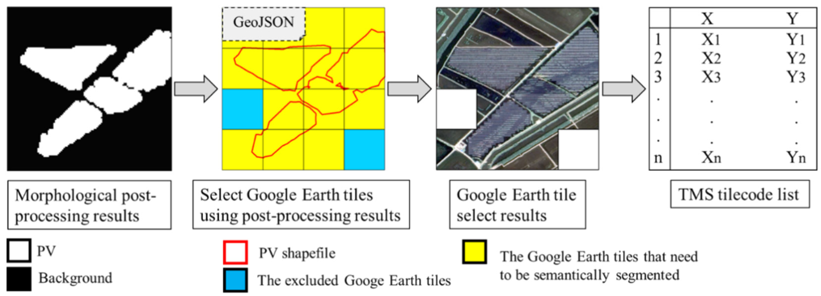
2.5. Tiles Selection associated with Google Earth Images

Following the morphological opening operation, the results of broad spatial partitioning with geographic latitudes and longitudes (lat, lon) panels are used for locating possible PV regions within high-resolution satellite imagery by selecting the corresponding Google Earth tiles (See Figure 2). In the process, spatial referencing systems should be unified to Tile Map Service (TMS) code to obtain tile indexes (xtile, ytile) with possible PV plants [48]:
x t i l e = R o u n d l o n + 180 ° 360 ° 2 z o o m
y t i l e = R o u n d ln tan l a t π / 180 + sec l a t π / 180 + π 2 π 2 z o o m 1
where zoom in this study is equal to 17, which is the tile level defined by Google Earth TMS. Round is a function to obtain the nearest integer.
Indeed, the results obtained from this step obtain a coarse extraction result (candidate Google Earth tiles), which is then input to the last step for refinement and mapping. This step is important because it eliminates a large number of invalid Google Earth tiles and contributes to accelerating the refinement procedure.

2.6. Deep Learning Diagnostics

The original HRNet is a general-purpose convolutional neural network for tasks like semantic segmentation, object detection, and image classification. The channel number of the top branch is selected as 32 in this study, HRNet-W32.
Semantic segmentation of this study uses HRNet-W32 as a backbone (see Figure 3a, from left to right) and starts from a high-resolution subnetwork, then gradually adding high-to-low resolution subnetworks in parallel. It maintains high-resolution features, providing four stages, four branches, and four resolutions. When the resolution is decreased to 1/4, 1/8, 1/16, and 1/32 of the original, the number of channels of the convolution layers is increased to 32, 64, 128, and 256. In application, the final four output features are mixed up to generate multi-scale semantic information. To fully follow its processing, readers are encouraged to view the original paper of HRNet [49].
Here, the sub-pixel convolution is used to reduce the information loss caused by bilinear upsampling of the final four output features (see Figure 3b. It is a commonly used method for image super-resolution tasks, which reconstructs a high-resolution version of an image from size H × W × C (H, W, and C mean height, width, and the number of channels, respectively) to size 2H × 2W × C/4 and maintains its content and details as much as possible. In this study, the feature maps output from the ②③④ branches of HRNet -W32 are applied to the sub-pixel convolution by sequentially fusing the previous layer output feature maps with feature pyramid networks (FPN) [50].
Experiments in this study run on an Ubuntu 16.04 operating system with NVIDIA TITAN-RTX (24 GB) graphics. The networks are implemented on the Pytorch 1.7.1 deep learning framework. For training, the network utilizes an SGD optimizer with an input image size of 256 × 256 and a batch size set to 16. The learning rate is adjusted throughout the training process using the exponential decay method, with an initial learning rate set to 0.0001, a decay exponent of 0.9, a weight decay of 0.0005, and a total number of epochs of 200. When the model’s loss does not decrease within ten epochs, the learning rate is adjusted to 1/10 of the current one. When the model goes through eight more epochs without decreasing, the training is stopped.
After training and testing the improved HRNet, Google Earth tiles selected from Section 2.5 will be applied to extract PV plants using the improved HRNet and mapping the extraction results.

2.7. Methodology and Result Evaluation

The concept of a confusion matrix for binary classification is used [51] to measure the efficiency of this downscaling methodology, where a model’s correct and incorrect classifications include true positive (TP, correct classification of PV plants), false positive (FP, incorrect classification of PV plants), true negative (TN, correct classification of non-PV), false negative (FN, incorrect classification of non-PV).
Evaluation Metrics for Machine Learning results: The Kappa coefficient, overall accuracy (OA), user accuracy (UA), and producer accuracy (PA) are used. The Kappa coefficient measures classification consistency. OA represents the overall accuracy. UA (PA) indicates the correct classification percentage for one predicted (ground truth) category.
O A = T P + T N T P + F P + F N + T N
K a p p a = O A P e 1 P e
w h e r e , p e = T P + F N T P + F P + F N + T N ( T N + F P ) T P + F P + F N + T N 2
U A p v = T P T P + F P
P A p v = T P T P + F N
U A n o n p v = T N T N + F N
P A n o n p v = T N T N + F P
Evaluation Metrics for Deep Learning results: To measure the accuracy of deep learning semantic segmentation methods in PV detection. Precision, Recall, F1-score, and intersection over union (IoU) are used.
P r e c i s i o n = T P T P + F P
R e c a l l = T P T P + F N
F 1 = 2 P r e c i s i o n R e c a l l P r e c i s i o n + R e c a l l
I o U = T P T P + F P + F N

3. Applications over Highly Urbanized Regions

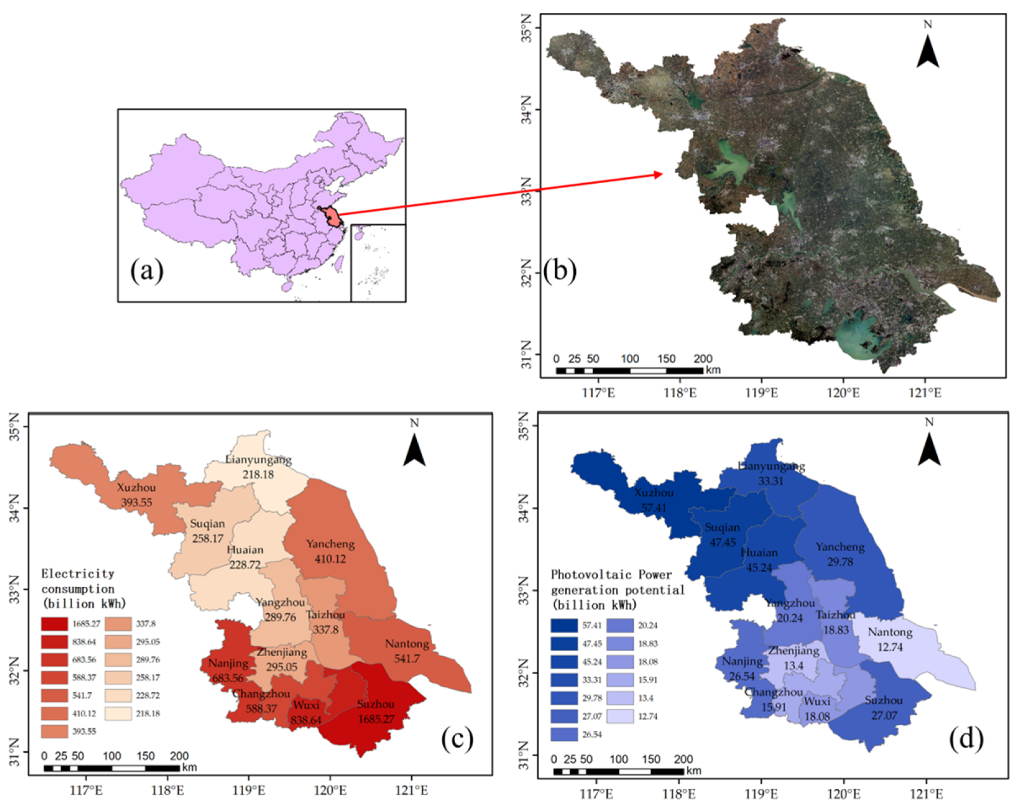
This downscaling methodology for extracting PV plants is applied in Jiangsu Province, China (107,200 km2, 30°45′~30°08′N, 116°21′~121°56′E) (see Figure 4b), which is highly urbanized and with a large demand for electricity (see Figure 4c, [52]). The total annual social electricity consumption of Jiangsu Province (Suzhou) exceeds 6500 billion kWh (even exceeds 1500 billion kWh) in 2021, while PV power generation is 195.32 billion kWh, although the local PV industry has been developed rapidly, e.g., a total of 17,646 MW by the first half year of 2021 [5]. The local theoretical solar energy resource of Jiangsu Province (Suzhou) is 366 billion kWh (even exceeding 27 billion kWh) per year (see Figure 4d); thus, the promising potential could be understood after diagnosing the present distribution of PV plants.
To diagnose the present distribution of PV plants, moderate-resolution satellite data (Sentinel-1, Sentinel-2), Digital Elevation Model data (DEM), and high-resolution Google Earth images are used for the first step of machine-learning broad spatial partitioning (see Section 2.1,Section 2.2,Section 2.3 and Section 2.4) and the second step of the detailed deep learning diagnostics (see Section 2.5 and Section 2.6). Present PV observations, including PV08 [53] (https://doi.org/10.5281/zenodo.5171712, last accessed on 5 May 2023), the Global Power Plant Database (GPPD) v1.3.0 [54] (https://datasets.wri.org/dataset/globalpowerplantdatabase, last accessed on 20 June 2023) and the PV plant database published by Kruitwagen et al. [27] (https://zenodo.org/record/5005868#.YzJjZXZByUl, last accessed on 20 June 2023), are used for training samples selection and result evaluation. Data used in this application are listed as follows:
  • Moderate-resolution satellite data: For the whole Jiangsu province, 80 tiles of Sentinel-1 Ground Range Detected SAR products (VV/VH) with a spatial resolution of 10 m × 10 m and 189 tiles of Sentinel2 L2A product with spatial resolutions of 10 m, 20 m, and 60 m are used for the first step machine learning broad spatial partitioning. Note that data from 04/01/2022 to 06/30/2022 with cloud coverage of less than 1% are selected for further GEE-based de-clouding, median filtering, mosaic, and cropping.
  • DEM: Shuttle Radar Topography Mission (SRTM) obtained from NASA [55] with a spatial resolution of 30 m is used.
  • High-resolution satellite data: Google Earth images (level 18, a mosaic dataset of Pleiades-1 and WorldView-3) with red, green, and blue bands and a spatial resolution of 0.54 m are acquired from the Google Earth API for the second step of the detailed deep learning diagnostics.
  • PV observations: The GPPD database was updated in June 2021. It records 1318 (115) PV power stations globally (in Jiangsu Province) and is used to derive training and testing samples for both machine-learning and deep-learning models. PV08 data set provides regional PV observations obtained from GaoFen-2 and BJ-2 satellites with a spatial resolution of 0.8 m, which will be used for adding additional training samples for enhancing the generalization of the improved HRNet methodology. Kruitwagen’s PV dataset provides 221 PV plants with confidence level A, which will be compared with results from this two-step methodology.
In general, together with spectral data (Sentinel-2: B2, B3, B4, B5, B6, B7, B8, B8A, B11, and B12), SAR data (Sentinel-1: VV and VH), remote sensing indices (NDBI, NDVI, MNDWI, BUAI, NDPI, NDPI2, NIR_ratio, SWIR1_ratio, and SWIR2_ratio), texture (the texture of Sentinel-2 data, Sentinel-1 data, NDBI, NDVI, MNDWI, and BUAI), DEM (Elevation), and geographical characteristics (Slope, Aspect, and Hillshade), there are a total of 297 candidate features (see Section 2).

3.1. Training and Validation Samples over Jiangsu Province

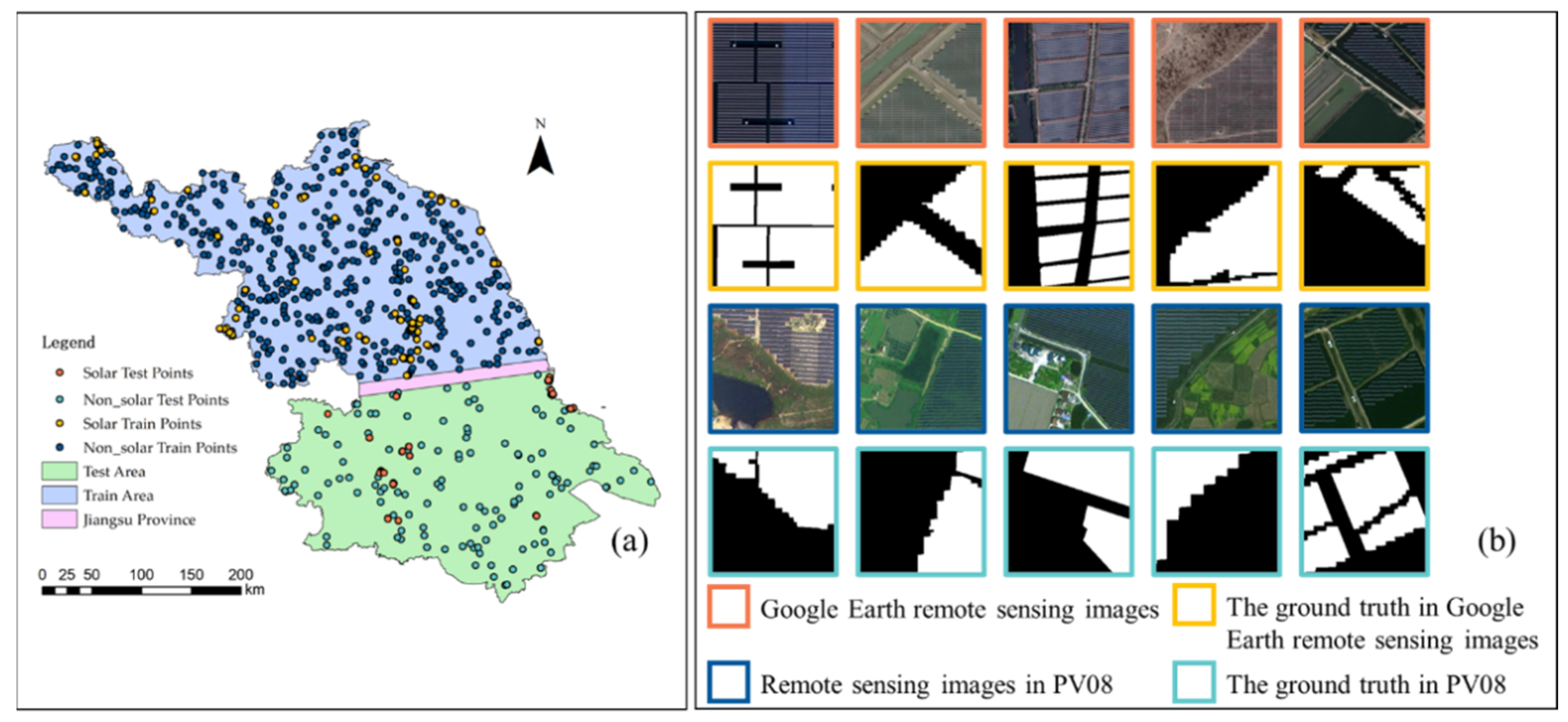
For machine learning, 115 PV observation points from the GPPD [54] database are used to generate buffers using the software ArcMap10.7. Within the 115 buffers, six sample points for each individual buffer are generated randomly. 615/690 (6 × 115) random sample points pass the accuracy check using high-resolution Google Earth imagery and are listed as positive sample points (PV samples). Accordingly, 615 negative samples (non-PV samples) points are randomly selected. Both 615 positive and negative samples are divided into the training set (positive samples: 492, negative samples: 492) and the testing set (positive samples: 123, negative samples: 123); see Figure 5a.
For deep learning, two types of training samples with a pixel size of 256 × 256 are used. Besides 3771 PV samples directly from the PV08 data set [53], 75 PV plant locations are suggested by the GPPD [54] and manually interpreted from high-resolution Google Earth images. 1819 PV plant samples are generated and then rotated by 0°, 90°, 180°, and 270° as training and testing samples in different directions (train: 5604, test: 1672). Together, 9375/11047 (1672/11047) are set as training (testing) samples according to the ratio recommendation of 8:2 [56]., see Figure 5b.

3.2. Machine Learning Broad Spatial Partitioning

Three machine-learning (ML) models, Random Forest (RF), Gradient Boosting Decision Tree (GBDT), and Support Vector Machine (SVM), are compared in PV detection with 394/492 training samples and 98/492 validating samples. Optimized model parameters and feature combinations are calculated (see Section 2.2) and shown in Table 2. The following results are noted:
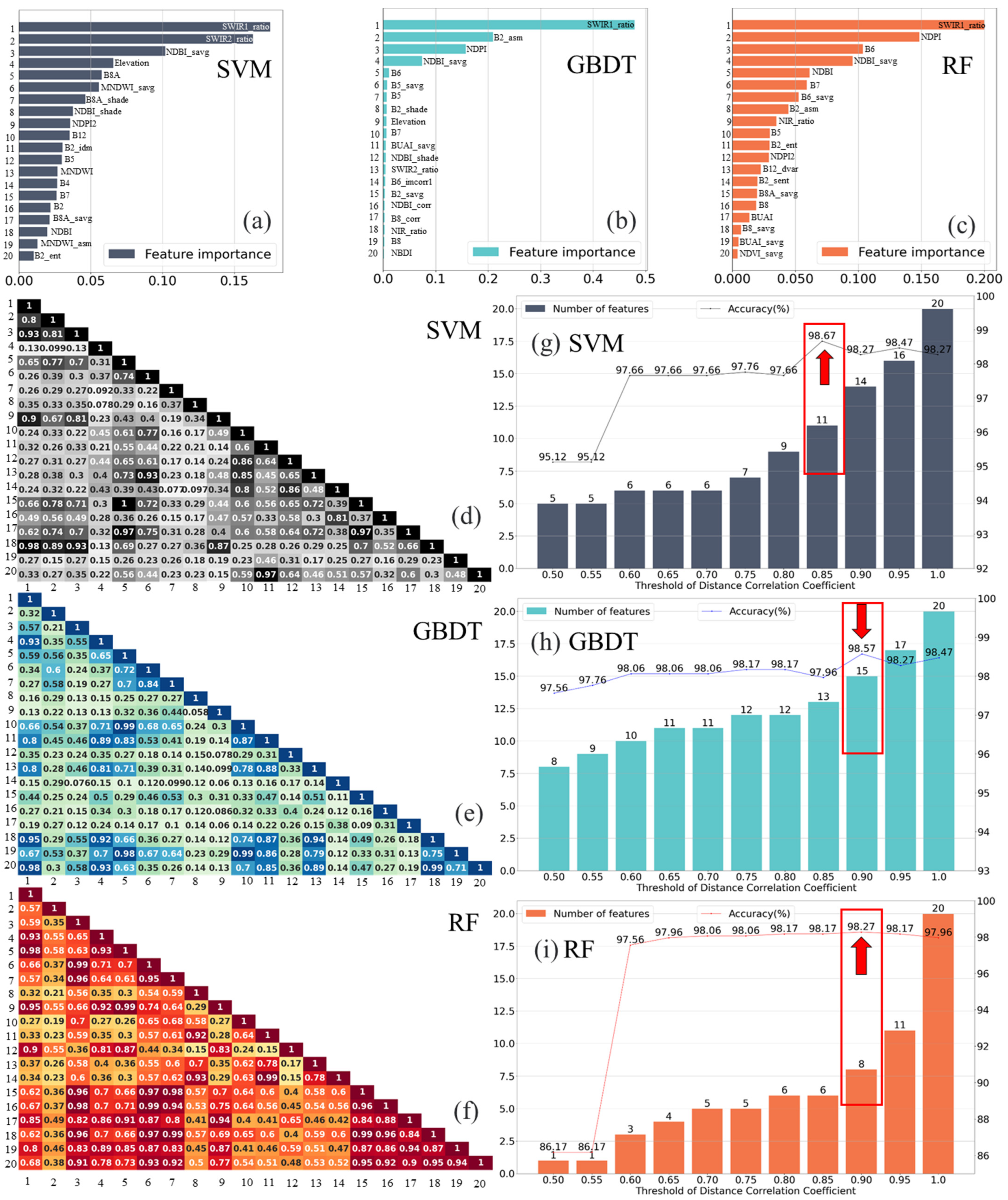
(1) The most important 20 features are selected from 297 candidate features by ML-based Recursive Feature Elimination (RFE, see Section 2.2 and Figure 6a–c). Top four features of GBDT account for PV detection contribution greater than 80%, while feature importance of RF and SVM are more evenly distributed, requiring 9 and 11 features for greater than 80% contribution, respectively.
(2) For all three ML models, the remote sensing index SWIR1_ratrio [40] contributes the most to distinguishing PV plants from the background (RF: ~19.97%, GBDT: ~47.88%, and SVM: ~17.49%). In RF, the contribution of NDPI [39] (~14.84%) is followed by SWIR1_ratio. Spectral features, such as B6 from Sentienl-2, rank on the third importance ~10.36%. Then, Texture characteristic NDBI_savg follows ~9.54%. It is noticeable that the SWIR1_ratio is the ratio of shortwave infrared band 1 to shortwave infrared 1, shortwave infrared 2, and near-infrared bands (see Table 1, 11th row), and the NDBI_savg is the sum average of gray-level co-occurrence matrix (GLCM) for NDBI index (see Table 1, 13th row and Appendix A-Table A2, 6th row). Sentinel-1 has less importance in distinguishing PV plants because none of the features related to Sentinel-1 is in the top 20 list.
(3) The distance correlation coefficients between the selected 20 features represent the similarity or dependency of each two features and range from 0 (light color) to 1 (dark color) in Figure 6d–f. Features selected by RF show significantly higher distance correlation coefficients (see Figure 6f) compared with features selected by GBDT and SVM (see Figure 6d,e). That is, top significance features selected by RF contain a higher redundancy and require further selection.
(4) After iteration validation, accuracy dependencies associated with 11 different feature combinations are shown in Figure 6g–i. The PV detection accuracy increases rapidly at the beginning, then slows down and gradually decreases due to an overfitting phenomenon with the same amount of training data. That is, the models do not necessarily learn more information for distinguishing the PV plants from the background as the number of features increases, but a suitable feature selection is useful for improving the final PV detection accuracy. For SVM, GBDT, and RF, the highest accuracy of 98.67%, 98.57%, and 98.27% occurs with 11, 15, and 8 features, respectively (see Table 2).
Besides accuracy dependencies tested with 98 validation samples, results from three machine learning (ML) models, Random Forest (RF), Gradient Boosting Decision Tree (GBDT), and Support Vector Machine (SVM), are tested with the 123 testing samples. Statistics (see Table 3) and spatial distribution (see Figure 7) indicate the following results:
  • Statistically, results from RF showed the highest overall accuracy (OA) and the highest Kappa value (OA = 95.52%, Kappa = 0.91) compared with results from GBDT (OA = 92.27%, Kappa = 0.84) and SVM (OA = 91.86%, Kappa = 0.83). PV detection results from RF have the highest UApv (95.16%), and background detection results have the highest PAnon-pv (95.12%). That is, RF is a better choice in both PV detection and noise removal. Although GBDT and SVM may extract similar PV plants as RF (PApv and UAnon-pv values ~96%), GBDT and SVM lack the ability to remove noise from the background (see UApv and PAnon-pv less than 90%). Compared with GBDT and SVM, RF uses unbiased estimation for the generalization error and has better generalization. The training data may contain noise, and RF can resist model overfitting, effectively reducing noise interference, so its results are better than GBDT and SVM.
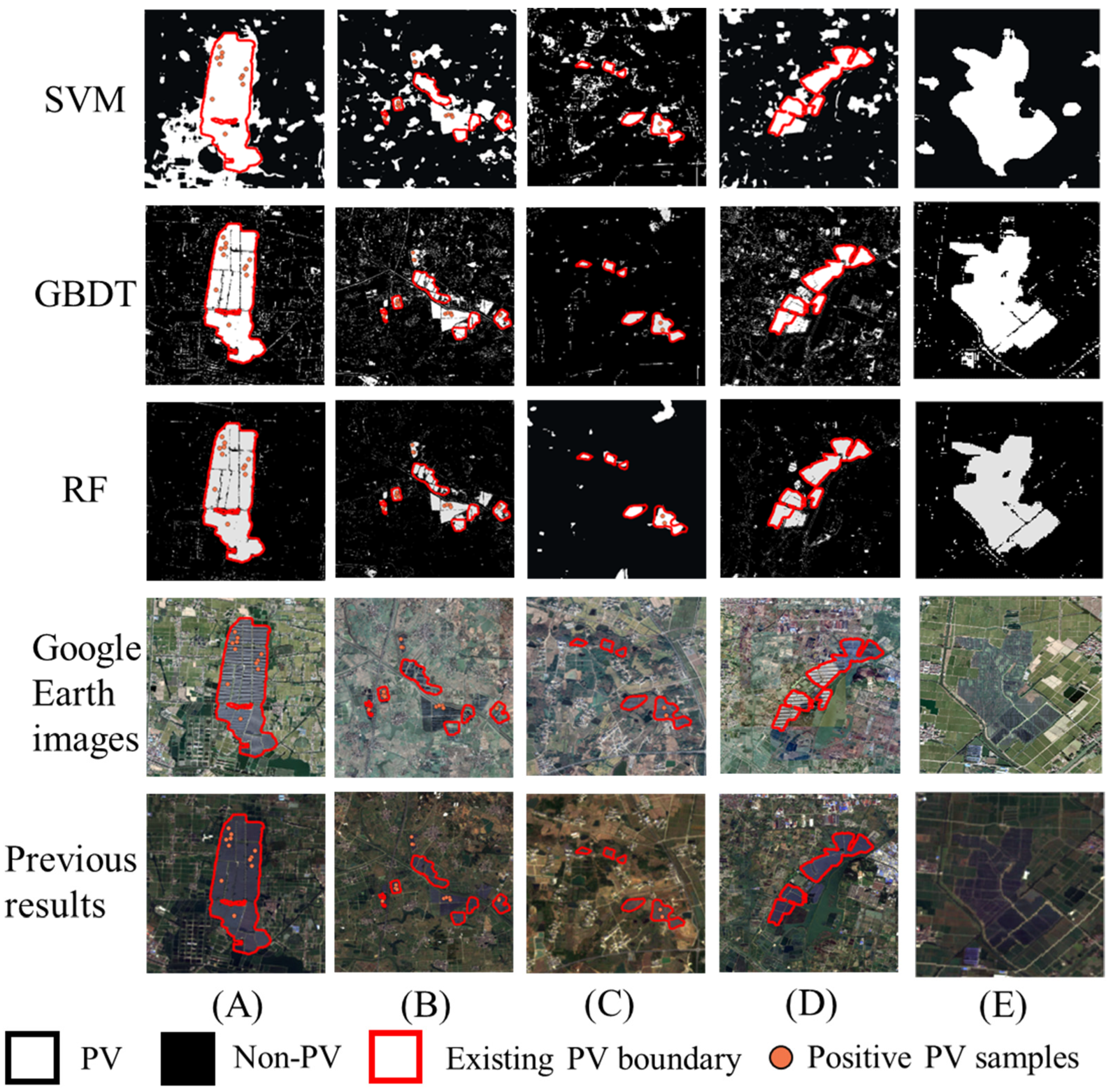
  • Spatially, machine learning broad spatial partitioning from three ML models indicates that missing PV plants in observation data could be diagnosed by those three ML models. However, SVM would be the last choice in PV detection due to the overwhelming noise and unclear detected edges (see 1st row), followed by GBDT with clear boundaries and less noise (see 2nd row), and RF provides even better edges and the best noise suppression (see 3rd row).

3.3. Morphological Processing

RF-based broad spatial partitioning is obtained for subsequent morphological processing for further noise filtering, and the operation kernel of the morphological processing has a radius of 2.5 km. The result shows that more noise could be removed after this opening operation and without PV detection damages (see Figure 8(bA–bC)). Moreover, misclassifications from roads, buildings, and other features as PV plants due to the deficit from the moderate-resolution remote sensing imagery could also be partly eliminated (see Figure 8(bD–bF)). After the morphological opening operation, both the number of pixels (reduced by approximately 2.46 × 10⁷) and vectors (reduced by approximately 1.1 × 10⁵) of PV plants significantly decrease (around 1/3), indicating that this method can effectively reduce a large amount of noise in the extraction results (see Figure 8c).

3.4. Deep Learning Model Comparison

Commonly used deep learning models, such as FCN8S [57], ResUNet34 [58], Deeplabv3+ [59], U2-Net [60], and LANet [61] are used to compare with this improved HRNet methodology (see Section 2.6) using the same sets of training and testing data samples with five times training for each model. Besides, two types of training samples with a pixel size of 256×256 are used: one is from the open access PV samples (PV08 dataset, [53]), and the other is suggested by ground-based PV observations (global power plant database (GPPD), [54]) and manually interpreted from the Google Earth images. The following results are noticed (see Table 4):
  • Selected deep learning models indicate similar evaluation values in terms of Precision and Recall, which means out of all the predicted PV plant pixels, a similar amount (greater than around 95%) are PV plant pixels. Meanwhile, out of all the ground truth PV plants, the models predict a similar amount (greater than 95%) as PV plant pixel, except U2-Net.
  • Selected deep learning models indicate an obvious difference in the evaluation metrics IoU, which measures the overlapped percentage between the predicted results and the ground truth. Compared with commonly used deep learning models, HRNet deep learning diagnostics shows the best performance in terms of evaluation metrics of F1-score (around 96.51%) and IoU (around 93.26%).
  • By integrating sub-pixel convolution, the improved HRNet methodology indicates an improved evaluation value in F1-score (by around 0.23%) and IoU (by around 0.42%). This is because the sub-pixel convolution mitigates the information loss caused by upsampling and thus improves the model performance.
  • Extra PV observations (PV08) are added as training samples applied to the improved HRNet methodology, which helps model performance with the highest evaluation metrics value of F1-score (around 96.95%) and IoU (around 94.08%) and with the highest stability in terms of a low standard deviation (F1-score: 0.03%, IoU: 0.06%).
In general, this improved HRNet has the best performance in PV detection, and the more training samples added, the better the model performance is.

3.5. Detailed Deep Learning Diagnostics

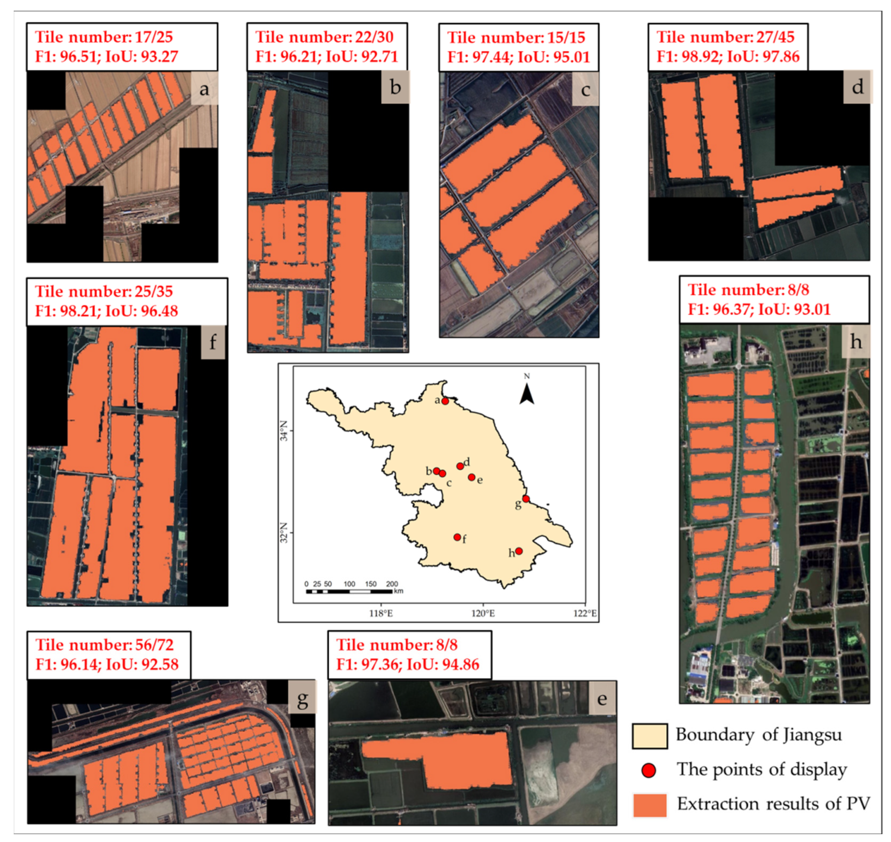
Eight regions with PV plants detected from the improved HRNet are randomly selected and shown in Figure 9. Regional results show evaluation metrics F1-score (IoU) greater than 96% (92%) and almost without noise. This is not only due to the methodology efficiency of the selected deep learning model but also because the tile-selecting step before deep learning reduces the possibility that an application with more tiles may bring more noise. In Figure 9, around 1/3 of the Google Earth tiles without PV plants are eliminated. However, this may bring edge missing issues when some tiles contain little PV edge information (see Figure 9a,d).
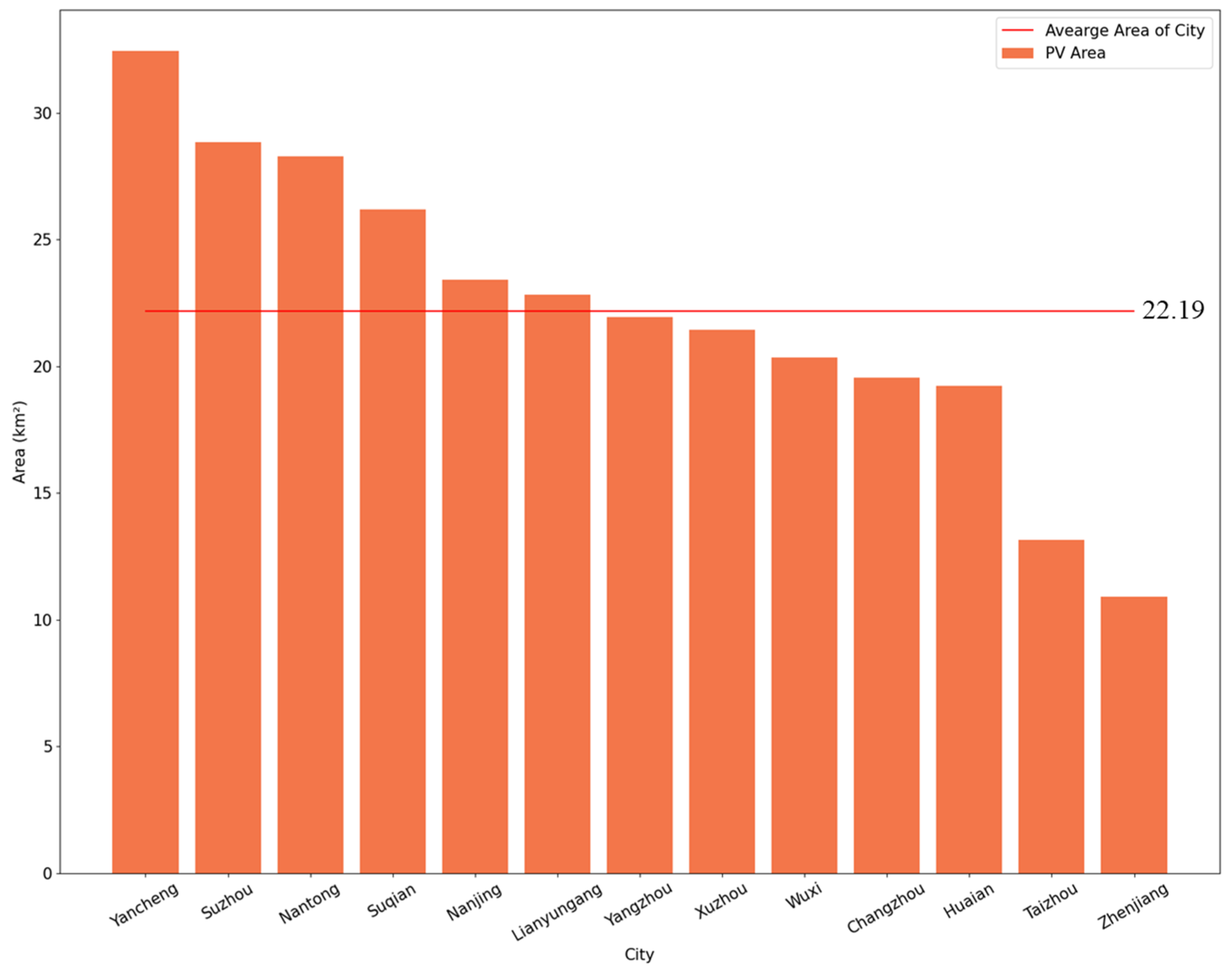
In addition, we conducted a scientific analysis of the PV area in each city of Jiangsu Province in 2022 based on the extraction results of PV plants (see Figure 10). There are thirteen cities in Jiangsu Province. Yancheng City has the largest PV area, approximately 32.44 km2, while Zhenjiang City has the smallest PV area, approximately 10.91 km2. The average PV area across the Jiangsu Province is estimated to be 22.19 km2. The methodology presented in this study has a good reference value in the extraction of PV plants over a large-scale, highly urbanized area.

4. Discussion

Comprising machine learning broad spatial partitioning and detailed deep learning diagnostics, applying suitable feature selection by measuring importance and similarity between candidate features, and removing high-resolution Google Earth tiles without PV plants lead to a novel combinatorial approach to detect PV plants accurately over highly urbanized areas.

4.1. Comparison of Different Feature Selection Methods

Remote sensing observations, spectral indices, texture features, and graphical characteristics are all used as candidate features for supporting separating solar PV plants from the background. However, inputting such a large number of candidate features into the model is time-consuming and may cause recognition performance degradation. The recursive feature elimination with distance correlation coefficient (RFEDCC) used in this study effectively reduces the number of features before the final model training process. Meanwhile, the RFEDCC selects personalized, optimized feature combinations for different models.
To verify the effectiveness of this RFEDCC feature selection method (see Section 2.2), two more feature selection methodologies are compared associated with the Random Forest machine-learning model (RF), including SelectKBest and recursive feature elimination with cross-validation (RFECV) [62]. SelectKBest is a simple method only ranking the feature importance for the RF-based PV detection results. In addition, the key difference between RFECV and RFEDCC is that RFECV (RFEDCC) uses cross-validation (distance correlation coefficient) in (after) the recursive feature elimination process to find the best performance from different feature combinations. Here, to be comparable, the top 8/297 important features are selected for both SelectBest and RFECV, and functions are available in the Python package sklearn (SelectKBest and RFECV).
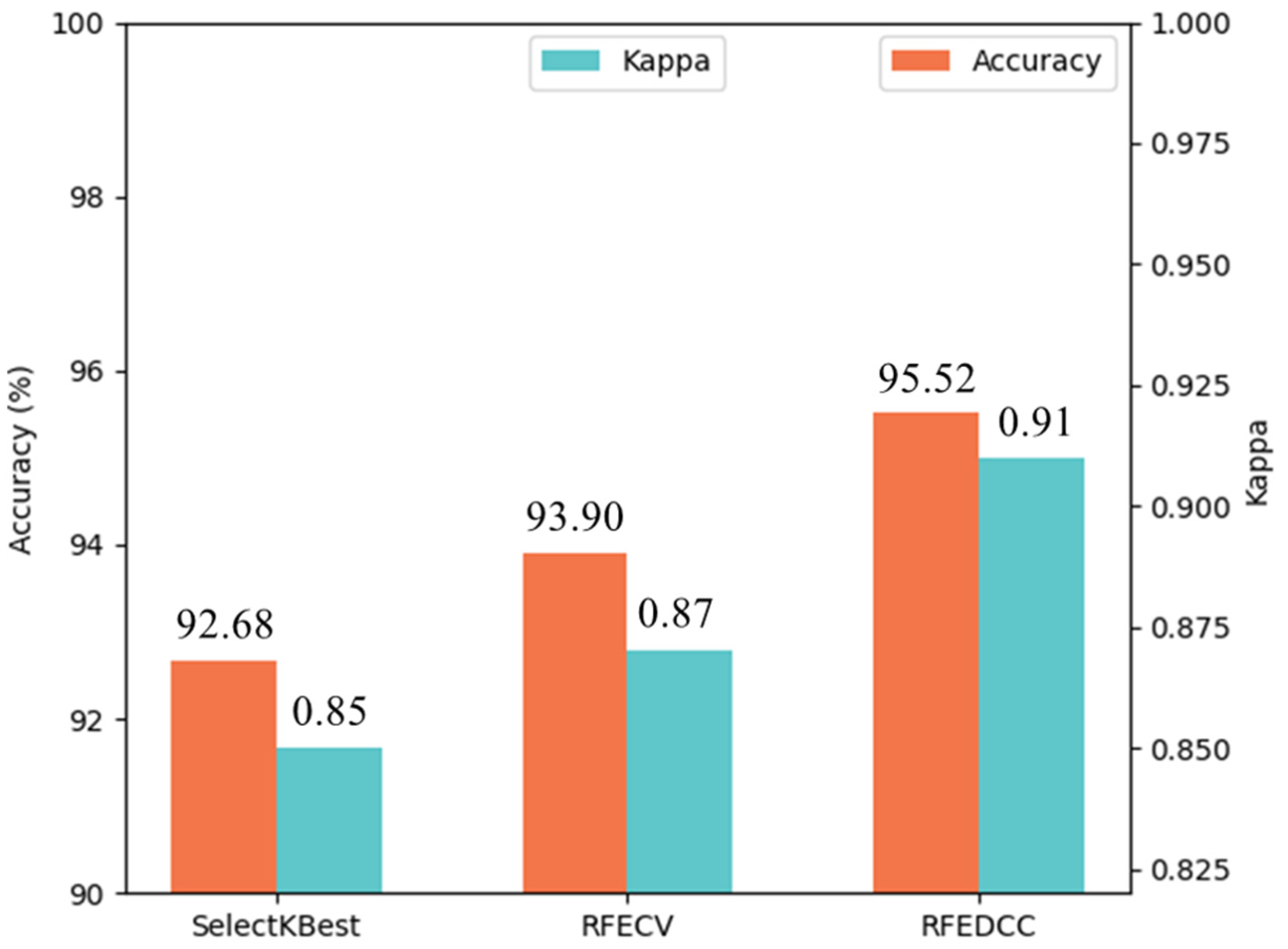
The results (see Figure 11) indicate that features selected by the RFEDCC method achieve a better accuracy (95.52%) and kappa value (0.91) compared with features selected by SelectKBest (Accuracy = 92.68%, Kappa = 0.85) and features selected by RFECV (Accuracy = 93.90%, Kappa = 0.87). This is because the SelectKBest method does not eliminate dependent features but only considers feature importance. In addition, the RFECV method will not be recommended when there is a large number of candidate features because it has to randomly and recursively select and compare all the possible feature combinations. Such a high computational complexity may also cause an overfit result.

4.2. The Effectiveness of Adding Nighttime Light Data

This study focuses on the distribution of PV plants over highly urbanized areas. In reality, PV plants are often built near human residential areas to reduce transmission losses. Thus, previous paper [14] suggests that nighttime light data helps the PV detection in moderate-resolution remote sensing images by detecting PV plants within a predefined urban area (e.g., light intensity greater than 3) with a possible buffer extension (e.g., 15 km radius). In this paper, twelve sets of experiments are designed (the nighttime light intensity threshold = 3, 4, 5, and 6, and the buffer radius = 10 km, 15 km, and 20 km). The result indicates that, unlike the machine learning broad spatial partitioning and a subsequent morphological opening operation, the nighttime light data-based boundary shows limited ability in noising removing, and thus, too many fake possible PV tiles are selected (see Table 5). For example, when the nighttime light intensity threshold is equal to 5, and the buffer is 15 km, only 0.97% of Jiangsu Province could be eliminated. When the nighttime light intensity threshold is greater than 6, some PV plants will be eliminated as well. That is, those fake possible PV tiles decrease the final accuracy for both machine learning broad spatial partitioning and detailed deep learning diagnostics.

4.3. Consistency with Existing PV Database and a Time Consumption Comparison

PV detection results from this two-step downscaling methodology are compared with existing PV distribution from GPPD and from Kruitwagen’s data set [27]. In the original GDDP (Kruitwagen) data, there are 115 (221) PV plant locations (polygons), 112 (204) of which are detected by this two-step downscaling methodology. Thus, the correct detection rate reaches 92.31% and 97.39%, respectively, which is improved compared with a previous study showing the detection rate of GPPD: 86.67% and Kruitwagen: 94.80% for the central and eastern cities in China (see Table 6).
The time consumption of this two-step downscaling methodology compared with a direct improved HRNet deep learning demonstrates that a total of 3,405,795 Google Earth tiles in Jiangsu Province take 309.7 min when applying a direct improved HRNet deep learning, while only 94,020 tiles selected by this two-step downscaling methodology costs 15.2 min in application (see Table 7).
Furthermore, the method proposed by Ge et al., 2022 [31] extracts PV plants in Gansu Province (area: 457,000 km2) in 7.317 h, while our method extracts PV plants in Jiangsu Province (area: 106,000 km2) in 15.2 min. Although Jiangsu Province is approximately 1/5 the area of Gansu Province, our method extracts PV plants only 3/100 of the time reported by Ge et al. [31]. Therefore, our proposed method demonstrates efficiency in terms of time when extracting large-scale PV plants.

5. Conclusions

To complement large-scale PV detection over highly urbanized areas where there are complicated high-density land cover types, a two-step downscaling machine learning broad spatial partitioning and detailed deep learning diagnostics is designed. The following conclusions are noticed:
(1) The RFEDCC is designed for selecting useful features by integrating both feature importance and feature dependence. In the first step, the PV detection results from RF are with an OA (Kappa) of 95.92% (0.91).
(2) Compared with a direct improved HRNet, this two-step methodology reduces around 95% (1–15.2 min/309.7 min) time consumption for extracting Jiangsu Province PV plants.
(3) Nighttime light data used in a similar analysis [14] shows limited ability in abundant tile and noise removal, particularly for highly urbanized areas.
This methodology facilitates large-scale fine PV detection and the continuity of PV condition monitoring. Together with the present PV distribution, the renewable energy generated from PV plants associated with real-time weather conditions will be our phase II study for further contributing to the goal of “Carbon peaking and carbon neutrality”.

Author Contributions

Conceptualization, Y.W. and D.C.; methodology, Y.W. and L.C.; software, Y.W.; validation, Y.W., D.C. and L.C.; formal analysis, Y.W. and X.G.; investigation, Y.W. and X.G.; resources, L.Y.; data curation, Y.W.; writing—original draft preparation, Y.W.; writing—review and editing, D.C.; visualization, Y.W.; supervision, L.P.; project administration, L.Y.; funding acquisition, L.P. All authors have read and agreed to the published version of the manuscript.

Funding

This work was supported by the Energy Foundation, Technology Project: Research on the development potential, influencing factors, and policy recommendations for wind power and distributed photovoltaic new energy in the eastern and central China (G-2305-34616) and the Global Energy Internet Group Co., Ltd., Technology Project: Building Photovoltaic Power Generation Potential Evaluation Method and Empirical Research (SGGEIG00JYJS2100032).

Institutional Review Board Statement

Not applicable.

Informed Consent Statement

Not applicable.

Data Availability Statement

Data and codes used in this study are available from the corresponding author on request.

Acknowledgments

The authors thank the reviewers and editors for their contributions to improving our manuscript.

Conflicts of Interest

The authors declare no conflict of interest.

Appendix A

Table A1. Serial Numbers 1–20 corresponded to the top 20 important features from different machine learning models, including random forest (RF), Gradient Boosting Decision Tree (GBDT), and support vector machine (SVM).
Serial NumberSVMGBDTRF
1SWIR1_ratioSWIR1_ratioSWIR1_ratio
2SWIR2_ratioB2_asmNDPI
3NDBI_savgNDPIB6
4ElevationNDBI_savgNDBI_savg
5B8AB6NDBI
6MNDWI_savgB5_savgB7
7B8A_shadeB5B6_savg
8NDBI_shadeB2_shadeB2_asm
9NDPI2ElevationNIR_ratio
10B12B7B5
11B2_idmBUAI_savgB2_ent
12B5NDBI_shadeNDPI2
13MNDWISWIR2_ratioB12_dvar
14B4B6_imcorr1B2_sent
15B7B2_savgB8A_savg
16B2NDBI_corrB8
17B8A_savgB8_corrBUAI
18NDBINIR_ratioB8_savg
19MNDWI_asmB8BUAI_savg
20B2_entNDBINDVI_savg
Table A2. Detailed name description of Textural Features.
Texture NameFull NameDescription
_asmAngular Second MomentMeasures the number of repeated pairs
_contrastContrastMeasures the local contrast of an image
_corrCorrelationMeasures the correlation between pairs of pixels
_varVarianceMeasures how spread out the distribution of gray levels is
_idmInverse Difference MomentMeasures the homogeneity
_savgSum Average
_svarSum Variance
_sentSum Entropy
_entEntropyMeasures the randomness of a grey-level distribution
_dvarDifference variance
_dentDifference entropy
_imcorr1Information Measure of Corr. 1
_imcorr2Information Measure of Corr. 2
_dissDissimilarity
_inertiaInertia
_shadeCluster Shade
_promCluster prominence

References

  1. The World’s Energy Problem. Available online: https://ourworldindata.org/worlds-energy-problem (accessed on 13 August 2023).
  2. Singh, G.K. Solar power generation by PV (photovoltaic) technology: A review. Energy 2013, 53, 1–13. [Google Scholar]
  3. Timilsina, G.R.; Kurdgelashvili, L.; Narbel, P.A. Solar energy: Markets, economics and policies. Renew. Sustain. Energy Rev. 2012, 16, 449–465. [Google Scholar] [CrossRef]
  4. Abdin, Z.; Alim, M.A.; Saidur, R.; Islam, M.R.; Rashmi, W.; Mekhilef, S.; Wadi, A. Solar energy harvesting with the application of nanotechnology. Renew. Sustain. Energy Rev. 2013, 26, 837–852. [Google Scholar] [CrossRef]
  5. China Energy Portal. Available online: https://chinaenergyportal.org/2021-q2-pv-installations-utility-and-distributed-by-province/ (accessed on 13 August 2023).
  6. Okoye, C.O.; Solyalı, O. Optimal sizing of stand-alone photovoltaic systems in residential buildings. Energy 2017, 126, 573–584. [Google Scholar] [CrossRef]
  7. Chen, Y.; Lin, Z.; Zhao, X.; Wang, G.; Gu, Y. Deep learning-based classification of hyperspectral data. IEEE J. Sel. Top. Appl. Earth Obs. Remote Sens. 2014, 7, 2094–2107. [Google Scholar] [CrossRef]
  8. Thoreau, R.; Achard, V.; Risser, L.; Berthelot, B.; Briottet, X. Active learning for hyperspectral image classification: A comparative review. IEEE Geosci. Remote Sens. Mag. 2022, 10, 256–278. [Google Scholar] [CrossRef]
  9. Rangarajan, A.K.; Whetton, R.L.; Mouazen, A.M. Detection of fusarium head blight in wheat using hyperspectral data and deep learning. Expert Syst. Appl. 2022, 208, 118240. [Google Scholar] [CrossRef]
  10. Chen, Z.; Kang, Y.; Sun, Z.; Wu, F.; Zhang, Q. Extraction of Photovoltaic Plants Using Machine Learning Methods: A Case Study of the Pilot Energy City of Golmud, China. Remote Sens. 2022, 14, 2697. [Google Scholar] [CrossRef]
  11. Zhang, H.; Tian, P.; Zhong, J.; Liu, Y.; Li, J. Mapping Photovoltaic Panels in Coastal China Using Sentinel-1 and Sentinel-2 Images and Google Earth Engine. Remote Sens. 2023, 15, 3712. [Google Scholar] [CrossRef]
  12. Xia, Z.; Li, Y.; Chen, R.; Sengupta, D.; Guo, X.; Xiong, B.; Niu, Y. Mapping the rapid development of photovoltaic power stations in northwestern China using remote sensing. Energy Rep. 2022, 8, 4117–4127. [Google Scholar] [CrossRef]
  13. Belgiu, M.; Drăguţ, L. Random forest in remote sensing: A review of applications and future directions. ISPRS J. Photogramm. Remote Sens. 2016, 114, 24–31. [Google Scholar] [CrossRef]
  14. Wang, J.; Liu, J.; Li, L. Detecting Photovoltaic Installations in Diverse Landscapes Using Open Multi-Source Remote Sensing Data. Remote Sens. 2022, 14, 6296. [Google Scholar] [CrossRef]
  15. Zhao, H.; Yin, Z. Remote Sensing Extraction of Photovoltaic Panels in Desert Areas Based on Feature Optimization. In Proceedings of the 2022 15th International Congress on Image and Signal Processing, BioMedical Engineering and Informatics (CISP-BMEI), Beijing, China, 5–7 November 2022; pp. 1–6. [Google Scholar]
  16. Plakman, V.; Rosier, J.; van Vliet, J. Solar park detection from publicly available satellite imagery. GISci. Remote Sens. 2022, 59, 462–481. [Google Scholar] [CrossRef]
  17. Cui, W.; Wang, F.; He, X.; Zhang, D.; Xu, X.; Yao, M.; Wang, Z.; Huang, J. Multi-scale semantic segmentation and spatial relationship recognition of remote sensing images based on an attention model. Remote Sens. 2019, 11, 1044. [Google Scholar] [CrossRef]
  18. Venkatesh, B.; Anuradha, J. A review of feature selection and its methods. Cybern. Inf. Technol. 2019, 19, 3–26. [Google Scholar] [CrossRef]
  19. Jianxun, W.; Xin, C.; Weicheng, J.; Li, H.; Junyi, L.; Haigang, S. PVNet: A novel semantic segmentation model for extracting high-quality photovoltaic panels in large-scale systems from high-resolution remote sensing imagery. Int. J. Appl. Earth Obs. Geoinf. 2023, 119, 103309. [Google Scholar]
  20. Jie, Y.; Yue, A.; Liu, S.; Huang, Q.; Chen, J.; Meng, Y.; Deng, Y.; Yu, Z. Photovoltaic power station identification using refined encoder–decoder network with channel attention and chained residual dilated convolutions. J. Appl. Remote Sens. 2020, 14, 016506. [Google Scholar] [CrossRef]
  21. Pérez-González, A.; Jaramillo-Duque, Á.; Cano-Quintero, J.B. Automatic boundary extraction for photovoltaic plants using the deep learning U-net model. Appl. Sci. 2021, 11, 6524. [Google Scholar] [CrossRef]
  22. Jie, Y.; Ji, X.; Yue, A.; Chen, J.; Deng, Y.; Chen, J.; Zhang, Y. Combined multi-layer feature fusion and edge detection method for distributed photovoltaic power station identification. Energies 2020, 13, 6742. [Google Scholar] [CrossRef]
  23. Su, B.; Du, X.; Mu, H.; Xu, C.; Li, X.; Chen, F.; Luo, X. FEPVNet: A Network with Adaptive Strategies for Cross-Scale Mapping of Photovoltaic Panels from Multi-Source Images. Remote Sens. 2023, 15, 2469. [Google Scholar] [CrossRef]
  24. Zhu, R.; Guo, D.; Wong, M.S.; Qian, Z.; Chen, M.; Yang, B.; Chen, B.; Zhang, H.; You, L.; Heo, J. Deep solar PV refiner: A detail-oriented deep learning network for refined segmentation of photovoltaic areas from satellite imagery. Int. J. Appl. Earth Obs. Geoinf. 2023, 116, 103134. [Google Scholar] [CrossRef]
  25. Chen, Q.; Li, X.; Zhang, Z.; Zhou, C.; Guo, Z.; Liu, Z.; Zhang, H. Remote sensing of photovoltaic scenarios: Techniques, applications and future directions. Appl. Energy 2023, 333, 120579. [Google Scholar] [CrossRef]
  26. Malof, J.M.; Collins, L.M.; Bradbury, K.; Newell, R.G. A deep convolutional neural network and a random forest classifier for solar photovoltaic array detection in aerial imagery. In Proceedings of the 2016 IEEE International Conference on Renewable Energy Research and Applications (ICRERA), Birmingham, UK, 20–23 November 2016; pp. 650–654. [Google Scholar]
  27. Kruitwagen, L.; Story, K.; Friedrich, J.; Byers, L.; Skillman, S.; Hepburn, C. A global inventory of photovoltaic solar energy generating units. Nature 2021, 598, 604–610. [Google Scholar] [CrossRef] [PubMed]
  28. Ronneberger, O.; Fischer, P.; Brox, T. U-net: Convolutional networks for biomedical image segmentation. In Medical Image Computing and Computer-Assisted Intervention–MICCAI 2015: 18th International Conference, Munich, Germany, October 5–9, 2015, Proceedings, Part III 18; Springer: Cham, Switzerland, 2015; pp. 234–241. [Google Scholar]
  29. Yu, J.; Wang, Z.; Majumdar, A.; Rajagopal, R. DeepSolar: A machine learning framework to efficiently construct a solar deployment database in the United States. Joule 2018, 2, 2605–2617. [Google Scholar] [CrossRef]
  30. Szegedy, C.; Vanhoucke, V.; Ioffe, S.; Shlens, J.; Wojna, Z. Rethinking the inception architecture for computer vision. In Proceedings of the IEEE Conference on Computer Vision and Pattern Recognition, Las Vegas, NV, USA, 27–30 June 2016; pp. 2818–2826. [Google Scholar]
  31. Ge, F.; Wang, G.; He, G.; Zhou, D.; Yin, R.; Tong, L. A Hierarchical Information Extraction Method for Large-Scale Centralized Photovoltaic Power Plants Based on Multi-Source Remote Sensing Images. Remote Sens. 2022, 14, 4211. [Google Scholar] [CrossRef]
  32. Fan, L.; Chen, D.; Fu, C.; Yan, Z. Statistical downscaling of summer temperature extremes in northern China. Adv. Atmos. Sci. 2013, 30, 1085–1095. [Google Scholar] [CrossRef]
  33. Wilby, R.L.; Wigley, T.; Conway, D.; Jones, P.; Hewitson, B.; Main, J.; Wilks, D. Statistical downscaling of general circulation model output: A comparison of methods. Water Resour. Res. 1998, 34, 2995–3008. [Google Scholar] [CrossRef]
  34. Xu, Z.; Han, Y.; Tam, C.-Y.; Yang, Z.-L.; Fu, C. Bias-corrected CMIP6 global dataset for dynamical downscaling of the historical and future climate (1979–2100). Sci. Data 2021, 8, 293. [Google Scholar] [CrossRef] [PubMed]
  35. Zha, Y.; Gao, J.; Ni, S. Use of normalized difference built-up index in automatically mapping urban areas from TM imagery. Int. J. Remote Sens. 2003, 24, 583–594. [Google Scholar] [CrossRef]
  36. Tucker, C.J. Red and photographic infrared linear combinations for monitoring vegetation. Remote Sens. Environ. 1979, 8, 127–150. [Google Scholar] [CrossRef]
  37. Xu, H. Modification of normalised difference water index (NDWI) to enhance open water features in remotely sensed imagery. Int. J. Remote Sens. 2006, 27, 3025–3033. [Google Scholar] [CrossRef]
  38. Li, W. Study on Extraction Methods of Impervious Surface Information Extraction from Urban Area Using Remote Sensing. Master’s Thesis, North University of China, Taiyuan, China, 2013. [Google Scholar]
  39. Wang, S. Application of Machine Learning Method in Remote Sensing Extraction of Photovoltaic Power Plants. Master’s Thesis, Jiangsu Normal University, Xuzhou, China, 2018. [Google Scholar]
  40. Wang, S.; Zhang, L.; Zhu, S.; Ji, L.; Chai, Q.; Shen, Y.; Zhang, R. Multi-invariant Feature Combined Photovoltaic Power Plants Extraction Using Multi-temporal Landsat 8 OLI Imagery. Bull. Surv. Mapp. 2018, 11, 46–52. [Google Scholar] [CrossRef]
  41. Haralick, R.M.; Shanmugam, K.; Dinstein, I.H. Textural features for image classification. IEEE Trans. Syst. Man Cybern. 1973, 6, 610–621. [Google Scholar] [CrossRef]
  42. Ji, C.; Bachmann, M.; Esch, T.; Feilhauer, H.; Heiden, U.; Heldens, W.; Hueni, A.; Lakes, T.; Metz-Marconcini, A.; Schroedter-Homscheidt, M. Solar photovoltaic module detection using laboratory and airborne imaging spectroscopy data. Remote Sens. Environ. 2021, 266, 112692. [Google Scholar] [CrossRef]
  43. Zhang, M.; Du, J.; Luo, J.; Nie, B.; Xiong, W.; Liu, M.; Zhao, S. Research on Feature Selection of Multi-Objective Optimization. Comput. Eng. Appl. 2023, 59, 23–32. [Google Scholar] [CrossRef]
  44. Breiman, L. Random forests. Mach. Learn. 2001, 45, 5–32. [Google Scholar] [CrossRef]
  45. Friedman, J.H. Greedy function approximation: A gradient boosting machine. Ann. Stat. 2001, 29, 1189–1232. [Google Scholar] [CrossRef]
  46. Cortes, C.; Vapnik, V. Support-vector networks. Mach. Learn. 1995, 20, 273–297. [Google Scholar] [CrossRef]
  47. Van Horebeek, J.; Tapia-Rodriguez, E. The approximation of a morphological opening and closing in the presence of noise. Signal Process. 2001, 81, 1991–1995. [Google Scholar] [CrossRef]
  48. Tile Map Service Specification. Available online: https://wiki.osgeo.org/wiki/Tile_Map_Service_Specification (accessed on 5 June 2023).
  49. Sun, K.; Zhao, Y.; Jiang, B.; Cheng, T.; Xiao, B.; Liu, D.; Mu, Y.; Wang, X.; Liu, W.; Wang, J. High-resolution representations for labeling pixels and regions. arXiv 2019, arXiv:1904.04514. [Google Scholar]
  50. Lin, T.-Y.; Dollár, P.; Girshick, R.; He, K.; Hariharan, B.; Belongie, S. Feature pyramid networks for object detection. In Proceedings of the IEEE Conference on Computer Vision and Pattern Recognition, Honolulu, HI, USA, 21–26 July 2017; pp. 2117–2125. [Google Scholar]
  51. Shamshiri, R.; Eide, E.; Høyland, K.V. Spatio-temporal distribution of sea-ice thickness using a machine learning approach with Google Earth Engine and Sentinel-1 GRD data. Remote Sens. Environ. 2022, 270, 112851. [Google Scholar] [CrossRef]
  52. Electricity Consumption of the Whole Society in Jiangsu Province by Region in 2021. Available online: http://stats.jiangsu.gov.cn/2022/nj09/nj0910.htm (accessed on 5 August 2023).
  53. Jiang, H.; Yao, L.; Lu, N.; Qin, J.; Liu, T.; Liu, Y.; Zhou, C. Multi-resolution dataset for photovoltaic panel segmentation from satellite and aerial imagery. Earth Syst. Sci. Data 2021, 13, 5389–5401. [Google Scholar] [CrossRef]
  54. Global Power Plant Database. Available online: https://datasets.wri.org/dataset/globalpowerplantdatabase (accessed on 20 June 2023).
  55. Farr, T.G.; Rosen, P.A.; Caro, E.; Crippen, R.; Duren, R.; Hensley, S.; Kobrick, M.; Paller, M.; Rodriguez, E.; Roth, L. The shuttle radar topography mission. Rev. Geophys. 2007, 45, RG2004. [Google Scholar] [CrossRef]
  56. Zhang, X.; Cheng, B.; Chen, J.; Liang, C. High-resolution boundary refined convolutional neural network for automatic agricultural greenhouses extraction from gaofen-2 satellite imageries. Remote Sens. 2021, 13, 4237. [Google Scholar] [CrossRef]
  57. Long, J.; Shelhamer, E.; Darrell, T. Fully convolutional networks for semantic segmentation. In Proceedings of the IEEE Conference on Computer Vision and Pattern Recognition, Boston, MA, USA, 7–12 June 2015; pp. 3431–3440. [Google Scholar]
  58. Zhang, Z.; Liu, Q.; Wang, Y. Road extraction by deep residual u-net. IEEE Geosci. Remote Sens. Lett. 2018, 15, 749–753. [Google Scholar] [CrossRef]
  59. Chen, L.-C.; Zhu, Y.; Papandreou, G.; Schroff, F.; Adam, H. Encoder-decoder with atrous separable convolution for semantic image segmentation. In Proceedings of the European Conference on Computer Vision (ECCV), Munich, Germany, 8–14 September 2018; pp. 801–818. [Google Scholar]
  60. Qin, X.; Zhang, Z.; Huang, C.; Dehghan, M.; Zaiane, O.R.; Jagersand, M. U2-Net: Going deeper with nested U-structure for salient object detection. Pattern Recognit. 2020, 106, 107404. [Google Scholar] [CrossRef]
  61. Ding, L.; Tang, H.; Bruzzone, L. LANet: Local attention embedding to improve the semantic segmentation of remote sensing images. IEEE Trans. Geosci. Remote Sens. 2020, 59, 426–435. [Google Scholar] [CrossRef]
  62. Wu, J.; Zheng, D.; Wu, Z.; Song, H.; Zhang, X. Prediction of Buckwheat Maturity in UAV-RGB Images Based on Recursive Feature Elimination Cross-Validation: A Case Study in Jinzhong, Northern China. Plants 2022, 11, 3257. [Google Scholar] [CrossRef]
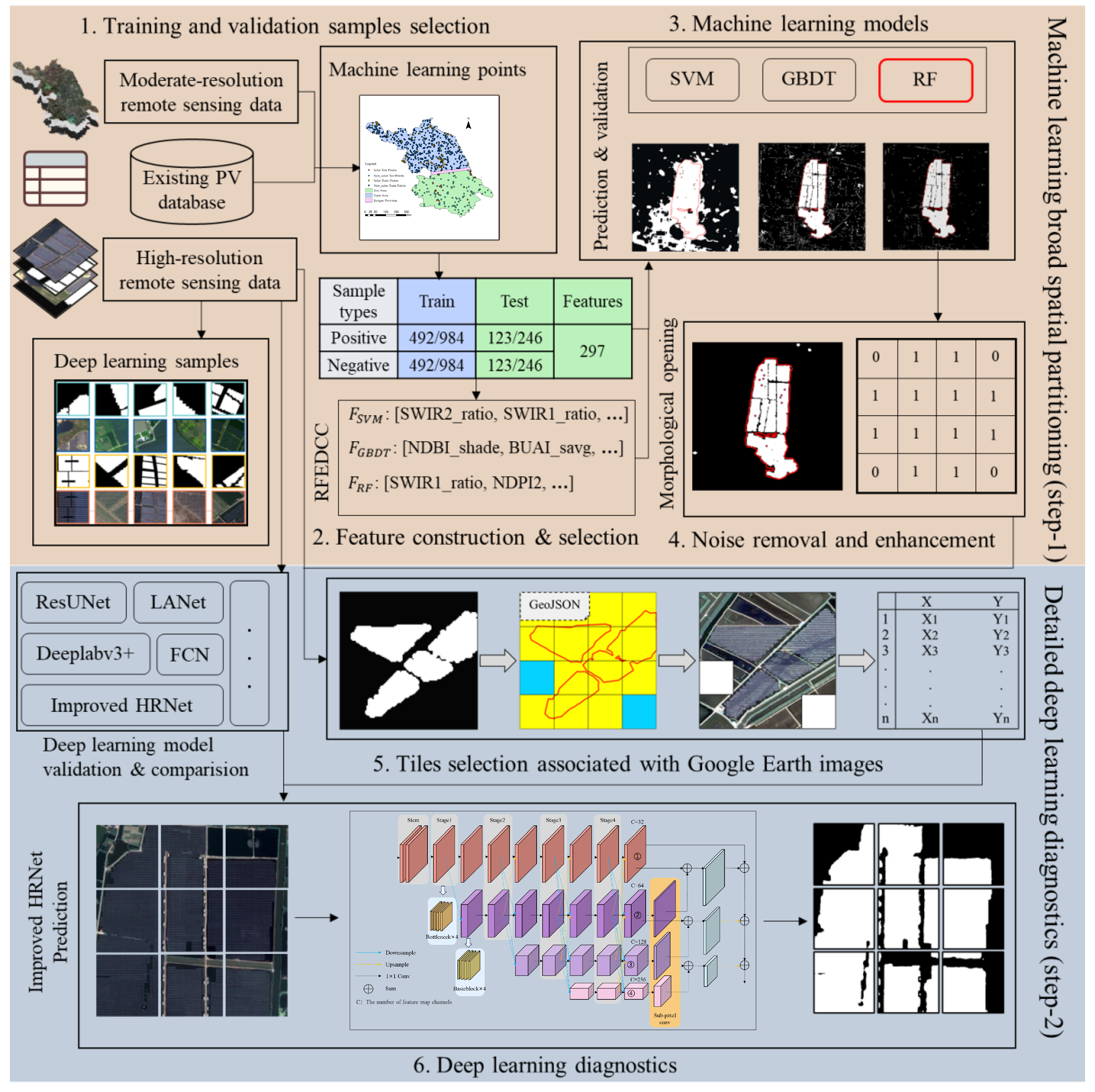
Figure 1. A flowchart illustrating six stages of photovoltaic plant (PV) detection in this study.
Remotesensing 15 04931 g001
Figure 2. The selection process for Google Earth tiles.
Remotesensing 15 04931 g002
Figure 3. Illustrating the architecture of (a) improved HRNet and the details of (b) sub-pixel convolution. The rectangular blocks represent the feature maps, and ‘→’ represents the sub-pixel convolution operation.
Remotesensing 15 04931 g003
Figure 4. Study area overview: The Sentinel-2 satellite true color composite image of (b) Jiangsu Province in (a) China. The 2021 (c) electricity consumption of the whole society, and (d) the potential of photovoltaic power generation in Jiangsu Province.
Remotesensing 15 04931 g004
Figure 5. The (a) machine-learning sample points in Jiangsu Province and part of the (b) semantic segmentation data set display.
Remotesensing 15 04931 g005
Figure 6. Illustration of the feature selection from machine learning-based feature importance ranking (top 20, ac) to distance correlation coefficients calculation (df) and to the iteration validation (gi, see also Section 2.2). Related results are listed as SVM (a,d,g), GBDT (b,e,h), and RF (c,f,i). Note that the highest accuracy is highlighted with red arrows, and the legend of 1~20 is explained in Appendix A, Table A2.
Remotesensing 15 04931 g006
Figure 7. Photovoltaic (PV) prediction results from a comparison of three machine learning models with a spatial resolution of 10 m: support vector machine (SVM, 1st row), gradient boosting decision tree (GBDT 2nd row), and random forest (RF, 3rd row). Meanwhile, the above-mentioned prediction results are compared with Google Earth images with a spatial resolution of 0.54 m (4th row) and with the previous PV database (red boundary in 5th row, see Kruitwagen et al. [27]). Note that the test samples are also highlighted with yellow points, and the five displayed locations are: (A) 119.51°E, 31.84°N; (B) 119.39°E, 31.95°N; (C) 118.91°E, 32.47°N; (D) 119.65°E, 31.51°N; (E) 119.51°E, 31.91°N.
Remotesensing 15 04931 g007
Figure 8. The results of RF photovoltaic (PV) plant extraction in Jiangsu Province as a (a) whole and (b) locally processed after morphological opening operation and the comparison (c) of the number of pixels and shapefile before and after morphological operation.
Remotesensing 15 04931 g008
Figure 9. Eight regions with PV plants detected from the improved HRNet with the legend of evaluation metrics F1-score and IoU. Black means the tile is without possible PV plants (see Section 2.5 Filtering associated with Google Earth Images).
Remotesensing 15 04931 g009
Figure 10. Photovoltaic area of each city in Jiangsu Province.
Remotesensing 15 04931 g010
Figure 11. Comparison of RFECV (recursive feature elimination with cross-validation), SelectKBest, and RFEDCC (recursive feature elimination with distance correlation coefficient) feature selection method.
Remotesensing 15 04931 g011
Table 1. The downscaling methodology inputs for identifying solar PV power systems include remote sensing observations and retrieves (spectral indices, texture features, and geographical characteristics).
TypesAttributesDetailsMethod
Remote Sensing
Observations
Reflectance
Polarization
DEM
Remote Sensing
Retrieves
Remote Sensing
Index
NDBI [35] ( S W I R 1 N I R ) / ( S W I R 1 + N I R )
NDVI [36] ( N I R R e d ) / ( N I R + R e d )
MNDWI [37] ( G r e e n S W I R 1 ) / ( G r e e n + S W I R 1 )
BUAI [38] N D B I N D V I
NDPI [39] ( S W I R 1 N I R ) / ( N I R S W I R 2 )
NDPI2 [39] ( S W I R 1 N I R ) / R e d
NIR_ratio [40] N I R / ( N I R + S W I R 1 + S W I R 2 )
SWIR1_ratio [40] S W I R 1 / ( N I R + S W I R 1 + S W I R 2 )
SWIR2_ratio [40] S W I R 2 / ( N I R + S W I R 1 + S W I R 2 )
Texture [41]glcmTexture() function in GEE (kernel size = 8)
Geographical
Characteristics
Slope, Aspect,
Hillshade.
ee.Terrain.slope(), ee.Terrain.aspect(), and ee.Terrain.hillshade() function in GEE
Table 2. Feature selection results for support vector machine (SVM), gradient boosting decision tree (GBDT), and random forest (RF) by RFEDCC (recursive feature elimination with distance correlation coefficient). The features are ranked in descending order of feature importance.
ModelParameter SettingNumber of
Selected Features
Detailed Features
SVMdecisionProcedure = ’Voting’,
svmType = ’C_SVC’,
KernelType = ’LINEAR’, const = 1.
11SWIR1_ratio, SWIR2_ratio, Elevation, B8A,
MNDWI_savg, B8A_shade, NDBI_shade,
B12, B2_idm, B2, MNDWI_asm.
GBDTnumberOfTrees = 127,
shrinkage = 0.005, seed = 42, loss = ’LeastAbsoluteDeviation’.
15SWIR1_ratio, B2_asm, NDPI, B6, B5_savg, B5,
B2_shade, Elevation, BUAI_savg, NDBI_shade,
SWIR2_ratio, B6_imcorr1, B2_savg, NDBI_corr,
B8_corr.
RFnumberOfTrees = 71,
critertion = ‘gini’, seed = 42.
8SWIR1_ratio, NDPI, B6, B2_asm, B5, NDPI2,
B12_dvar, BUAI_savg.
Table 3. Results of support vector machine (SVM), gradient boosting decision tree (GBDT), and random forest (RF) on test sets after training with features selected by recursive feature elimination with distance correlation coefficient (RFEDCC).
ModelOA (%)KappaUAnon-pv (%)PAnon-pv (%)UApv (%)PApv (%)
SVM91.860.8396.3986.9988.1496.74
GBDT92.270.8495.6188.6189.3995.93
RF95.520.9195.9195.1295.1695.93
Note: The best performances are marked as bold.
Table 4. Comparison of the deep learning models (mean ± standard deviation).
ModelAccuracy (%)Precision (%)Recall (%)F1-Score (%)IoU (%)
FCN8S [57]95.98 ± 0.1894.92 ± 0.2195.34 ± 0.5795.13 ± 0.2390.17 ± 0.42
ResUNet34 [58]96.88 ± 0.1296.85 ± 0.5795.53 ± 0.4796.18 ± 0.1492.65 ± 0.25
Deeplabv3+ [59]96.73 ± 0.1695.39 ± 0.3496.73 ± 0.5196.05 ± 0.2192.41 ± 0.36
U2-Net [60]93.01 ± 1.5695.65 ± 0.3486.97 ± 3.8891.07 ± 2.1883.65 ± 3.64
LANet [61]96.22 ± 0.1395.41 ± 0.4895.42 ± 0.3195.41 ± 0.1591.22 ± 0.28
HRNet [49]97.12 ± 0.1696.32 ± 0.1596.71 ± 0.3196.51 ± 0.2193.26 ± 0.37
Ours97.31 ± 0.0996.33 ± 0.2197.14 ± 0.3296.74 ± 0.1193.68 ± 0.21
Ours+97.47 ± 0.0396.45 ± 0.0697.45 ± 0.0496.95 ± 0.0394.08 ± 0.06
Note: The best performance is marked as bold. +: Extra PV observations (PV08) are added as training data.
Table 5. Experimental results with different nighttime light intensity thresholds and buffer radius. Numbers within the table are area-eliminated percentages for a further step of deep learning (%). Marks show whether PV plants are mistakenly eliminated by the threshold setting (√: only background eliminated, ×: PV plants mistakenly eliminated)).
Radius (km)Intensity Threshold (nanoWatts/sr/cm2)
3 (%)4 (%)5 (%)6 (%)
101.30/√2.51/×4.05/×6.98/×
150.31/√0.49/√0.97/√1.82/×
200.05/√0.06/√0.12/√0.45/×
Table 6. Consistency of our detection with existing PV database.
Reference DatabaseNumber of PVDetectionDetection Rate (%)
GPPD11511292.31
Kruitwagen et al., 2021 [27]22120497.39
Table 7. Time spent for PV plant extraction in Jiangsu Province by deep learning (DL) and our method.
MethodNumber of Tiles (all)Number of Tiles (selected)Time Consumption
DL 3,405,795309.7 min
Ours Method3,405,79594,02015.2 min
Disclaimer/Publisher’s Note: The statements, opinions and data contained in all publications are solely those of the individual author(s) and contributor(s) and not of MDPI and/or the editor(s). MDPI and/or the editor(s) disclaim responsibility for any injury to people or property resulting from any ideas, methods, instructions or products referred to in the content.