Comparison of Deep Neural Networks in the Classification of Bark Beetle-Induced Spruce Damage Using UAS Images ^†

Abstract

The widespread tree mortality caused by the European spruce bark beetle (Ips typographus L.) is a significant concern for Norway spruce-dominated (Picea abies H. Karst) forests in Europe and there is evidence of increases in the affected areas due to climate warming. Effective forest monitoring methods are urgently needed for providing timely data on tree health status for conducting forest management operations that aim to prepare and mitigate the damage caused by the beetle. Unoccupied aircraft systems (UASs) in combination with machine learning image analysis have emerged as a powerful tool for the fast-response monitoring of forest health. This research aims to assess the effectiveness of deep neural networks (DNNs) in identifying bark beetle infestations at the individual tree level from UAS images. The study compares the efficacy of RGB, multispectral (MS), and hyperspectral (HS) imaging, and evaluates various neural network structures for each image type. The findings reveal that MS and HS images perform better than RGB images. A 2D-3D-CNN model trained on HS images proves to be the best for detecting infested trees, with an F1-score of 0.759, while for dead and healthy trees, the F1-scores are 0.880 and 0.928, respectively. The study also demonstrates that the tested classifier networks outperform the state-of-the-art You Only Look Once (YOLO) classifier module, and that an effective analyzer can be implemented by integrating YOLO and the DNN classifier model. The current research provides a foundation for the further exploration of MS and HS imaging in detecting bark beetle disturbances in time, which can play a crucial role in forest management efforts to combat large-scale outbreaks. The study highlights the potential of remote sensing and machine learning in monitoring forest health and mitigating the impacts of biotic stresses. It also offers valuable insights into the effectiveness of DNNs in detecting bark beetle infestations using UAS-based remote sensing technology.

1. Introduction

The changing climate has resulted in an increase in forest damage globally, with extreme weather events, wildfires, and insect disturbances being the main contributing factors [1,2,3]. One of the most destructive forest pests is the European spruce bark beetle (Ips typographus L.), which has benefitted from the warming climate as it provides opportunities for the development of additional generations during a single growing season due to the temperature dependence of bark beetle development [4,5]. This bark beetle has already caused vast tree mortality in central Europe, southern Sweden, and Russia, and large-scale tree mortality events are witnessed increasingly at higher latitudes [3]. Extensive tree mortality causes great economical, ecological, and social losses [6] that can be mitigated by means of forest management and the monitoring of forest health [7].

To effectively monitor and manage forest pests, the accurate and timely detection of damaged trees is essential. Traditional methods of detecting bark beetle damage have involved in situ visual inspections, which are time consuming, inefficient, and challenging for large forest areas [8,9]. Remote sensing technologies have emerged as a promising alternative, offering the potential for the timely and accurate identification of affected trees over large areas. Unoccupied aircraft systems (UASs) can promptly acquire the high-resolution imagery data of forests, making them an attractive tool for monitoring and estimating forest health [10,11].

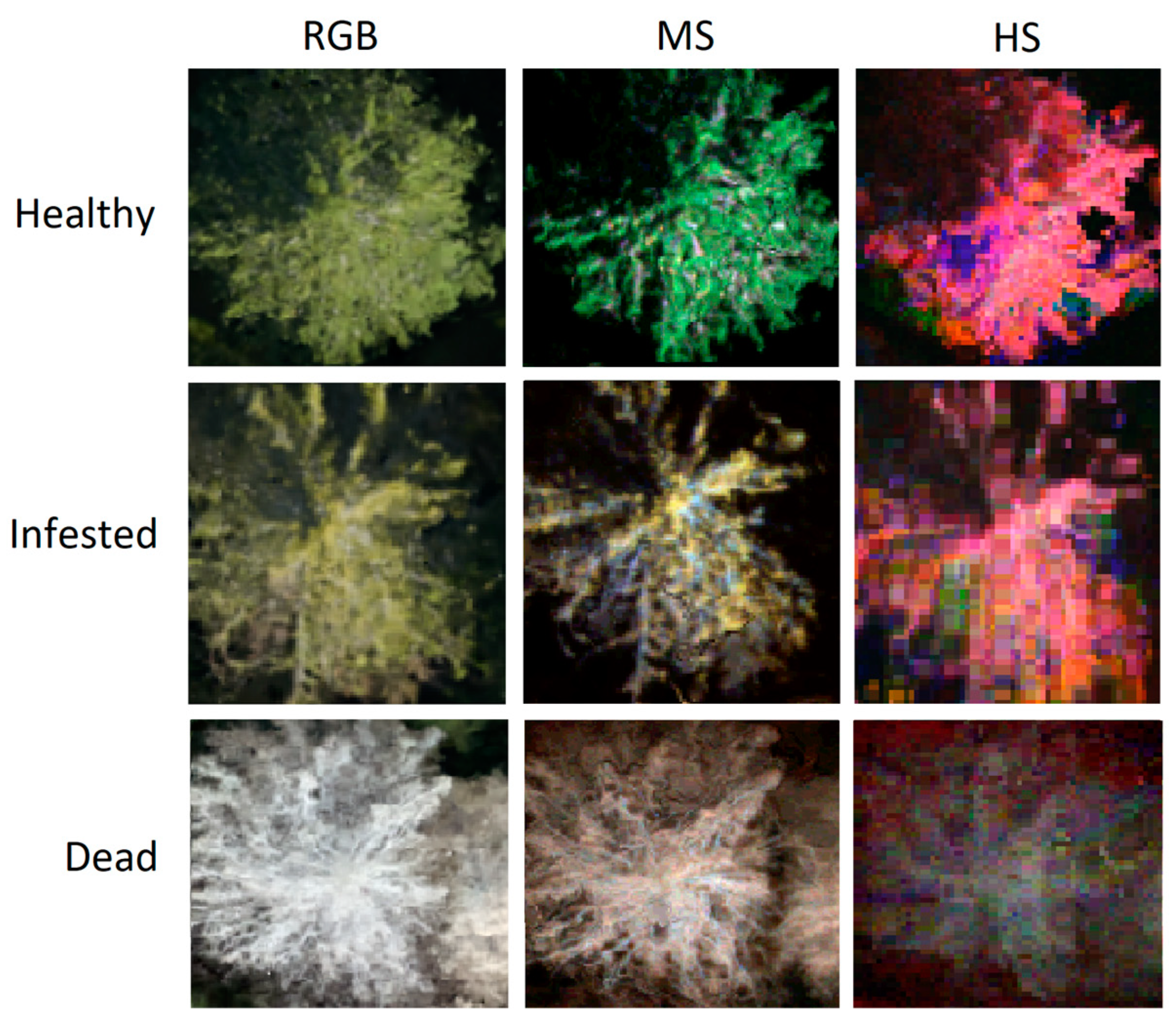
The methods for detecting bark beetle infestations from UAS images are usually based on crown discoloration symptoms that occur when the water and nutrient transportation of the tree are disturbed, and tree health begins to decline. The color of the crown gradually changes from green to yellow and finally to reddish brown and gray in the final step when the tree dies [9]. These color symptoms can be detected from UAS images taken of the tree crowns. A great challenge in the detection of bark beetle infestations is the identification of the early stages of infestation. The first visible signs of bark beetle infestations include entrance holes, thin resinous flows on the trunk of the tree, and boring dust below the entrance hole; however, these symptoms are challenging to detect from above the tree canopies [12]. Other trunk symptoms include bark flaking and shedding. The early stage of infestation when the first trunk symptoms are already visible but the crown is still green is referred to as the “green attack” phase [13].

Red–green–blue (RGB) [14,15] and multispectral (MS) cameras [13,16,17,18,19,20] have been the most frequently used technologies in recent UAS studies on forest insect pests and diseases. Hyperspectral (HS) cameras have been used in only a few studies from UAS [21,22] and manned platforms [9,21]. There is a need for using HS cameras characterized by a high radiometric resolution and a wide spectrum to enable a more rapid detection of infested trees [22].

A variety of computational approaches have been employed to detect tree stress from remote sensing images [18]. Thresholding spectral indices derived from different band combinations, such as the Normalized Difference Vegetation Index (NDVI) and Chlorophyll Vegetation Index (CVI), are a commonly used approach [9,13,16,23]. Other research efforts have employed machine learning algorithms, such as Random Forests (RFs) and Deep Neural Networks (DNNs), to classify healthy and stressed trees [14,15,19,20].

A study comparing three different convolutional neural network architectures and RFs for bark beetle symptom classifications from MS images showed that the CNNs outperformed RFs; the accuracies were 0.94 and 0.86 for infested and healthy spruces, respectively [19]. Studies using multitemporal MS images collected at early and later stages of bark beetle infestations showed that the classification of the different health stages was more accurate at the end of the summer season [16,20]. Recently, state-of-the-art single-stage DNN architectures You Only Look Once (YOLO) [24] and RGB images provided high accuracies in the detection and classification of infested trees. A mean average precision of 0.94 was obtained in a study conducted in Bulgaria [14], whereas the F-scores were 0.90, 0.79, and 0.98, respectively, for healthy, infested, and dead trees in a study conducted in Finland [15].

Despite the increasing research efforts, there is still a need for more precise and efficient methods to monitor forest health. RGB UAS imagery is not sufficient for the detection of the early infestation stage as the green attack trees cannot be detected from the visible crown discoloration symptoms [14]. For the early detection of bark beetle infestations, it may be advantageous to use MS and HS images that contain richer spectral information [11]. For example, the wavelength regions affected by leaf water content have been found to be sensitive to changes during the early stages of a bark beetle infestation [25]. MS and HS imaging can capture more spectral bands than RGB images with a higher spectral resolution. MS and HS capture wavelengths that have been shown to offer insights into cellular-level changes affecting plant health and can therefore be a useful tool for bark beetle infestation detection [26,27]. The limited use of advanced sensor technologies, such as HS cameras and LiDARs, has been considered a shortcoming in the present research, and it is expected that more detailed data would improve the performance of analytics [9,11,22]. Furthermore, the scientific literature lacks a thorough investigation of the performance of different DNN architectures in connection with different imaging techniques.

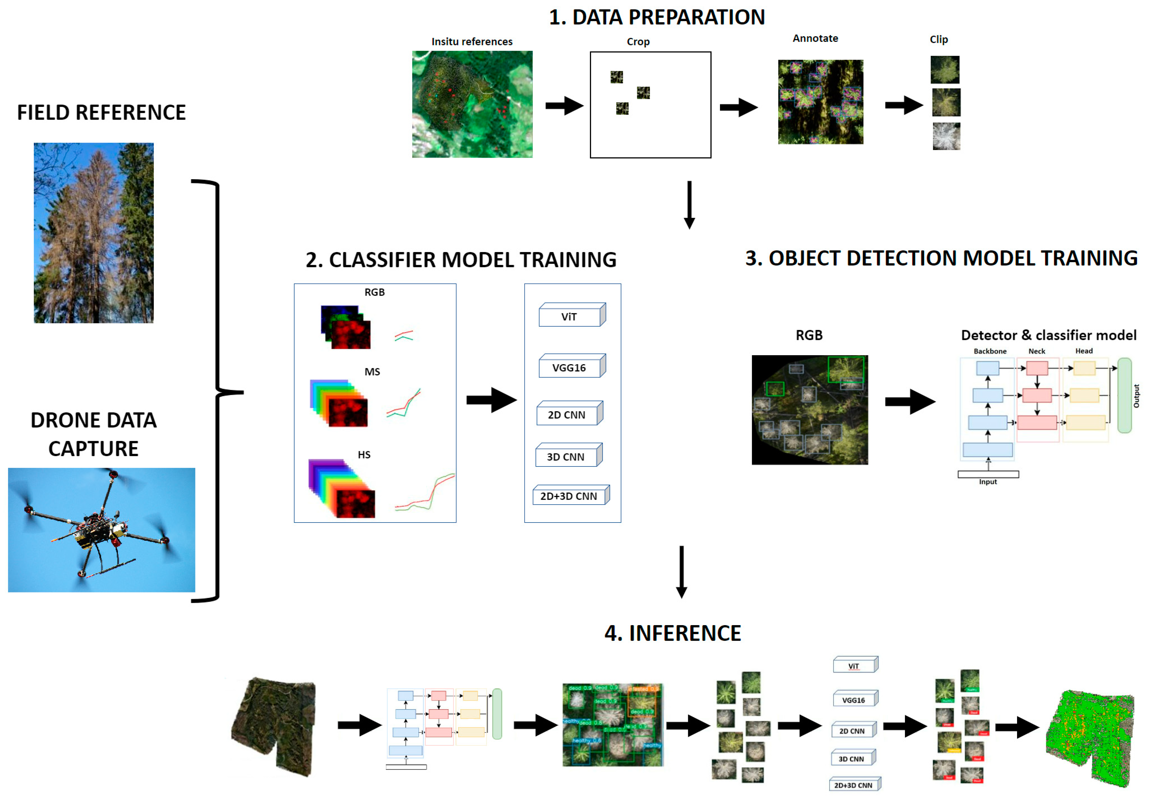
The overall objective of this study is to develop and assess deep learning-based methods for tree health analysis at individual tree levels utilizing high spatial and spectral resolution image data collected by a UAS. The study compares the effectiveness of different DNNs for identifying bark beetle damage on spruce trees using UAS RGB, MS, and HS images. The specific research questions aim to answer the following questions: (i) does the use of MS and HS images result in enhanced classification results compared to RGB images when using deep learning techniques? (ii) Which network structures work best for RGB, MS, and HS images? (iii) How does data augmentation impact the performance of the investigated classifiers? (iv) What kind of performance level is achieved by using single-stage detection and the classification network YOLO or integrating YOLO with a separate image classification network?

Our results highlight the potential of DNNs for the accurate and efficient detection of bark beetle damage and provide insights into the strengths and limitations of different network architectures for this task. The study also shows that careful consideration must be made to the data availability and model selection. Ultimately, this research has the potential to inform and improve the timely management of bark beetle infestations, contributing to more sustainable and resilient forest ecosystems.

2. Materials and Methods

2.1. Overview of the Method

We proposed to use a supervised machine learning approach to train DNN models to detect spruce trees and classify their health in different classes (Figure 1). The required input data were tree health references and UAS image datasets. Using these data, two kinds of neural networks were trained: classifier networks and single-stage object-detector and -classifier networks. Furthermore, these two approaches were cascaded to facilitate a combined and refined detection and classification workflow. The major phases of the method were data preparation, classifier model training, and object-detection model training. In the final stage, the cascaded object-detection and -classification models were used to perform inferences over large areas (Figure 1). In this study, we focused on implementing and assessing different models; however, we did not assess the full area inference model due to the lack of testing materials. Different steps of the proposed method are described in the following sections.

2.2. Study Areas and Reference Data

The UAS flights were conducted in Ruokolahti (61°29′21.840″N, 29°3′0.720″E), south Karelia, and the Paloheinä areas of Helsinki central park (60°15′25.200″N, 24°55′19.200″E) in southern Finland (Figure 2). The Ruokolahti area had four study areas, dominated by mature spruce stands: Murtomäki, Ryhmälehdonmäki, Paajasensalo, and Viitalampi. The Ruokolahti area was hit by a disastrous summer thunderstorm in 2010, felling trees in high numbers and a causing population explosion of the pest. Consequently, there was an outbreak of bark beetles in the area. Paajasensalo and Viitalampi are nature conservation areas. Spruce mortality and damage are more extensive in these two areas than in Murtomäki and Ryhmälehdonmäki, which are managed forests, and thus effective control measures target for them. The Helsinki central park area has been suffering from a bark beetle outbreak for a few years [20]. The main reasons for the outbreak are the favorable mature spruce-dominated forest stands as well as hot and dry summers, which have enabled the development of a second generation of bark beetles during a single summer and increased the bark beetle population at a calamitous level. All the study areas were in mature boreal forests dominated by Norway spruce trees with admixtures of Scots pine (Pinus sylvestris L.), Silver birch (Betula pendula L.), European aspen (Populus tremula L.), and rowan (Sorbus aucuparia L.).

The reference tree health data were collected during the fieldwork conducted by forest health specialists in the Ruokolahti and Paloheinä study areas. The Ruokolahti study areas were composed of 57 circular sampling plots with a 10 m radius, in which tree health status was analyzed. The center of each plot was located using a Trimble Geo XT GPS device (Trimble Navigation Ltd., Sunnyvale, CA, USA), and the individual trees were located by measuring the distance to and azimuth of each tree from the plot center. For each tree larger than 5 cm in diameter within a sampling plot, the tree species, diameter at breast height (dbh), and height (h) were recorded in August 2019. Additionally, for spruce trees, five symptoms indicating bark beetle infestation were recorded in August 2019 and 2020, including crown discoloration, defoliation, bark beetle entrance and exit holes in the trunk, resinous flow, and declined bark condition [8].

In the Paloheinä area, the health data for selected individual spruce trees distributed throughout the area were recorded, aiming to ensure a uniform distribution of different health statuses among the reference trees [20]. The positions of the trees were obtained from orthophotos collected before the tree selection. The data were collected in the spring, summer, and fall of 2020. Different trees were chosen for monitoring during each season. In total, 380 trees were monitored and the health symptoms recorded were crown color, defoliation, resinous flow, bark damage, and decreased vertical proportion of living canopy (compared to a healthy tree at the same site).

The labeling scheme classified trees into healthy, infested, or dead categories based on the crown color symptoms. Specifically, green and faded-green trees were labeled as healthy; yellow and yellowish trees as infested; while reddish/brown and gray trees were labeled as dead. The total numbers of the reference trees were 1466 for RGB images, 1242 for MS images, and 995 for HSI images (

Table 1. Total numbers of images assigned to each health class when using the crown color symptoms.

Area	Data Type	Total	Healthy	Infested	Dead
	RGB	604	231	162	211
Paloheinä	MS	380	141	109	130
	HS	502	208	130	164
	RGB	862	538	11	313
Ruokolahti	MS	862	538	11	313
	HS	493	307	3	183
	RGB	1466	769	173	524
Total	MS	1242	679	120	443
	HS	995	515	133	347

). The differences in the number of reference trees for different image datasets were the result of the differences in the data collection; the HS data had the smallest coverage. Most samples were of healthy and dead trees, while there were fewer samples from infested trees, especially in the Ruokolahti area.

2.3. Remote Sensing Datasets

In the Ruokolahti area, the UAS images were captured in August, in the years 2019 and 2020, except for Murtomäki, which only had data from 2019. During 2019, the data collection was conducted in blue-sky conditions; however, in 2020, the weather conditions varied (

Table 2. Instrument and acquisition details of the remote sensing datasets. FA: flying altitude; GSD: ground sample distance of the final orthomosaics; MM: Murtomäki, PS: Paajasensalo, RM: Ryhmälehdonmäki, VL: Viitalampi.

Dataset	Date	Area (ha)	Weather	FA (m)	GSD RGB; MS; HS (cm)	Equipment
MM_2019	28 August 2019	60	Sunny	140	3; 6; -	DualSonyA7RII, Altum
	14:08–14:32
	14:46–15:11
PS_2019	28 August 2019	45	Sunny	140	3; 6; -	DualSonyA7RII, Altum
	11:52–12:15
	12:27–12:51
PS_2020	27 August 2020	32	Varying	140	6; 6; -	SonyA7R, Altum
	16:30–17:00
RM_2019	27 September 2019	27	Sunny	140	6; 6; -	DualSonyA7RII, Altum
	13:05–13:27
	14:44–15:03	10	Sunny	140	-; -; 10	Rikola
RM_2020	27 August 2020	20	Sunny	140	4; 6; 10	DualSonyA7RII, Altum, Rikola
	10:05–10:27
VL_2019	27 August 2019	120	Sunny	140	6; 8; -	DualSonyA7RII, Altum
	16:11–16:34
	16:42–17:02
	28 August 2019
	9:26–9:47
	9:55–10:16
	29 August 2019	12	Sunny	140	-; -; 10	Rikola
	11:48–12:14
VL_2020	27 August 2020	25	Varying	140	6; 6; 10	DualSonyA7RII, Altum, Rikola
	11:26–11:50
	15:05–15:26	33	Varying	140	6; 6; -	SonyA7R, Altum
PH_2020_1	20 May 2020	24	Varying	110	5; 5; -	Sony A7R, Altum
	12:18–12:39
PH_2020_2	15 July 2020	24	Sunny	110	5; 5; 10	DualSonyA7RII, Altum, Rikola
	10:41–11:04
	11 September 2020	24	Cloudy	110	5; 5; 10	DualSonyA7RII, Altum, Rikola
	11:16–11:40
PH_2020_3	23 September 2020	24	Varying	110	5; -; 10	DualSonyA7RII, Rikola
	10:08–10:32

). The Paloheinä datasets obtained captured in the spring, summer, and fall of 2020. The sizes of individual study areas were 20–120 ha, and the total area was 252 ha in 2019 and 152 ha in 2020 (Table 2). The study areas were captured in 1–4 separate flights, depending on the size of the area. A custom-built quadcopter UAS with a Gryphon Dynamics frame (Gryphon Dynamics Co., Ltd., Daegu, Republic of Korea) was used in all campaigns (Figure 3).

The RGB images were captured using Sony A7R and Sony A7R II full-frame cameras (Sony Group Corporation, Tokyo, Japan). The MS images were captured with a Micasense Altum (AgEagle Aerial Systems Inc., Wichita, KS, USA) camera, of which five visible and near-infrared (VNIR) channels were used in this study. HS images were collected with a Rikola camera (Senop Ltd., Oulu, Finland), which captured 46 spectral channels in the range of 500–900 nm, with a Full-Width of Half Maximum (FWHM) of 6.36–10.16 nm (average 6.9 nm) and a spectral resolution (distance between adjacent bands) between 4.87–14.94 nm (average of 8.98 nm). To enable georeferencing, a Trimble’s APX-15 EI UAV GNSS-Inertial OEM positioning system consisting of a multiband GNSS, an Inertial Measurement Unit (IMU), and a Harxon HX-CHX600A Antenna (Harxon Corporation, Shenzhen, China) was integrated into the system. Figure 3 shows the UAS setup used in 2019 with the HS and dual RGB cameras; in this photo, Micasense RedEdge is used instead of Altum. The central wavelengths (L0) and bandwidths (FWHM) of each spectral band of the Micasense Altum and Rikola cameras are presented in

Table 3. Spectral camera settings for multispectral and hyperspectral cameras. L0: central wavelength; FWHM: full-width of half maximum.

Quantity	Values
Micasense Altum L0 (nm)	475, 560, 668, 717, 840, 12,000
Micasense Altum FWHM (nm)	20, 20, 10, 10, 40, 6000
Rikola L0 (nm)	504.28, 512.91, 521.48, 530.75, 539.46, 548.45, 557.59, 566.28, 575.31, 583.98, 593.37, 601.4, 611.64, 620.27, 628.86, 643.8, 648.67, 657.82, 666.88, 676.21, 684.56, 693.97, 701.6, 711.43, 720.08, 728.95, 738.01, 746.76, 756.03, 764.56, 773.71, 782.85, 792.18, 800.88, 809.82, 818.49, 828.84, 837.57, 846.22, 855.44, 863.54, 873.07, 881.51, 890.21, 899.16, 908.17
Rikola FWHM (nm)	6.36, 7.26, 7.47, 6.75, 7.42, 6.64, 7.35, 6.47, 7.02, 6.6, 6.18, 6.49, 7.64, 8.3, 7.05, 6.76, 6.58, 7.58, 6.72, 7.52, 6.66, 6.82, 5.01, 4.43, 4.97, 3.92, 4.86, 4.11, 4.49, 3.67, 4.3, 5.95, 5.8, 6.46, 5.67, 6.62, 9.05, 10.16, 9.24, 9.93, 9.46, 9.21, 9.55, 9.03, 9.58, 8.9

.

The raw images underwent geometric and radiometric corrections to provide georeferenced orthomosaics and to eliminate external disturbances caused by the sensor, atmosphere, and weather conditions. The processing of RGB and MS was conducting using Agisoft PhotoScan 1.4.3 (Agisoft LLC, St. Petersburg, Russia). For the HS images, the georeferencing of reference bands was performed using Agisoft PhotoScan 1.4.3, followed by band matching and orthomosaic calculations using in-house software [28,29]. The Ground Sample Distance (GSD) values of the final orthomosaics were 0.03 to 0.06 m for RGB datasets, 0.05 to 0.08 m for MS datasets, and 0.10 m for HS datasets.

2.4. Data Preparation

The data preparation included individual tree crown extraction and the labeling of datasets for object-detection networks.

For the object-detection task, the RGB orthophotos captured in the research areas were cropped to cover only the sub-areas that contained the reference trees selected for tree health monitoring. To optimize the detection algorithm’s performance, the large sub-areas of monitored trees were divided into smaller sections. The dimensions of the resulting images varied, with width and height ranging from 300 to 1000 pixels. The cropped sections comprised both labeled and unlabeled trees (Figure 4a). Unlabeled trees were removed from the images to prevent them from being learned as negative samples. Since there was no recorded information for the locations of unlabeled trees, they were manually removed from the images via a visual inspection (Figure 4b). These types of images were used as the input for the YOLO detection network. As the YOLO network was not designed to process MS and HS images, the detection and classification were performed on RGB images.

To create the input images for the classifier networks, each reference tree crown was cropped from the images based on its bounding box coordinates. For the RGB datasets with the highest spatial resolutions, all tree crown images were resampled to uniform square shapes of 150 × 150 pixels using nearest-neighbor resampling. The MS and HS datasets were resampled to 100 × 100 pixels and 50 × 50 pixels, respectively. Notably, an exception was made for the VGG16 and ViT networks, where all the images were resized to 224 × 224 pixels. The resulting input image to the classifier networks was a data cube of a w × h × d shape, where w and h represented the pixel width and height of the image, respectively, and d represented the number of channels in the image. Figure 5 shows examples of cropped tree crown images and depicts the appearance of the healthy, infested, and dead classes on RGB, MS, and HS images.

The reference datasets were divided into training, validation, and independent test sets. The test set was chosen by manually selecting two study areas as the test data. The selection criteria for the test set were established based on multiple factors. Firstly, it was deemed essential for the test set to comprise a significant number of images that adequately represented all health classes. Moreover, the test set needed to be suitable for conducting tests on the RGB, multispectral, and hyperspectral images. Consequently, Viitalampi 2020 and Paloheinä 15 July 2020 datasets were identified as suitable candidates for the test data. These specific datasets were selected due to their availability across all image types and their ability to provide a satisfactory number of infested trees, thus meeting the desired number required for a comprehensive analysis. The remaining data were divided into training and validation sets using a random shuffle, adhering to an 80:20 split.

2.5. Classifier Model Training

2.5.1. Classifier Networks

The networks used were based on several research papers in the remote sensing field, mainly used for tree species and health classifications [30,31,32,33,34,35,36]. The used networks included VGG16, ViT, a simple 2D-CNN, and several 3D- and 2D-3D-CNNs. The different networks, their layers, and numbers of trainable parameters are summarized in

Table 4. CNN architectures and numbers of trainable parameters in each network model. FC: fully connected layer; BN: batch normalization.

Network	Layers	Number of Kernels and Kernel Sizes	Number of Trainable Parameters
VGG16	2 × Conv2D–MaxPool–	(64) 3 × 3	~134 million
	2 × Conv2D–MaxPool–	(128) 3 × 3
	3 × Conv2D–MaxPool–	(256) 3 × 3
	3 × Conv2D–MaxPool–	(512) 3 × 3
	3 × Conv2D–MaxPool–	(512) 3 × 3
	3 × FC
2D-CNN	Conv2D–BN–MaxPool–	(32) 3 × 3	~200,000
	Conv2D–BN–MaxPool–	(64) 3 × 3
	Conv2D–BN–AvgPool–	(64) 3 × 3
	FC–Dropout–FC
3D-CNN 1	Conv3D–MaxPool–	(32) 3 × 3 × 3	~300,000
	Conv3D–MaxPool–	(64) 3 × 3 × 3
	Conv3D–AvgPool–	(64) 3 × 3 × 3
	FC–Dropout–FC
3D-CNN 2	Conv3D–MaxPool–	(20) 5 × 5 × 5	~100,000
	Conv3D–MaxPool–	(50) 5 × 5 × 5
	Conv3D–	(3) 1 × 1 × 1
	FC–FC
3D-CNN 3	Conv3D–MaxPool–	(5) 3 × 3 × 3	~387 million
	Conv3D–MaxPool–	(10) 3 × 3 × 3
	Conv3D–MaxPool–	(15) 3 × 3 × 3
	FC–FC
3D-CNN 4	Conv3D–	(4) 3 × 3 × 7	~236 million
	Conv3D–	(8) 3 × 3 × 7
	Conv3D–	(16) 3 × 3 × 7
	Conv3D–	(32) 3 × 3 × 7
	Conv3D–MaxPool–	(64) 3 × 3 × 7
	Dropout–FC–Dropout–FC
2D-3D-CNN 1	Conv2D–	(46) 3 × 3	~13 million
	Conv3D–MaxPool–	(200) 3 × 3 × 3
	2D-Deconvolution–	(1) 3 × 3
	FC–FC
2D-3D-CNN 2	Branch 1:		~23 million
	Conv3D–	(1) 7 × 7 × 7
	Conv2D	(6 ∗ 46) 3 × 3
	Branch 2:
	Conv3D–	(1) 5 × 5 × 5
	Conv3D–	(6) 3 × 3 × 3
	Conv2D	(12 ∗ 46) 3 × 3
	Branch 3:
	Conv3D–	(1) 3 × 3 × 3
	Conv3D–	(8) 3 × 3 × 3
	Conv3D–	(12) 3 × 3 × 3
	Conv2D	(32 ∗ 46) 3 × 3
	Concatenation
	FC–FC–FC–FC
2D-3D-CNN 3	Feature extractor:		~10 million
	Conv3D–BN–	(1) 3 × 3 × 5
	Conv3D–BN	(8) 3 × 3 × 5
	Conv3D–BN–	(16) 3 × 3 × 5
	Conv3D–BN	(24) 3 × 3 × 5
	Spatial encoder:
	Conv2D–	(32 ∗ 46) 3 ×
	Conv2D–BN–	(32 )3 × 3
	Conv2D–	(16) 3 × 3
	Conv2D–BN–	(16) 3 × 3
	FC

for the CNNs and

Table 5. ViT architecture and number of trainable parameters.

Network	Layers	Number of Trainable Parameters
ViT	Transformer encoder	~22 million
	12 × (Layer norm–MHA block–Skip connection–
	Layer norm–FC block–Skip connection)

for ViT. All the models were trained from scratch, such that the initial weights were chosen at random.

VGG16 is a CNN architecture that was developed by the Visual Geometry Group (VGG) at the University of Oxford [37]. It consists of 16 layers, including 13 convolutional and 3 fully connected layers. The input to the network is a 224 × 224 image. Max pooling layers follow convolution blocks, as described in Table 4. The final layer of the network is a SoftMax layer that produces a probability distribution over the possible classes. The VGG16 architecture has achieved state-of-the-art results on many computer vision tasks, including the ImageNet Large Scale Visual Recognition Challenge (ILSVRC) in 2014. The used model was VGG-16-BN, which was downloaded from the Pytorch torchvision library.

The employed 2D-CNN architecture [30] comprised three consecutive convolutional layers, each sequentially accompanied by a batch normalization layer and activated using the ReLU function. Subsequent to the initial two convolutional layers, max pooling was applied, while average pooling was employed after the final convolutional layer, enhancing the network’s feature extraction. The convolution blocks were followed by two fully connected layers with ReLU activation, and the first connected layer was followed by a dropout layer.

To evaluate the efficacy of 3D convolutions in the HS-image feature extraction, a comparison was made between 3D-CNNs and the 2D-CNN network. The 3D-CNNs were implemented based on four initial models described in research papers in the field [30,31,32,33]. In addition, three 2D-3D-CNNs were also implemented based on the literature [34,35,36].

The 3D-CNN 1 [30] exhibited resemblances to the 2D-CNN introduced in the same study. However, the 2D-convolution layers were transformed into 3D convolutions, while the batch normalization process was omitted. Retaining consistency, the remaining network layers mirrored those of the 2D-CNN, including the quantities of kernels and kernel sizes implemented.

The 3D-CNN 2 [31] featured three convolutional layers. Following the initial two convolutional layers, the design incorporated max pooling, succeeded by ReLU activation after the second pooling layer, just prior to the ultimate convolutional layer. Furthermore, the model incorporated two fully connected layers into its configuration.

The 3D-CNN 3 [32] resembled the 3D-CNN 2 in structure, both encompassing three convolutional layers and incorporating max pooling. Nevertheless, in contrast to the 3D-CNN 2, each convolutional layer in the 3D-CNN 3 was accompanied by ReLU activation, followed by max pooling. Additionally, the model integrated a pair of fully connected layers into its configuration.

3D-CNN 4 [33], the deepest of the employed 3D-CNNs, showcased an architecture featuring five convolutional layers. After each convolutional layer, ReLU activation was incorporated, while max pooling was executed subsequent to the final convolution and its accompanying ReLU activation. Additionally, the model included two fully connected layers, preceded by dropout layers.

The utilized 2D-3D-CNNs consisted of alternating layers of 2D and 3D convolutions. The first network, denoted here as 2D-3D-CNN 1 [34], comprised a 2D-convolution layer followed by a 3D-convolution layer and then by a max pooling layer and ReLU activation. Subsequently, a 2D deconvolution was applied, followed by two fully connected layers.

2D-3D-CNN 2 [35] consisted of three branches of convolutions. The first branch contained one 3D-convolution layer, the second branch two 3D-convolution layers, and the third contained three 3D-convolution layers. ReLU activation followed all 3D convolutions, and each branch contained a single 2D-convolution layer. The outputs from all branches were concatenated and passed through four fully connected layers.

2D-3D-CNN 3 [36] incorporated feature extractor and spatial encoder modules. The feature extractor module was composed of four 3D-convolution layers, each followed by a batch normalization layer and ReLU activation. The output of each convolution layer was concatenated to create a stack of output data cubes. On the other hand, the spatial encoder module transformed a 3D input into an encoded feature vector representation using separable 2D convolutions, followed by a batch normalization layer and ReLU activation. Finally, a fully connected layer was placed at the end of the network to produce the output feature vector. It is worth noting that the feature extractor module was based on 3D convolutions, while the spatial encoder module employed 2D convolutions.

Vision Transformer (ViT) [38] is a transformer network designed for image classification tasks (Table 5). The transformer-based architecture of ViT processes the image patches as a sequence of tokens. The input to the network is a fixed-size image, which is split into a grid of non-overlapping patches. These patches are then flattened into a sequence of tokens and fed into a transformer encoder. The transformer consists of multiple layers of self-attention and feed-forward networks, which learn to model the interactions between the image patches. The output of the transformer is then fed into a classification head that produces a probability distribution over the possible classes. ViT has achieved state-of-the-art results on many image classification tasks, including the ImageNet dataset [39]. The used ViT version was ViT-S, with 16 patches and an image size of 224 × 224 pixels. The model was downloaded from the Pytorch image models library, timm.

The hyperparameters used in the training stages for each network were selected with the Optuna [40] hyperparameter optimization framework, as described in Section 2.5.2. Each model was trained for 500 epochs.

2.5.2. Hyperparameter Optimization

The Optuna framework [40] was used to optimize model training and improve the generalization ability of the models. The framework optimized an objective function, which, in this study, aimed to maximize the mean F1-score of the model when evaluated on the validation set (see description of F1-score in Section 2.8). Maximizing the mean F1-score across all classes is a reasonable goal for achieving a good overall performance. The parameters to optimize were the initial learning rate, weight decay, and batch size. Default values were used for the rest of the parameters. The optimal parameter values found with this method are presented in

Table 6. Optimized hyperparameter values for each model.

Network	Data	Learning Rate	Weight Decay	Batch Size
VGG16	RGB	0.000005	0.02	12
ViT	RGB	0.000001	0.05	32
2D-CNN	RGB	0.00002	0.02	12
VGG16	MS	0.000001	0.03	32
ViT	MS	0.000001	0.02	48
2D-CNN	MS	0.0001	0.08	32
VGG16	HS	0.0000005	0.03	12
ViT	HS	0.0000003	0.06	32
2D-CNN	HS	0.000005	0.04	12
3D-CNN 1	HS	0.000004	0.01	32
3D-CNN 2	HS	0.000005	0.02	32
3D-CNN 3	HS	0.00001	0.01	32
3D-CNN 4	HS	0.00003	0.04	32
2D-3D-CNN 1	HS	0.00002	0.04	32
2D-3D-CNN 2	HS	0.00002	0.03	24
2D-3D-CNN 3	HS	0.00001	0.02	12

.

The default sampling algorithm, the tree structured Parzen estimator TPESampler, was used, as recommended in a previous study [41], for an optimization with limited parallel computing resources. TPESampler uses an iterative process that utilizes the history of already-evaluated hyperparameter values to create a probabilistic model that suggests new hyperparameter values to optimize the target function. The iteration continues until a specified number of trials are performed. In this study, we set the number of initial random selections as 10, after which the algorithm started to use the Parzen model estimation to suggest new values. We use 200 trials as TPE requires many iterations to converge to an optimal solution, and it is recommended to run it for at least 200 iterations.

To reduce the time taken to reach the optimal solution, we used pruning algorithms that could be used to automatically stop un-promising trials at the early stages of the training stage. This reduced the time taken to reach the optimal solution as trials likely to achieve poor results were pruned out. We use the HyperbandPruner algorithm, which takes advantage of the asynchronous successive halving algorithm [42] by using multiple successive halving pruners that are referred to as brackets. Each bracket observes multiple trials and prunes out the worst trials in the bracket. The number of brackets is determined by the parameters min_resource, max_resource, and reduction_factor. The max_resource parameter should be set to the number of epochs used in the training, and min_resource controls the sensitivity of the pruning behavior. A smaller min_resource leads to faster run times; however, a higher min_resource achieves more reliable results as it provides a better guarantee of successful judging between the trials. The reduction_factor parameter specifies the fraction of trials to be reduced. In this study, we set the max_resource value to 500, according to the number of training epochs, and min_resource to three to increase its value from the default of one but kept the number of brackets as four. The reduction_factor was kept as the default, which was three.

2.5.3. Data Augmentation

The dataset used in this study displayed an imbalanced distribution of object classes, with a significantly higher proportion of healthy trees in comparison to those classified as infested and dead. Specifically, the proportion of healthy trees was approximately four-times greater than that of infested trees and 50% larger than the proportion of dead trees. This imbalance in the distribution of classes could lead to a biased training of the network due to the overwhelming number of healthy trees in the dataset.

To counter this issue, data augmentation was employed to increase the number of infested and dead tree samples in the training dataset. Three copies were created for each infested tree image, and one copy was created for half of the dead tree images. These duplicated images were then subjected to various augmentation techniques.

To determine the optimal augmentation procedure, a selection of transforms from PyTorch’s torchvision [43] transforms library was tested. Initially, all transforms were applied to the images and, subsequently, each transform was excluded in subsequent trials to identify any transforms that positively impacted the results. The evaluation criterion focused on the F1-score of infested trees, emphasizing the augmentation strategy’s specific aim to improve the classification results for this category. The augmentations were tested using different models: VGG16 for RGB images, 2D-CNN for MS images, and 2D-3D-CNN 2 for HS images.

The selection of transforms included random rotation [44], the horizontal and vertical flipping of images [45,46], Gaussian blurring [47], padding [48], and random perspective shifts [49]. In the random rotation transform, each augmented image was rotated by a random degree within the range of [–180, 180], padding added whitespace to the sides of the image, effectively reducing its size. Random perspective shifts altered the image perspective by a random distortion factor, while Gaussian blur applied a randomly selected Gaussian blur to the image.

2.6. YOLO Implementation

The single-stage object-detection and -classifier framework YOLOv4-p5 [50] was used to implement the entire tree-detection and -classification procedure. A similar setup was used, as in reference [15] (

Table 7. YOLO architecture and number of trainable parameters. *: Layers inside brackets are repeated four times; **: Layer is repeater five times.

Network	Layers	Number of Kernels and Kernel Sizes	Number of Trainable Parameters
YOLO	Conv2D–MaxPool–	(64) 7 × 7	~64 million
	Conv2D–MaxPool–	(192) 3 × 3
	Conv2D–	(128) 1 × 1
	Conv2D–	(256) 3 × 3
	Conv2D–	(256) 1 × 1
	Conv2D–MaxPool–	(512) 3 × 3
	4 × (Conv2D–	(256) 1 × 1
	Conv2D–) *	(512) 3 × 3
	Conv2D–	(512) 1 × 1
	Conv2D–MaxPool–	(1024) 3 × 3
	Conv2D–	(512) 1 × 1
	Conv2D–	(1024) 3 × 3
	Conv2D–	(512) 1 × 1
	5 × Conv2D– **	(1024) 3 × 3
	FC–FC

). In this study, the spruces identified by YOLO were fed into the classifier networks to compare their performances to YOLO.

The YOLOv4 architecture is built on a strong backbone, namely, CSPDarknet53 [51], which leverages cross-spatial partial connections. This architectural design effectively splits the feature map of the base layer into two branches, one passing through convolution layers and the other bypassing convolutions, facilitating an improved gradient flow. The neck component, comprising modified spatial pyramid pooling and a path aggregation module, enhanced feature representation and information fusion processes. Finally, the dense predictor block (head) employed multiple prediction layers with anchor boxes to locate bounding boxes and predict object classes. YOLOv4 uses several approaches to enhance accuracy and address the challenges in object detection. Data augmentation techniques, such as mosaic data augmentation and random anchor shapes, were employed to augment the training data diversity and improve model robustness. The anchor boxes were optimized using the K-means clustering algorithm to align with the distribution of object sizes, enabling a better localization.

A YOLOv4-p5 model, initially pretrained on the COCO [52] 2017 object-detection dataset, was utilized and subsequently fine-tuned with the RGB dataset. The fine-tuning process involved training the model for 200 epochs, employing default hyperparameter values.

2.7. Computing Platform

Each classifier network model was trained using a NVIDIA Quadro RTX 6000 Graphics Processing Unit (GPU) with 24 GB of memory. The durations of the training sessions ranged from 15 min to approximately 3 hours, depending on the complexity of the models and used data. For the YOLO object-detector network, training was performed on a NVIDIA GeForce GTX 1080 Ti GPU equipped with 11 GB of memory (

Table 8. Training time for each model on the used datasets.

Model	Training Time (min)
	RGB	MS	HS
VGG16	135	128	157
2D-CNN	16	15	17
3D-CNN 1	-	-	48
3D-CNN 2	-	-	36
3D-CNN 3	-	-	173
3D-CNN 4	-	-	189
2D-3D-CNN 1	-	-	62
2D-3D-CNN 2	-	-	128
2D-3D-CNN 3	-	-	115
ViT	144	139	168
YOLO	144	-	-

).

2.8. Evaluation Metrics

The performances of the trained models were evaluated on independent test sets containing data not used in the training. The evaluation metrics employed in the study were class-wise precision (1) and recall (2) scores, along with their harmonic means, F1-scores (3) [53]. Additionally, the overall accuracy was calculated.

Precision measures the specificity of a model as the ratio of true positive (TP) predictions to the sum of true positive and false positive (FP) predictions. The formula for precision can be mathematically represented as:

$$\mathrm{p}\mathrm{r}\mathrm{e}\mathrm{c}\mathrm{i}\mathrm{s}\mathrm{i}\mathrm{o}\mathrm{n}=\frac{\mathrm{T}\mathrm{P}}{\mathrm{T}\mathrm{P}+\mathrm{F}\mathrm{P}}$$

(1)

Recall is a metric that quantifies the sensitivity of a model as the ratio of true positive predictions to the sum of true positive and false negative predictions. The mathematical formula for recall can be represented as:

$$\mathrm{r}\mathrm{e}\mathrm{c}\mathrm{a}\mathrm{l}\mathrm{l}=\frac{\mathrm{T}\mathrm{P}}{\mathrm{T}\mathrm{P}+\mathrm{F}\mathrm{N}}$$

(2)

Precision and recall are inversely related metrics. As the precision increases, the recall tends to decrease, and vice versa. Achieving high precision and recall scores simultaneously is a desirable element of a model’s performance, and the F1-score provides a measure of the optimal balance between these two metrics. The F1-score is calculated as the harmonic mean values of precision and recall. The mathematical formula for the F1-score can be represented as:

$${\mathrm{F}}_1=2·\frac{\mathrm{p}\mathrm{r}\mathrm{e}\mathrm{c}\mathrm{i}\mathrm{s}\mathrm{i}\mathrm{o}\mathrm{n}·\mathrm{r}\mathrm{e}\mathrm{c}\mathrm{a}\mathrm{l}\mathrm{l}}{\mathrm{p}\mathrm{r}\mathrm{e}\mathrm{c}\mathrm{i}\mathrm{s}\mathrm{i}\mathrm{o}\mathrm{n}+\mathrm{r}\mathrm{e}\mathrm{c}\mathrm{a}\mathrm{l}\mathrm{l}}$$

(3)

The overall accuracy provides the proportion of correct classifications out of the total number of classifications made. However, the overall accuracy may not always be the best metric to use, especially if the dataset is imbalanced or if certain classes are more important than others. Hence, class-wise evaluation metrics are crucial for evaluating the model performance with regard to the infested class predictions when the proportion of the infested tree samples is small.

3. Results

3.1. Classification Results

Overall, different datasets and classifiers provided relatively high and even classification accuracies for the healthy and dead spruce classes, while the accuracies were poorer for the infested class (

Table 9. Classification results of networks trained on unaugmented RGB, MS, and HS images. Numbers of reference trees in the training (Tr), validation (Va), and test (Te) sets are also given.

Model	Data	Overall Accuracy	Class	Precision	Recall	F1-Score	N-Reference Tr; Va; Te
VGG16	RGB	0.813	Healthy	0.776	0.894	0.831	524; 131; 114
			Infested	0.800	0.466	0.589	118; 29; 26
			Dead	0.816	1.000	0.899	374; 93; 57
ViT	RGB	0.815	Healthy	0.780	0.889	0.831	524; 131; 114
			Infested	0.598	0.406	0.484	118; 29; 26
			Dead	0.958	1.000	0.979	374; 93; 57
2D-CNN	RGB	0.789	Healthy	0.712	0.883	0.788	524; 131; 114
			Infested	0.582	0.561	0.571	118; 29; 26
			Dead	0.941	0.972	0.956	374; 93; 57
VGG16	MS	0.867	Healthy	0.935	0.864	0.898	452; 113; 114
			Infested	0.528	0.865	0.656	75; 19; 26
			Dead	0.943	0.978	0.960	309; 77; 57
ViT	MS	0.800	Healthy	0.877	0.655	0.750	452; 113; 114
			Infested	0.585	0.699	0.637	75; 19; 26
			Dead	0.893	0.988	0.938	309; 77; 57
2D-CNN	MS	0.901	Healthy	0.946	0.879	0.911	452; 113; 114
			Infested	0.765	0.684	0.722	75; 19; 26
			Dead	0.825	0.979	0.895	309; 77; 57
VGG16	HS	0.758	Healthy	0.972	0.589	0.734	321; 80; 114
			Infested	0.531	0.699	0.604	86; 21; 26
			Dead	0.901	0.988	0.942	232; 58; 57
ViT	HS	0.827	Healthy	0.872	0.797	0.833	321; 80; 114
			Infested	0.673	0.437	0.530	86; 21; 26
			Dead	0.899	1.000	0.947	232; 58; 57
2D-CNN	HS	0.801	Healthy	0.887	0.717	0.793	321; 80; 114
			Infested	0.588	0.476	0.526	86; 21; 26
			Dead	0.796	0.915	0.851	232; 58; 57
3D-CNN 1	HS	0.866	Healthy	0.896	0.859	0.877	321; 80; 114
			Infested	0.597	0.648	0.621	86; 21; 26
			Dead	0.901	0.968	0.933	232; 58; 57
3D-CNN 2	HS	0.807	Healthy	0.866	0.762	0.811	321; 80; 114
			Infested	0.539	0.788	0.640	86; 21; 26
			Dead	0.958	0.962	0.960	232; 58; 57
3D-CNN 3	HS	0.859	Healthy	0.776	0.976	0.864	321; 80; 114
			Infested	0.577	0.811	0.674	86; 21; 26
			Dead	0.912	0.988	0.948	232; 58; 57
3D-CNN 4	HS	0.847	Healthy	0.768	0.955	0.851	321; 80; 114
			Infested	0.564	0.846	0.677	86; 21; 26
			Dead	0.882	0.968	0.952	232; 58; 57
2D-3D-CNN 1	HS	0.833	Healthy	0.855	0.900	0.877	321; 80; 114
			Infested	0.596	0.423	0.495	86; 21; 26
			Dead	0.889	0.971	0.928	232; 58; 57
2D-3D-CNN 2	HS	0.829	Healthy	0.893	0.742	0.809	321; 80; 114
			Infested	0.626	0.911	0.742	86; 21; 26
			Dead	0.938	0.968	0.952	232; 58; 57
2D-3D-CNN 3	HS	0.755	Healthy	0.848	0.797	0.822	321; 80; 114
			Infested	0.542	0.393	0.456	86; 21; 26
			Dead	0.845	0.933	0.887	232; 58; 57

). The healthy-class F1-scores were 0.76–0.90 and, on average, 0.82. Correspondingly, the F1-scores were 0.85–0.98 and, on average 0.93, for the dead class. The infested-class F1-scores were 0.46–0.74 and had an average of 0.60.

When comparing the F1-scores of the infested class using different RGB and MS models, VGG16 and 2D-CNN outperformed the ViT model, despite ViT achieving a slightly higher overall accuracy than VGG16 and 2D-CNN for the RGB images. The good overall accuracy can be attributed to its effective classification of healthy and dead trees. However, the VGG16 and 2D-CNN models demonstrated better F1-scores when dealing with the infested class. VGG16 provided the best classification results with the RGB data, and 2D-CNN provided the best classification results with the MS-data for the infested class. However, among all the models and datasets (MS and HS), the ViT model trained on the RGB dataset yielded the best results for the dead class, achieving an F1-score of 0.98.

For the HS dataset, 3D-CNN 3 and 4 produced 5–8% better F1-scores for the infested class than the 3D-CNN 1 and 2 models. All HS 3D-CNN models outperformed the HS VGG16, ViT, and 2D-CNN models. The HS 2D-3D CNN 2 model provided the best results for the infested class, with an F1-score of 0.742. The 2D-3D CNN 1 and 3 models produced the poorest performances for the infested class of all HS models.

The best F1-scores for the infested class were 0.589, 0.722, and 0.742, for RGB, MSI, and HS models, respectively; thus, the HS models provided the best classification performance for the infested trees. The overall accuracies were 0.813, 0.901, and 0.829, respectively, for the corresponding models. The MS models thus provided a better overall accuracy than the HS models. This was due to the better results of the healthy trees in the MS models; the healthy class dominated the accuracy results due to the larger number of test samples in the healthy test data.

3.2. Impact of Data Augmentation

Through the analysis of the impact of different augmentations, the study identified the optimal data augmentation method, which comprised the utilization of random rotation, padding, and random perspective shift transforms. These selected transforms demonstrated the greatest potential for enhancing the performance of the model and were deemed crucial components of the augmentation process.

The best classifier models were all trained on the augmented dataset. Data augmentation improved the results in most cases (

Table 10. Classification results of models trained on augmented data. In column “Relative F1-score change”, positive values indicate an improvement. OA: overall accuracy.

Model	Data	OA	Class	Prec.	Recall	F1-Score	Relative F1-Score Change (%)	N-reference Tr; Va; Te
VGG16	RGB	0.848	Healthy	0.882	0.851	0.866	4.04	524; 131; 114
			Infested	0.722	0.500	0.591	0.34	588; 147; 26
			Dead	0.826	1.000	0.905	0.66	570; 142; 57
2D-CNN	RGB	0.821	Healthy	0.773	0.855	0.812	2.96	524; 131; 114
			Infested	0.577	0.601	0.589	3.06	588; 147; 26
			Dead	0.954	0.976	0.965	0.93	570; 142; 57
2D-CNN	MS	0.858	Healthy	0.898	0.851	0.874	−4.23	452; 113; 114
			Infested	0.739	0.654	0.694	−4.03	360; 90; 26
			Dead	0.833	0.965	0.894	−0.11	370; 92; 57
3D-CNN 3	HS	0.861	Healthy	0.813	0.924	0.865	0.12	321; 80; 114
			Infested	0.619	0.811	0.702	3.99	428; 107; 26
			Dead	0.945	0.978	0.961	1.56	297; 74; 57
3D-CNN 4	HS	0.863	Healthy	0.789	0.945	0.860	1.05	321; 80; 114
			Infested	0.597	0.855	0.703	3.70	428; 107; 26
			Dead	0.913	0.988	0.949	−0.32	297; 74; 57
2D-3D-CNN 2	HS	0.863	Healthy	0.968	0.807	0.880	8.07	321; 80; 114
			Infested	0.688	0.846	0.759	2.24	428; 107; 26
			Dead	0.880	0.982	0.928	−2.59	297; 74; 57

). The greatest improvements of 2.0–4.0% were obtained for the infested class with the RGB and HS models. In the case of MS models, the data augmentation reduced the F1-scores by approx. 4.0% for the healthy and infested classes, while the dead-class F1-score stayed practically the same.

The confusion matrix of the best-performing models showed that the greatest misclassification appeared between the healthy and infested trees (

Table 11. Confusion matrices of the best-performing RGB, MS, and HS models.

				Measured
			Healthy	Infested	Dead
VGG16 RGB	Predicted	Healthy	97	13	0
		Infested	5	13	0
		Dead	12	0	57
2D-CNN MS		Healthy	97	9	2
		Infested	6	17	0
		Dead	11	0	55
2D-3D-CNN 2 HS		Healthy	92	3	0
		Infested	9	22	1
		Dead	13	1	56

). The HS model classified 85% of the infested spruce trees correctly to the infested class, whereas 35% and 50% of them were misclassified to the healthy class by the MS and RGB models, respectively. Practically all dead spruce trees were classified to the dead class; however, 15–20% of the healthy spruce trees were classified as infested or dead.

3.3. Integrating YOLO and Classifiers

The YOLO model provided F1-scores of 0.706, 0.580, and 0.815, for the healthy, infested, and dead classes, respectively (

Table 12. Results of the VGG16, 2D-CNN, and 2D-3D-CNN 2 models compared with the classification results of the YOLO network. OA: overall accuracy; Prec.: precision.

Model	Data	OA	Class	Prec.	Recall	F1-Score	Relative F1-Score Change (%)
YOLO	RGB	0.699	Healthy	0.605	0.848	0.706
			Infested	0.652	0.522	0.580
			Dead	0.824	0.806	0.815
VGG16	RGB	0.803	Healthy	0.769	0.855	0.810	12.8
			Infested	0.749	0.516	0.611	5.07
			Dead	0.873	0.980	0.923	11.7
2D-CNN	MS	0.880	Healthy	0.900	0.897	0.898	21.4
			Infested	0.715	0.739	0.727	20.2
			Dead	0.886	0.967	0.925	11.9
2D-3D-CNN 2	HS	0.890	Healthy	0.913	0.955	0.883	20.0
			Infested	0.765	0.801	0.783	25.9
			Dead	0.922	0.967	0.945	13.8

). When integrating the trees detected by YOLO and tuning the classification further using the VGG, 2D-CNN, and 2D-3D-CNN 2 classifiers, the classification accuracies improved significantly. For example, the infested class results improved by 5%, 20%, and 26% with the RGB, MS, and HS models, respectively. The used 2D-CNN model was trained without augmentation as the utilization of data augmentation led to a decrease in the model’s performance. The VGG and 2D-3D-CNN 2 models were trained with augmentations. The YOLO tree-detection results differed slightly from the visually identified reference trees, and therefore the classification results differed from the initial classification results (Table 9 and Table 10).

4. Discussion

4.1. Assessment of Classification Models for Different Datasets

An extensive evaluation of different neural network models was conducted on RGB, MS, and HS images captured by UASs. The findings reveal that the VGG16 model outperforms other networks when applied to RGB images. For the MS images, the three-layer 2D-CNN model showed the most promising performance. Meanwhile, the most effective model for HS images was the 2D-3D-CNN 2 model. The study also found that data augmentation improved the classification results in most cases. The findings of the study further indicate that MS and HS images exhibit superior performances compared to the RGB images for the task of tree health classification.

The HS 2D-3D-CNN 2 model stood out as the top performer, regarding the infested class, with an overall accuracy of 0.863 and F1-scores of 0.880, 0.759, and 0.928 for healthy, infested, and dead trees, respectively. The next-best results for the infested class were obtained with the 2D-CNN model trained on MS images, with an overall accuracy of 0.901 and F1-scores of 0.911, 0.722, and 0.895 for healthy, infested, and dead trees, respectively. The RGB images provided the poorest results for the infested class; the VGG16 model achieved an overall accuracy of 0.848 and F1-scores of 0.866, 0.591, and 0.905 for healthy, infested, and dead trees, respectively. The superiority of MS and HS images was further supported by the fact that the RGB dataset consisted of a larger number of data samples compared to the MS and HS datasets, providing it with an advantage in the learning process. Despite the limitations imposed by smaller sample sizes, the models trained on MS and HS images outperformed the RGB-trained model.

The 2D-3D-CNN 2 model performed well on HS images due to its use of 3D convolutions, which captured spatial, spectral, and joint spatial–spectral features efficiently. Using only 2D convolutions led to interband information loss as they could not fully exploit the structural characteristics of high-dimensional data, such as HS images. Combining 2D and 3D convolutions reduced the trainable parameters and computational complexity compared to using 3D convolutions alone, explaining the network’s superior performance over the 3D-CNN networks. The suboptimal performance of the other 2D-3D-CNN models can be attributed to specific factors. The 2D-3D-CNN 1 model may lack the depth to capture intricate data patterns effectively. The 2D-3D-CNN 3 model’s performance might be negatively impacted by batch normalization, which, given the small dataset size, could overly regularize the model and hinder generalization. In contrast, 2D convolution-based networks work well on MS and RGB images due to their lower dimensionality (5 channels for MS). The simple 2D-CNN model outperformed VGG16 for MS images, possibly because of the scarcity of the MS data, causing VGG16 to overfit and reduce the generalization capacity.

The findings from the model comparison align with the existing literature and discussions in the relevant section. Notably, the success of the 2D-3D-CNN 2 model concerning HS images corroborates the previous research conducted by various authors [34,35,36]. These authors demonstrated the effectiveness of 3D-CNNs on HS images; however, acknowledged the high complexity of such models, requiring a large number of trainable parameters and extensive data for training purposes. In contrast, 2D-3D convolutional networks were found to be better suited for the cases with limited data, as they significantly reduce the number of parameters and data requirements. The most complex 3D-CNNs in this study demanded several -hundred-million trainable parameters, while 2D-3D-CNNs required only around 10–20 million trainable parameters.

The simplest and fastest model tested, 2D-CNN, proved to be the best performer for MS images. This same 2D-CNN model performed well for HS images in grass sward-quality estimations [30]. Although the model’s performance on HS images in this study was not as strong, both investigations showcased the network’s ability to identify relevant features from the multi-dimensional data. The differences in the results can be attributed to the distinct tasks and datasets used in each study. For the RGB images, the VGG16 network showed the best performance for the infested class, aligning with the previous research [32,54,55]. In contrast, the ViT network did not achieve comparable results for the infested class, despite the promising findings in other studies [5,30,56,57].

One of the primary findings of this study is that the use of MS and HS images results in a significant improvement in the classification accuracy of bark beetle-infested trees, as compared to using RGB images. The literature on this topic presents different findings, depending on the application and network. Some studies indicate that MS and HS images enhance the performances of tree species and health classification tasks, while others present no significant improvement over RGB images [31,58]. These outcomes can be attributed to the critical role of network selection when training models on MS and HS images. For example, a Mask R-CNN model [58] might not be optimal for extracting the features from MS images, while a 3D-CNN model [31] demonstrates great potential for HS images. In addition, the complexity of classification tasks might also have an impact, i.e., the detection of different health classes in comparison to species classifications.

4.2. Complete Pipeline for Detections and Classifications

The integration of classifier networks with the YOLO object detector resulted in a framework that enabled both the detection and classification of trees with a high accuracy. The use of YOLO object detections in conjunction with the VGG16, 2D-CNN, and 2D-3D-CNN classifiers outperformed the results obtained from utilizing only the classifier module of the YOLO network. It is worth mentioning that the YOLO network was not designed to process MS and HS images; hence, the detection and classification were performed on RGB images. Despite this, the VGG16 network, which was also trained on RGB images, still exhibited a superior performance in terms of classification.

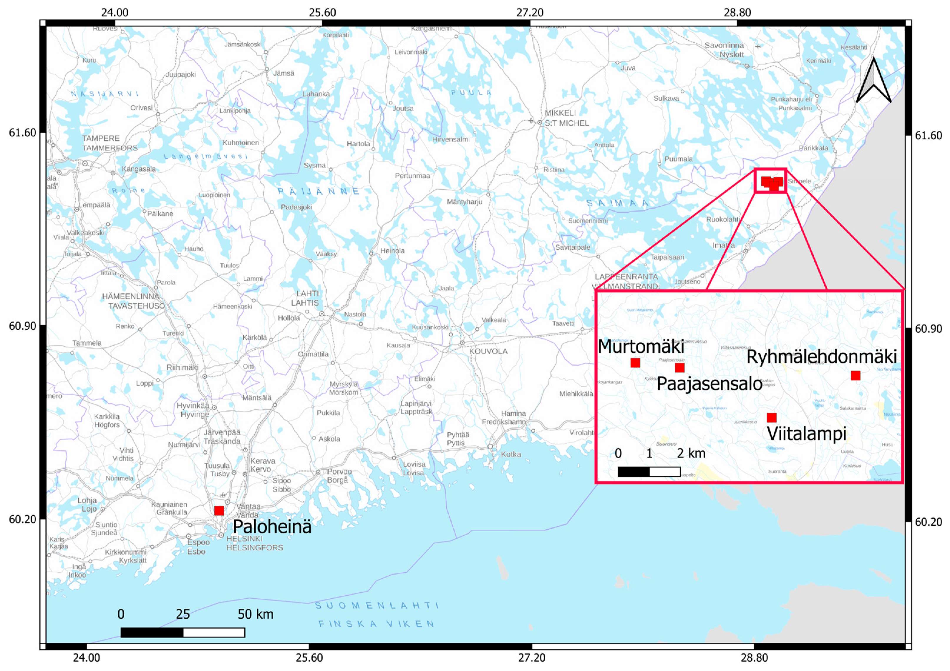
The performance of the YOLO algorithm was evaluated and compared with the results obtained in a previous study [15], where a setting very similar to that used in this study was employed to detect and classify spruce trees into healthy, infested, and dead categories. The F1-scores were 0.788, 0.578, and 0.827 for healthy, infested, and dead trees, respectively, using the data from the Paloheinä, Ruokolahti, and Lahti areas, and the same class-labeling scheme as in the current study. The current study’s F1-scores of 0.706, 0.580, and 0.815 were comparable to these results, with the F1-scores for healthy trees being lower, infested trees being almost the same, and dead trees being slightly lower. The slightly better performance of the YOLO algorithm in [14] can be attributed to the larger dataset used, which also included samples from an additional study area in southern Finland (city of Lahti), as well as for the use of different training and test sets. In the current study, the city of Lahti’s data were not used due to the absence of MS and HS data from the same cameras, whereas considering the training and test sets, they were optimized so that the same trees could be used for the datasets from all sensors. It is worth noting that the previous study [15] reported higher F1-scores of 0.90, 0.79, and 0.98, albeit with a different labeling scheme and solely using Paloheinä data in the test set. The study acknowledges that the results obtained from the Paloheinä data may be somewhat optimistic compared to the data from the other areas. This was attributed to the specific processing techniques applied to the Paloheinä data, which enhanced the detectability of trees in this particular dataset, as well as being due to the better distribution of different health classes.

4.3. Further Research

The development of the proposed method involved several design choices that could affect the outcomes. Data preprocessing was an integral part of the process and included the cropping and resampling of images. These operations could impact the learning capabilities of the models under evaluation. Resampling images to very high or low spatial sizes results in either reduced resolutions or limited convolutional layer sizes. The original tree crown images were of varying sizes, which made the choice of optimal image size challenging. In the end, a compromise was reached by selecting the optimal size for the majority of the images. A further optimization of preprocessing should be considered in future developments.

We did not perform a statistical analysis to determine whether the observed differences in the F1-scores were statistically significant or fell within the margin of experimental errors. To properly establish the significance of the observed variations in the results, hypothesis testing should be conducted in future studies. In addition, the splitting of data into training, validation, and test sets was found to have an impact on the results. This holds true, especially when the amount of data was limited. To ensure that the data split was optimal, efforts were made to ensure that each set had enough samples of each class and that the training and test sets were independent. Ideally, the results should have been cross-validated with several different data splits and multiple rounds of training and testing; however, this was not feasible due to the limited amount of data. Therefore, the reproducibility of the results was not fully addressed in this study. However, it was emphasized that all the results were validated using independent test data.

The limited nature of the data could also impact the comparability of the models that were tested on various image types. The number of samples in each dataset varied, with the RGB dataset having the largest number of samples in each class. The MS dataset contained a slightly lower number of samples of infested trees and a higher number of healthy tree samples than the HS dataset. This disparity could be the primary reason for why the MS 2D-CNN model exhibited a lower F1-score for infested trees and a higher F1-score for healthy trees, compared to the HS 2D-3D-CNN model. To overcome the challenges caused by the insufficient data, future research should focus on collecting a more extensive reference dataset, enabling a more accurate detection of infested classes.

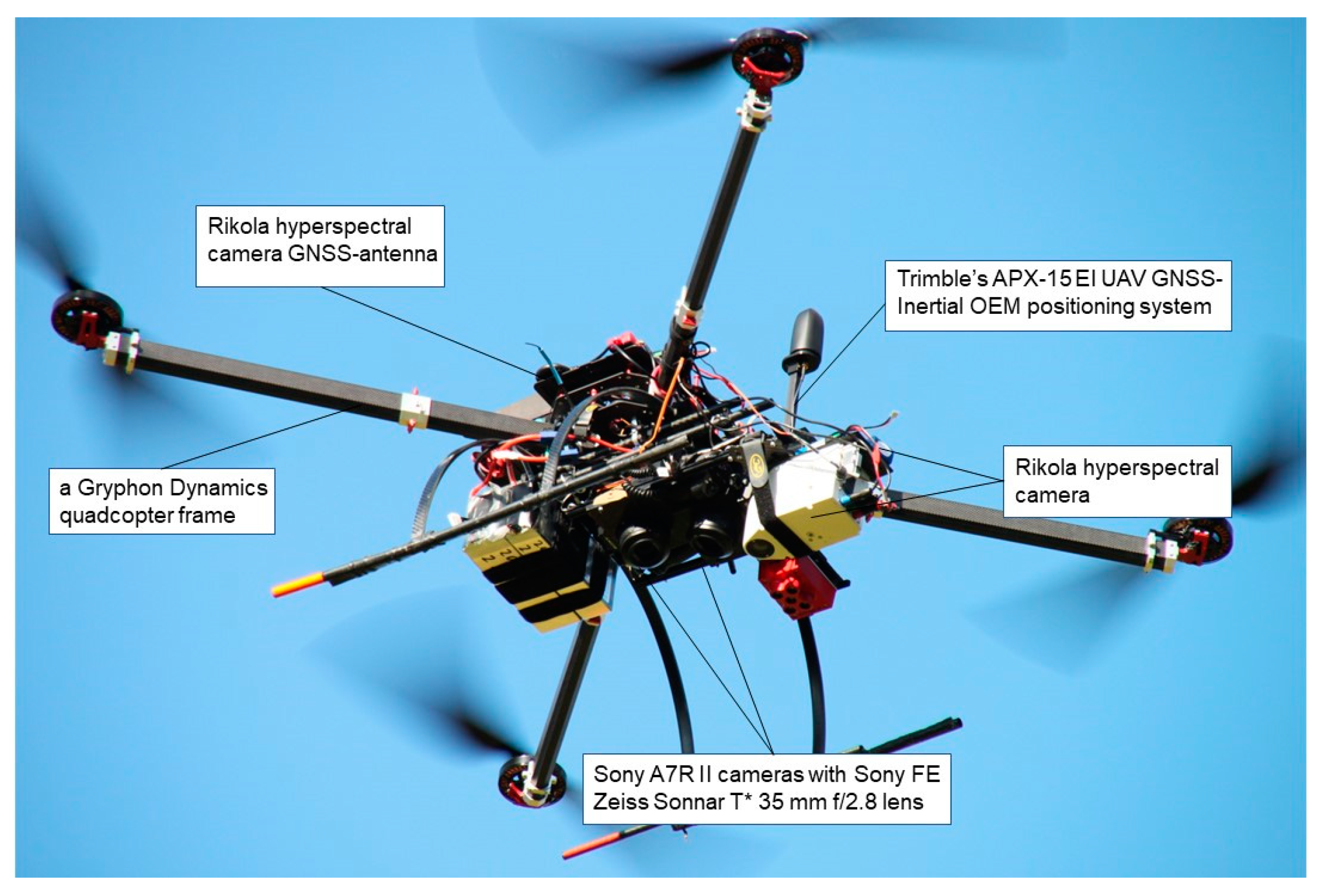
The characteristics of applied camera technology can impact the results of an empirical study. The RGB and MS cameras used in this study represent widely applied camera technologies in UAV remote sensing, thus the obtained results can be considered representative. The HS camera sampled spectral signatures with a relatively high spectral resolution (average of 8.98 nm) and FWHM (average of 6.9 nm) in the visible to near-infrared spectral range (500–900 nm). It is worth recognizing that the state-of-the-art technology offers enhanced-performance figures, for example, a spectral resolution of 2.6 nm and an FWHM of 5.5 nm in the spectral range of 400–1000 nm, as well as extending the spectral range beyond visible and near-infrared to the short-wave-infrared region [59]. Furthermore, this study does not apply spectral-band selection or handcrafted spectral features or indices that are commonly used in the context of classical machine learning approaches [13,20,59]. Instead, we considered that the DNN models could find the relevant features from the spectral signatures. Further studies should evaluate if enhancing camera and spectral qualities, as well as band selection, would be beneficial for assessing tree health.

4.4. Contributions and Outlook

The literature on the classification of bark beetle-infested trees is limited, and to the best of our knowledge, there is no systematic study comparing the performances of RGB, MS, and HS images in this type of tree health assessment task. Furthermore, prior to this study, the use of different network structures for each specific data type had not been investigated in this field. The important contribution of this study is the comprehensive evaluation of several types of deep learning architectures and various remote sensing camera types. The presented results thus provide new information and offer a basis for the further exploration of the use of MS and HS images in detecting bark beetle disturbances using deep learning techniques, as well as for other image classification tasks in the field of remote sensing.

The fundamental need of this research is the development of methods for managing bark beetle outbreaks. For example, in Finland, the outbreaks typically appear in scattered individual trees [15], and therefore high-resolution datasets are required. The UAS-based techniques provided an effective tool to rapidly detect new infestations at the individual tree level. Our results show that dead trees can be reliably detected, even using RGB images. The analysis of multitemporal RGB or MS datasets can be used to detect, understand, and predict the spread of outbreaks. The effective methods for detecting green attacks are still absent from the scientific literature, and HS images, in particular, is expected to be a potential tool for performing this task [9]. Our research will continue to develop strategies for bark beetle management, particularly in terms of developing efficient machine learning and inference pipelines, increasing the datasets for model training, studying the performance of state-of-the-art visible- to shortwave-infrared HS imaging techniques, using novel beyond-visual lines-of-sight drone techniques that enable larger area surveys, as well as developing strategies for green attack detections. Efficient monitoring tools offer knowledge-based decision support to the authorities, politicians, forest owners, and other stakeholders for performing optimized forest management actions in the cases where bark beetle outbreaks continue to spread. This will enable minimizing the negative social, economic, and environmental impacts of bark beetle disturbances.

5. Conclusions

The important contribution of this study is the comprehensive evaluation of several types of deep learning architectures with UAS-acquired RGB, multispectral (MS), and hyperspectral images (HS) to assess the health of individual spruce trees in a test area suffering from a bark beetle outbreak. The presented results thus provide new information and offer a basis for the further exploration of the use of MS and HS images for detecting bark beetle disturbances using deep learning techniques, as well as for other image classification tasks in the field of remote sensing.

The results show that MS and HS images can achieve superior classification outcomes compared to RGB images and identify the most appropriate network structures for each image type. High-accuracy results were obtained for the classifications of healthy and dead trees with all tested camera types, whereas the infested class was often mixed with the healthy class due to the smaller spectral difference between these two classes. Considering the best-performing models with different cameras, the best results for the infested class were obtained using the 2D-3D-CNN 2 model trained on an augmented set of HS images, the next-best results were obtained with the 2D-CNN model trained on an unaugmented set of MS images, and the VGG16 model for augmented RGB images had the lowest performance. The study demonstrated that data augmentation may be used to balance the training class sizes and slightly improve the classification performance, particularly when complex networks with millions of parameters were employed. Additionally, the outcomes reveal that integrating separate classifier networks with the YOLO object detector achieves improved results compared to the YOLO classifier.

The findings of this study offer a basis for the further development of the use of MS and HS images in detecting bark beetle disturbances using deep learning techniques, as well as for other image classification tasks in the field of remote sensing. With the ongoing developments, these technologies have the potential to play a crucial role in forest management efforts to combat large-scale bark beetle outbreaks by providing timely information on the health status of trees.

References

1. Bauman, D.; Fortunel, C.; Delhaye, G.; Malhi, Y.; Cernusak, L.A.; Bentley, L.P.; Rifai, S.W.; Aguirre-Gutiérrez, J.; Menor, I.O.; Phillips, O.L.; et al. Tropical tree mortality has increased with rising atmospheric water stress. Nature 2022, 608, 528–533. [Google Scholar] [CrossRef]
2. Anderegg, W.R.; Wu, C.; Acil, N.; Carvalhais, N.; Pugh, T.A.; Sadler, J.P.; Seidl, R. A climate risk analysis of Earth’s forests in the 21st century. Science 2022, 377, 1099–1103. [Google Scholar] [CrossRef]
3. Patacca, M.; Lindner, M.; Lucas-Borja, M.E.; Cordonnier, T.; Fidej, G.; Gardiner, B.; Hauf, Y.; Jasinevičius, G.; Labonne, S.; Linkevičius, E.; et al. Significant increase in natural disturbance impacts on European forests since 1950. Glob. Chang. Biol. 2023, 29, 1359–1376. [Google Scholar] [CrossRef]
4. Bentz, B.J.; Jönsson, A.M.; Schroeder, M.; Weed, A.; Wilcke, R.A.I.; Larsson, K. Ips typographus and Dendroctonus ponderosae Models Project Thermal Suitability for Intra- and Inter-Continental Establishment in a Changing Climate. Front. For. Glob. Chang. 2019, 2, 1. [Google Scholar] [CrossRef]
5. Hlásny, T.; König, L.; Krokene, P.; Lindner, M.; Montagné-Huck, C.; Müller, J.; Qin, H.; Raffa, K.F.; Schelhaas, M.J.; Svoboda, M.; et al. Bark Beetle Outbreaks in Europe: State of Knowledge and Ways Forward for Management. Curr. For. Rep. 2021, 7, 138–165. [Google Scholar] [CrossRef]
6. Hlásny, T.; Krokene, P.; Liebhold, A.; Montagné-Huck, C.; Müller, J.; Qin, H.; Raffa, K.; Schelhaas, M.-J.; Seidl, R.; Svoboda, M.; et al. Living with Bark Beetles: Impacts, Outlook and Management Options. From Science to Policy 8; European Forest Institute: Joensuu, Finland, 2019. [Google Scholar] [CrossRef]
7. Rogers, B.M.; Solvik, K.; Hogg, E.H.; Ju, J.; Masek, J.G.; Michaelian, M.; Berner, L.T.; Goetz, S.J. Detecting early warning signals of tree mortality in boreal North America using multiscale satellite data. Glob. Chang. Biol. 2018, 24, 2284–2304. [Google Scholar] [CrossRef]
8. Blomqvist, M.; Kosunen, M.; Starr, M.; Kantola, T.; Holopainen, M.; Lyytikäinen-Saarenmaa, P. Modelling the Predisposition of Norway Spruce to Ips typographus L. Infestation by Means of Environmental Factors in Southern Finland. Eur. J. Forest Res. 2018, 137, 675–691. [Google Scholar] [CrossRef]
9. Barta, V.; Hanus, J.; Dobrovolny, L.; Homolova, L. Comparison of field survey and remote sensing techniques for detection of bark beetle-infested trees. For. Ecol. Manag. 2022, 506, 119984. [Google Scholar] [CrossRef]
10. Senf, C.; Seidl, R.; Hostert, P. Remote sensing of forest insect disturbances: Current state and future directions. Int. J. Appl. Earth Obs. Geoinf. 2018, 60, 49–60. [Google Scholar] [CrossRef] [PubMed]
11. Luo, Y.; Huang, H.; Roques, A. Early Monitoring of Forest Wood-Boring Pests with Remote Sensing. Annu. Rev. Entomol. 2023, 68, 277–298. [Google Scholar] [CrossRef]
12. Biedermann, P.H.W.; Muller, J.; Gregoire, J.-C.; Gruppe, A.; Hagge, J.; Hammerbacher, A.; Hofstetter, R.W.; Kandasamy, D.; Kolarik, M.; Kostovcik, M.; et al. Bark Beetle Population Dynamics in the Anthropocene: Challenges and Solutions. Trends Ecol. Evol. 2019, 34, 914–924. [Google Scholar] [CrossRef]
13. Huo, L.; Lindberg, E.; Bohlin, J.; Persson, H.J. Assessing the detectability of European spruce bark beetle green attack in multispectral drone images with high spatial- and temporal resolutions. Remote Sens. Environ. 2023, 287, 113484. [Google Scholar] [CrossRef]
14. Safonova, A.; Hamad, Y.; Alekhina, A.; Kaplun, D. “Detection of Norway Spruce Trees (Picea abies) Infested by Bark Beetle in UAS Images Using YOLOs Architectures. IEEE Access 2022, 10, 10384–10392. [Google Scholar] [CrossRef]
15. Kanerva, H.; Honkavaara, E.; Näsi, R.; Hakala, T.; Junttila, S.; Karila, K.; Koivumäki, N.; Alves Oliveira, R.; Pelto-Arvo, M.; Pölönen, I.; et al. Estimating Tree Health Decline Caused by Ips typographus L. Remote Sens. 2022, 14, 6257. [Google Scholar] [CrossRef]
16. Kloucek, T.; Komarek, J.; Surovy, P.; Hrach, K.; Janata, P.; Vasicek, B. The Use of UAV Mounted Sensors for Precise Detection of Bark Beetle Infestation. Remote Sens. 2019, 11, 1561. [Google Scholar] [CrossRef]
17. Abdollahnejad, A.; Panagiotidis, D. Tree Species Classification and Health Status Assessment for a Mixed Broadleaf-Conifer Forest with UAS Multispectral Imaging. Remote Sens. 2020, 12, 3722. [Google Scholar] [CrossRef]
18. Duarte, A.; Borralho, N.; Cabral, P.; Caetano, M. Recent Advances in Forest Insect Pests and Diseases Monitoring Using UAV-Based Data: A Systematic Review. Forests 2022, 13, 911. [Google Scholar] [CrossRef]
19. Minarik, R.; Langhammer, J.; Lenzioch, T. Detection of Bark Beetle Disturbance at Tree Level Using UAS Multispectral Imagery and Deep Learning. Remote Sens. 2021, 13, 4768. [Google Scholar] [CrossRef]
20. Junttila, S.; Näsi, R.; Koivumäki, N.; Imagholiloo, M.; Saarinen, N.; Raisio, J.; Holopainen, M.; Hyyppä, H.; Hyyppä, J.; Lyytikäinen-Saarenmaa, P.; et al. Multispectral Imagery Provides Benefits for Mapping Spruce Tree Decline Due to Bark Beetle Infestation When Acquired Late in the Season. Remote Sens. 2022, 14, 909. [Google Scholar] [CrossRef]
21. Näsi, R.; Honkavaara, E.; Blomqvist, M.; Lyytikäinen-Saarenmaa, P.; Hakala, T.; Viljanen, N.; Kantola, T.; Holopainen, M. Remote sensing of bark beetle damage in urban forests at individual tree level using a novel hyperspectral camera from UAV and aircraft. Urban For. Urban Green. 2018, 30, 72–83. [Google Scholar] [CrossRef]
22. Ecke, S.; Dempewolf, J.; Frey, J.; Schwaller, A.; Endres, E.; Klemmt, H.-J.; Tiede, D.; Seifert, T. UAV-Based Forest Health Monitoring: A Systematic Review. Remote Sens. 2022, 14, 3205. [Google Scholar] [CrossRef]
23. Georgieva, M.; Belilov, S.; Dimitrov, S.; Iliev, M.; Trenkin, V.; Mirchev, P.; Georgiev, G. Application of Remote Sensing Data for Assessment of Bark Beetle Attacks in Pine Plantations in Kirkovo Region, the Eastern Rhodopes. Forests 2022, 13, 620. [Google Scholar] [CrossRef]
24. Redmon, J.; Divvala, S.; Girshich, R.; Farhadi, A. You Only Look Once: Unified, Real-Time Object Detection. In Proceedings of the IEEE Conference on Computer Vision and Pattern Recognition (CVPR), Las Vegas, NV, USA, 27–30 June 2016; pp. 779–788. [Google Scholar]
25. Junttila, S.; Holopainen, M.; Vastaranta, M.; Lyytikäinen-Saarenmaa, P.; Kaartinen, H.; Hyyppä, J.; Hyyppä, H. The potential of dual-wavelength terrestrial lidar in early detection of Ips typographus (L.) infestation–Leaf water content as a proxy. Remote Sens. Environ. 2019, 231, 111264. [Google Scholar] [CrossRef]
26. Abdullah, H.; Darvishzadeh, R.; Skidmore, A.K.; Groen, T.A.; Heurich, M. European spruce bark beetle (Ips typographus L.) green attack affects foliar reflectance and biochemical properties. Int. J. Appl. Earth Obs. Geoinf. 2018, 64, 199–209. [Google Scholar] [CrossRef]
27. Filella, I.; Penuelas, J. The red edge position and shape as indicators of plant chlorophyll content, biomass and hydric status. Int. J. Remote Sens. 1994, 15, 1459–1470. [Google Scholar] [CrossRef]
28. Honkavaara, E.; Rosnell, T.; Oliveira, R.; Tommaselli, A. Band registration of tuneable frame format hyperspectral UAV imagers in complex scenes. ISPRS J. Photogramm. Remote Sens. 2017, 134, 96–109. [Google Scholar] [CrossRef]
29. Honkavaara, E.; Khoramshahi, E. Radiometric Correction of Close-Range Spectral Image Blocks Captured Using an Unmanned Aerial Vehicle with a Radiometric Block Adjustment. Remote Sens. 2018, 10, 256. [Google Scholar] [CrossRef]
30. Karila, K.; Alves Oliveira, R.; Ek, J.; Kaivosoja, J.; Koivumäki, N.; Korhonen, P.; Niemeläinen, O.; Nyholm, L.; Näsi, R.; Pölönen, I.; et al. Estimating Grass Sward Quality and Quantity Parameters Using Drone Remote Sensing with Deep Neural Networks. Remote Sens. 2022, 14, 2692. [Google Scholar] [CrossRef]
31. Nezami, S.; Khoramshahi, E.; Nevalainen, O.; Pölönen, I.; Honkavaara, E. Tree Species Classification of Drone Hyperspectral and RGB Imagery with Deep Learning Convolutional. Remote Sens. 2020, 12, 1070. [Google Scholar] [CrossRef]
32. Pi, W.; Du, J.; Bi, Y.; Gao, X.; Zhu, X. 3D-CNN based UAS hyperspectral imagery for grassland degradation indicator ground object classification research. Ecol. Inform. 2021, 62, 101278. [Google Scholar] [CrossRef]
33. Zhang, B.; Zhao, L.; Zhang, X. Three-dimensional convolutional neural network model for tree species classification using airborne hyperspectral images. Remote Sens. Environ. 2020, 247, 111938. [Google Scholar] [CrossRef]
34. Yu, C.; Han, R.; Song, M.; Liu, C.; Chang, C.I. A Simplified 2D-3D CNN Architecture for Hyperspectral Image Classification Based on Spatial–Spectral Fusion. IEEE J. Sel. Top. Appl. Earth Obs. Remote Sens. 2020, 13, 2485–2501. [Google Scholar] [CrossRef]
35. Ge, Z.; Cao, G.; Li, X.; Fu, P. Hyperspectral Image Classification Method Based on 2D–3D CNN and Multibranch Feature Fusion. IEEE J. Sel. Top. Appl. Earth Obs. Remote Sens. 2020, 13, 5776–5788. [Google Scholar] [CrossRef]
36. Morales, G.; Sheppard, J.W.; Scherrer, B.; Shaw, J.A. Reduced-cost hyperspectral convolutional neural networks. Appl. Remote Sens. 2020, 14, 036519. [Google Scholar] [CrossRef]
37. Simonyan, K.; Zisserman, A. Very Deep Convolutional Networks for Large-Scale Image Recognition. In Proceedings of the International Conference on Learning Representations (ICLR), San Diego, CA, USA, 7–9 May 2015. [Google Scholar]
38. Dosovitskiy, A.; Beyer, L.; Kolesnikov, A.; Weissenborn, D.; Zhai, X.; Unterthiner, T.; Dehghani, M.; Minderer, M.; Heigold, G.; Gelly, S.; et al. An image is worth 16 × 16 words: Transformers for image recognition at scale. In Proceedings of the International Conference on Learning Representations (ICLR), Vienna, Austria, 4–7 May 2021. [Google Scholar]
39. Deng, J.; Dong, W.; Socher, R.; Li, L.-J.; Li, K.; Fei-Fei, L. Imagenet: A large-scale hierarchical image database. In Proceedings of the 2009 IEEE Conference on Computer Vision and Pattern Recognition (CVPR), Miami, Florida, 20–25 June 2009; pp. 248–255. [Google Scholar]
40. Akiba, T.; Shotaro, S.; Toshihiko, Y.; Takeru, O.; Masanori, K. Optuna: A Next-generation Hyperparameter Optimization Framework. In Proceedings of the 25th ACM SIGKDD International Conference on Knowledge Discovery & Data Mining (KDD), Anchorage, AK, USA, 4–8 August 2019. [Google Scholar]
41. Ozaki, Y.; Nomura, M. Hyperparameter Optimization Methods: Overview and Characteristics. IEICE Trans. 2020, 103, 615–631. [Google Scholar] [CrossRef]
42. Li, L.; Jamieson, K.; Rostamizadeh, A.; Gonina, E.; Ben-Tzur, J.; Hardt, M.; Rechta, B.; Talwalkar, A. A System for Massively Paraller Hyperparameter Tuning. In Proceedings of the Machine Learning and Systems (MLSys), Austin, TX, USA, 2–4 March 2020. [Google Scholar]
43. TorchVision: PyTorch’s Computer Vision Library. Github Repository. 2016. Available online: https://github.com/pytorch/vision (accessed on 29 September 2023).
44. PyTorch Torchvision. Torchvision.Transforms.RandomRotation, Version 0.13.1. Software Package. Available online: https://pytorch.org/vision/stable/transforms.html#randomrotation (accessed on 29 September 2023).
45. PyTorch Torchvision. Torchvision.Transforms.RandomHorizontalFlip, Version 0.13.1. Software Package. Available online: https://pytorch.org/vision/stable/transforms.html#randomhorizontalflip (accessed on 29 September 2023).
46. PyTorch Torchvision. Torchvision.Transforms.RandomVerticalFlip, Version 0.13.1. Software Package. Available online: https://pytorch.org/vision/stable/transforms.html#randomverticalflip (accessed on 29 September 2023).
47. PyTorch Torchvision. Torchvision.Transforms.GaussianBlur, Version 0.13.1. Software Package. Available online: https://pytorch.org/vision/stable/transforms.html#gaussianblur (accessed on 29 September 2023).
48. PyTorch Torchvision. Torchvision.Transforms.Pad, Version 0.13.1. Software Package. Available online: https://pytorch.org/vision/stable/transforms.html#pad (accessed on 29 September 2023).
49. PyTorch Torchvision. Torchvision.Transforms.RandomPerspective, Version 0.13.1. Software Package. Available online: https://pytorch.org/vision/stable/transforms.html#randomperspective (accessed on 29 September 2023).
50. Bochkovskiy, A.; Wang, C.Y.; Liao, H.Y.M. YOLOv4: Optimal Speed and Accuracy of Object Detection. arXiv 2020, arXiv:2004.10934. [Google Scholar]
51. Wang, C.Y.; Liao, H.Y.M.; Wu, Y.H.; Chen, P.Y.; Hsieh, J.W.; Yeh, I.H. CSPNet: A new backbone that can enhance learning capability of CNN. In Proceedings of the IEEE/CVF Conference on Computer Vision and Pattern Recognition Workshops (CVPRW), Seattle, WA, USA, 14–19 June 2020; pp. 390–391. [Google Scholar]
52. Lin, T.Y.; Maire, M.; Belongie, S.; Bourdev, L.; Girshick, R.; Hays, J.; Perona, P.; Zitnick, C.L.; Dollár, P. Microsoft COCO: Common Objects in Context. In Proceedings of the European Conference on Computer Vision (ECCV), Cham, Germany, 6–12 September 2014; pp. 740–755. [Google Scholar]
53. Padilla, R.; Passos, W.L.; Dias, T.L.B.; Netto, S.L.; da Silva, E.A.B. A Comparative Analysis of Object Detection Metrics with a Companion Open-Source Toolkit. Electronics 2021, 10, 279. [Google Scholar] [CrossRef]
54. Sun, Y.; Huang, J.; Ao, Z.; Lao, D.; Xin, Q. Deep Learning Approaches for the Mapping of Tree Species Diversity in a Tropical Wetland Using Airborne LiDAR and High-Spatial-Resolution Remote Sensing Images. Forests 2019, 10, 1047. [Google Scholar] [CrossRef]
55. Alem, A.; Kumar, S. Transfer Learning Models for Land Cover and Land Use Classification in Remote Sensing Image. Appl. Artif. Intell. 2022, 36, 2014192. [Google Scholar] [CrossRef]
56. Reedha, R.; Dericquebourg, E.; Canals, R.; Hafiane, A. Transformer Neural Network for Weed and Crop Classification of High Resolution UAS Images. Remote Sens. 2022, 14, 592. [Google Scholar] [CrossRef]
57. Bazi, Y.; Bashmal, L.; Al Rahhal, M.M.; Al Dayil, R.; Al Ajlan, N. Vision Transformers for Remote Sensing Image Classification. Remote Sens. 2021, 13, 516. [Google Scholar] [CrossRef]
58. Chadwick, A.J.; Coops, N.C.; Bater, C.W.; Martens, L.A.; White, B. Species Classification of Automatically Delineated Regenerating Conifer Crowns Using RGB and Near-Infrared UAS Imagery. IEEE Geosci. Remote. Sens. 2022, 19, 1–5. [Google Scholar] [CrossRef]
59. Oliveira, R.A.; Näsi, R.; Korhonen, P.; Mustonen, A.; Niemeläinen, O.; Koivumäki, N.; Hakala, T.; Suomalainen, J.; Kaivosoja, J.; Honkavaara, E. High-precision estimation of grass quality and quantity using UAS-based VNIR and SWIR hyperspectral cameras and machine learning. Precis. Agric. 2023. [Google Scholar] [CrossRef]
Figure 1. Proposed supervised deep learning workflow for spruce health estimation.
Remotesensing 15 04928 g001
Figure 2. Distribution of the study areas in Helsinki and Ruokolahti. Background map (raster) https://www.maanmittauslaitos.fi/en/opendata-licence-cc40 (accessed on 29 September 2023).
Remotesensing 15 04928 g002
Figure 3. The multisensory UAS with a dual-RGB camera, Rikola hyperspectral camera, and MicaSense RedEdge.
Remotesensing 15 04928 g003
Figure 4. (a) Area cropped from original orthophoto. Reference trees are surrounded by blue bounding boxes. (b) Input image for YOLO network. Unlabeled trees (white areas) are manually removed from the image. Reference trees are depicted with different colors based on class. Green denotes healthy trees, orange infested, and red dead trees.
Remotesensing 15 04928 g004
Figure 5. Tree crown images captured by RGB, MS, and HS cameras with 5, 5, and 10 cm ground sample distances, respectively. MS images have visible color bands (B: 475, G: 560, R: 668 nm) and HS images have false color bands (B: 557.59; G: 648.67; R: 855.44 nm).
Remotesensing 15 04928 g005