Abstract
Grassland aboveground biomass (AGB) is an important indicator for studying the change in grassland ecological quality and carbon cycle. The rapid development of high-resolution remote sensing and unmanned aerial vehicles (UAV) provides a new opportunity for accurate estimation of grassland AGB on the plot scale. In this study, the mountain grassland was taken as the research object. Using UAV Light Detection and Ranging (LiDAR) data and multispectral satellite images, the influence of topographic correction methods on AGB estimation was compared and a series of LiDAR metrics and vegetation indices were extracted. On this basis, a comprehensive indicator, the vegetation index-height-intensity model (VHI), was proposed to estimate AGB quickly. The results show that: (1) Among the four topographic correction methods, the Teillet regression has the best effect, and can effectively improve the accuracy of AGB estimation in mountain grassland. The correlation between corrected ratio vegetation index and AGB was the highest (correlation coefficient: 0.682). (2) Among the height and intensity metrics, median height and max intensity yielded the higher accuracy in estimating AGB, with Root Mean Square Error (RMSE) of 322 g/m2 and 333 g/m2, respectively. (3) The VHI integrated spectrum and LiDAR information, and its accuracy for AGB estimation for mountain grassland, was obviously better than other indicators, with an RMSE of 272 g/m2. We also found that the accuracy of VHI in univariate models was comparable to that of complex multivariate models such as stepwise regression, support vector machine, and random forest. This study provides a new approach for estimating grassland AGB with multi-source data. As a simple and effective indicator, VHI has shown strong application potential for grassland AGB estimating in mountainous areas, and can be further applied to grassland carbon cycle research and fine management.
1. Introduction
Grassland is one of the world’s important terrestrial ecosystem, accounting for about one third of the land surface of the Earth [1] and accounting for about 40% of Chinese total land area [2]. Grassland has an extremely important ecological protection function as a windbreak and for sand fixation, soil and water conservation, carbon fixation and oxygen release, and is also an important source of production materials for people in pastoral areas [3,4]. The research on grassland aboveground biomass (AGB) has long been the focus of attention. The grassland AGB directly reflects the fluctuation of grassland ecological quality and is an important data source for research on the grassland carbon cycle and vegetation net primary productivity [5,6], and can also provide a reliable basis for the policy formulation of grassland management departments. Mountain grassland is one of the important grassland types, and has the characteristics of large biomass, complex topographic conditions, and difficulty in AGB estimation [7,8]. It is also widely distributed in the mountainous areas of southern and western China. The rapid and accurate estimation of AGB in mountain grassland is a challenging research subject, which is of great significance to the estimation of carbon storage and the sustainable development of mountain grassland.
Remote sensing technology has become the main method of grassland AGB estimation because of its advantages of continuous observation capabilities, wide coverage, and low cost. Commonly used remote sensing data sources include MODIS [9], Landsat [10], and other low and medium resolution satellite data. In recent years, with the continuous improvement of sub-meter high-resolution data techniques and the emergence of various unmanned aerial vehicle (UAV) platforms, the efficient and accurate estimation of grassland AGB on the plot scale has become a new research focus [11,12]. This can provide reliable support for fine management of key grassland areas and can also be used as the database for high-precision retrieval of large-scale grassland AGB. However, the current estimation of grassland AGB is mainly based on passive optical remote sensing data and retrieved by establishing the relationship between the field measured AGB and the vegetation index (VI) or a certain band. The traditional multispectral data can reflect the vegetation information on the plane. However, the real vegetation is three-dimensional, and the vegetation information of the vertical structure has widely been proved to be more important in AGB retrieval [13,14].
As a new active remote sensing data source, Light Detection and Ranging (LiDAR) data have been successfully applied to the retrieval of several important vegetation parameters in recent years [15,16]. The LiDAR sensor emits laser pulses to the ground and receives the reflected signals. Based on the sensor height and scanning angle, the three-dimensional position information of the ground objects was calculated. Compared with the traditional photogrammetric techniques, the position information of LiDAR point clouds is more accurate [17]. In the research on AGB, UAV LiDAR has been widely used recently, which can help us obtain the information on the vertical structure of the vegetation and establish the AGB estimation model more accurately. For example, Luo et al. [14] found that the bias of estimating forest AGB was 31.361 Mg/ha using spectral information, while the bias decreased to 15.245 Mg/ha when spectral information was combined with UAV LiDAR data. In addition, UAV LiDAR data also contain the intensity information of ground objects, which was mostly used for landcover classification and species identification [18,19]. In recent years, LiDAR intensity has been used in AGB modeling and has achieved good results. García et al. [20] found that the AGB model of forest combining height and intensity variables provided the lowest errors and highest index of agreement. In general, UAV LiDAR has been widely applied in forests [21], wetland [22], etc., but has rarely appeared in the study of grassland AGB [23,24,25]. On the one hand, the top-to-bottom view of UAV far away from the canopy and the density of grassland vegetation make it difficult for the laser pulse to fully penetrate the canopy. On the other hand, it is hard to detect low-stature vegetation because of the limited time of flight between successive returns. These factors may cause information loss of vegetation and constrain the accuracy of grassland AGB estimation. Another gap is that most of the existing studies were concentrated on AGB estimation of flat terrain, while mountainous areas were rarely involved, especially for mountain grassland.
Due to the influence of mountainous terrain on atmospheric radiation, shadow effect, and multiple scattering, the retrieval of vegetation parameters in mountainous areas faces the problem of reflectance deviation caused by topographic fluctuation [26]. Some studies have simulated the change of pixel reflectivity under different slopes, and the results showed that the maximum relative deviation can reach about 85% [27]. The topographic correction methods can solve the impact of rugged terrain on remote sensing images to varying degrees, which correct the reflectance of pixel to a reference plane (usually horizontal plane) based on the mountain radiation transmission model or the solar radiation geometric transformation. Since the digital elevation model (DEM) was first introduced into the Minnaert model in 1980, by using the slope cosine relationship [28], there have been many topographic correction methods, which can be divided into empirical models, semi-empirical models, and physical models. In comparison, physical models have received more attention in recent years, because researchers pay more attention to the transferability and mathematical simplification of models. For example, Li et al. [29], Couturier et al. [30] and Yin et al. [31] have put forward the latest physical models, respectively, in recent years, and can effectively correct topographic effects in different regions. However, most of the previous studies focused on the comparison of topographic correction algorithms of medium-resolution remote sensing data, and rarely analyzed them in sub-meter images. In the high-resolution data sources, the topographic effect will be more dramatic due to the influence of texture, shadow, and spectral variation [32], and the effect of topographic correction methods may be different from that of medium-resolution images. In addition, the influence of the topographic effect on the grassland AGB retrieval has rarely been studied and discussed.
To sum up, the main research gaps in grassland AGB estimation are the lack of vegetation vertical structure to improve accuracy, and the insufficient research on the impact of rugged terrain on AGB estimation. In this paper, a typical area of mountain grassland in southern China was selected as the study area. The overall goal is to propose a method for estimating AGB of herbaceous vegetation in rugged terrain using the combination of LiDAR data and multispectral data. Additionally, three objectives are established to accomplish this goal: (1) to test the effect of topographic correction models on the estimation of mountain grassland AGB, and identify the optimal correction model and VI in the study area; (2) to extract various LiDAR metrics, evaluate their accuracy in AGB estimation and identify the optimal height metric and intensity metric; and (3) to construct a comprehensive indicator to estimate AGB and evaluate its performance in different regression models.
2. Materials and Methods
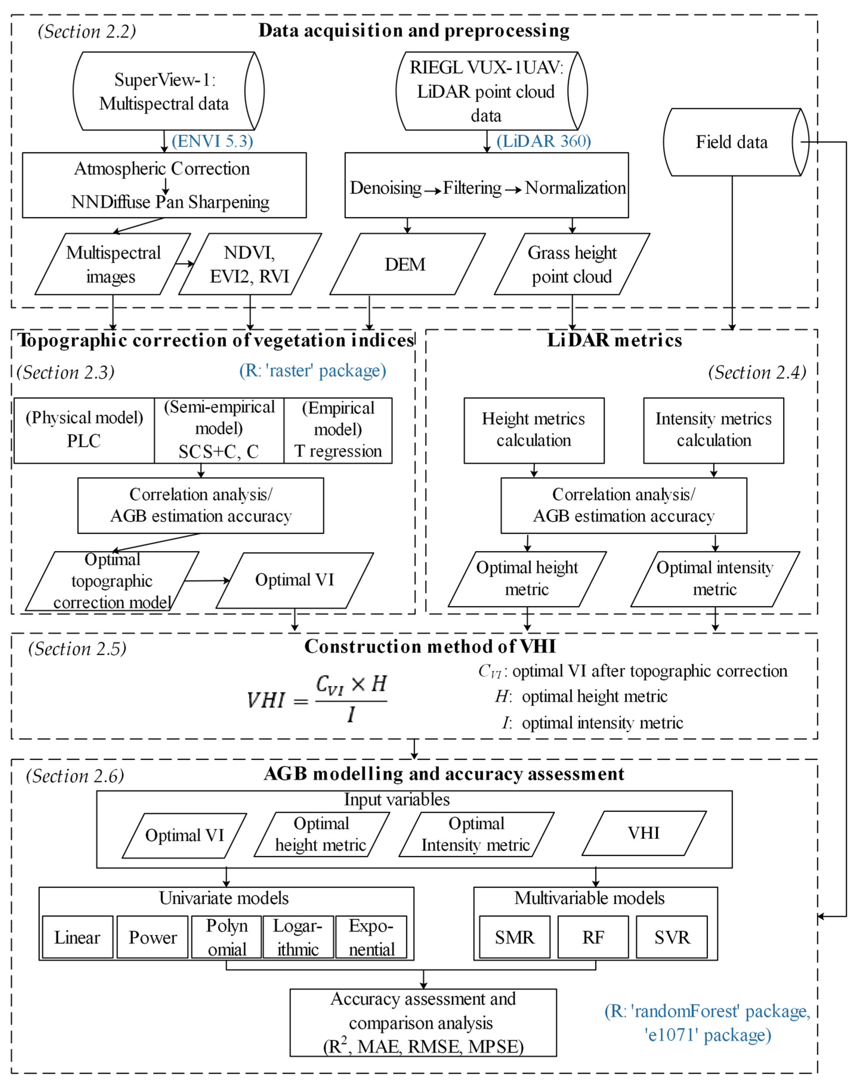
The flowchart of this study is shown in Figure 1. It presents five steps for estimating AGB of mountain grassland based on UAV LiDAR and multispectral images, i.e., (1) data acquisition and preprocessing; (2) topographic correction of vegetation indices; (3) LiDAR metrics; (4) construction method of VHI; (5) AGB modelling and accuracy assessment.
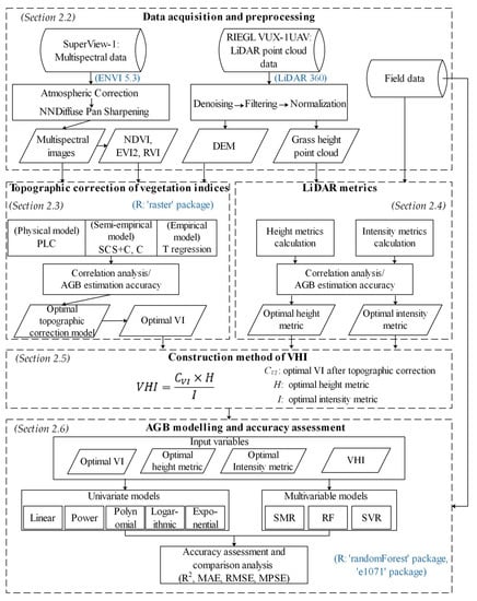
Figure 1.
Flowchart of data processing and AGB estimation (The title of each step is highlighted in boldface. The main software used in the processing are highlighted in blue).
2.1. Study Area
The study area is located in Xingan County, Guilin City, Guangxi Province, in the south of China (Figure 2), with a total grassland area of about 20 km2. The annual total precipitation is about 1800 mm, and the average temperature is about 19 °C, making it a subtropical monsoon climate with abundant water and heat. The study area is located at the top of the mountain and the terrain fluctuates greatly, with the average altitude about 1100 m. The grassland type is tropical tussock grassland, and the main vegetation includes Stipa bungeana Trin., Imperata koenigii (Retz.) Beauv., etc. The average height of the grass is between 20 cm and 80 cm, and the vegetation coverage and AGB are both high. It is a representative area of the mountain grassland in the south of China. In addition, wind power equipment was built on mountain ridges in the area, with a height of 100 m and an interval of 200 m to 500 m. The research on the AGB retrieval method in this area is helpful for accurately grasping the dynamic changes of the vast mountain grassland in China at the plot scale, and also provides a reference for AGB retrieval based on multi-source data under complex topographic conditions.
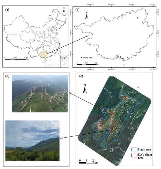
Figure 2.
Location of the study area. (a). location of Guangxi in China; (b). location of the study area in Guangxi; (c). SuperView-1 image of the study area; (d). digital photos of the study area.
2.2. Data Acquisition and Preprocessing
2.2.1. Field Data
Field sampling was conducted after the UAV flight in late July 2021. A total of 89 quadrats were uniformly arranged within the flight area of UAV, each 1 m × 1 m. The measured parameters of each quadrat included longitude and latitude of the central point, altitude, minimum height of the grass, mean height of the grass, maximum height of the grass, vegetation coverage, and AGB. The fractional vegetation coverage (FVC) was measured by five experts using visual estimation, and the average value was taken as the final result. The AGB was clipped at the ground level and then determined by using a high-precision balance. The coordinates were measured by using handheld positioning and navigation system (Qmini A5, Guangzhou Hi-Target Satellite Navigation Technology Co., Ltd., Guangzhou, China), and the positioning accuracy was within 1 m. In order to analyze the influence of topography on VIs and AGB retrieval, the quadrats were selected with different slopes from 0° to 33°. The descriptive statistics of field measured parameters are shown in Table 1.

Table 1.
Descriptive statistics of field measured parameters.
2.2.2. LiDAR Data
Before the field sampling, the DJI Matrice 600 integrates a RIEGL VUX-1UAV sensor, adopted to collect LiDAR data. The sensor adopts a pulse range principle using a near-infrared laser beam and integrates with an AP15(X) inertial navigation system. The field angle of view is 330°, the ranging accuracy is 25 mm, and the maximum ranging is 1050 m. The flight height of UAV is about 200 m, the flight speed is 8 m/s, the width of scanning strip is 214 m, the side overlap is 20%, the average point cloud density is 78 points/m2 of all echoes. Five flights were conducted in the study area, with the total scanning area of 2.5 km2.
The processing of LiDAR point clouds was mainly completed using LiDAR360 (GreenValley International Inc.). Firstly, the original point clouds of each UAV flight were merged. The easily-identified abnormal point cloud was manually clipped. For other abnormal points, the denoising tool, based on statistical outlier removal, was used to denoise the original point clouds. Secondly, the progressive triangulation algorithm was used to filter the denoised point clouds, and the point clouds was classified to ground points and vegetation points. Thirdly, the point clouds were normalized according to the ground points; that is, the elevation of each vegetation point subtracted the elevation of the nearest ground point. The normalized point clouds were later used to extract the vertical structure information of the grass. Finally, the digital elevation model (DEM) was generated by interpolation of ground points using the irregular triangulation algorithm, and the spatial resolution was 0.25 m. The results show that the R2 between DEM and field measured altitude reached 0.9996. DEM was used for topographic correction of multispectral images.
2.2.3. Multispectral Data
SuperView-1 was selected to provide multispectral data, which is a commercial satellite of the China Aerospace Science and Technology Corporation. The image of SuperView-1 has a width of 12 km, 0.5 m spatial resolution in panchromatic band, and 2 m spatial resolution in multispectral bands, including four bands of blue, green, red and near-infrared. Two SuperView-1 images used in this study were acquired on 6 June 2021, with cloud cover of 0%. The solar zenith and azimuth angles were 13.1° and 99.3°. Although the image acquisition time is about 40 days earlier than the field sampling, they are all in the vigorous growth period of the grassland in the study area and the spectral difference can still reflect the AGB change of different quadrats, which will not affect the AGB retrieval.
The preprocessing of SuperView-1 images was completed in ENVI5.3, and ortho correction, radiometric calibration, atmospheric correction, image fusion, and geometric correction were carried out successively. The FLAASH model was used for atmospheric correction, NNDiffuse Pan Sharpening was used for the fusion of multispectral and panchromatic images, and the point cloud data were used as the reference data to carry out geometric correction. Finally, a multispectral image with 0.5 m spatial resolution of the study area was obtained. Normalized Difference Vegetation Index (NDVI), Ratio Vegetation Index (RVI), and Enhanced Vegetation Index 2 (EVI2) were calculated for AGB retrieval. The calculation formulas are as follows:
where denotes the reflectance of red band, and denotes the reflectance of near-infrared band.
2.3. Topographic Correction of Vegetation Indices
One of the most significant advantages of UAV LiDAR data is that they can provide high-precision and high-resolution topographic data. Based on the DEM in Section 2.2.2, four representative topographic correction methods were conducted in this study, using multispectral images, and four groups of corrected NDVI, RVI and EVI2 data were calculated, respectively. Path length correction (PLC) is a new physical model proposed by Yin et al. [33], which is based on the classical radiation transfer theory and assumes that the vegetation canopy is composed of uniformly distributed leaves, and further simplifies the radiation transfer equation into a BRDF (Bidirectional Reflectance Distribution Function) correction formula. Teillet regression is an empirical statistical correction method, which is based on the relationship between the image reflectance and the cosine value of the solar incidence angle, and which converts the reflectance of the slope pixel to the horizontal plane [30]. Two semi-empirical models were selected in this study, which have certain physical significance, but some parameters need to be estimated by empirical methods. The C model proposed by Teillet et al. [34] uses the empirical parameter C to reduce the over correction phenomenon in the shadow area based on the Cosine model. Soenen et al. [35] also introduced parameter C for improvement on the basis of the Sun-Canopy-Sensor (SCS) [36] model. The calculation formulas of the four topographic correction methods are in Table 2. All methods were implemented in R environment by ‘raster’ package.

Table 2.
Expressions of topographic correction methods.
In Table 2, is the reflectance of the original image, is the reflectance of the corrected image, is the average of the original image reflectance, is the solar zenith, is the slope, and is the cosine of solar incidence angle, calculated as follows:
where is the solar azimuth angle, and is the aspect. and can be regressed as follows:
The parameter C is the ratio of b and a. A total of 2500 points were randomly selected to fit Equation (5). In the PLC model, and are the path lengths along solar and viewing directions over flat terrain, and and are their counterparts over sloping terrain. As for flat terrain, the path length can be calculated as a function of the solar zenith angle:
As for sloping terrain, the path length can be calculated as follows:
2.4. LiDAR Metrics
When extracting LiDAR metrics, we adopted a point-based method rather than canopy height model (CHM) to avoid the variation of height being smoothed. After experiments and combining the results of previous related studies [22], the height threshold was set to 0 m in this study; that is, the normalized LiDAR points above 0 m were selected to extract the vegetation height and intensity metrics. Additionally, the optimal radius plot was 1.8 m by comparing different thresholds. The vertical structure of vegetation is an important input variable in the AGB retrieval model. A total of 12 grass height metrics (Table 3) were selected for further analysis, including the minimum height of grass (Hmin), the mean height of grass (Hmean), the maximum height of grass (Hmax), the standard deviation of grass height (Hsd), the variation coefficient of grass height (Hcv), and the percentile of grass height (Hp).

Table 3.
Metrics derived from the LiDAR data used for estimating biomass.
The intensity of the point clouds is the amount of energy returned by ground objects to the LiDAR system. In this study, the intensity information of the point cloud data were taken as one of the important input variables of the AGB retrieval model. It is necessary to correct the intensity data before using them, especially in the mountainous area with complex terrain, as the uncorrected intensity data will cause a significant error in the estimation of vegetation parameters. In order to eliminate the influence of the flight path and angle of incidence, the intensity data were corrected using the following formula:
where is the corrected intensity value, is the original intensity value, is the distance from sensor to object, is the average flying altitude of UAV, and is the incident angle. For the corrected intensity data, the same metrics as grass height were selected for analysis (Table 3).
2.5. Construction Method of VHI
In previous AGB studies, metrics of vegetation structure and vegetation indices were usually inputted into the retrieval model as separate variables [20,22], some researchers only used the structure information of vegetation obtained from point clouds to construct the retrieval model [37], and there are also studies that combine vegetation spectral information with structure information to synthesize an AGB retrieval indicator and achieved good results [17]. However, the above studies were all carried out in limited sample areas, and focused on the woodland or farmland with flat and regular plots, and lack of exploration for rapid acquisition of large-scale and complex topographic conditions of herbaceous vegetation AGB.
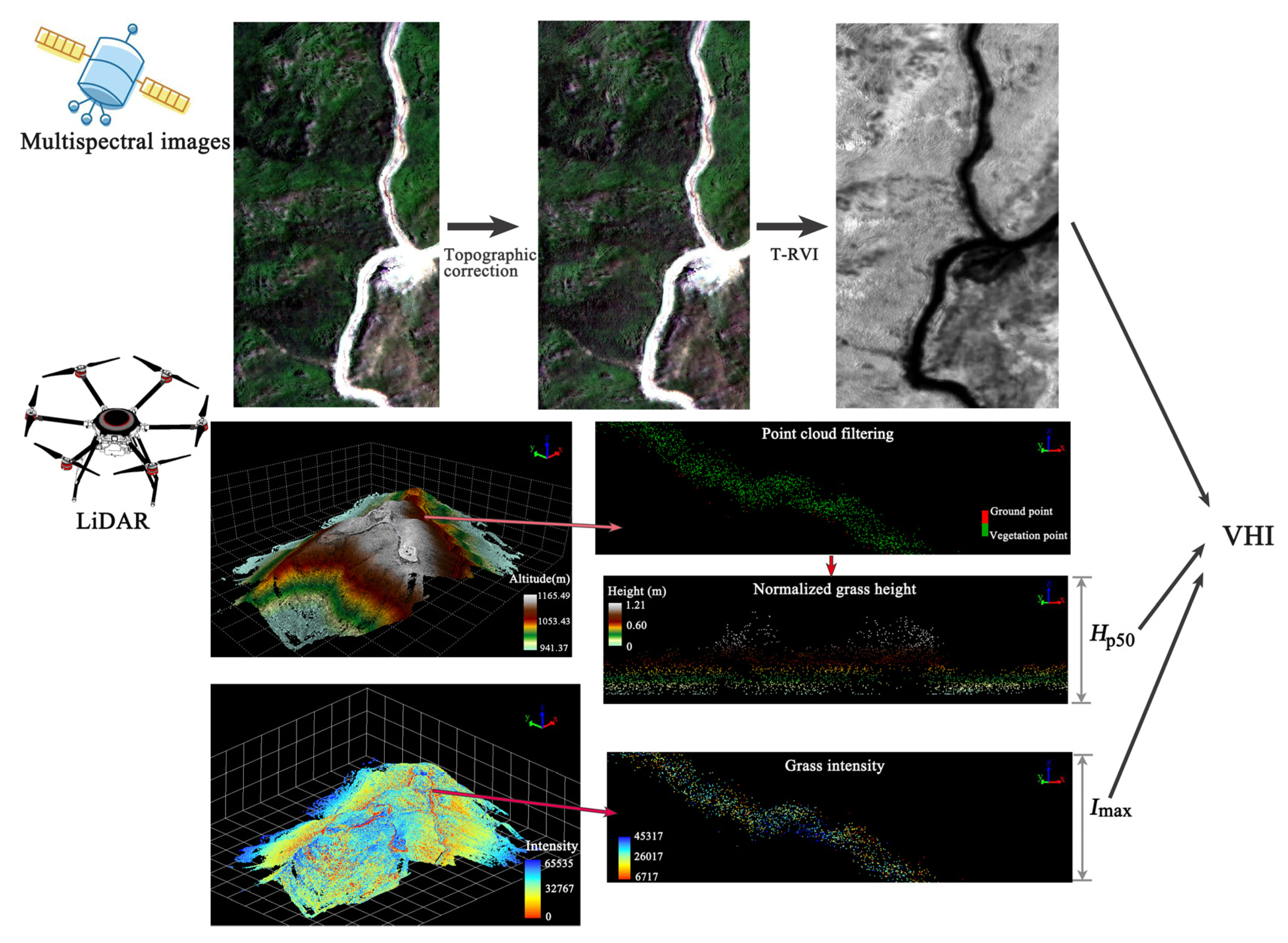
Based on LiDAR and multispectral data, this study attempted to propose a VI-height-intensity model (VHI) as a comprehensive indicator to quickly and accurately retrieve grassland AGB under complex topographic conditions (Figure 3). The VHI is calculated as follows:
where is the mean value of optimal VI after topographic correction, is the optimal height metric, is the optimal intensity metric. Unlike most studies [24,38,39] that directly selected VI and Hmean to retrieve AGB and ignored the importance of point clouds intensity, VHI is simple and takes full advantages of LiDAR and multispectral data. During the VHI calculation, the optimal LiDAR metrics in the study area were selected according to the comparison results, and the topographic correction methods were also compared to select the best VI.
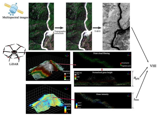
Figure 3.
The workflow plot of the proposed VHI for biomass estimation.
2.6. Methods of AGB Modelling and Accuracy Assessment
In this study, five commonly used univariate models were used to estimate AGB for each VI and for LiDAR metrics, including linear, power, polynomial, logarithmic, and exponential models. In addition, Spearman’s rank-order correlation analysis was used to investigate the relationship between these variables and AGB. The VHI was constructed using the metrics with high model accuracy and strong correlation. Three complex multivariable models, stepwise linear regression (SMR), random forest (RF), and support vector regression (SVR), were also selected in this study for comparative analysis. RF and SVR have been widely used in AGB estimation [40,41], and have their own advantages in dealing with regression problems. RF does not tend to over fit, and can produce the ranking of variable importance. SVR is robust to outliers, and the model has excellent generalization ability. Additionally, SMR has been proved to outperform other machine learning algorithms in estimating grassland AGB using LiDAR data [42]. In the research, we chose these three algorithms to train multivariable complex models and compare them with univariate models based on VHI. All models were built in R environment. In the RF model, ntree was set as 500 and mtry was set as the number of variables divided by 3. In the SVR model, the kernel function was linear, and gamma was 1 divided by the number of variables.
Due to the limited number of samples, the leave-one-out cross-validation (LOOCV) was selected for model training and accuracy validation. LOOCV was conducted 89 modeling times, one sample was selected for validation and the rest of the samples for training in each trial. This method can accurately evaluate the prediction ability of the model. Coefficient of determination (R2), mean absolute error (MAE), root mean square error (RMSE) and mean percent standard error (MPSE) were selected for accuracy verification. These four verification methods were widely used in AGB research [43,44], and their definitions and characteristics are shown in Table 4.

Table 4.
Measures used for accuracy verification.
3. Results
3.1. Comparison of Vegetation Indices for AGB Estimation before and after Topographic Correction
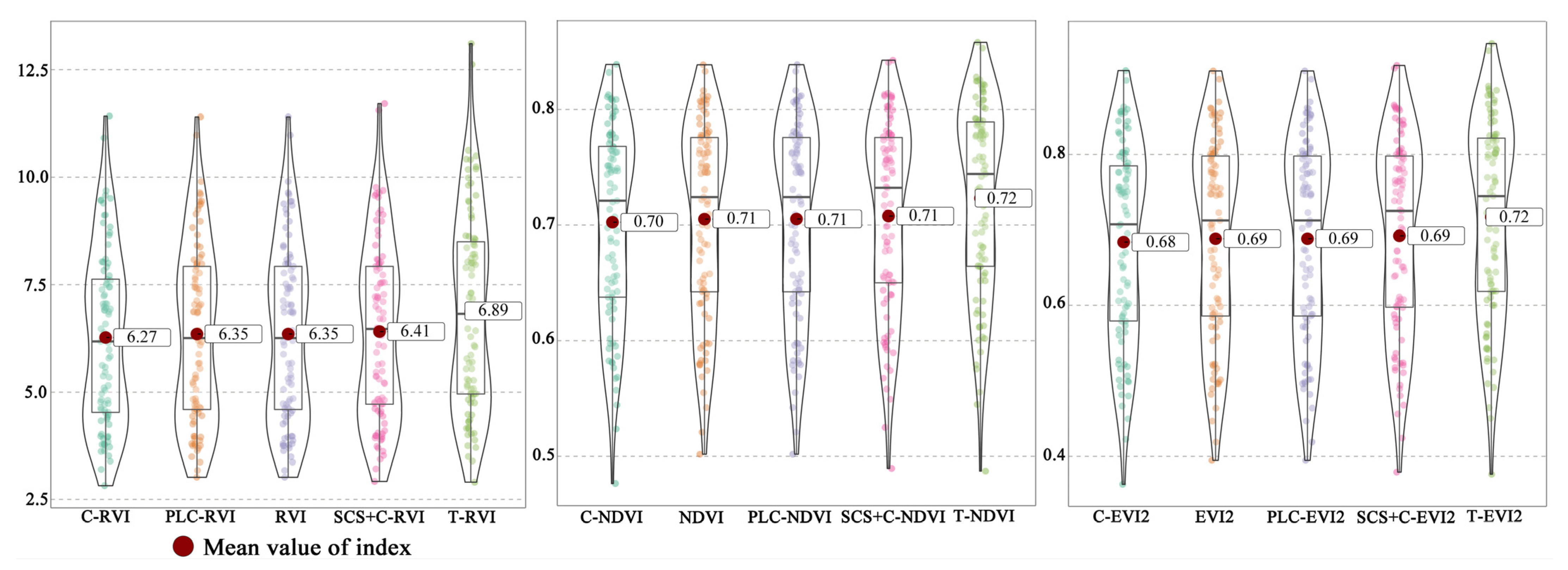
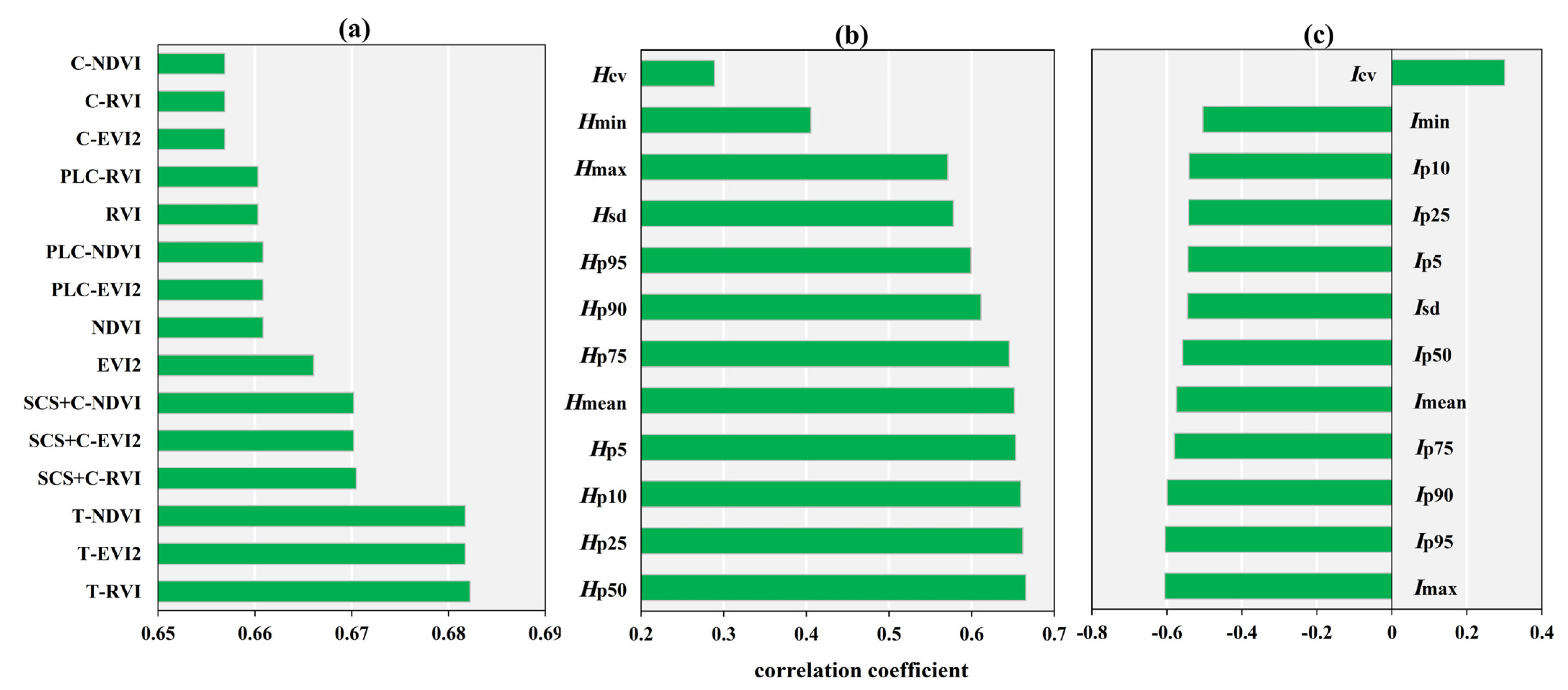
The distribution of VI values before and after topographic correction of the 89 quadrats is shown in Figure 4. The mean value of original RVI is 6.35, the mean value of original NDVI is 0.71, and the mean value of original EVI2 is 0.69. Among the four topographic correction methods, the mean VI value after C correction was lower than the original value, which was similar to the original VI value after PLC and SCS + C correction. The mean VI value after Teillet regression was bigger, especially for the quadrats with large original VI values. Figure 5a shows the ranking of correlation coefficients of VIs before and after topographic correction. Teillet regression was obviously the most effective method. The correlation coefficient between the corrected T-RVI, T-EVI2, T-NDVI and AGB reached 0.682, which was higher than the original EVI2 (0.666), NDVI (0.661), and RVI (0.660). The correlation coefficient of SCS + C corrected VI also improved, and reached 0.670. However, the correlation coefficient of VI and AGB after PLC and C correction decreased.
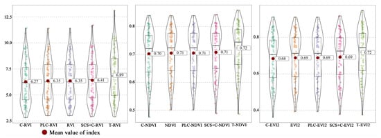
Figure 4.
Vegetation index value of quadrats before and after topographic correction (arranged from left to right according to the mean value of vegetation index).

Figure 5.
Correlation coefficient between metrics and AGB (a). vegetation indices; (b). height metrics; (c). intensity metrics.
Table S1 in the Supplementary File shows the accuracy of five simple univariate AGB retrieval models of VIs before and after topographic correction. The lowest RMSE results can be obtained for the VIs corrected by Teillet regression (around 315 g/m2). The VIs after SCS + C correction also performed well, with MAE and RMSE reduced. However, the accuracy of C-VI and PLC-VI was basically the same as that of original VIs. The above results showed that Teillet regression and SCS + C are more suitable for topographic correction in the study area, while the PLC and C models are not effective.
3.2. Height and Intensity Data for AGB Estimation
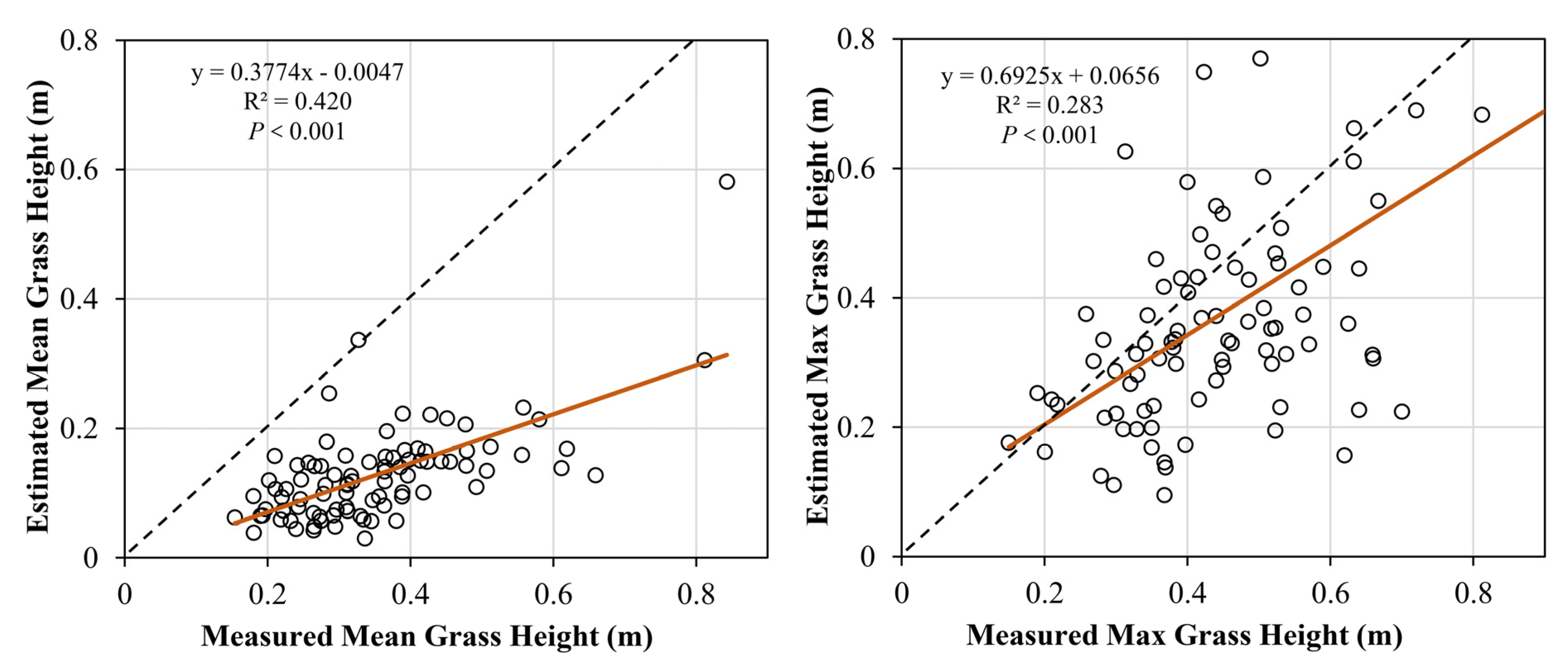
Figure 6 shows the relationship between the LiDAR estimated and field measured grass height. The mean grass height obtained by LiDAR was systematically underestimated and was concentrated below 0.2 m, but it still has a strong linear relationship with the measured value, which can reflect the change trend of grass height of the quadrats. This is similar to the results when using LiDAR point clouds to extract the height of low-stature vegetation in some studies [13,25]. The underestimation of the maximum grass height obtained by LiDAR in this study was reduced, but the fitting result between the LiDAR estimated and field measured value was poor.
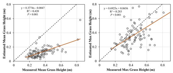
Figure 6.
Relationship between LiDAR-derived and field-measured grass height (brown lines are linear fit curves).
Figure 5b,c, respectively, show the ranking of correlation coefficients between height and intensity metrics and AGB. The correlation coefficients between height metrics and AGB were mostly higher than 0.6, of which Hp50 was the highest, reaching 0.666. Intensity metrics were negatively correlated with AGB, and the correlation was relatively weak. Most of the correlation coefficients of the intensity metrics were between −0.4 and −0.6, of which Imax has the strongest correlation, reaching −0.606. In addition, the results in Figure 5 show that the average level of grass height had a stronger correlation with AGB, while Hmax, Hmin did not reflect AGB well in the vertical structure. The correlation between the high value of intensity and AGB was stronger, and the correlation coefficient basically decreased from Imax downward.
Tables S2 and S3 in the Supplementary File, respectively, show the accuracy verification results of height and intensity metrics in five simple univariate AGB retrieval models. For height metrics, the RMSE of Hp50 in the logarithmic model was the lowest (322 g/m2), while the RMSE of each exponential model was higher than that of the other. For intensity metrics, there was no significant difference in the accuracy performance of different models. Imax, Ip95, Ip90 yielded higher accuracy, with RMSE around 335 g/m2.
3.3. VHI for AGB Estimation
According to the analysis results in Section 3.1 and Section 3.2, T-RVI, Hp50, and Imax were used to construct VHI. Before AGB modelling, normal distribution test and multiple collinearity test were carried out using SPSS 21.0. The results showed that T-RVI, Hp50, and Imax were all normally distributed and had no multicollinearity. Table 5 shows the accuracy verification results of T-RVI, Hp50, Imax, and VHI for estimating AGB in five simple univariate models, and compares the performance in three multivariate models: SMR, SVR, and RF. The expression of each model was randomly selected using LOOCV, and the average values of R2, MAE, RMSE, MPSE over 89 trials were calculated.

Table 5.
Validation statistics of regression models for AGB estimation (The model with the lowest RMSE for each type of input variable is highlighted in boldface).
In all the optimal univariate models, the metrics and AGB showed a nonlinear relationship. The prediction bias of VHI in all univariate models was significantly lower than that of T-RVI (RMSE of the same model decreases by 52 g/m2 at most), Hp50 (RMSE of the same model decreases by 99 g/m2 at most), and Imax (RMSE of the same model decreases by 66 g/m2 at most). VHI in the polynomial model obtained the highest R2 (0.517), and the lowest prediction bias (RMSE = 273 g/m2). In the three multivariable models, T-RVI + Hp50 + Imax and T-RVI + Hp50 + Imax + VHI were all tested. The results showed that the prediction bias of the three models were reduced to a certain extent after adding the VHI (RMSE decreased 7–10 g/m2). SMR obtained the lowest RMSE (281 g/m2) among the three models. However, the improvement of model complexity did not improve the prediction accuracy, and the accuracy of all multivariable models was not better than that of VHI in simple univariate models.
Figure 7a shows the scatter plot of the predicted and the measured AGB of the optimal models from different input variables, and Figure 7b is the corresponding ridgeline plot. The scatter plots show that the four variables were prone to overestimate in the low AGB values and underestimate in the high AGB values. The results of Hp50 and Imax were the most significant, and the prediction results of VHI alleviated this problem. From the ridgeline plot, it can be seen that the AGB prediction values of Hp50 and Imax were concentrated in the range of 600–800 g/m2, and the T-RVI prediction values had two distribution peaks at about 600 and 900 g/m2. The distribution of the predicted values of VHI was the closest to those measured in the field, but the underestimation was still significant for the quadrats above 1500 g/m2.
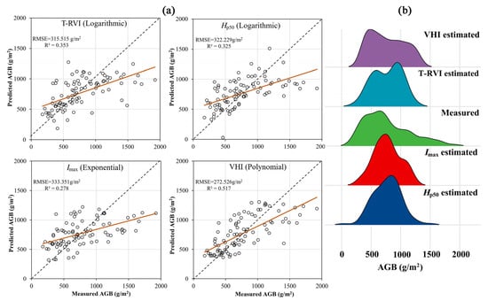
Figure 7.
The scatter plots for measured versus predicted AGB (a) (brown lines are linear fit curves), and ridgeline plot for the distribution of AGB (b).
All the above results show the advantages of VHI as a single indicator that is easy to calculate in the estimation of AGB in mountain grassland. Compared with a single VI or LiDAR metric, it can be more effectively used for rapid modeling and retrieval.
4. Discussion
4.1. Effect of Topographic Correction for AGB Estimation in Fine Scale
Based on the high-precision DEM acquired by UAV LiDAR, this study compared the effects of four representative topographic correction methods on improving the accuracy of AGB estimation. Empirical models are generally considered to have insufficient theoretical basis and lack clear physical meaning, and different models need to be established under different conditions [45]. For example, in the Teillet regression refers to the theoretical reflectivity of flat terrain. Since it is difficult to obtain in mountainous areas, the average reflectance is taken to represent . However, the results of this paper showed that the traditional empirical model (Teillet regression) has the best effect on improving the accuracy of AGB estimation, while the recently proposed physical model (PLC) had no effect. In addition, random points were used to calculate the correlation between the vegetation indices and the cosine of the solar incidence angle (Table 6), and the larger correlation coefficient indicated a bigger topographic effect. Only the correlation coefficients after the correction of the PLC model increased, while the correlation coefficients decreased the most after the correction of the Teillet regression. It indicated that Teillet regression effectively reduced the topographic effect of VIs, but the PLC model had barely any no effect. Moreover, the VIs corrected by the semi-empirical models (C and SCS + C) also significantly reduced the impact of terrain. The result shows that, although the empirical model is difficult to popularize in a large area, it may produce better results at a fine scale based on very high-resolution images. Despite the physical model based on the radiation transmission theory with clear physical significance yielding good performance in multiple regional scale studies [33,46], it may be difficult to effectively eliminate the topographic effect on the fine scale.

Table 6.
Correlation coefficient (r) between vegetation indices and the cosine of the local solar incidence angle before and after topographic correction (low correlation coefficient indicates small topographic effect).
The effect of topographic correction is also affected by some other factors. Previous studies have shown that vegetation indices with no band ratio form are more susceptible to topographic fluctuations [32,47]. This phenomenon was not observed in this study, and there was no significant difference in the performance of the three vegetation indices in the AGB model. The landcover also has a great impact on the topographic correction models. Some studies have found that the landcover stratification can improve the correction effect of Teillet regression, which might be the reason for the better performance of Teillet regression in this study. In addition, most of the current correction models are built on the Lambertian assumption, while the land surface in the real environment is non-Lambertian. The BRDF information can be introduced to improve the effect of correction. In general, the performance of each model in the previous studies varied with different data sources and environments. Although the empirical model showed the best correction result and improved the accuracy of the AGB estimation in this study, it still needs to use more simulated images to explore the optimal method of topographic correction using very high-resolution data and the impact on the retrieval of important ecological indicators.
4.2. Advantages of VHI for AGB Estimation
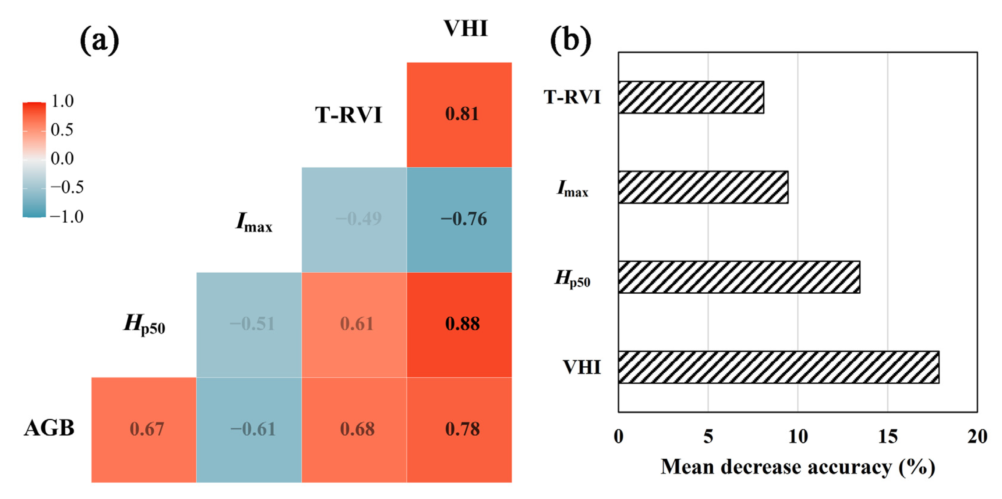
The mutual correlation analysis results are shown in Figure 8a. Compared with the optimal VI, height metric, and intensity metric, the correlation between VHI and AGB reached more than 0.78, significantly higher than the three sub-indicators. The correlation coefficient among the three sub-indicators was relatively low, with the highest correlation coefficient of 0.61 between T-RVI and Hp50, while the average correlation coefficient between VHI and the three sub-indicators reached 0.82. Figure 8b shows the importance ranking of VHI and the optimal VI, height metric, and intensity metric in the RF model. VHI was the most important variable in the RF model. When VHI was randomly disturbed, the out-of-bag error was the largest, which reached 18.95%. The importance of Hp50 and Imax was lower, and T-RVI was the least important in the RF model. The above results show that VHI can comprehensively represent the three sub-indicators and has higher importance in the AGB retrieval model.
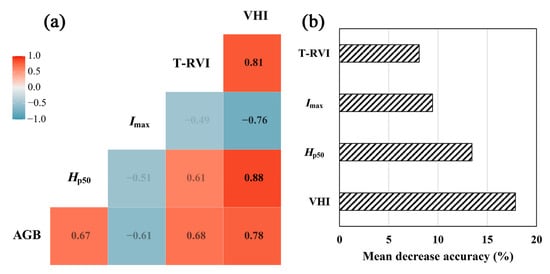
Figure 8.
Correlation plot (a), and the importance of variables in RF model (b).
We also selected two indicators commonly used in previous studies to compare with VHI. Some studies [24] found that the optimal retrieval indicator of AGB can be obtained by multiplying the mean value of VI and height. The calculation formula is as follows:
where is the original VI with the strongest correlation with AGB (EVI2). In addition, researchers [17] found that the volume indicator (CVMVI) constructed by the pixel accumulation of canopy height and VI can retrieve AGB with higher accuracy. In this study, the CHM was obtained in LiDAR360, using the method of normalization based on DEM. The pixels above 0 m within the quadrat buffer area were selected, and the CVMVI was calculated as follows:
where is the EVI2 value of pixel i, is the area of pixel , and is the height of pixel .
Table 7 shows the best accuracy result of VH and CVMVI in five univariate models. The optimal models of the two indicators were obtained by logarithmic regression. The lowest RMSE of VH was 300 g/m2, and the lowest RMSE of CVMVI was 307 g/m2. Compared with the results in Table 5, the accuracy of the above two indicators is better than that of the single VI or LiDAR metric, but lower than that of VHI. It shows that the estimation of grassland AGB by VHI proposed in this paper under rugged terrain performed better than VH and CVMVI.

Table 7.
Validation results for AGB estimation using different variables.
4.3. Analysis of Possible Factors Affecting AGB Estimation
Unlike the previous grassland research based on LiDAR data, which is characterized by flat terrain, small range, and low biomass, AGB retrieval of mountain grassland is a new challenge. Although the VHI proposed in this study effectively improved the accuracy of AGB estimation of mountain grassland, it was still limited by some factors.
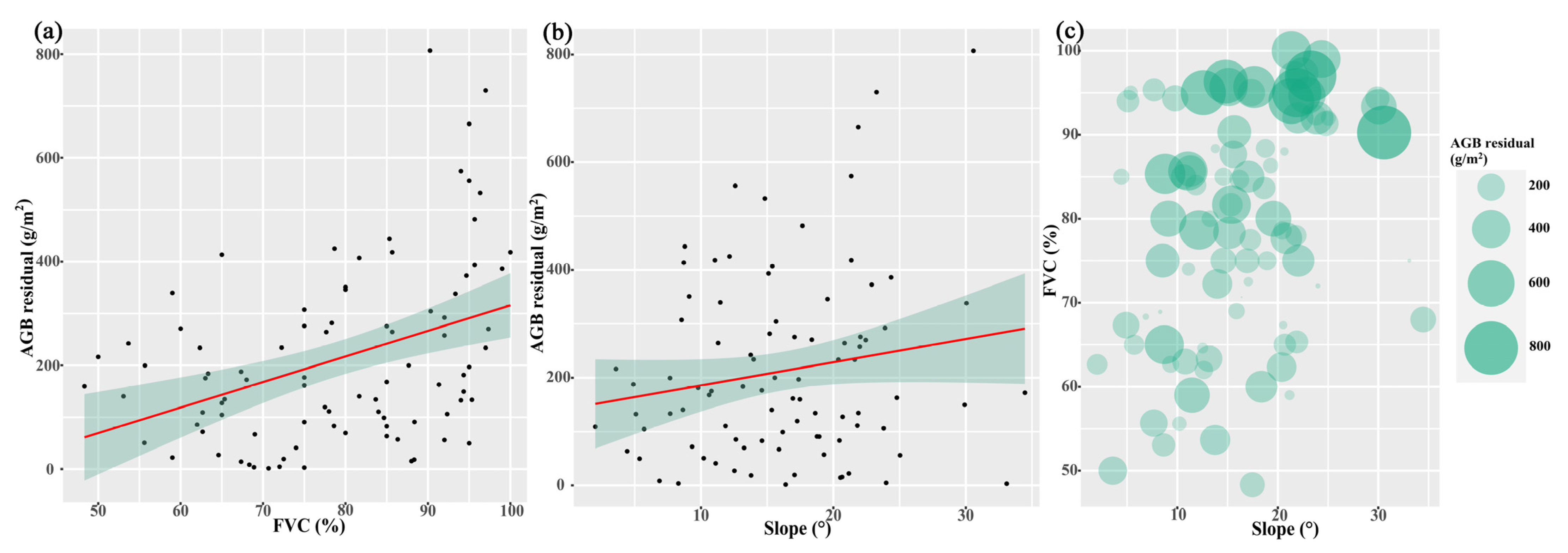
FVC is an important factor affecting the accuracy of AGB estimation. The scatter plot in Figure 9a shows that the residual of AGB estimated by the optimal VHI model displays an increasing trend with the increase of FVC of the quadrats. Especially for the quadrats with FVC greater than 90%, the AGB residual reached more than 500 g/m2. It may be caused by the saturation phenomenon of VI in a densely vegetated area. In addition, the dense and uniform vegetation leads to a difficulty in the laser pulse penetrating the grass to the ground [48,49]. The reduction of ground LiDAR points caused the large estimation bias of canopy height in the high vegetation coverage area. Slope is another important factor in this study. The scatter plot of Figure 9b shows that the residual of AGB increases with the increase of the slope. The slope and aspect between pixels and within pixels caused by topography have a direct impact on the estimation of vegetation parameters, especially in high spatial resolution images. Additionally, the point clouds density could be affected by the relative height difference brought by undulating terrain [25]. The Bubble plot in Figure 9c shows the distribution of AGB residuals under different FVC and slope conditions. It can be found that the quadrats with large residuals are concentrated in the top right corner of the plot, i.e., the area with high FVC and a large slope, which also illustrates the difficulty of accurate retrieval of AGB in mountain grassland.
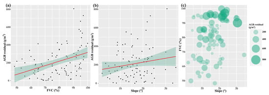
Figure 9.
Scatter plot of AGB residual and FVC (a), scatter plot of AGB residual and slope (b), and bubble plot of AGB residual, FVC, and slope (c).
In addition to the above two factors, there are other factors that restrict the further improvement of accuracy in this study. For example, there is wind-power equipment in the study area, so it is difficult to reduce the flight height and increase the point cloud density to ensure the flight safety of the UAV. More complex retrieval models such as deep learning algorithms combined with VHI may perform better.
5. Conclusions
This study took mountain grassland as the research object, and a fast and accurate AGB estimation method was proposed by using UAV LiDAR and high-resolution multispectral data. The main conclusions are as follows:
(1) Based on the high-precision DEM obtained from LiDAR data, four methods were used to correct the impact of topography on grassland AGB estimation in high-resolution images. The results showed that the effect of empirical models was better than that of semi-empirical and physical models. Compared with the original VI, the RMSE of AGB estimation reduced about 10 g/m2 using the VI corrected by the Teillet regression.
(2) Height and intensity metrics were evaluated by their correlation coefficients with AGB and performance in AGB retrieval models. The average level of grass height and the high value of intensity had a stronger correlation with AGB. For height metrics, the RMSE of Hp50 in the logarithmic model was the lowest (322 g/m2). For intensity metrics, Imax yielded higher accuracy, with RMSE around 333 g/m2.
(3) Based on the optimal VI after topographic correction, and the optimal height and intensity metrics, a synthesized indicator, VHI, was proposed to estimate the AGB of mountain grassland. Compared with the original VI, LiDAR metrics, and the other indicators proposed in previous studies, VHI can effectively improve the estimation accuracy of AGB in mountain grassland. The construction method of VHI is simple and integrates the optimal spectral and LiDAR information. The accuracy of the VHI in univariate models was not lower than that of the complex multivariate models (RF, SVM, SMR).
The method developed in this study showed high application potential in grassland AGB estimation, especially in mountain grassland. The comparison results of topographic correction methods can provide reference for future AGB estimation in rugged terrain based on high-resolution images. Although the VHI proposed in this study yielded high accuracy, it needs to be tested in various mountain grasslands. Additionally, the optimal AGB estimation model was based on empirical models, which may not be directly used in different environments.
The AGB estimation of mountain grassland is still faced with constraints such as high FVC and rugged terrain. A terrain-following mode of UAV LiDAR is an option for future study to overcome the topography impact. In addition, full-waveform LiDAR data can be used to further improve overall accuracy, since they contain more information.
Supplementary Materials
The following supporting information can be downloaded at: https://www.mdpi.com/article/10.3390/rs15020405/s1, Table S1: Validation statistics of vegetation indices; Table S2: Validation statistics of height metrics; Table S3: Validation statistics of intensity metrics.
Author Contributions
Conceptualization, A.C. and X.Y.; methodology, A.C. and X.W.; software, A.C. and X.W.; formal analysis, A.C.; investigation, A.C., X.W., M.Z., J.G., X.X., D.Y., H.Z., Z.H. and Z.J.; resources, X.Y.; writing—original draft preparation, A.C.; writing—review and editing, A.C.; funding acquisition, X.Y. All authors have read and agreed to the published version of the manuscript.
Funding
This work was supported by the Third Xinjiang Scientific Expedition Program (2022xjkk0402) and the National Natural Science Foundation of China (No. 41571105, 41861019).
Data Availability Statement
The data presented in this study are available on request from the corresponding author.
Conflicts of Interest
The authors declare no conflict of interest.
References
- Reinermann, S.; Asam, S.; Kuenzer, C. Remote Sensing of Grassland Production and Management-A Review. Remote Sens. 2020, 12, 1949. [Google Scholar] [CrossRef]
- Jin, Y.X.; Yang, X.C.; Qiu, J.J.; Li, J.Y.; Gao, T.; Wu, Q.; Zhao, F.; Ma, H.L.; Yu, H.D.; Xu, B. Remote Sensing-Based Biomass Estimation and Its Spatio-Temporal Variations in Temperate Grassland, Northern China. Remote Sens. 2014, 6, 1496–1513. [Google Scholar] [CrossRef]
- Lopez, B.; Hines, P.J.; Ash, C. The unrecognized value of grass. Science 2022, 377, 590–591. [Google Scholar] [CrossRef] [PubMed]
- Ma, W.H.; Fang, J.Y.; Yang, Y.H.; Mohammat, A. Biomass carbon stocks and their changes in northern China’s grasslands during 1982–2006. Sci. China Life Sci. 2010, 53, 841–850. [Google Scholar] [CrossRef]
- Kong, B.; Yu, H.; Du, R.X.; Wang, Q. Quantitative Estimation of Biomass of Alpine Grasslands Using Hyperspectral Remote Sensing. Rangel. Ecol. Manag. 2019, 72, 336–346. [Google Scholar] [CrossRef]
- Xia, J.Z.; Ma, M.N.; Liang, T.G.; Wu, C.Y.; Yang, Y.H.; Zhang, L.; Zhang, Y.J.; Yuan, W.P. Estimates of grassland biomass and turnover time on the Tibetan Plateau. Environ. Res. Lett. 2018, 13, 014020. [Google Scholar] [CrossRef]
- Schirpke, U.; Kohler, M.; Leitinger, G.; Fontana, V.; Tasser, E.; Tappeiner, U. Future impacts of changing land-use and climate on ecosystem services of mountain grassland and their resilience. Ecosyst. Serv. 2017, 26, 79–94. [Google Scholar] [CrossRef]
- Ward, A.; Yin, K.S.; Dargusch, P.; Fulton, E.A.; Aziz, A.A. The Impact of Land Use Change on Carbon Stored in Mountain Grasslands and Shrublands. Ecol. Econ. 2017, 135, 114–124. [Google Scholar] [CrossRef]
- Liang, T.G.; Yang, S.X.; Feng, Q.S.; Liu, B.K.; Zhang, R.P.; Huang, X.D.; Xie, H.J. Multi-factor modeling of above-ground biomass in alpine grassland: A case study in the Three-River Headwaters Region, China. Remote Sens. Environ. 2016, 186, 164–172. [Google Scholar] [CrossRef]
- Quan, X.W.; He, B.B.; Yebra, M.; Yin, C.M.; Liao, Z.M.; Zhang, X.T.; Li, X. A radiative transfer model-based method for the estimation of grassland aboveground biomass. Int. J. Appl. Earth Obs. Geoinf. 2017, 54, 159–168. [Google Scholar] [CrossRef]
- Meyer, H.; Lehnert, L.W.; Wang, Y.; Reudenbach, C.; Nauss, T.; Bendix, J. From local spectral measurements to maps of vegetation cover and biomass on the Qinghai-Tibet-Plateau: Do we need hyperspectral information? Int. J. Appl. Earth Obs. Geoinf. 2017, 55, 21–31. [Google Scholar] [CrossRef]
- Sinde-Gonzalez, I.; Gil-Docampo, M.; Arza-Garcia, M.; Grefa-Sanchez, J.; Yanez-Simba, D.; Perez-Guerrero, P.; Abril-Porras, V. Biomass estimation of pasture plots with multitemporal UAV-based photogrammetric surveys. Int. J. Appl. Earth Obs. Geoinf. 2021, 101, 102355. [Google Scholar] [CrossRef]
- Kulawardhana, R.W.; Popescu, S.C.; Feagin, R.A. Fusion of lidar and multispectral data to quantify salt marsh carbon stocks. Remote Sens. Environ. 2014, 154, 345–357. [Google Scholar] [CrossRef]
- Luo, S.Z.; Wang, C.; Xi, X.H.; Pan, F.F.; Peng, D.L.; Zou, J.; Nie, S.; Qin, H.M. Fusion of airborne LiDAR data and hyperspectral imagery for aboveground and belowground forest biomass estimation. Ecol. Indic. 2017, 73, 378–387. [Google Scholar] [CrossRef]
- Han, W.Q.; Zhao, S.H.; Feng, X.Z.; Chen, L. Extraction of multilayer vegetation coverage using airborne LiDAR discrete points with intensity information in urban areas: A case study in Nanjing City, China. Int. J. Appl. Earth Obs. Geoinf. 2014, 30, 56–64. [Google Scholar] [CrossRef]
- Luo, S.Z.; Chen, J.M.; Wang, C.; Gonsamo, A.; Xi, X.H.; Lin, Y.; Qian, M.J.; Peng, D.L.; Nie, S.; Qin, H.M. Comparative Performances of Airborne LiDAR Height and Intensity Data for Leaf Area Index Estimation. Ieee J. Sel. Top. Appl. Earth Obs. Remote Sens. 2018, 11, 300–310. [Google Scholar] [CrossRef]
- Maimaitijiang, M.; Sagan, V.; Sidike, P.; Maimaitiyiming, M.; Hartling, S.; Peterson, K.T.; Maw, M.J.W.; Shakoor, N.; Mockler, T.; Fritschi, F.B. Vegetation Index Weighted Canopy Volume Model (CVMVI) for soybean biomass estimation from Unmanned Aerial System-based RGB imagery. ISPRS J. Photogramm. Remote Sens. 2019, 151, 27–41. [Google Scholar] [CrossRef]
- Luo, S.Z.; Wang, C.; Xi, X.H.; Zeng, H.C.; Li, D.; Xia, S.B.; Wang, P. Fusion of Airborne Discrete-Return LiDAR and Hyperspectral Data for Land Cover Classification. Remote Sens. 2016, 8, 3. [Google Scholar] [CrossRef]
- Zhao, K.G.; Popescu, S. Lidar-based mapping of leaf area index and its use for validating GLOBCARBON satellite LAI product in a temperate forest of the southern USA. Remote Sens. Environ. 2009, 113, 1628–1645. [Google Scholar] [CrossRef]
- Garcia, M.; Riano, D.; Chuvieco, E.; Danson, F.M. Estimating biomass carbon stocks for a Mediterranean forest in central Spain using LiDAR height and intensity data. Remote Sens. Environ. 2010, 114, 816–830. [Google Scholar] [CrossRef]
- Wulder, M.A.; White, J.C.; Nelson, R.F.; Naesset, E.; Orka, H.O.; Coops, N.C.; Hilker, T.; Bater, C.W.; Gobakken, T. Lidar sampling for large-area forest characterization: A review. Remote Sens. Environ. 2012, 121, 196–209. [Google Scholar] [CrossRef]
- Luo, S.Z.; Wang, C.; Xi, X.H.; Pan, F.F.; Qian, M.J.; Peng, D.L.; Nie, S.; Qin, H.M.; Lin, Y. Retrieving aboveground biomass of wetland Phragmites australis (common reed) using a combination of airborne discrete-return LiDAR and hyperspectral data. Int. J. Appl. Earth Obs. Geoinf. 2017, 58, 107–117. [Google Scholar] [CrossRef]
- Maesano, M.; Khoury, S.; Nakhle, F.; Firrincieli, A.; Gay, A.; Tauro, F.; Harfouche, A. UAV-Based LiDAR for High-Throughput Determination of Plant Height and Above-Ground Biomass of the Bioenergy Grass Arundo donax. Remote Sens. 2020, 12, 464. [Google Scholar] [CrossRef]
- Zhang, X.; Bao, Y.H.; Wang, D.L.; Xin, X.P.; Ding, L.; Xu, D.W.; Hou, L.L.; Shen, J. Using UAV LiDAR to Extract Vegetation Parameters of Inner Mongolian Grassland. Remote Sens. 2021, 13, 656. [Google Scholar] [CrossRef]
- Zhao, X.X.; Su, Y.J.; Hu, T.Y.; Cao, M.Q.; Liu, X.Q.; Yang, Q.L.; Guan, H.C.; Liu, L.L.; Guo, Q.H. Analysis of UAV lidar information loss and its influence on the estimation accuracy of structural and functional traits in a meadow steppe. Ecol. Indic. 2022, 135, 108515. [Google Scholar] [CrossRef]
- Wen, J.G.; Liu, Q.H.; Liu, Q.; Xiao, Q.; Li, X.W. Parametrized BRDF for atmospheric and topographic correction and albedo estimation in Jiangxi rugged terrain, China. Int. J. Remote Sens. 2009, 30, 2875–2896. [Google Scholar] [CrossRef]
- Hao, D.L.; Wen, J.G.; Xiao, Q.; Wu, S.B.; Lin, X.W.; Dou, B.C.; You, D.Q.; Tang, Y. Simulation and Analysis of the Topographic Effects on Snow-Free Albedo over Rugged Terrain. Remote Sens. 2018, 10, 278. [Google Scholar] [CrossRef]
- Smith, J.; Lin, T.; Ranson, K. The lambertian assumption and landsat data. Photogramm. Eng. Remote Sens. 1980, 46, 1183. [Google Scholar]
- Li, A.N.; Wang, Q.F.; Bian, J.H.; Lei, G.B. An Improved Physics-Based Model for Topographic Correction of Landsat TM Images. Remote Sens. 2015, 7, 6296–6319. [Google Scholar] [CrossRef]
- Yin, G.F.; Li, A.N.; Zhao, W.; Jin, H.A.; Bian, J.H.; Wu, S.B.A. Modeling Canopy Reflectance Over Sloping Terrain Based on Path Length Correction. IEEE Trans. Geosci. Remote Sens. 2017, 55, 4597–4609. [Google Scholar] [CrossRef]
- Couturier, S.; Gastellu-Etchegorry, J.P.; Martin, E.; Patino, P. Building a Forward-Mode Three-Dimensional Reflectance Model for Topographic Normalization of High-Resolution (1–5 m) Imagery: Validation Phase in a Forested Environment. IEEE Trans. Geosci. Remote Sens. 2013, 51, 3910–3921. [Google Scholar] [CrossRef]
- Matsushita, B.; Yang, W.; Chen, J.; Onda, Y.; Qiu, G.Y. Sensitivity of the Enhanced Vegetation Index (EVI) and Normalized Difference Vegetation Index (NDVI) to topographic effects: A case study in high-density cypress forest. Sensors 2007, 7, 2636–2651. [Google Scholar] [CrossRef] [PubMed]
- Yin, G.F.; Li, A.N.; Wu, S.B.; Fan, W.L.; Zeng, Y.L.; Yan, K.; Xu, B.D.; Li, J.; Liu, Q.H. PLC: A simple and semi-physical topographic correction method for vegetation canopies based on path length correction. Remote Sens. Environ. 2018, 215, 184–198. [Google Scholar] [CrossRef]
- Teillet, P.M.; Guindon, B.; Goodenough, D.G. On the Slope-Aspect Correction of Multispectral Scanner Data. Can. J. Remote Sens. 1981, 8, 84–106. [Google Scholar] [CrossRef]
- Soenen, S.A.; Peddle, D.R.; Coburn, C.A. SCS+C: A modified sun-canopy-sensor topographic correction in forested terrain. Ieee Trans. Geosci. Remote Sens. 2005, 43, 2148–2159. [Google Scholar] [CrossRef]
- Gu, D.; Gillespie, A. Topographic Normalization of Landsat TM Images of Forest Based on Subpixel Sun–Canopy–Sensor Geometry. Remote Sens. Environ. 1998, 64, 166–175. [Google Scholar] [CrossRef]
- Jimenez-Berni, J.A.; Deery, D.M.; Rozas-Larraondo, P.; Condon, A.G.; Rebetzke, G.J.; James, R.A.; Bovill, W.D.; Furbank, R.T.; Sirault, X.R.R. High Throughput Determination of Plant Height, Ground Cover, and Above-Ground Biomass in Wheat with LiDAR. Front. Plant Sci. 2018, 9, 237. [Google Scholar] [CrossRef]
- Zhu, Y.H.; Zhao, C.J.; Yang, H.; Yang, G.J.; Han, L.; Li, Z.H.; Feng, H.K.; Xu, B.; Wu, J.T.; Lei, L. Estimation of maize above-ground biomass based on stem-leaf separation strategy integrated with LiDAR and optical remote sensing data. PeerJ 2019, 7, e7593. [Google Scholar] [CrossRef]
- Michez, A.; Lejeune, P.; Bauwens, S.; Herinaina, A.A.L.; Blaise, Y.; Munoz, E.C.; Lebeau, F.; Bindelle, J. Mapping and Monitoring of Biomass and Grazing in Pasture with an Unmanned Aerial System. Remote Sens. 2019, 11, 473. [Google Scholar] [CrossRef]
- Nandy, S.; Srinet, R.; Padalia, H. Mapping Forest Height and Aboveground Biomass by Integrating ICESat-2, Sentinel-1 and Sentinel-2 Data Using Random Forest Algorithm in Northwest Himalayan Foothills of India. Geophys. Res. Lett. 2021, 48. [Google Scholar] [CrossRef]
- Zhou, W.; Li, H.R.; Xie, L.J.; Nie, X.M.; Wang, Z.; Du, Z.P.; Yue, T.X. Remote sensing inversion of grassland aboveground biomass based on high accuracy surface modeling. Ecol. Indic. 2021, 121, 107215. [Google Scholar] [CrossRef]
- Xu, K.X.; Su, Y.J.; Liu, J.; Hu, T.Y.; Jin, S.C.; Ma, Q.; Zhai, Q.P.; Wang, R.; Zhang, J.; Li, Y.M.; et al. Estimation of degraded grassland aboveground biomass using machine learning methods from terrestrial laser scanning data. Ecol. Indic. 2020, 108, 105747. [Google Scholar] [CrossRef]
- Zeng, W.S.; Zhang, L.J.; Chen, X.Y.; Cheng, Z.C.; Ma, K.X.; Li, Z.H. Construction of compatible and additive individual-tree biomass models for Pinus tabulaeformis in China. Can. J. For. Res. 2017, 47, 467–475. [Google Scholar] [CrossRef]
- Liu, Y.; Feng, H.K.; Yue, J.B.; Li, Z.H.; Yang, G.J.; Song, X.Y.; Yang, X.D.; Zhao, Y. Remote-sensing estimation of potato above-ground biomass based on spectral and spatial features extracted from high-definition digital camera images. Comput. Electron. Agric. 2022, 198, 107089. [Google Scholar] [CrossRef]
- Blesius, L.; Weirich, F. The use of the Minnaert correction for land-cover classification in mountainous terrain. Int. J. Remote Sens. 2005, 26, 3831–3851. [Google Scholar] [CrossRef]
- Chen, R.; Yin, G.F.; Zhao, W.; Xu, B.D.; Zeng, Y.L.; Liu, G.X.; Verger, A. TCNIRv: Topographically Corrected Near-Infrared Reflectance of Vegetation for Tracking Gross Primary Production Over Mountainous Areas. IEEE Trans. Geosci. Remote Sens. 2022, 60, 4409310. [Google Scholar] [CrossRef]
- Zhu, G.L.; Liu, Y.B.; Ju, W.M.; Chen, J.M. Evaluation of topographic effects on four commonly used vegetation indices. J. Remote Sens. 2013, 17, 211–221. [Google Scholar]
- Wang, C.; Menenti, M.; Stoll, M.P.; Feola, A.; Belluco, E.; Marani, M. Separation of Ground and Low Vegetation Signatures in LiDAR Measurements of Salt-Marsh Environments. IEEE Trans. Geosci. Remote Sens. 2009, 47, 2014–2023. [Google Scholar] [CrossRef]
- Hopkinson, C.; Chasmer, L.E.; Sass, G.; Creed, I.F.; Sitar, M.; Kalbfleisch, W.; Treitz, P. Vegetation class dependent errors in lidar ground elevation and canopy height estimates in a boreal wetland environment. Can. J. Remote Sens. 2005, 31, 191–206. [Google Scholar] [CrossRef]
Disclaimer/Publisher’s Note: The statements, opinions and data contained in all publications are solely those of the individual author(s) and contributor(s) and not of MDPI and/or the editor(s). MDPI and/or the editor(s) disclaim responsibility for any injury to people or property resulting from any ideas, methods, instructions or products referred to in the content. |
© 2023 by the authors. Licensee MDPI, Basel, Switzerland. This article is an open access article distributed under the terms and conditions of the Creative Commons Attribution (CC BY) license (https://creativecommons.org/licenses/by/4.0/).

