Abstract
Urban agglomerations, such as Beijing-Tianjin-Hebei Region, Yangtze River Delta and Pearl River Delta, are the key regions for energy conservation, carbon emission reduction and low-carbon development in China. However, spatiotemporal patterns of CO2 emissions at fine scale in these major urban agglomerations are not well documented. In this study, a back propagation neural network based on genetic algorithm optimization (GABP) coupled with NPP/VIIRS nighttime light datasets was established to estimate the CO2 emissions of China’s three major urban agglomerations at 500 m resolution from 2014 to 2019. The results showed that spatial patterns of CO2 emissions presented three-core distribution in the Beijing-Tianjin-Hebei Region, multiple-core distribution in the Yangtze River Delta, and null-core distribution in the Pearl River Delta. Temporal patterns of CO2 emissions showed upward trends in 28.74–43.99% of the total areas while downward trends were shown in 13.47–15.43% of the total areas in three urban agglomerations. The total amount of CO2 emissions in urban areas was largest among urban circles, followed by first-level urban circles and second-level urban circles. The profiles of CO2 emissions along urbanization gradients featured high peaks and wide ranges in large cities, and low peaks and narrow ranges in small cities. Population density primarily impacted the spatial pattern of CO2 emissions among urban agglomerations, followed by terrain slope. These findings suggested that differences in urban agglomerations should be taken into consideration in formulating emission reduction policies.
1. Introduction
Global cities only account for 2% of the Earth’s area, but produce more than 70% of the world’s anthropogenic CO2 emissions [1,2]. The extent and intensity of global climate change will be strengthened in the next few decades, according to the sixth assessment report of the Intergovernmental Panel on Climate Change (IPCC). CO2 emissions are increasing at an unprecedented rate due to the energy consumption related to human activities [3,4,5,6]. The urbanization rate of China increased to 59.6% in 2018 [7]. Rising energy consumption due to the rapid development of urbanization and industrialization has increased China’s CO2 emissions significantly [8,9]. A study reported that China’s 35 largest cities accounted for 40% of the country’s CO2 emissions [10]. The huge amount and rapid growth rate of CO2 emissions have made China face huge pressure to balance economic growth and sustainable development [11,12]. Therefore, exploring the patterns of carbon emissions in urban agglomerations are crucial for formulating carbon reduction policies.
Satellite nighttime light information at high resolution may provide accurate estimation of spatial and temporal patterns of CO2 emissions [13]. The relationships between statistical energy consumption and nighttime light data can be obtained by a variety of regression models [14,15,16]. However, the conventional regression method is not effective due to the fixed model parameters [17]. Back propagation neural networks allow a high variance model without suffering from overfitting, which can provide more accurate regression models than traditional regression models. Jasiński (2019) used artificial neural networks to model electricity consumption based on nighttime light images [18]. Yang et al. (2020) proposed a structure-based neural network ensemble to analyze the nonlinear relationship between nighttime light data and CO2 emissions [17]. Genetic neural networks integrated with the satellite nighttime light data at high resolution and local statistical CO2 emissions data may improve estimation accuracy of CO2 emissions.
Fine-scale information of national and regional scale CO2 emissions is essential for the design of emissions mitigation policies [19,20,21]. Nighttime light data from satellite information is highly associated with the footprint of human activities, and can provide an effective proxy for estimating energy consumption and CO2 emissions [14,15]. The Defense Meteorological Satellite Program’s Operational Linescan System (DMSP/OLS) data have been commonly used for the estimation of carbon emissions [16]. For example, Doll et al. (2000) first found a strong relationship between DMSP/OLS nighttime light data and CO2 emissions [22]. Wang and Liu (2017) utilized DMSP/OLS data from 1992 to 2013 to analyze regional inequalities and spatial agglomeration of urban CO2 emissions [23]. Shi et al. (2018) combined DMSP/OLS images and statistical energy consumption data to explore spatiotemporal variations of CO2 emissions from urban agglomeration to national scales [13]. Soon afterwards, the Suomi National Polar-Orbiting Partnership (NPP) Visible Infrared Imaging Radiometer Suite (VIIRS) using nighttime light data with high spatial resolution and wide radiometric detection proved to be better than DMSP/OLS data in simulating CO2 emissions [24,25]. Shi et al. (2014) analyzed the correlation between nighttime light, gross domestic product (GDP) and electric power consumption, and found that NPP/VIIRS data were powerful tools to model socioeconomic indicators [26]. Zhao et al. (2018) modelled CO2 emissions in residential sectors at the urban scale and found that the performance of NPP/VIIRS data in simulating residential carbon emissions were better than DMSP/OLS data [25].
Beijing-Tianjin-Hebei, the Yangtze River Delta and the Pearl River Delta are the most populated urban agglomerations with the highest comprehensive strength in China. By 2019, the GDP of the three urban agglomerations accounted for 39.65% of the national GDP, while their population accounted for only 23.79% of the national population. Here, spatiotemporal variations of CO2 emissions among urban agglomerations and the profiles of CO2 emissions along urbanization gradients were explored using NPP/VIIRS nighttime light datasets at 500 m resolution from 2014 to 2019 based on a back propagation neural network with genetic algorithm optimization (GABP). Our aims were to: (1) integrate multi-source data to estimate fine-scale carbon emissions of three urban agglomerations; (2) analyze the spatial and temporal dynamics of carbon emissions among urban agglomerations and the profiles of CO2 emissions along urbanization gradients within cities; and (3) reveal the main influencing factors of carbon emissions.
2. Materials and Methods
2.1. Study Area
Beijing-Tianjin-Hebei, the Yangtze River Delta, and the Pearl River Delta regions are China’s three major economic growth poles. These urban agglomerations, located on the eastern coast of Mainland China, are focus areas for energy conservation and emission reduction (Figure 1). Beijing-Tianjin-Hebei consists of two municipalities, Beijing and Tianjin, as well as 11 cities in Hebei province. The Yangtze River Delta consists of 26 cities (i.e., Shanghai, Hangzhou, Nanjing, etc.). The Pearl River Delta is composed of nine cities in Guangdong province. Furthermore, Beijing-Tianjin-Hebei is dominated by temperate continental monsoon climate [27], while the Pearl River Delta and Yangtze River Delta are dominated by subtropical/tropical monsoon climates [28] and maritime monsoon subtropical climates [29], respectively.
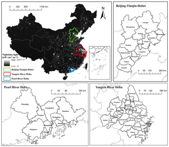
Figure 1.
Locations of three urban agglomerations such as Beijing-Tianjin-Hebei Region, Yangtze River Delta, and Pearl River Delta.
2.2. Data Sources
Datasets consisted of NPP/VIIRS nighttime light data, fossil fuel combustion data, socioeconomic data, and basic geographic information data. Monthly NPP/VIIRS nighttime light data (vcmsl version) at 500 m resolution during 2014–2019 were obtained from Colorado School of Mines (https://payneinstitute.mines.edu/eog, accessed on 11 October 2019). The radiation value of pixels in this data represents the intensity of the light. The fossil fuel combustion data and socioeconomic data were obtained from China Statistical Yearbook, China Regional Statistical Yearbook, and statistical yearbooks of each city. The details of these data are listed in Table 1.

Table 1.
Data used in this study.
2.3. Methods
The flowchart of this study is summarized in Figure 2. Three key steps are included: (1) estimating the statistical carbon emissions using the IPCC method; (2) estimating CO2 emissions using GABP neural networks coupled with satellite data and statistical carbon emissions; (3) exploring the spatiotemporal dynamics of CO2 emissions at 500 m resolution and their influencing factors.
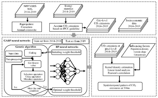
Figure 2.
The flowchart of this study.
2.3.1. Correction of NPP/VIIRS Nighttime Light Data
The NPP/VIIRS nighttime lights were not filtered to remove light detections associated with fires, gas flares and background noise [8,26]. First, a few additional outliers caused by lights from the flaring of oil and gas wells should be eliminated [31]. Because Beijing, Shanghai and Guangzhou are major cities in each urban agglomeration, nighttime light digital number (DN) values in these cities should be the largest compared to that in other cities. The largest DN value in Beijing, Shanghai and Guangzhou was used as a threshold to correct the outliers. The 8-neighbor denoising method was used to remove high value noise in the image [32]. These pixels where the DN value was larger than the threshold were assigned a new value, which equaled to the maximal DN value within the eight direct neighbors of the pixel [33]. Secondly, we removed the background noise of nighttime light data. Referring to Google Earth images, large-scale water areas were selected to set as the sample area, and the radiation value was averaged to be used as the minimum threshold. The pixels where the DN value was smaller than this minimum threshold were changed to zero [34]. Finally, monthly NPP/VIIRS nighttime light data were averaged to annual nighttime light images for the periods 2014–2019.
2.3.2. Estimating the Statistical Carbon Emissions Using the IPCC Method
The IPCC guidelines recommended a unified standard method to evaluate CO2 emissions from greenhouse gases [35]. This study used the IPCC method to calculate the statistical CO2 emissions of energy consumptions [36]. The energy sources selected in this study were raw coal, coke, crude oil, gasoline, kerosene, diesel oil, fuel oil, natural gas, heat, and electricity. The conversion formula is:
While i represents the types of energy; Ei represents the standard coal consumption of energy type i; and Ki represents the effective CO2 emission factor of each energy type. According to the IPCC guidelines, various types of fuel consumptions should be converted to a standard coal consumption based on the calorific value of each fuel type.
2.3.3. Estimating CO2 Emissions by GABP Neural Networks and Nighttime Light Data
GABP neural networks have a strong ability to construct nonlinear relationships and overcomes the shortcomings of the traditional neural networks. A BP neural network is multi-layer feedforward neural network based on the error back propagation algorithm, composed of an input layer, hidden layer and output layer [37]. Genetic algorithm optimization of BP neural network mainly obtains the optimal weights and thresholds to substitute into the BP neural network for prediction [38]. Previous studies have shown that there were positive correlations between CO2 emissions, GDP and population, indicating that GDP and population have large impacts on CO2 emissions [13,39]. As result, major socioeconomic factors related to human activities were selected as the input layer of GABP model to explore the effect of human activity on environment. Therefore, we used a GABP to establish the relationships between NPP/VIIRS nighttime light data, socioeconomic data, and statistical carbon emissions in three urban agglomerations. Firstly, we used DN, permanent population, GDP, per capita GDP, primary industry GDP, secondary industry GDP, and tertiary industry GDP to determine the input layers of GABP. Variables such as DN, permanent population and primary industry GDP with the strongest ties to statistical carbon emissions were finally selected as the input layer. In detail, statistical carbon emissions have the highest correlation with DN (r = 0.893, p < 0.05), followed by primary industry GDP (r = 0.796, p < 0.05) and permanent population (r = 0.758, p < 0.05). In terms of parameter settings, we then reduced the model training error through multiple trainings by the GABP neural networks, and finally determined the optimal parameters for constructing the carbon emission model estimation. The datasets during 2014–2018 were utilized for training and the data in 2019 was used for validation. The GABP neural networks in this study were divided into three layers. In detail, the input layer node was 3, the hidden layer node was 5, and the output layer node was 1.
CO2 emissions estimated from GABP neural networks were validated with the city-level statistical CO2 emissions (Figure 3). Three indicators of root mean square error (RSME), mean absolute percentage error (MAPE) and determination coefficient (R2) were used to verify the fitting performance. The RMSE, MAPE and R2 of CO2 emissions estimated from GABP neural networks and the statistical data in this study were 1386.23 × 104 t, 11.01% and 0.977, respectively, indicating that the GABP neural networks method showed a good performance in estimating regional energy carbon emissions [17].
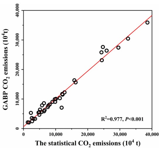
Figure 3.
Scatter plots of total CO2 emissions calculated from statistical energy consumption data and simulated CO2 emissions by GABP neural networks of three agglomerations in 2019.
The NPP/VIIRS nighttime light was used to allocate the city-level carbon emissions to 500 m pixel. Radiance values of all pixels belong to a region were summed, and the original value at each pixel was normalized by the regional sum. The CO2 emission intensity at a pixel was scaled by multiplying the normalized radiance with the annual total emissions of a country or a region [40]. Therefore, we obtained energy carbon emissions at 500 m resolution for three urban agglomerations in China from 2014 to 2019.
2.3.4. Spatiotemporal Dynamics of CO2 Emissions Based on GIS-Based Buffer Analysis, Kernel Density Estimation and Linear Regression Analysis
Kernel density estimation (KDE) is a nonparametric density estimation method to estimate the probability density of random variables. In this study, we used KDE to estimate the continuous probability density curves of carbon emissions to capture the kernel density maps of carbon emissions in three urban agglomerations [41].
The city areas in urban agglomerations adopted for the GIS-based buffer analysis were divided into three urbanization gradients. We designed two buffer zones around urban areas. Two kinds of buffer zones were established: first-level urban circle was the buffer zone with a width of 500 m outside the urban area, while second-level urban circle was the buffer zone with a width of 1 km outside the first-level urban circle [42]. Two circular buffer systems (first-level urban circle and second-level urban circle) were built by creating buffer zones to compare the characteristics of CO2 emissions between urban areas and sub-urban areas in urban agglomerations.
We calculated the variation slope (Sslope index) of energy consumption CO2 emissions from 2014 to 2019 by establishing linear regression model between CO2 emissions and years [43].
where n is the total number of years; xi is the serial number of year i; ti is the CO2 emission amount in the i year. When Sslope index was larger than 0, it meant that CO2 emissions showed an increasing trend. Significant trends of CO2 emissions in three urban agglomerations were divided into four levels. The first level was a high-decline region where Sslope was less than −0.16 and the second level was named as a low-decline region where Sslope was greater than −0.16 and less than 0. The third levels (0 < Sslope < 0.16) were named low-growth regions, and the last one (Sslope > 0.16) was called a high-growth region.
Profiles of CO2 emissions along urbanization gradients were investigated using the section line that passed through the city center. Cities with high CO2 emissions and low CO2 emissions were selected, respectively, in each urban agglomeration. We chose Beijing and Langfang in Beijing-Tianjin-Hebei, Shanghai and Chizhou in Yangtze River Delta, Guangzhou and Zhaoqing in Pearl River Delta as case studies.
2.3.5. Statistical Analysis on the Influencing Factors of CO2 Emissions among Urban Agglomerations
Population density, annual mean temperature and terrain slope excluding the predictors of the carbon emission model were selected as potential influencing factors of spatial pattern of CO2 emissions among urban agglomerations. First, population density was an important socioeconomic factor, which was often found to positively correlate with energy consumptions and CO2 emissions [44]. Second, climate was considered as a determinant of energy consumption and CO2 emissions due to heating and cooling [45,46]. Meanwhile, annual mean temperature was different among three urban agglomerations. Third, topography, for example, terrain slope, was a crucial natural factor because CO2 emissions of the car increased with the increase of terrain slope. In order to analyze the realistic factors affecting CO2 emissions, the strength of correlation between CO2 emissions and population density, annual mean temperature and terrain slope were estimated using the Pearson’s correlation coefficient. All influencing factors, such as population density, annual mean temperature and terrain slope, were resampled to 500 m resolution.
3. Results
3.1. Spatiotemporal Variations of CO2 Emissions
The spatial distribution of CO2 emissions appeared as different patterns in three urban agglomerations (Figure 4 and Figure 5). CO2 emissions in Beijing-Tianjin-Hebei Region presented a three-core distribution, such as Beijing, Tianjin and Tangshan. CO2 emissions in the Yangtze River Delta showed a multiple-core distribution, such as Nanjing, Zhenjiang, Wuxi, Suzhou, Shanghai and Ningbo. CO2 emissions in Pearl River Delta appeared as a null-core distribution (Figure 5).
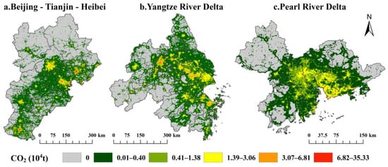
Figure 4.
Spatial distribution of annual CO2 emissions in three urban agglomerations averaged from 2014 to 2019.
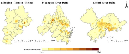
Figure 5.
Kernel density estimation maps of CO2 emissions of three urban agglomerations in 2019.
The Yangtze River Delta has the largest total CO2 emissions, followed by Beijing-Tianjin-Hebei region and the Pearl River Delta (Figure 6). CO2 emissions per unit in cities of the three agglomerations showed that the city with the lowest carbon emissions per unit in Beijing-Tianjin-Hebei was Langfang, while the highest was Tangshan. CO2 emissions per unit of Tangshan were 8.29 times that of Langfang. In the Yangtze River Delta, the city with the lowest carbon emissions per unit was Jinhua, while the highest was Maanshan. CO2 emissions per unit in Maanshan were 4.39 times that of Jinhua. In the Pearl River Delta, the city with the lowest carbon emissions per unit was Zhongshan, and the highest was Shenzhen. CO2 emissions per unit of Shenzhen was 2.46 times that of Zhongshan. Consequently, Beijing-Tianjin-Hebei Region have the largest variations in carbon emissions at city level, while the Pearl River Delta have the smallest variations.
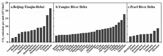
Figure 6.
CO2 emissions per unit in cities of three urban agglomerations.
Temporal patterns of CO2 emissions showed that th 28.74%, 43.99% and 43.45% of the areas appeared to have significant upward trends of CO2 emissions in Beijing-Tianjin-Hebei Region, Yangtze River Delta, and Pearl River Delta during 2014–2019, respectively (Figure 7). Meanwhile, the percentages of regions with significant downward trends of CO2 emissions were 15.43%, 13.47% and 15.31% in Beijing-Tianjin-Hebei, Yangtze River Delta, and Pearl River Delta during study period, respectively. In general, the areas with downward trends of carbon emissions were concentrated in southern Beijing, southern Tianjin, northern Tangshan, and western Handan in Beijing-Tianjin-Hebei, while these were dispersed in the Yangtze River Delta and Pearl River Delta. Moreover, the percentages of high-growth regions and low-growth regions in the upward trend regions were 2.88%, 5.46%, 3.44% and 4.75%, 3.97%, 2.22% in Beijing-Tianjin-Hebei, the Yangtze River Delta, and Pearl River Delta, respectively.
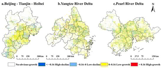
Figure 7.
Temporal trends of CO2 emissions in three urban agglomerations from 2014 to 2019. The white area was not passed the significance test (p > 0.05). High-decline: Sslope < −0.16; Low-decline: −0.16 < Sslope < 0; Low-growth: 0 < Sslope < 0.16; High-growth: 0.16 < Sslope.
3.2. Carbon Emissions within Cities
Urban areas have a larger amount of CO2 emissions than first-level urban circle and second-level urban circle (Figure 8a–c). In detail, the Sslope of carbon emissions in urban areas of the Yangtze River Delta was the largest, reaching 0.270, while that of Beijing-Tianjin-Hebei Region was the smallest, at only 0.018. The slopes of CO2 emissions in urban areas of Yangtze River Delta and Pearl River Delta were both larger than those in the other two urban circles.
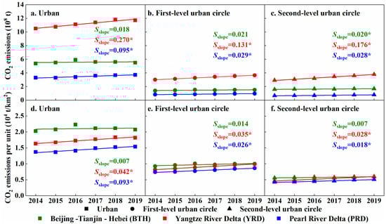
Figure 8.
CO2 emissions and CO2 emissions per unit within cities. The fitting curve indicated the temporal trend of CO2 emissions in three urban circles for each urban agglomeration and Sslope indicated the slope of energy CO2 emissions from 2014 to 2019. The star behind Sslope value mean the significance test of trend was passed (p < 0.05).
On the contrary, CO2 emissions per unit in urban areas, first-level urban circles and second-level urban circles in Beijing-Tianjin-Hebei were the highest among three urban agglomerations (Figure 8d–f). The temporal trends of CO2 emissions per unit in three urban circles of Yangtze River Delta and Pearl River Delta have increased significantly. The temporal slopes of CO2 emissions per unit in first-level urban circle and second-level urban circle of Yangtze River Delta were larger than that of Pearl River Delta, respectively (Figure 8d–f).
In order to further investigate the pattern of CO2 emissions along urbanization gradients, the section line that passed through the city center was used to obtain profile lines, which represented the structure of CO2 emissions along the distance away from urban centers. In this study, cities with high CO2 emissions and low CO2 emissions were selected respectively in each urban agglomeration (Figure 9). Profiles of CO2 emissions along urbanization gradients behaved as a radiation peak pattern with a high peak and a wide range in big cities (Figure 9a–c). Correspondingly, profiles of CO2 emissions showed an independent peak pattern with a low peak and a narrower range in small cities (Figure 9d–f).
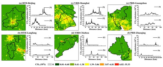
Figure 9.
Profiles of CO2 emissions along urbanization gradients in: (a) Beijing; (b) Langfang of Beijing-Tianjin-Hebei (BTH); (c) Shanghai; (d) Chizhou of Yangtze River Delta (YRD); (e) Guangzhou; and (f) Zhaoqing of Pearl River Delta (PRD).
3.3. Influencing Factors of Spatial Pattern of CO2 Emissions
Significant positive relationships between CO2 emissions and population density can be observed in each urban agglomeration (rBTH = 0.486; rYRD = 0.470; rPRD = 0.535; all p < 0.05) (Figure 10). Meanwhile, there were significant negative correlations between terrain slope and CO2 emissions in three agglomerations (rBTH = −0.178; rYRD = −0.156; rPRD = −0.335; all p < 0.05), which meant that CO2 emissions were generally decreasing when terrain slope increased. Furthermore, CO2 emissions have weak correlations with annual mean temperature in each agglomeration (rBTH = 0.172; rYRD = 0.004; rPRD = −0.124; all p < 0.05). It indicated that population density was the primary influencing factor of CO2 emissions in all urban agglomerations. Meanwhile, the Pearl River Delta was one of the three urban agglomerations which CO2 emissions most affected by terrain slope.
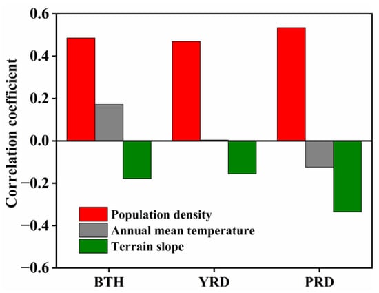
Figure 10.
Correlations between CO2 emissions and influencing factors, such as population density, annual mean temperature and terrain slope, in three major urban agglomerations. BTH: Beijing-Tianjin-Hebei; YRD: Yangtze River Delta; PRD: Pearl River Delta.
In general, there were significant positive correlations between carbon emissions and population density among three urban circles (Table 2), which indicated that CO2 emissions were increasing when population density increased. In detail, the correlations between CO2 emissions and population density in urban areas were more robust than other two urban circles, expect for Pearl River Delta, where CO2 emissions in second-level urban circle has largest correlations with population density. Meanwhile, CO2 emissions in urban areas of three urban agglomerations have the smallest correlation with the terrain slope, compared to other two urban circles. Additionally, temperature has the smallest impact on CO2 emissions (Table 2).
Table 2.
Relationships between CO2 emissions and population density, annual mean temperature and terrain slope among urban circles, such as urban area, first-level urban circle and second-level urban circle.
4. Discussion
4.1. NPP/VIIRS Nighttime Light Integrated Genetic Neural Network Showed a Good Performance in Estimating CO2 Emissions
Remote sensing nighttime light data can distinguish human urban areas with artificial lights from the dark background at night [14], and have a high correlation with the energy consumptions and carbon emissions [20]. One the one hand, the county-level statistical carbon emissions based on published energy use data were limited to coarse spatial/temporal resolution and short period [47]. Remote sensing nighttime light data were often selected as a good indicator to downscale the county-level statistical CO2 emissions [13,26]. Because the nighttime light data have wide time-span and coverage [48]. On the other hand, a range of methods, including linear regression model [26], power regression model [24] and log-log regression model [32] have been used in modeling spatiotemporal patterns of CO2 emissions based on nighttime light data and statistical energy consumption. However, traditional regression methods were not effective to track the nonlinear relationship between statistical CO2 emissions and nighttime light data due to fixed parameters [17]. Genetic neural networks have higher feasibility and reliability than traditional regression models. Jasiński (2019) modeled total electricity consumption based on nighttime light images with artificial neural networks, and found that the results achieved by artificial neural networks has higher precision than that using linear regressions [18]. For three northeastern provinces in China, Yang et al. (2020) found that the performance of a neural network model was superior to traditional regression models in analyzing the nonlinear relationship between nighttime light data and statistical carbon emissions [17]. For central and western regions of China, Lin et al. (2022) confirmed that a deep neural network ensemble model was the best method to establish the relationship between the multi-dimensional data characteristics and carbon emissions [49]. Our study demonstrated that genetic neural network can estimate the spatiotemporal patterns of CO2 emissions by integrating multiple datasets.
However, some limitations of nighttime light data will lead to uncertainty of CO2 emissions regardless of the linear function, power function or even complex methods. To a certain extent, over-estimation of CO2 emissions may exist in urban areas due to the limitation of nighttime light data. For example, some factories without any nighttime lights were likely to have intensive human activities and CO2 emissions during the day [50]. In general, the statistical carbon emissions consisted of whole urban CO2 emissions during the day and night. Many studies have reported that nighttime light data have a high correlation with energy consumptions and carbon emissions [17,35]. It indicated that brighter the nighttime lights, more daytime human activities in urban areas. For example, nighttime light data was commonly used as an indicator of overall energy use in urban, though electricity was often considered as the primary source of energy used for producing artificial light [51]. Therefore, remote sensing nighttime light data can still be considered as a good proxy of CO2 emissions in large-scale areas.
4.2. Three Urban Agglomerations Exhibited Diverse Spatial Patterns of CO2 Emissions
Beijing-Tianjin-Hebei Region behaved as three-core, Yangtze River Delta showed multiple-core and Pearl River Delta presented null-core structure in CO2 emissions, respectively (Figure 4 and Figure 5). The differential spatial patterns of CO2 emissions may be ascribed to various development modes in three urban agglomerations. Beijing-Tianjin-Hebei Region is one of China’s heavy industrial bases, which consists of a large number of high-energy-consuming enterprises, such as thermal power, steel and cement manufacturing. A Study indicated that energy was wasted in most cities in the Beijing-Tianjin-Hebei region [52]. Yangtze River Delta has low variations in urban development levels within agglomerations [53]. Shanghai, Zhejiang and Jiangsu Provinces in Yangtze River Delta could be classified as high development level regions, where CO2 emissions are relatively high and concentrated. As a hotspot for investment in the manufacturing industry, Pearl River Delta is making efforts on promoting green energy and building the national green development [54]. For example, cities like Shenzhen has witnessed great progress in cleaner production [55]. Therefore, diverse spatial patterns of carbon emissions among urban agglomerations reflected differences in socioeconomic structure.
4.3. Population Density Versus Terrain Slope Featured Opposite Effects on Spatial Pattern of CO2 Emissions
Positive relationships between population density and CO2 emissions while negative correlations between terrain slope and CO2 emissions were observed in three urban agglomerations (Figure 10). A study using STIRPAT model with panel data of China’s 30 provinces from 1997 to 2012 indicated that population size has a strong explanatory power on CO2 emissions [56]. The expansion of population scale directly leads to the extrusion of individual living space, posing a huge threat to population and environment [39]. Meanwhile, previous studies found that topographical factors were important limiting factors that influence population distribution and economic development [57]. Generally, the terrain of urban areas which less restricted the development of human activities is flat. But, in areas with complex terrain, such as mountainous areas and forest areas, human activities are greatly affected by slope, and the paving of roads and railways is also affected by natural environment. Therefore, inclination of terrain slope may decrease CO2 emissions. In addition, CO2 emissions decreased gradually with the increase of distance away from urban center in each urban agglomeration (Figure 8 and Figure 9). Decrease in effects of population density while increase in effects of terrain slope on CO2 emissions were found along the gradients from urban areas to first-level urban circles then to second-level urban circles (Table 2). So, differences in urban circles should be taken into consideration in formulating emission reduction policies.
5. Conclusions
Urban agglomerations, such as Beijing-Tianjin-Hebei, Yangtze River Delta and Pearl River Delta are the most developed regions in China, which are playing leadership roles in low-carbon development. We proposed a neural networks model based on nighttime light data to estimate CO2 emissions of three major urban agglomerations from 2014 to 2019. The results indicated that spatial distribution of CO2 emissions exhibited diversity among urban agglomerations. The areas appearing upward temporal trends of CO2 emissions were larger than that with downward temporal trends in each urban agglomeration. The total amount of CO2 emissions in the urban areas was largest among three urban circles, followed by first-level urban circle and second-level urban circle. In addition, population density had the greatest impact on spatial pattern of CO2 emissions, while temperature had the least impact. Urban agglomerations should coordinate development strategies in economic growth versus carbon reduction.
Author Contributions
Conceptualization, L.Z., J.S. and Y.C.; Methodology, L.Z., J.S. and Y.C.; Formal analysis, L.Z. and J.S; Writing-original draft, L.Z. and J.S.; Writing–review & editing, L.Z., Y.C. and Q.Y.; Supervision, Y.C.; funding acquisition, Y.C. All authors have read and agreed to the published version of the manuscript.
Funding
This research was funded by National Natural Science Foundation of China (41871084), National Key Research and Development Program of China (2017YFB0504000), Soft Science Research Program of Zhejiang Provincial Department of Science and Technology (2022C35095), Jinhua Science and Technology Research Program (2021-4-340 and 2020-4-184), and Self-Design Project in Zhejiang Normal University (2021ZS07).
Data Availability Statement
The multi-source data used in this paper are publicly available, and the dataset information is shown in Table 1.
Conflicts of Interest
The authors declare no conflict of interest.
References
- Pablo-Romero, M.d.P.; Pozo-Barajas, R.; Yñiguez, R. Global changes in residential energy consumption. Energy Policy 2017, 101, 342–352. [Google Scholar] [CrossRef]
- Zheng, J.; Dong, S.; Hu, Y.; Li, Y. Comparative analysis of the CO2 emissions of expressway and arterial road traffic: A case in Beijing. PLoS ONE 2020, 15, e0231536. [Google Scholar] [CrossRef] [PubMed]
- Shi, K.; Yu, B.; Zhou, Y.; Chen, Y.; Yang, C.; Chen, Z.; Wu, J. Spatiotemporal variations of CO2 emissions and their impact factors in China: A comparative analysis between the provincial and prefectural levels. Appl. Energy 2019, 233–234, 170–181. [Google Scholar] [CrossRef]
- Zhou, D.; Zhao, S.; Liu, S.; Zhang, L.; Zhu, C. Surface urban heat island in China’s 32 major cities: Spatial patterns and drivers. Remote Sens. Environ. 2014, 152, 51–61. [Google Scholar] [CrossRef]
- Grimm, N.B.; Faeth, S.H.; Golubiewski, N.E.; Redman, C.L.; Wu, J.; Bai, X.; Briggs, J.M. Global change and the ecology of cities. Science 2008, 319, 756–760. [Google Scholar] [CrossRef]
- Dong, F.; Yu, B.; Hadachin, T.; Dai, Y.; Wang, Y.; Zhang, S.; Long, R. Drivers of carbon emission intensity change in China. Resour. Conserv. Recycl. 2018, 129, 187–201. [Google Scholar] [CrossRef]
- Yu, X.; Wu, Z.Y.; Zheng, H.R.; Li, M.Q.; Tan, T.L. How urban agglomeration improve the emission efficiency? A spatial econometric analysis of the Yangtze river delta urban agglomeration in China. J. Environ. Manag. 2020, 263, 110061. [Google Scholar] [CrossRef]
- Chen, J.; Gao, M.; Cheng, S.; Liu, X.; Hou, W.; Song, M.; Li, D.; Fan, W. China’s city-level carbon emissions during 1992–2017 based on the inter-calibration of nighttime light data. Sci. Rep. 2021, 11, 3323. [Google Scholar] [CrossRef]
- Cai, B.; Zhang, L. Urban CO2 emissions in China: Spatial boundary and performance comparison. Energy Policy 2014, 66, 557–567. [Google Scholar] [CrossRef]
- Dhakal, S. Urban energy use and carbon emissions from cities in China and policy implications. Energy Policy 2009, 37, 4208–4219. [Google Scholar] [CrossRef]
- Sheng, Y.; Miao, Y.; Song, J.; Shen, H. The Moderating Effect of innovation on the relationship between urbanization and CO2 emissions: Evidence from three major urban agglomerations in China. Sustainability 2019, 11, 1633. [Google Scholar] [CrossRef]
- Sheng, P.; Guo, X. The long-run and short-run impacts of urbanization on carbon dioxide emissions. Econ. Model. 2016, 53, 208–215. [Google Scholar] [CrossRef]
- Shi, K.; Chen, Y.; Li, L.; Huang, C. Spatiotemporal variations of urban CO2 emissions in China: A multiscale perspective. Appl. Energy 2018, 211, 218–229. [Google Scholar] [CrossRef]
- Elvidge, C.D.; Baugh, K.E.; Kihn, E.A.; Kroehl, H.W.; Davis, E.R.; Davis, C.W. Relation between satellite observed visible-near infrared emissions, population, economic activity and electric power consumption. Int. J. Remote Sens. 1997, 18, 1373–1379. [Google Scholar] [CrossRef]
- Oda, T.; Maksyutov, S.; Elvidge, C.D. Disaggregation of national fossil fuel CO2 emissions using a global power plant database and DMSP nightlight data. Proc. Asia-Pac. Adv. Netw. 2010, 30, 219–228. [Google Scholar] [CrossRef]
- Ou, J.; Liu, X.; Li, X.; Li, M.; Li, W. Evaluation of NPP-VIIRS Nighttime Light Data for Mapping Global Fossil Fuel Combustion CO2 Emissions: A Comparison with DMSP-OLS Nighttime Light Data. PLoS ONE 2015, 10, e0138310. [Google Scholar] [CrossRef] [PubMed]
- Yang, D.; Luan, W.; Qiao, L.; Pratama, M. Modeling and spatio-temporal analysis of city-level carbon emissions based on nighttime light satellite imagery. Appl. Energy 2020, 268, 114696. [Google Scholar] [CrossRef]
- Jasiński, T. Modeling electricity consumption using nighttime light images and artificial neural networks. Energy 2019, 179, 831–842. [Google Scholar] [CrossRef]
- Li, H.; Zhao, Y.; Qiao, X.; Liu, Y.; Cao, Y.; Li, Y.; Wang, S.; Zhang, Z.; Zhang, Y.; Weng, J. Identifying the driving forces of national and regional CO2 emissions in China: Based on temporal and spatial decomposition analysis models. Energy Econ. 2017, 68, 522–538. [Google Scholar] [CrossRef]
- Mi, Z.; Zheng, J.; Meng, J.; Zheng, H.; Li, X.; Coffman, D.M.; Woltjer, J.; Wang, S.; Guan, D. Carbon emissions of cities from a consumption-based perspective. Appl. Energy 2019, 235, 509–518. [Google Scholar] [CrossRef]
- Chen, L.; Xu, L.; Cai, Y.; Yang, Z. Spatiotemporal patterns of industrial carbon emissions at the city level. Resour. Conserv. Recycl. 2021, 169, 105499. [Google Scholar] [CrossRef]
- Doll, C.H.; Muller, J.P.; Elvidge, C.D. Night-time imagery as a tool for global mapping of socioeconomic parameters and greenhouse gas emissions. AMBIO 2000, 29, 157–162. [Google Scholar] [CrossRef]
- Wang, S.; Liu, X. China’s city-level energy-related CO2 emissions: Spatiotemporal patterns and driving forces. Appl. Energy 2017, 200, 204–214. [Google Scholar] [CrossRef]
- Shi, K.; Chen, Z.; Cui, Y.; Wu, J.; Yu, B. NPP-VIIRS nighttime light data have different correlated relationships with fossil fuel combustion carbon emissions from different sectors. IEEE Geosci. Remote Sens. Lett. 2020, 18, 2062–2066. [Google Scholar] [CrossRef]
- Zhao, J.; Chen, Y.; Ji, G.; Wang, Z. Residential carbon dioxide emissions at the urban scale for county-level cities in China: A comparative study of nighttime light data. J. Clean. Prod. 2018, 180, 198–209. [Google Scholar] [CrossRef]
- Shi, K.; Yu, B.; Huang, Y.; Hu, Y.; Yin, B.; Chen, Z.; Chen, L.; Wu, J. Evaluating the ability of NPP-VIIRS nighttime light data to estimate the gross domestic product and the electric power consumption of China at multiple scales: A comparison with DMSP-OLS data. Remote Sens. 2014, 6, 1705–1724. [Google Scholar] [CrossRef]
- Sun, T.; Sun, R.; Khan, M.S.; Chen, L. Urbanization increased annual precipitation in temperate climate zone: A case in Beijing-Tianjin-Hebei region of North China. Ecol. Indic. 2021, 126, 107621. [Google Scholar] [CrossRef]
- Chen, L.; Liu, M.; Xu, Z.; Fan, R.; Tao, J.; Chen, D.; Zhang, D.; Xie, D.; Sun, J. Variation trends and influencing factors of total gaseous mercury in the Pearl River Delta—A highly industrialised region in South China influenced by seasonal monsoons. Atmos. Environ. 2013, 77, 757–766. [Google Scholar] [CrossRef]
- Ye, Y.; Zhang, H.; Liu, K.; Wu, Q. Research on the influence of site factors on the expansion of construction land in the Pearl River Delta, China: By using GIS and remote sensing. Int. J. Appl. Earth Obs. Geoinf. 2013, 21, 366–373. [Google Scholar] [CrossRef]
- Song, Y.; Long, Y.; Wu, P.; Wang, X. Are all cities with similar urban form or not? Redefining cities with ubiquitous points of interest and evaluating them with indicators at city and block levels in China. Int. J. Geogr. Inf. Sci. 2018, 32, 2447–2476. [Google Scholar] [CrossRef]
- Zhang, W.; Cui, Y.; Wang, J.; Wang, C.; Streets, D.G. How does urbanization affect CO2 emissions of central heating systems in China? An assessment of natural gas transition policy based on nighttime light data. J. Clean. Prod. 2020, 276, 123188. [Google Scholar] [CrossRef]
- Shi, K.; Yu, B.; Hu, Y.; Huang, C.; Chen, Y.; Huang, Y.; Chen, Z.; Wu, J. Modeling and mapping total freight traffic in China using NPP-VIIRS nighttime light composite data. GISci. Remote Sens. 2015, 52, 274–289. [Google Scholar] [CrossRef]
- Liu, H.; Ma, L.; Xu, L. Estimating spatiotemporal dynamics of county-level fossil fuel consumption based on integrated nighttime light data. J. Clean. Prod. 2021, 278, 123427. [Google Scholar] [CrossRef]
- Bennett, M.M.; Smith, L.C. Advances in using multitemporal night-time lights satellite imagery to detect, estimate, and monitor socioeconomic dynamics. Remote Sens. Environ. 2017, 192, 176–197. [Google Scholar] [CrossRef]
- Su, Y.; Chen, X.; Li, Y.; Liao, J.; Ye, Y.; Zhang, H.; Huang, N.; Kuang, Y. China’s 19-year city-level carbon emissions of energy consumptions, driving forces and regionalized mitigation guidelines. Renew. Sustain. Energy Rev. 2014, 35, 231–243. [Google Scholar] [CrossRef]
- Fang, C.; Wang, S.; Li, G. Changing urban forms and carbon dioxide emissions in China: A case study of 30 provincial capital cities. Appl. Energy 2015, 158, 519–531. [Google Scholar] [CrossRef]
- Rumelhart, D.E.; Hinton, G.E.; Williams, R.J. Learning Internal Representations by Error Propagation; California University San Diego, Institute for Cognitive Science: La Jolla, CA, USA, 1985. [Google Scholar]
- Yu, L.; He, Y. Evaluation of sports training effect based on GABP neural network and artificial intelligence. J. Ambient. Intell. Humaniz. Comput. 2021, 1–11. [Google Scholar] [CrossRef]
- Wang, P.; Wu, W.; Zhu, B.; Wei, Y. Examining the impact factors of energy-related CO2 emissions using the STIRPAT model in Guangdong Province, China. Appl Energy 2013, 106, 65–71. [Google Scholar] [CrossRef]
- Oda, T.; Maksyutov, S. A very high-resolution (1 km × 1 km) global fossil fuel CO2 emission inventory derived using a point source database and satellite observations of nighttime lights. Atmos. Chem. Phys. 2011, 11, 543–556. [Google Scholar] [CrossRef]
- Ke, N.; Lu, X.; Zhang, X.; Kuang, B.; Zhang, Y. Urban land use carbon emission intensity in China under the “double carbon” targets: Spatiotemporal patterns and evolution trend. Environ. Sci. Pollut. Res. Int. 2022, 1–14. [Google Scholar] [CrossRef]
- Li, X.; Zhang, L.; Liang, C. A GIS-based buffer gradient analysis on spatiotemporal dynamics of urban expansion in Shanghai and its major satellite cities. Procedia Environ. Sci. 2010, 2, 1139–1156. [Google Scholar] [CrossRef]
- He, C.; Ma, Q.; Li, T.; Yang, Y.; Liu, Z. Spatiotemporal dynamics of electric power consumption in Chinese Mainland from 1995 to 2008 modeled using DMSP/OLS stable nighttime lights data. J. Geogr. Sci. 2012, 22, 125–136. [Google Scholar] [CrossRef]
- Puliafito, S.E.; Puliafito, J.L.; Grand, M.C. Modeling population dynamics and economic growth as competing species: An application to CO2 global emissions. Ecol. Econ. 2008, 65, 602–615. [Google Scholar] [CrossRef]
- Nie, H.G.; Kemp, R.; Xu, J.H.; Vasseur, V.; Fan, Y. Drivers of urban and rural residential energy consumption in China from the perspectives of climate and economic effects. J. Clean. Prod. 2018, 172, 2954–2963. [Google Scholar] [CrossRef]
- Zhu, D.; Tao, S.; Wang, R.; Shen, H.; Huang, Y.; Shen, G.; Wang, B.; Li, W.; Zhang, Y.; Chen, H.; et al. Temporal and spatial trends of residential energy consumption and air pollutant emissions in China. Appl. Energy 2013, 106, 17–24. [Google Scholar] [CrossRef]
- Guan, D.; Liu, Z.; Geng, Y.; Lindner, S.; Hubacek, K. The gigatonne gap in China’s carbon dioxide inventories. Nat. Clim. Chang. 2012, 2, 672–675. [Google Scholar] [CrossRef]
- Chen, J.; Gao, M.; Cheng, S.; Hou, W.; Song, M.; Liu, X.; Liu, Y.; Shan, Y. County-level CO2 emissions and sequestration in China during 1997–2017. Sci. Data 2020, 7, 391. [Google Scholar] [CrossRef]
- Lin, X.; Ma, J.; Chen, H.; Shen, F.; Ahmad, S.; Li, Z. Carbon emissions estimation and spatiotemporal analysis of china at city level based on multi-dimensional data and machine learning. Remote Sens. 2022, 14, 3014. [Google Scholar] [CrossRef]
- Zhao, N.; Samson, E.L.; Currit, N.A. Nighttime-lights-derived fossil fuel carbon dioxide emission maps and their limitations. Photogramm. Eng. Remote Sens. 2015, 81, 935–943. [Google Scholar] [CrossRef]
- Mellander, C.; Lobo, J.; Stolarick, K.; Matheson, Z. Night-time light data: A good proxy measure for economic activity? PloS ONE 2015, 10, e0139779. [Google Scholar] [CrossRef]
- Sun, J.; Wang, Z.; Zhu, Q. Analysis of resource allocation and environmental performance in China’s three major urban agglomerations. Environ. Sci. Pollut. Res. Int. 2020, 27, 34289–34299. [Google Scholar] [CrossRef] [PubMed]
- Zhou, Y.; Chen, M.X.; Tang, Z.P.; Mei, Z.A. Urbanization, land use change, and carbon emissions: Quantitative assessments for city-level carbon emissions in Beijing-Tianjin-Hebei region. Sustain. Cities Soc. 2021, 66, 102701. [Google Scholar] [CrossRef]
- Wang, M.X.; Zhao, H.H.; Cui, J.X.; Fan, D.; Lv, B.; Wang, G.; Li, Z.H.; Zhou, G.J. Evaluating green development level of nine cities within the Pearl River Delta, China. J. Clean. Prod. 2018, 174, 315–323. [Google Scholar] [CrossRef]
- Wang, S.J.; Zeng, J.Y.; Huang, Y.Y.; Shi, C.Y.; Zhan, P.Y. The effects of urbanization on CO2 emissions in the Pearl River Delta: A comprehensive assessment and panel data analysis. Appl. Energy 2018, 228, 1693–1706. [Google Scholar] [CrossRef]
- Wang, Y.A.; Kang, Y.Q.; Wang, J.; Xu, L.N. Panel estimation for the impacts of population-related factors on CO2 emissions: A regional analysis in China. Ecol. Indic. 2017, 78, 322–330. [Google Scholar] [CrossRef]
- Zhang, J.J.; Zhu, W.B.; Zhu, L.Q.; Cui, Y.P.; He, S.S.; Ren, H. Topographical relief characteristics and its impact on population and economy: A case study of the mountainous area in western Henan, China. J. Geogr. Sci. 2019, 29, 598–612. [Google Scholar] [CrossRef]
Disclaimer/Publisher’s Note: The statements, opinions and data contained in all publications are solely those of the individual author(s) and contributor(s) and not of MDPI and/or the editor(s). MDPI and/or the editor(s) disclaim responsibility for any injury to people or property resulting from any ideas, methods, instructions or products referred to in the content. |
© 2023 by the authors. Licensee MDPI, Basel, Switzerland. This article is an open access article distributed under the terms and conditions of the Creative Commons Attribution (CC BY) license (https://creativecommons.org/licenses/by/4.0/).