Abstract
Land degradation threatens ecosystems and socio-economic development of Southern Africa. Evaluation of land degradation is widely conducted using a remote-sensed indicator to provide key information for alleviating degradation. However, the commonly used single indicator cannot reveal complex degradation processes. In this study, we conducted an integrated evaluation by utilizing linear regression, residual trend analysis, and sequential regression methods to detect visible, potential human-induced, and functional land degradation in Southern Africa. The results showed that visible, potential, and functional land degradation accounted for 8%, 9.6%, and 21.9% of the entire study area, respectively. In total, 34% (171.96 × 10⁴ km2) of the region exhibited one or more forms of land degradation; 28.9% (146.01 × 10⁴ km2) of the land experienced a single land degradation type, whereas 5.1% (25.95 × 10⁴ km2) exhibited intensified degradation by two or three forms. Land degradation was more severe in South Africa, Angola, Botswana, and Mozambique. Potential degradation (11.76%) and functional degradation (56.88%) may co-exist with vegetation greening. This study suggests that a single indicator assessment underestimates the overall land degradation, and thus integrated indicators and methods are better for a comprehensive assessment. Spatial pattern and degradation process analyses are useful for the formulation of land restoration policies in Southern Africa.
1. Introduction
Land degradation is defined as a persistent decline in ecosystem productivity as well as a reduction in ecosystem resilience caused by climate change and human activities [1]. Degradation prevents land from providing important ecosystem services, such as water, food and timber supply, and carbon sequestration, and may exacerbate environmental degradation, resulting in poverty [2]. Land degradation mainly affects drylands, which account for 41% of the global land area and support about 50% of global livestock and 38% of the global human population [3,4]. Therefore, it is imperative to detect the extent and intensity of land degradation in drylands to improve our understanding of degradation processes and formulate strategies for sustainable land management [5,6,7].
Southern Africa includes 10 countries: Angola (AGO), Zambia (ZMB), Zimbabwe (ZWE), Malawi (MWI), Mozambique (MOZ), Namibia (NAM), Botswana (BWA), South Africa (ZAF), Lesotho (LSO), and the Republic of Eswatini (EW). These countries are undeveloped compared to other regions of the world [2]. Approximately 85% of the area in Southern Africa is classified as drylands according to the definition of aridity by the Food and Agriculture Organization [8]. The proportion is predicted to increase with global warming and increase in aridity, making more people and ecosystems vulnerable to water scarcity, as well as causing desertification and loss of livelihoods [9,10]. Factors that promote land degradation in the region include deforestation [11], harvesting of natural resources [12], and soil erosion [13,14]. In addition, human activities such as urbanization and agriculture expansion have accelerated land degradation in this region. Therefore, detection of land degradation is valuable for countries in Southern Africa in evaluating the effectiveness of environmental protection policy and to predict potential environmental destruction.
The variability of vegetation is driven by the combined effects of climate, human activities, and sensitivity of vegetation response [15,16,17]. Three vegetation-derived indicators are commonly used to detect land degradation: visible land degradation (the decreased linear trend of vegetation greenness) [18], human-induced potential land degradation (the decrease in the residual of the vegetation–rainfall relationship) [19,20], and functional land degradation (the decrease in the sensitivity of vegetation to rainfall) [21,22]. Visible land degradation is represented by a decline in vegetation greenness that can be visually observed in field surveys or remote sensing images [18]. An increase or decrease in the Normalized Difference Vegetation Index (NDVI) indicates visible land improvement or degradation, respectively [18]. Human-induced potential land degradation is commonly assessed through Residual Trend (RESTREND) and Time Series Segmentation and Residual Trend (TSS-RESTREND) analyses [23,24]. These two methods exclude the impacts of climate variables such as rainfall on the vegetation variability and attribute vegetation degradation to human activities [20]. The RESTREND method can more accurately reflect human-induced degradation than linear trend measures of vegetation indices [19,25,26]. Functional land degradation is usually represented by a decrease in the sensitivity of vegetation to rainfall (SVR) [27]. SVR represents the function of precipitation utilization by the ecosystem. SVR decreases with an increase in environmental deterioration. Previous findings indicate that shrub encroachment decreases the proportion of grasses and induces decreases in SVR [28]. Each of the three indicators is mainly used to represent a specific aspect of land degradation. However, most of the actual land degradation is not a single process, and these three types of dynamics of degradation assessment indices (visible, potential, and functional land degradation) may coexist in the same region [29,30,31,32,33], so a single assessment does not reflect the reality. An integrated land degradation assessment system is required that includes all the three indicators to have a comprehensive understanding of land degradation.
Previous studies have reported that land degradation is widely multifaceted [34]. Global greening has been observed despite the constantly increasing aridity [29]. This indicates the decoupling between ecosystem function and its optical reflectance [35]. The increase in vegetation greenness may also be caused by land degradation-related processes, such as shrub encroachment caused by overgrazing and drought [30]. Multiple degradations can be attributed to the same factors and integrated land degradation processes. For instance, deforestation-induced degradation of function and structure is related with cropland extension, which require differentiated indicators to characterize [36,37]. Therefore, the detection of land degradation should be conducted using multiple indicators.
The hypothesis of this study was that land degradation caused by climate, human activities, and ecosystem functional change varies in different regions in Southern Africa. This hypothesis was tested by evaluating three types of land degradation, including visible land degradation, human-induced potential land degradation, and functional land degradation. The specific objectives of this study were (1) to evaluate the spatial patterns of three types of land degradation in Southern Africa, and (2) to investigate whether the three indicators for land degradation assessment help to detect and provide comprehensive information on land degradation processes. The time scales and parameters for the evaluation of the three indicators were aligned to enable the comparison of different land degradation types.
2. Materials and Methods
2.1. Study Area
Southern Africa is composed of 10 countries (Figure 1a). The annual rainfall in most of Southern Africa is below 1000 mm, the aridity index is below 0.65 (Figure 1c,d), and the vegetation growth is mainly limited by rainfall [38]. Annual rainfall in the study area gradually decreases from the northeast to the southwest, and the land cover changes from forest in the northeast to shrubs and bare land in the southwest [39] (Figure 1b). Increases in population in the study area have increased the demand for food, water, and timber for the construction of infrastructure, which has been met by expanding and intensifying agricultural activities, grazing, groundwater extraction, and timber harvesting [12].
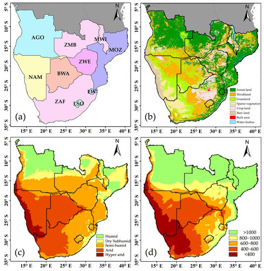
Figure 1.
(a) A map showing the boundaries of different countries: Angola (AGO), Zambia (ZMB), Zimbabwe (ZWE), Malawi (MWI), Mozambique (MOZ), Namibia (NAM), Botswana (BWA), South Africa (ZAF), Lesotho (LSO), and the Republic of Eswatini (EW); (b) land cover in Southern Africa derived from [39]; (c) dryland cover in Southern Africa based on the aridity index, with hyper-arid (<0.05), arid (0.05–0.2), semi-arid (0.2–0.5), and dry sub-humid (0.5–0.65) classifications and (d) annual precipitation (mm).
2.2. Dataset Source
2.2.1. Vegetation Index
The Global Inventory Monitoring and Modeling System (GIMMS) NDVI dataset obtained from 1981 to 2015 with a semi-monthly temporal resolution and a 0.0833° spatial resolution was used in this study. The GIMMSv3.1g dataset was obtained from the U.S. National Aeronautics and Space Agency [40] (https://ecocast.arc.nasa.gov/data/pub/gimms/, accessed on 1 August 2019). A region with a mean NDVI below 0.1 cannot represent the real vegetation status, owing to the impact of the reflectance of soil on the vegetation index; thus, these areas were excluded from the analysis [35]. NDVI values were resampled using the principle of first-order conservation remapping in R from 1/12° to 0.1° to match the resolution of the rainfall data, and the monthly NDVI was derived from the mean semi-monthly values. The annual NDVI was obtained from the maximum value of the monthly NDVI from October to September of the subsequent year (for example, 1982/10 to 1983/10), which included the growing season in the southern hemisphere.
2.2.2. Rainfall
The Multi-Source Weighted-Ensemble Precipitation (MSWEP) V2 dataset (1979–2017) with a monthly temporal resolution and a 0.1° spatial resolution was used in this study [41]. The dataset was derived by optimally merging the range of the gauge, satellite, and reanalysis estimates. The MSEWP V2 dataset from 1980 to 2015 is available online (http://www.gloh2o.org/, accessed on 1 August 2019). Compared with other datasets, MSWEP has been shown to perform better in long-term mean rainfall estimates for global, land, and ocean domains [37] and has a relatively higher spatial resolution than datasets such as Climate Research Unit (CRU) and Global Precipitation Climatology Centre (GPCC) [42]. Vegetation dynamics are related to long-term precipitation, implying that vegetation may respond to previous rainfall. This is described as the lag effect and can be represented with two parameters: the offset period, and the accumulated period [15,43]. Thus, the offset (0–3 months) and accumulation effect (1–12 months) were included in the calculation. The optimal accumulated rainfall corresponds to the most significant vegetation and precipitation relationship.
2.2.3. Land Cover
Global Land Cover 2000 (GLC 2000) was generated with a 1 km spatial resolution with data from four sensors onboard Earth-observing satellites, with each source selected to map a specific ecosystem or land cover, seasonality, or water regime. GLC2000 was generated by regional experts to incorporate the experience of local knowledge in the mapping process, and each continent was mapped independently [39]. This procedure ensured that the optimum image classification methods were used, and that the land cover legend was regionally representative [39]. The validation of the GLC2000 regional products based on a comparison with different reference datasets shows a high degree of credibility for the GLC 2000 [39]. The land cover map of Africa used in this study can be obtained from the Joint Research Centre through the Global Vegetation Monitoring Unit (https://www.gvm.jrc.it/glc2000/ProductGLC2000.htm, accessed on 1 August 2019). The first level includes 7 land cover types (forests, woodlands and shrublands, grasslands, agricultural lands, bare soils, and other land-cover classes), and the second level includes 27 classes. The following land-cover classes were used: forest land (including the different tree covers shown in Figure 1), shrubland, grassland, sparse vegetation area (sparse herbaceous and sparse shrubs), cropland (cultivated areas), and bare land.
2.3. Methods
The linear trend analysis, TSS-RESTREND, and Sequential Regression (SeRGS) analysis were used to detect visible, potential, and functional land degradation (Figure 2). The annual maximum NDVI and accumulated rainfall were derived from monthly NDVI and rainfall time series. The optimal accumulated rainfall and annual maximum NDVI were regressed to obtain residual and SVR in TSS-RESTREND and SeRGS methods. Annual maximum NDVI was regressed with time to determine the trend of NDVI for visible land degradation. The indices used in these three assessments were unified to enable comparisons of land degradation from multiple aspects.
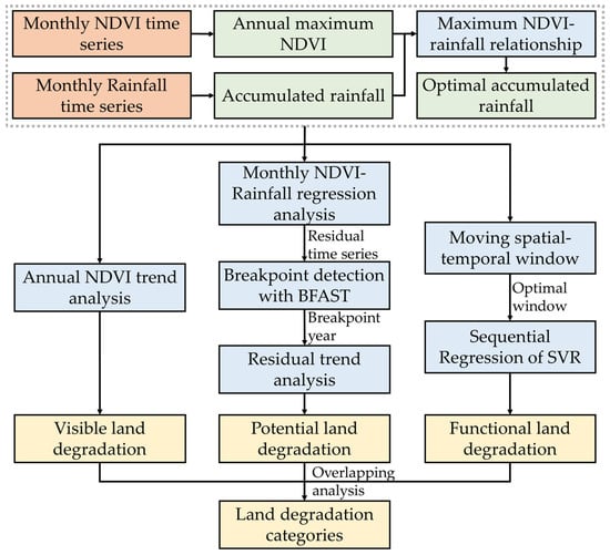
Figure 2.
Flowchart of methods. Abbreviations: NDVI, Normalized Difference Vegetation Index; BFAST, Breaks for Additive Seasonal and Trend; SVR, sensitivity of vegetation to rainfall.
2.3.1. Raw NDVI Trends
The NDVI trend is attributed to the dynamics in rainfall, SVR (vegetation function), and residual factor (human activity) [19]. The linear regression of annual maximum NDVI over time was conducted using the “lm” package in R [44], and the confidence level was set at 90% (p < 0.1).
2.3.2. Time Series Segmented and Residual Trend Analysis (TSS-RESTREND)
The TSS-RESTREND method optimizes the results of the RESTREND analysis by including a step of Breaks for Additive Seasonal and Trend (BFAST) analysis [23]. Firstly, regression analysis of the monthly vegetation index and accumulated rainfall was performed to obtain the monthly residual series. The breakpoint of the residual series was determined using the BFAST method [45], and the significance was verified with the Chow test (p < 0.05) [46]. A linear regression between the annual maximum NDVI and optimal accumulated rainfall was conducted for non-significant breakpoints based on Equation (1) (p < 0.1). For the significant breakpoints, RESTREND analysis was divided into two separate phases to eliminate the effect of SVR changes on the RESTREND calculation. The significant breakpoints were incorporated into the piecewise linear regression between the annual NDVI and the corresponding optimal rainfall, and the residual trend was calculated with two parts of the residual time series. The sum of residual change and VPR break height is the value of total change in TSS-RESTREND.
The results can be divided into five classes (Segmented SVR, Segmented Residual, RESTREND, Insignificant SVR, and Negative SVR) depending on whether the breakpoints and regression are significant [23]. Insignificant SVR and Negative SVR indicate that the TSS-RESTREND method is not suitable for application in these areas. The first three types provide the value of the cumulative changes in residuals and intercepts. Therefore, the detected potential land degradation is derived from the negative value of the first three types [23]. TSS-RESTREND analysis was conducted with the package “TSS.RESTREND” in R (https://cran.r-project.org/src/contrib/TSS.RESTREND_0.3.1.tar.gz, accessed on 1 August 2019).
2.3.3. Sequential Regression (SeRGS) Analysis of the Trend of Sensitivity of Vegetation to Rainfall (SVR)
SVR is the slope of the regression between NDVI and rainfall (Equation (1)). Sequential Regressions (SeRGs) can be applied in a moving window to determine the sequential dynamics of SVR. The moving window includes a spatial dimension (1, 3, 5, and 7 pixels) and a temporal dimension (5, 10, 15, 20, 25, and 30 years). The proportion of significant SVR (p < 0.1) was calculated for each spatial and temporal window. A linear regression of SVR over time at a corresponding pixel can only be conducted when the SVR in all temporal windows is significant [47]. The criteria for selecting the optimal spatial–temporal window combination include obtaining the largest possible proportion of significant vegetation precipitation relationships in the smallest possible temporal and spatial windows [47]. The proportion of significant SVR increased with increases in the size of the spatial–temporal windows (Figure S2). In this study, the optimal spatial and temporal windows were 3 pixels and 15 years, respectively. Therefore, there were 20 SVR pairs at each spatial window, and the significance (p < 0.1) of every SVR was a prerequisite for the calculation of the SVR trend (Figure S1b). SVR could be regressed over time in R with package “lm” [44], and the significantly (p < 0.1) negative SVR trend was used as the functional land degradation.
2.3.4. Overlay of Land Degradation Assessment
The spatial maps of visible, potential, and functional land degradation assessments were overlaid to determine the relationship between the three indicators and to evaluate the degradation of the study area. The land degradation overlay can be divided into 8 categories depending on whether the specific land degradation exists (Table 1). Category A represents entirely undegraded land; category B, C, and D represent visible, potential, and functional land degradation, respectively, without the other types of land degradation; category E, F, and G represent the co-occurrence of two types of land degradation, as shown in Table 1; category H represents the co-occurrence of the three types of land degradation.

Table 1.
The overlay of land degradation assessment. Existing land degradation is indicated with a red circle; green circles indicate no significant changes in indicators or significant increases in corresponding indices.
2.3.5. Retrieval of Land Degradation Datasets from Previous Studies
The cases related to land degradation types, spatial patterns, drivers, and processes in Southern Africa were retrieved from previous studies. The case data of land degradation were geographically aligned and digitized with ArcGIS 10.6, including point, line, and surface elements The obtained data were used to perform a qualitative analysis by overlaying them into the degradation results for spatial comparison. The relevant literature was reviewed, and the drivers and processes of land degradation are presented as a table. The spatial extent of land degradation cases was digitized for analysis of the results of this study.
3. Results
3.1. Spatial Patterns of Visible, Potential, and Functional Land Degradation
The three types of land degradation determined in this study are presented in Figure 3. The areas with no changes had the highest proportion, which were 45.9%, 61.2%, and 55.9% for the visible, potential, and functional land degradation, respectively. The proportions of increasing trend determined by all three methods were higher than the proportions of land degradation. Visible land degradation accounted for 8% of the study area, mainly in the north-eastern and north-western parts of the study area (Figure 3a). The increasing NDVI accounted for 46.2% of the study area and was mainly distributed in the central, southern, and western regions. The types of techniques in TSS-RESTREND are shown in Figure S1a. Areas with potential land degradation and improvement accounted for 9.6% and 29.2% of the study area, respectively (Figure 3b). Potential land degradation was mainly distributed in the west, southwest, and east of the study area (including south-western Angola, western South Africa, northern Namibia, south-eastern Zimbabwe, and Mozambique) (Figure 3b). Areas with functional land degradation and improvement accounted for 21.9% and 22.2% of the study area, respectively (Figure 3c). Functional land degradation was mainly observed in the central and south regions of the study area (including Botswana, South Africa, central Namibia, southwestern Zimbabwe, and southern Mozambique) (Figure 3c).
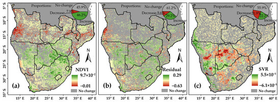
Figure 3.
Spatial pattern of (a) visible land degradation (yr−1), (b) potential land degradation (yr−1), and (c) functional land degradation (mm−1 yr−1). Only significant (p < 0.1) land degradation (red) and improvement (green) are displayed. Grey areas indicate non-significant changes. The inset pie charts indicate the proportions of decrease (red), increase (green), and no significant change (grey).
The three types of land degradation detected in this study were overlapped to obtain the combination of land degradation (Figure 4). The proportion of areas with land degradation was 34% (including categories B, C, D, E, F, G, H). Category D (functional land degradation) was the most widely distributed (19.8%, 99.86 × 10⁴ km2), followed by C (potential land degradation) (5.1%, 25.77 × 10⁴ km2) and B (visible land degradation) (4.0%, 20.38 × 10⁴ km2); category E included the co-occurrence of visible land degradation and potential land degradation with a proportion of 3.0% (15.05 × 10⁴ km2). The proportion of area covered by one type of land degradation (Situations B, C, and D) was 28.9% (146.01 × 10⁴ km2), whereas the proportion of area presenting with two or three types of land degradations (categories E, F, G, and H) was 5.1% (25.95 × 10⁴ km2). South Africa, Angola, and Namibia had the largest total areas of land degradation, and Botswana, Zimbabwe, and South Africa had the largest proportions of areas under land degradation and the largest proportions of multiple land degradation areas (Figure S3). Angola, Mozambique, Zimbabwe, and South Africa had the most complex categories of degradation (including relatively wide areas of degradation categories B–H).
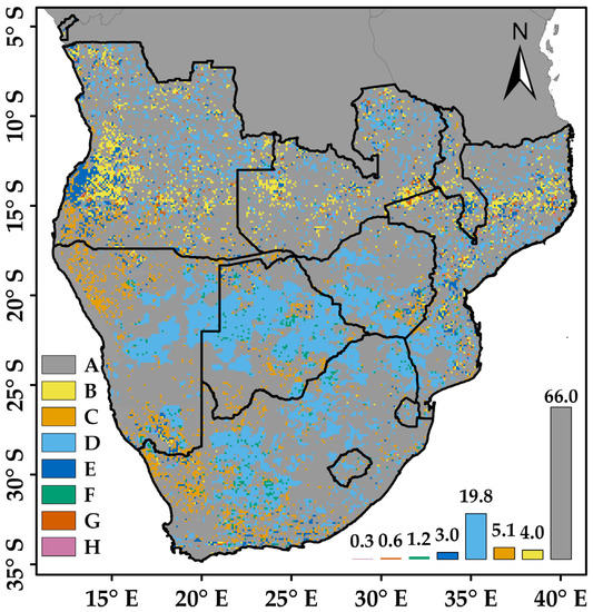
Figure 4.
Spatial distribution of combinations of different land degradation forms. Category A represents entirely undegraded land; categories B, C, and D represent visible, po-tential, and functional land degradation, respectively, without the other types of land degradation; category E, F, and G represent the co-occurrence of two types of land degradation as shown in Table 1; category H represents the co-occurrence of the three types of land degradation; the histogram in the figure indicates the proportions (%) of areas of different land degradation categories.
Detailed analysis of the three degradations and their relationship with precipitation trends was conducted (Figure 3 and Table 2). The major degradation categories (B, C, D, E) are presented in Table 2. In categories C and D, 11.76% (C7 + C8 + C9 + C10) of the potential land degradation and 56.88% (D5 + D6 + D7 + D8 + D11 + D12) of the functional land degradation areas exhibited a greening trend of the vegetation (visible land improvement) (Table 2). The proportions of precipitation in land degradation categories B, C, D, and E increased by 4.32%, 34.96%, 58.73%, and 10.1%, respectively (Table 2). A relatively low percentage of precipitation reduction occurred simultaneously with degradation, indicating that precipitation was not the main cause of land degradation (Table 2).
Table 2.
Proportions (%) of dynamics of annual rainfall, potential improvement, and functional improvement in degradation categories B, C, D, and E; the red and green arrows represent significant decrease and increase, respectively; the blank grid represents insignificant dynamics; the subcategories B, C, D, and E represent specific correspondence to the dynamics of indicators and rainfall.
3.2. Land Degradation across Land Covers and Countries
For areas with only one type of land degradation (situations B, C, D), category B (visible land degradation) had a higher proportion of area in forest (6.87%) and shrubland (3.37%) than other land covers (Table 3). Category C (potential land degradation) had a higher proportion in bare land (20.95%) and sparsely vegetated areas (16.67%) than other land covers; category D (functional land degradation) had a higher proportion in cropland (23.85), shrubland (22.95%), grassland (22.81%), sparse forest (16.55%), and vegetation (15.01%) than bare land (5.11%) (Table 3). Sparse vegetation and bare land exhibited greater proportions in category C than category D land degradation (Table 3).
Table 3.
The area proportions (%) of land degradation categories in each land cover. Category A represents entirely undegraded land; categories B, C, and D represent visible, potential, and functional land degradation, respectively, without the other types of land degradation; category E, F, and G represent the co-occurrence of two types of land degradation as shown in Table 1; category H represents the co-occurrence of the three types of land degradation.
We further determined the area (Figure S4) and its proportion (Figure 5 and Figure S5) of land degradation in each land cover for each country. Hotspots (regions with relatively large proportions of land degradation) of land degradation were identified by comparing the area proportion and the area of land degradation on the corresponding land cover in each country (Figure 5 and Figures S4 and S5). The hotspots of category B (visible degradation) included Angola’s forest, shrubland, and grassland; Mozambique’s shrubland; and Zambia’s shrubland (Figure 5a). The hotspots of category C (potential degradation) included Angola’s shrubland, grassland, bare land, and cropland; Zimbabwe’s forest; South Africa’s forest, grassland, and sparse vegetation areas; and Namibia’s shrubland and grassland (Figure 5b). The hotspots of category D (functional degradation) comprised Zimbabwe’s forest and shrubland; South Africa’s forest, grassland, sparse vegetation areas, and cropland; Botswana’s forest, shrubland, grassland, and cropland; and Namibia’s shrubland and bare land (Figure 5c). Category E (visible and potential land degradation) was mainly observed in Angola’s forest, shrubland, grassland, and cropland; Mozambique’s forest and shrubland; and Namibia’s sparse vegetation areas (Figure 5d). Category F (potential and functional land degradation) was mainly distributed in South Africa’s shrublands, grasslands, and sparsely vegetated areas; and Botswana’s shrublands. Category G (visible and functional land degradation) was mainly observed in the forests of Angola and Mozambique.
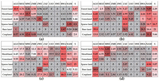
Figure 5.
The area proportion (%) of land degradation categories (a) B, (b) C, (c) D, and (d) E in each country and land cover. Darker colors show a higher proportion of land degradation; the gray shaded cells indicate correspondent pixels less than 50. S represents the mean level of the entire study area. It should be noted that the area proportion (%) of land degradation categories F, G, and H was minor and thus was shown in Figures S4 and S5 instead of the main text here.
4. Discussion
Spatial comparisons of degradation processes in previous studies (Table 4) indicated that different degradation assessments have corresponding degradation processes. Overlaying the analyses of degradation assessments provides information of land degradation. The findings in this study showed that the same degradation cause may result in multiple types of degradation, and the same indicator can correspond to more than one type of degradation.
Table 4.
Previous cases used to validate the results of this study.
4.1. The Land Degradation Processes behind the Different Measurement Methods
The results showed that 28.9% of the Southern Africa area was affected by one major type of land degradation, whereas 5.1% of the land surface was influenced by two or three types of land degradation. Three representative areas were selected and magnified to further clarify their relationships (Figure 6 and Figure 7). The first case was logging in south-western Angola (Figure 7a–d); the second was overgrazing and shrub encroachment in northern Namibia (Figure 7e–h); and the third was agricultural intensification (increased use of fertilizers and crop rotation) in cultivated cropland of South Africa (Figure 7i–l).
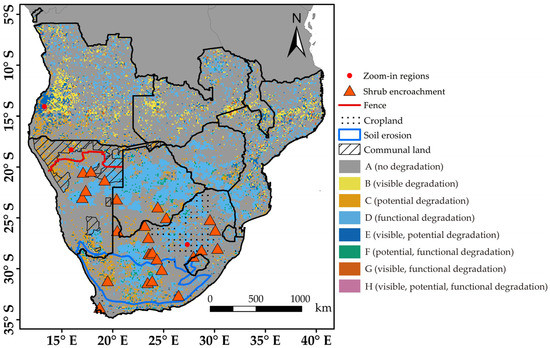
Figure 6.
The patterns of previous studies used for spatial comparison.
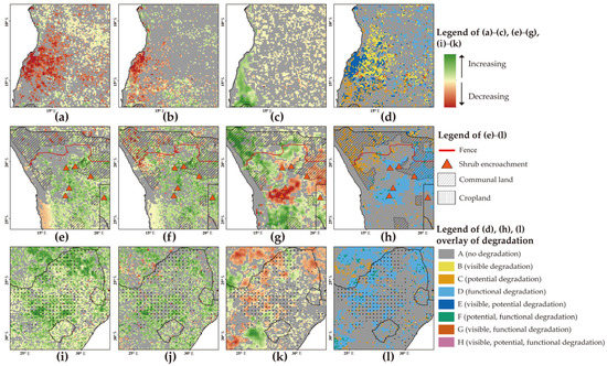
Figure 7.
The zoomed-in areas for the representative situations of land degradation: (a–d) indicate the multiple dynamics related to deforestation; (e–h) indicate the multiple dynamics related to shrub encroachment and overgrazing; (i–l) indicate the multiple dynamics related to agricultural intensification. Each row from left to right represents the visible land degradation, potential land degradation, functional land degradation, and the type of land degradation obtained by overlapping.
4.1.1. Potential and Visible Land Degradation Induced by Logging in Angola
Angola has large areas of category B, C, and E of degradation in south-western forestland, shrubland, and cropland (Figure 7a–d). Category B (co-occurrence of visible degradation and human-induced potential degradation) can be attributed to deforestation under agriculture extension [11]. The finding showed that the negative disturbance from human activities exceeded vegetation regeneration and then induced visible land degradation. Category C (functional degradation) indicates that human-induced potential land degradation was compensated by the regeneration of forests and increased rainfall (Table 2). This implies that although there was a risk of degradation, the vegetation can recover itself if human disturbance is maintained at a certain limit. Deforestation and cropland expansion significantly change the vegetation structure, and these areas exhibit an increase in SVR, since herbaceous plants and crops had higher SVR values than forests [22]. Category B (visible degradation) in the region demonstrated no potential land degradation and functional dynamics. This was because the severe destruction of vegetation alleviated the statistical relationship between vegetation and rainfall [20].
Deforestation and farmland expansion were also observed in other regions. In Zimbabwe, forests and grasslands were destroyed to make way for expansion of agricultural activities as part of the Fast Track land reform [52]. In Mozambique, forest degradation induced by timber harvesting and agriculture extension was observed on regional and local scales [11,53,54]. These processes were also observed in category E.
4.1.2. Functional and Potential Land Degradation Induced by Shrub Encroachment and Overgrazing in Northern Namibia
We digitized the spatial sites of shrub encroachment in Southern Africa (Figure 6) and focused on northern Namibia (Figure 7e–h). The spatial comparison showed that shrub encroachment was related to functional land degradation and visible and potential land improvement (Figure 7e–h), which is consistent with findings from previous research [21,22,30,49,55]. Shrub encroachment can be attributed to the occurrence of drought [30], and an increase in temperature [56]. This implies that the increase in vegetation greenness may be accompanied by degradation rather than what is indicated in the definition reported by UNCCD [1]. This result explains the recently observed inconsistent changes in vegetation greenness and productivity, which indicate a trade-off between structure and function in plant growth [57]. Shrub encroachment also has a significant impact on South Africa. The invasive woody plant of Prosopis species decreases the native grasses and herbaceous plants, which was reported in South Africa’s Nama Karoo and Savana [58]. The potential land degradation (category C) in northern Namibia’s grassland (Figure 7e–h) was mainly associated with overgrazing [13,50]. In this region, the land was communally owned, and thus overgrazing was prevalent (in extreme cases, livestock density exceeds the carrying capacity by over 40%) [13,59]. Furthermore, a vet fence was built to prevent disease spread, which limited the movement of livestock, thus exacerbating overgrazing [13,60]. Long-term overgrazing directly decreases the biomass of grasses and vegetation productivity, thus inducing land degradation.
4.1.3. Functional Land Degradation Induced by Agricultural Intensification in South Africa
Functional land degradation in South Africa is associated with agricultural intensification [51]. South Africa uses significantly higher volumes of fertilizers in agricultural production than other countries (Figure S6). The widespread use of fertilizers and irrigation strategies has led to an increase in food production in South Africa, despite a decrease in arable land [48]. Increased food production and positive agricultural management practices correspond to visible and potential land improvements in the region. Excessive use of fertilizers and irrigation can also cause salinization and soil erosion of cropland [51]. The integrated effect of over-reliance on agricultural management practices that reduce crop demand for precipitation and environmental deterioration leads to the reduced ability of crop to use precipitation. Severe functional land degradation types were observed in South Africa’s cropland (Figure 5 and Figure 7i–l). This demonstrated that well-intentioned human activities (agricultural management) can also induce a negative effect on the ecosystem. In western South Africa (Figure 6), soil erosion caused by overgrazing has further destroyed the soil structure, leading to the loss of nutrients required by plants and causing potential land degradation [14].
4.2. The Implication and Uncertainty
The data processing procedure and temporal scale of the three assessments were unified, such as calculating the optimal cumulative rainfall and vegetation relationships, using the maximum value of monthly NDVI to represent annual values, etc. These enabled the comparison of different types of land degradation, including visible, potential, and functional degradation. The hotspots of land degradation were identified in some countries, which can provide information for the formulation of national policies. Charcoal production is an important factor in growth of the national economy and infrastructure development, as well as a major source of income for local rural residents [12]. A high demand for timber harvesting associated with an increase in population causes land degradation [61]. A shift in the food supplement strategy in these countries changes the area for food production and harvesting, which directly promotes deforestation and forest degradation [48,62,63,64]. Therefore, the environmental impact should be considered when formulating policies for these countries with severe land degradation regions. The focus of this study was degradation, but sometimes degradation is associated with an increase in indicators, such as an increase in agricultural production with a decrease in SVR, and an increase in SVR with a decrease of forest cover in deforestation. Therefore, future studies should include information on these indicators to conduct land degradation analysis, thus improving the accuracy of the detection of degradation.
This study mainly focused on the analysis of the correspondence between degradation processes and indicators, but the impact of climate change was not fully explored. Climate change is a major cause of environmental change, and it also influences human behavior, so the study of land degradation processes should be conducted in the context of climate change in the future. Land cover change is also an important factor of land degradation, but it is difficult to quantify the land cover change from 1982 to 2015 due to the lack of continuous land cover datasets [65]. With the increasing accumulation of satellite observation data, future studies should improve the analysis of the impact of land cover change on land degradation.
5. Conclusions
Linear regression, TSS-RESTREND, and SeRGs methods were used in this study to explore three dimensions of vegetation degradation (visible, potential, and functional land degradation) in Southern Africa. The results indicated that the proportions of different land degradation types ranged between 8.0% and 21.9%, and the land improvement ranged between 22.2% and 46.2%. After overlapping different land degradation types, 28.9% of the study area (146.01 × 10⁴ km2) showed a single type of land degradation, whereas co-occurrence of land degradation was observed in 5.1% (25.95 × 10⁴ km2) of the study area. One indicator demonstrated degradation, whereas the other showed less degradation or no significant change. The use of a single indicator for land degradation evaluation results in an underestimation of the land degradation area. These findings indicate that these indicators were related to different aspects of the land degradation system after comparing them with the spatial patterns of land degradation reported in previous studies. Although vegetation greenness shows an increase, the risk of land degradation still exists. Therefore, the simultaneous use of multiple indicators is important for obtaining accurate results. The distribution of land degradation significantly varied across land covers and countries, which were attributed to various policies such as policies on agricultural intensification (cropland extension, overuse of fertilizers, etc.) and land use (overgrazing, vet fence, etc.). The overlapping of land degradation indicators provides a comprehensive view of land degradation in Southern Africa and improves our understanding of land degradation. These findings indicate the importance of using multiple indicators to understand land degradation.
Supplementary Materials
The following supporting information can be downloaded at: https://www.mdpi.com/article/10.3390/rs15020403/s1, Figure S1: (a) Pixels with a non-significant sensitivity of vegetation to rainfall (SVR) relationship in the TSS-RESTREND method; (b) the number of combinations of 15 years/3 pixels for the temporal and spatial windows that had a significant SVR on pixel scale; Figure S2: The percentage of significant rainfall–vegetation relationships in each combination of spatial and temporal windows; Figure S3: Area (100 km2) and its proportions of land degradation situations in different countries. SD: single and multiple land degradation; MD: multiple land degradation; Figure S4: The area (100 km2) of degradation situations (a) B, (b) C, (c) D, (d) E, (e) F, (f) G, (g) H in different countries and land covers; the gray shaded cell indicates the number of pixels of the correspondent type less than 50; Figure S5: The area proportion (%) of land degradation situations (a) F, (b) G, and (d) H in each country and land cover. Darker colors show a higher proportion of land degradation; the gray shaded cells indicate the number of pixels of the correspondent type lower than 50. S represents the mean level of the whole study area; Figure S6: (a) N, (b) P, and (c) K input per unit area of cropland. Data from FAO datasets.
Author Contributions
Conceptualization, Z.L., C.L., and S.W.; methodology, Z.L.; software, Z.L.; formal analysis, Z.L., C.L., S.W., and D.G.; writing—original draft preparation, Z.L.; writing—review and editing, C.L., S.W., and D.G.; visualization, Z.L.; supervision, C.L. and S.W.; funding acquisition, C.L. and S.W. All authors have read and agreed to the published version of the manuscript.
Funding
This research was jointly funded by the Strategic Priority Research Program of the Chinese Academy of Sciences (XDA19030201), the National Key Research and Development Program of China (No. 2017YFA0604701), and the Fundamental Research Funds for the Central Universities.
Data Availability Statement
Not applicable.
Conflicts of Interest
The authors declare no conflict of interest.
References
- UNCCD, Global Land Outlook: Secretariat of the United Nations Convention to Combat Desertification; UNCCD: Bonn, Germany, 2017; ISBN 9789295110489. Available online: https://www.unccd.int/resources/publications/global-land-outlook-1st-edition (accessed on 10 July 2020).
- Scholes, R.J.; Biggs, R. Ecosystem Services in Southern Africa: A Regional Assessment; CSIR: New Delhi, India, 2004; ISBN 0798855274. [Google Scholar]
- Maestre, F.T.; Eldridge, D.J.; Soliveres, S.; Kéfi, S.; Delgado-Baquerizo, M.; Bowker, M.A.; García-Palacios, P.; Gaitán, J.; Gallardo, A.; Lázaro, R.; et al. Structure and Functioning of Dryland Ecosystems in a Changing World. Annu. Rev. Ecol. Evol. Syst. 2016, 47, 215–237. [Google Scholar] [CrossRef] [PubMed]
- Prăvălie, R. Drylands Extent and Environmental Issues. A Global Approach. Earth Sci. Rev. 2016, 161, 259–278. [Google Scholar] [CrossRef]
- Wessels, K.J. Letter to the Editor: Comments on “Proxy Global Assessment of Land Degradation” by Bai et al. (2008). Soil Use Manag. 2009, 25, 91–92. [Google Scholar] [CrossRef]
- Gibbs, H.K.; Salmon, J.M. Mapping the World’s Degraded Lands. Appl. Geogr. 2015, 57, 12–21. [Google Scholar] [CrossRef]
- Angelo, M.J.; Du Plessis, A. Research Handbook on Climate Change and Agricultural Law; Edward Elgar Publishing: Cheltenham, UK, 2017; pp. 1–472. [Google Scholar] [CrossRef]
- Food and Agriculture Organization. Arid Zone Forestry: A Guide for Field Technicians; FAO Corporate Document Repository; FAO: Roma, Italy, 2016; pp. 1–12. [Google Scholar]
- Yao, J.; Liu, H.; Huang, J.; Gao, Z.; Wang, G.; Li, D.; Yu, H.; Chen, X. Accelerated Dryland Expansion Regulates Future Variability in Dryland Gross Primary Production. Nat. Commun. 2020, 11, 1–10. [Google Scholar] [CrossRef]
- Greve, P.; Orlowsky, B.; Mueller, B.; Sheffield, J.; Reichstein, M.; Seneviratne, S.I. Global Assessment of Trends in Wetting and Drying over Land. Nat. Geosci. 2014, 7, 716–721. [Google Scholar] [CrossRef]
- Curtis, P.G.; Slay, C.M.; Harris, N.L.; Tyukavina, A.; Hansen, M.C. Classifying Drivers of Global Forest Loss. Science (1979) 2018, 361, 1108–1111. [Google Scholar] [CrossRef] [PubMed]
- Zulu, L.C.; Richardson, R.B. Charcoal, Livelihoods, and Poverty Reduction: Evidence from Sub-Saharan Africa. Energy Sustain. Dev. 2013, 17, 127–137. [Google Scholar] [CrossRef]
- NAPCOD, Third National Action Programme for Namibia to Implement the United Nations Convention to Combat Desertification 2014–2024; Ministry of Environment and Tourism: Windhoek, Namibia, 2014. Available online: https://www.unccd.int/sites/default/files/naps/Namibia-2014-2024-eng.pdf (accessed on 10 July 2020).
- Bridges, E.M.; Oldeman, L.R. Global Assessment of Human-Induced Soil Degradation. Arid Soil Res. Rehabil. 1999, 13, 319–325. [Google Scholar] [CrossRef]
- Jiao, W.; Wang, L.; Smith, W.K.; Chang, Q.; Wang, H.; D’Odorico, P. Observed Increasing Water Constraint on Vegetation Growth over the Last Three Decades. Nat. Commun. 2021, 12, 3777. [Google Scholar] [CrossRef]
- Piao, S.; Wang, X.; Park, T.; Chen, C.; Lian, X.; He, Y.; Bjerke, J.W.; Chen, A.; Ciais, P.; Tømmervik, H.; et al. Characteristics, Drivers and Feedbacks of Global Greening. Nat. Rev. Earth Environ. 2020, 1, 14–27. [Google Scholar] [CrossRef]
- Li, C.; Fu, B.; Wang, S.; Stringer, L.C.; Wang, Y.; Li, Z.; Liu, Y.; Zhou, W. Drivers and Impacts of Changes in China’s Drylands. Nat. Rev. Earth Environ. 2021, 2, 858–873. [Google Scholar] [CrossRef]
- Baumgartner, P.; Cherlet, J. Institutional Framework of (in) Action against Land Degradation; Springer: Cham, Switzerland, 2015; ISBN 9783319191683. [Google Scholar]
- Wessels, K.J.; Prince, S.D.; Malherbe, J.; Small, J.; Frost, P.E.; VanZyl, D. Can Human-Induced Land Degradation Be Distinguished from the Effects of Rainfall Variability? A Case Study in South Africa. J. Arid Environ. 2007, 68, 271–297. [Google Scholar] [CrossRef]
- Burrell, A.L.; Evans, J.P.; de Kauwe, M.G. Anthropogenic Climate Change Has Driven over 5 Million Km2 of Drylands towards Desertification. Nat. Commun. 2020, 11, 1–11. [Google Scholar] [CrossRef]
- Verón, S.R.; Paruelo, J.M. Desertification Alters the Response of Vegetation to Changes in Precipitation. J. Appl. Ecol. 2010, 47, 1233–1241. [Google Scholar] [CrossRef]
- Abel, C.; Horion, S.; Tagesson, T.; De Keersmaecker, W.; Seddon, A.W.R.; Abdi, A.M.; Fensholt, R. The Human–Environment Nexus and Vegetation–Rainfall Sensitivity in Tropical Drylands. Nat. Sustain. 2021, 4, 25–32. [Google Scholar] [CrossRef]
- Burrell, A.L.; Evans, J.P.; Liu, Y. Detecting Dryland Degradation Using Time Series Segmentation and Residual Trend Analysis (TSS-RESTREND). Remote Sens. Environ. 2017, 197, 43–57. [Google Scholar] [CrossRef]
- Wessels, K.J.; van den Bergh, F.; Scholes, R.J. Limits to Detectability of Land Degradation by Trend Analysis of Vegetation Index Data. Remote Sens. Environ. 2012, 125, 10–22. [Google Scholar] [CrossRef]
- Wessels, K.J.; Prince, S.D.; Frost, P.E.; van Zyl, D. Assessing the Effects of Human-Induced Land Degradation in the Former Homelands of Northern South Africa with a 1 Km AVHRR NDVI Time-Series. Remote Sens. Environ. 2004, 91, 47–67. [Google Scholar] [CrossRef]
- Wingate, V.R.; Phinn, S.R.; Kuhn, N. Mapping Precipitation-Corrected NDVI Trends across Namibia. Sci. Total Environ. 2019, 684, 96–112. [Google Scholar] [CrossRef]
- Verón, S.R.; Oesterheld, M.; Paruelo, J.M. Production as a Function of Resource Availability: Slopes and Efficiencies Are Different. J. Veg. Sci. 2005, 16, 351–354. [Google Scholar] [CrossRef]
- Ratzmann, G.; Gangkofner, U.; Tietjen, B.; Fensholt, R. Dryland Vegetation Functional Response to Altered Rainfall Amounts and Variability Derived from Satellite Time Series Data. Biogeosciences Discuss. 2016, 8, 1–18. [Google Scholar] [CrossRef]
- Lian, X.; Piao, S.; Chen, A.; Huntingford, C.; Fu, B.; Li, L.Z.X.; Huang, J.; Sheffield, J.; Berg, A.M.; Keenan, T.F.; et al. Multifaceted Characteristics of Dryland Aridity Changes in a Warming World. Nat. Rev. Earth Environ. 2021, 2, 232–250. [Google Scholar] [CrossRef]
- Eldridge, D.J.; Bowker, M.A.; Maestre, F.T.; Roger, E.; Reynolds, J.F.; Whitford, W.G. Impacts of Shrub Encroachment on Ecosystem Structure and Functioning: Towards a Global Synthesis. Ecol. Lett. 2011, 14, 709–722. [Google Scholar] [CrossRef]
- Berdugo, M.; Delgado-Baquerizo, M.; Soliveres, S.; Hernández-Clemente, R.; Zhao, Y.; Gaitán, J.J.; Gross, N.; Saiz, H.; Maire, V.; Lehman, A.; et al. Global Ecosystem Thresholds Driven by Aridity. Science (1979) 2020, 367, 787–790. [Google Scholar] [CrossRef]
- Sedano, F.; Mizu-Siampale, A.; Duncanson, L.; Liang, M. Influence of Charcoal Production on Forest Degradation in Zambia: A Remote Sensing Perspective. Remote Sens. 2022, 14, 3352. [Google Scholar] [CrossRef]
- Mani, S.; Osborne, C.P.; Cleaver, F. Land Degradation in South Africa: Justice and Climate Change in Tension. People Nat. 2021, 3, 978–989. [Google Scholar] [CrossRef]
- Prăvălie, R. Exploring the Multiple Land Degradation Pathways across the Planet. Earth Sci. Rev. 2021, 220, 103689. [Google Scholar] [CrossRef]
- Smith, W.K.; Dannenberg, M.P.; Yan, D.; Herrmann, S.; Barnes, M.L.; Barron-Gafford, G.A.; Biederman, J.A.; Ferrenberg, S.; Fox, A.M.; Hudson, A.; et al. Remote Sensing of Dryland Ecosystem Structure and Function: Progress, Challenges, and Opportunities. Remote Sens. Environ. 2019, 233, 111401. [Google Scholar] [CrossRef]
- Rocha, J.C.; Peterson, G.; Bodin, Ö.; Levin, S. Cascading Regime Shifts within and across Scales. Science (1979) 2018, 362, 1379–1383. [Google Scholar] [CrossRef]
- GEIST, H.J.; LAMBIN, E.F. Dynamic Causal Patterns of Desertification. Bioscience 2004, 54, 817–829. [Google Scholar] [CrossRef]
- Campo-Bescós, M.A.; Muñoz-Carpena, R.; Southworth, J.; Zhu, L.; Waylen, P.R.; Bunting, E. Combined Spatial and Temporal Effects of Environmental Controls on Long-Term Monthly NDVI in the Southern Africa Savanna. Remote Sens. 2013, 5, 6513. [Google Scholar] [CrossRef]
- Mayaux, P.; Bartholomé, E.; Fritz, S.; Belward, A. A New Land-Cover Map of Africa for the Year 2000. J. Biogeogr. 2004, 31, 861–877. [Google Scholar] [CrossRef]
- Pinzon, J.E.; Tucker, C.J. A Non-Stationary 1981-2012 AVHRR NDVI3g Time Series. Remote Sens. 2014, 6, 6929–6960. [Google Scholar] [CrossRef]
- Beck, H.E.; Wood, E.F.; Pan, M.; Fisher, C.K.; Miralles, D.G.; van Dijk, A.I.J.M.; McVicar, T.R.; Adler, R.F. MSWep v2 Global 3-Hourly 0.1° Precipitation: Methodology and Quantitative Assessment. Bull. Am. Meteorol. Soc. 2019, 100, 473–500. [Google Scholar] [CrossRef]
- Burrell, A.L.; Evans, J.P.; Liu, Y. The Impact of Dataset Selection on Land Degradation Assessment. ISPRS J. Photogramm. Remote Sens. 2018, 146, 22–37. [Google Scholar] [CrossRef]
- Gessner, U.; Naeimi, V.; Klein, I.; Kuenzer, C.; Klein, D.; Dech, S. The Relationship between Precipitation Anomalies and Satellite-Derived Vegetation Activity in Central Asia. Glob. Planet Change 2013, 110, 74–87. [Google Scholar] [CrossRef]
- Adams, M. Lm . Br: An R Package for Broken Line Regression. Wp 2017. Available online: http://cran.itam.mx/ (accessed on 1 September 2019).
- Verbesselt, J.; Hyndman, R.; Newnham, G.; Culvenor, D. Detecting Trend and Seasonal Changes in Satellite Image Time Series. Remote Sens. Environ. 2010, 114, 106–115. [Google Scholar] [CrossRef]
- Chow, G.C. Tests of Equality Between Sets of Coefficients in Two Linear Regressions. Econometrica 1960, 28, 591. [Google Scholar] [CrossRef]
- Abel, C.; Horion, S.; Tagesson, T.; Brandt, M.; Fensholt, R. Towards Improved Remote Sensing Based Monitoring of Dryland Ecosystem Functioning Using Sequential Linear Regression Slopes (SeRGS). Remote Sens. Environ. 2019, 224, 317–332. [Google Scholar] [CrossRef]
- FAOSTAT. FAOSTAT: Statistical Database; FAO: Rome. Available online: https://www.fao.org/faostat/en/#data (accessed on 10 December 2020).
- Saha, M.V.; Scanlon, T.M.; Odorico, P.D. Examining the Linkage between Shrub Encroachment and Recent Greening in Water-Limited Southern Africa. Ecosphere 2015, 6, 1–16. [Google Scholar] [CrossRef]
- Klintenberg, P.; Seely, M. Land Degradation Monitoring in Namibia: A First Approximation. Environ. Monit. Assess. 2004, 99, 5–21. [Google Scholar] [CrossRef] [PubMed]
- Potter, P.; Ramankutty, N.; Bennett, E.M.; Donner, S.D. Characterizing the Spatial Patterns of Global Fertilizer Application and Manure Production. Earth Interact 2010, 14. [Google Scholar] [CrossRef]
- Bhatasara, S.; Helliker, K. The Party-State in the Land Occupations of Zimbabwe: The Case of Shamva District. J. Asian Afr. Stud. 2018, 53, 81–97. [Google Scholar] [CrossRef]
- Silva, J.A.; Sedano, F.; Flanagan, S.; Ombe, Z.A.; Machoco, R.; Meque, C.H.; Sitoe, A.; Ribeiro, N.; Anderson, K.; Baule, S.; et al. Charcoal-Related Forest Degradation Dynamics in Dry African Woodlands: Evidence from Mozambique. Appl. Geogr. 2019, 107, 72–81. [Google Scholar] [CrossRef]
- Sedano, F.; Silva, J.A.; Machoco, R.; Meque, C.H.; Sitoe, A.; Ribeiro, N.; Anderson, K.; Ombe, Z.A.; Baule, S.H.; Tucker, C.J. The Impact of Charcoal Production on Forest Degradation: A Case Study in Tete, Mozambique. Environ. Res. Lett. 2016, 11. [Google Scholar] [CrossRef]
- Venter, Z.S.; Cramer, M.D.; Hawkins, H.J. Drivers of Woody Plant Encroachment over Africa. Nat. Commun. 2018, 9, 1–7. [Google Scholar] [CrossRef]
- Zhao, M.; Running, S.W. Drought-Induced Reduction in Global Terrestrial Net Primary Production from 2000 through 2009. Science (1979) 2010, 329, 940–943. [Google Scholar] [CrossRef]
- Ding, Z.; Peng, J.; Qiu, S.; Zhao, Y. Nearly Half of Global Vegetated Area Experienced Inconsistent Vegetation Growth in Terms of Greenness, Cover, and Productivity. Earths Future 2020, 8, 10. [Google Scholar] [CrossRef]
- Shackleton, R.T.; le Maitre, D.C.; van Wilgen, B.W.; Richardson, D.M. The Impact of Invasive Alien Prosopis Species (Mesquite) on Native Plants in Different Environments in South Africa. S. Afr. J. Bot. 2015, 97, 25–31. [Google Scholar] [CrossRef]
- Coppock, D.L.; Crowley, L.; Durham, S.L.; Groves, D.; Jamison, J.C.; Karlan, D.; Norton, B.E.; Ramsey, R.D. Community-Based Rangeland Management in Namibia Improves Resource Governance but Not Environmental and Economic Outcomes. Commun. Earth Environ. 2022, 3, 32. [Google Scholar] [CrossRef]
- Mendelsohn, J.; Jarvis, A.; Roberts, C.; Robertson, T. The Atlas of Namibia: A Portrait of the Land and its People; David Philip: Cape Town, South Africa, 2003; Available online: https://www.researchgate.net/publication/263546846_Atlas_of_Namibia_A_Portrait_of_the_Land_and_its_People (accessed on 1 April 2021).
- Huber-Sannwald, E.; Palacios, M.R.; Moreno, J.T.A.; Braasch, M.; Peña, R.M.M.; de Verduzco, J.G.A.; Santos, K.M. Navigating Challenges and Opportunities of Land Degradation and Sustainable Livelihood Development in Dryland Social-Ecological Systems: A Case Study from Mexico. Philos. Trans. R. Soc. B Biol. Sci. 2012, 367, 3158–3177. [Google Scholar] [CrossRef] [PubMed]
- Heinen, S.; Esterhuizen, D. Zimbabwe Grain and Feed Annual Report; USDA Foreign Agricultural Service: Washington, DC, USA, 2017; pp. 1–8. Available online: https://apps.fas.usda.gov/newgainapi/api/report/downloadreportbyfilename?filename=GRAIN%20AND%20FEED%20ANNUAL%20REPORT%20_Pretoria_Zimbabwe_7-26-2017.pdf (accessed on 10 December 2022).
- Dube, E.; Tsilo, T.J.; Sosibo, N.Z.; Fanadzo, M. Irrigation Wheat Production Constraints and Opportunities in South Africa. S. Afr. J. Sci. 2020, 116, 1–6. [Google Scholar] [CrossRef]
- Shew, A.M.; Tack, J.B.; Nalley, L.L.; Chaminuka, P. Yield Reduction under Climate Warming Varies among Wheat Cultivars in South Africa. Nat. Commun. 2020, 11, 4408. [Google Scholar] [CrossRef]
- Zeng, Y.; Hao, D.; Huete, A.; Dechant, B.; Berry, J.; Chen, J.M.; Joiner, J.; Frankenberg, C.; Bond-Lamberty, B.; Ryu, Y.; et al. Optical Vegetation Indices for Monitoring Terrestrial Ecosystems Globally. Nat. Rev. Earth Environ. 2022, 3, 477–493. [Google Scholar] [CrossRef]


Disclaimer/Publisher’s Note: The statements, opinions and data contained in all publications are solely those of the individual author(s) and contributor(s) and not of MDPI and/or the editor(s). MDPI and/or the editor(s) disclaim responsibility for any injury to people or property resulting from any ideas, methods, instructions or products referred to in the content. |
© 2023 by the authors. Licensee MDPI, Basel, Switzerland. This article is an open access article distributed under the terms and conditions of the Creative Commons Attribution (CC BY) license (https://creativecommons.org/licenses/by/4.0/).