Examining Thresholding and Factors Impacting Snow Cover Detection Using Nighttime Images

Abstract

Nighttime remote sensing data from the Visible Infrared Imaging Radiometer suite day/night band (VIIRS DNB) enable snow cover detection from full moonlight reflection. Using nighttime data is particularly relevant in areas with limited daytime hours due to high latitudes. Previous studies demonstrated the potential of using thresholding methods in detecting snow, but more research studies are needed to understand the factors that influence their accuracy. This study explored seven thresholding algorithms in four case study areas with different characteristics and compared the classified snow results to the MODIS MOD10A1 snow cover product. The results found that Li thresholding delivers higher accuracies for most case studies, with an overall accuracy between 65% and 81%, while mean thresholding performed best in mountainous regions (70%) but struggled in other areas. Most false negatives are caused by forests, especially closed and evergreen forests. The analysis of NDVI data matches these findings, with the NDVI of false negatives being significantly higher than true positives. False positives appear to be primarily located in or around built-up areas. This study provides insights into where nighttime VIIRS DNB data can be used to increase snow cover data temporal and spatial coverage.

1. Introduction

Knowing which areas of the planet are covered by snow or ice is of major importance to many fields of earth sciences, including climatology, meteorology, and hydrology. Snow has an impact on both local environments and on global climate [1,2]. Since the beginning of remote sensing in the early 1970s, snow was one of the first to be investigated successfully because of its high albedo [3]. The introduction of MODIS (Moderate Resolution Imaging Spectroradiometer) enabled the creation of daily snow cover products at a global scale. Due to its high temporal resolution and global coverage, the MODIS snow cover product is widely used in many scientific fields, including climatology and hydrology [4]. The MODIS snow cover extent product continues to be actively released, and the most recent version of the product is version 6.1 of MOD10A1 [5], but the MODIS snow cover product is limited by light availability and cloud coverage. The limitation of low light is particularly impactful in high-latitude regions that receive few hours of daylight in winter months due to their position on the globe [6]. Even when there is sufficient light, the view of the ground may be limited by the presence of clouds. Beyond the limited winter availability of light, the impact of clouds is noticeable in both high-latitude regions and other potentially snow-covered areas in mid-latitude regions.

Satellite images captured during the night can circumvent both potential obstacles. The illumination from moonlight during certain lunar phases can be sufficient for detecting ground features with a high albedo, which also includes snow [7,8]. The ability to use illumination from moonlight means that data collection is not limited by the low number of daytime hours in winter in high-latitude regions.

The use of nighttime data would also increase the possibility of data being captured in cloud-free conditions anywhere on the planet. Regions covered by clouds during the day would have no data available. If clouds clear during the night, it is then possible to determine the snow cover extent. Combined with the assumption that there are fewer clouds at night due to the reduced convection, this means that more data would be available [9,10].

Snow detection with nighttime images has been around since the early days of nighttime satellites. The first attempts were made using the Defense Meteorological Satellite Program’s Operational Line-Scan System (DMSP-OLS) in the 1980s and 1990s, but their usefulness was limited due to their coarse resolution. Shortly after the launch of the Suomi National Polar Partnership (S-NPP) satellite equipped with VIIRS, the first study detecting snow cover was conducted, and it showed that this approach is feasible [6]. Further research into this field has come in recent years, with the two most notable studies being Huang et al. [7] and Liu et al. [11].

Miller et al. [6] was the first study to demonstrate that the detection of snow was possible using VIIRS DNB and its potential to provide additional data about snow coverage. While this study demonstrated the viability of the approach, it was based on visual identification, which limited its practical applications.

Later, Liu et al. [11] studied the classification of VIIRS DNB images using a Random Forest algorithm. They classified the image into four categories: snow, farmland, river, and other. The overall accuracy achieved in this study was 79.80%, and the kappa value was 0.45. They tested the approach to only one case study area, and it is still unknown how this approach performs in areas with different land-use and topographic characteristics. In addition, this approach is semi-automatic, requiring the operators to provide training and test labels, meaning that the results also depend on the quality of the manually created training and test data.

To the best of the authors’ knowledge, only one study has applied an automated algorithm to snow detection, and that is the minimum error thresholding algorithm by Huang et al. [7]. It demonstrated that automatic thresholding was possible for snow detection at night. They applied the minimum error thresholding algorithm to two case study areas. The overall accuracy reached 76.7% and 80.3% for each case study. The paper further analyzed the amount of data gaps that can be addressed using this approach and studied the impact of lunar phases on the results. However, it did not test the performance of different algorithms and only used two case study areas. While the variety of thresholding methods used for our specific purpose is limited, this is not the case in other areas of remote sensing. Moreover, for snow detection during the day, there have been studies that examined multiple different thresholding algorithms, including the study conducted by Yin et al. [12], which benchmarked nine different algorithms.

An additional challenge to nighttime snow detection ©s that other factors beyond snow cover can impact the brightness of the data collected and, therefore, the results. Huang et al. [7] looked at what an adequate lunar angle would be to determine snow cover extent and if there was a difference between different lunar phases. Land cover can also play a crucial role in VIIRS day/night band (DNB) data since different land covers have different albedos and, therefore, different pixel values when captured by the sensor. The impact of land cover on VIIRS data has already been documented in a study that showed that seasonal land cover change impacted the overall brightness of VIIRS DNB images [13].

Nighttime snow extent estimation is still in its early phases, and some questions still need to be answered before researchers can more widely adopt it. Two notable questions are as follows: (1) which thresholding methods perform best (under which conditions) and (2) what factors impact the accuracy of the methods.

This study examined seven automated thresholding algorithms to determine the best performance for snow detection using nighttime imagery captured by the S-NPP VIIRS DNB. After identifying the best automated threshold algorithm, the false estimates were analyzed to determine what factors influence the misclassifications. Improvements in this field can lead to a better understanding of what areas and under which conditions could be most suitable for snow cover detection at night. Furthermore, snow cover detection at night could further enable better spatial and temporal coverage of snow cover extent data, which could play a significant role in further understanding the impact snow coverage has on weather, climate, climate change, and hydrology.

2. Materials and Methods

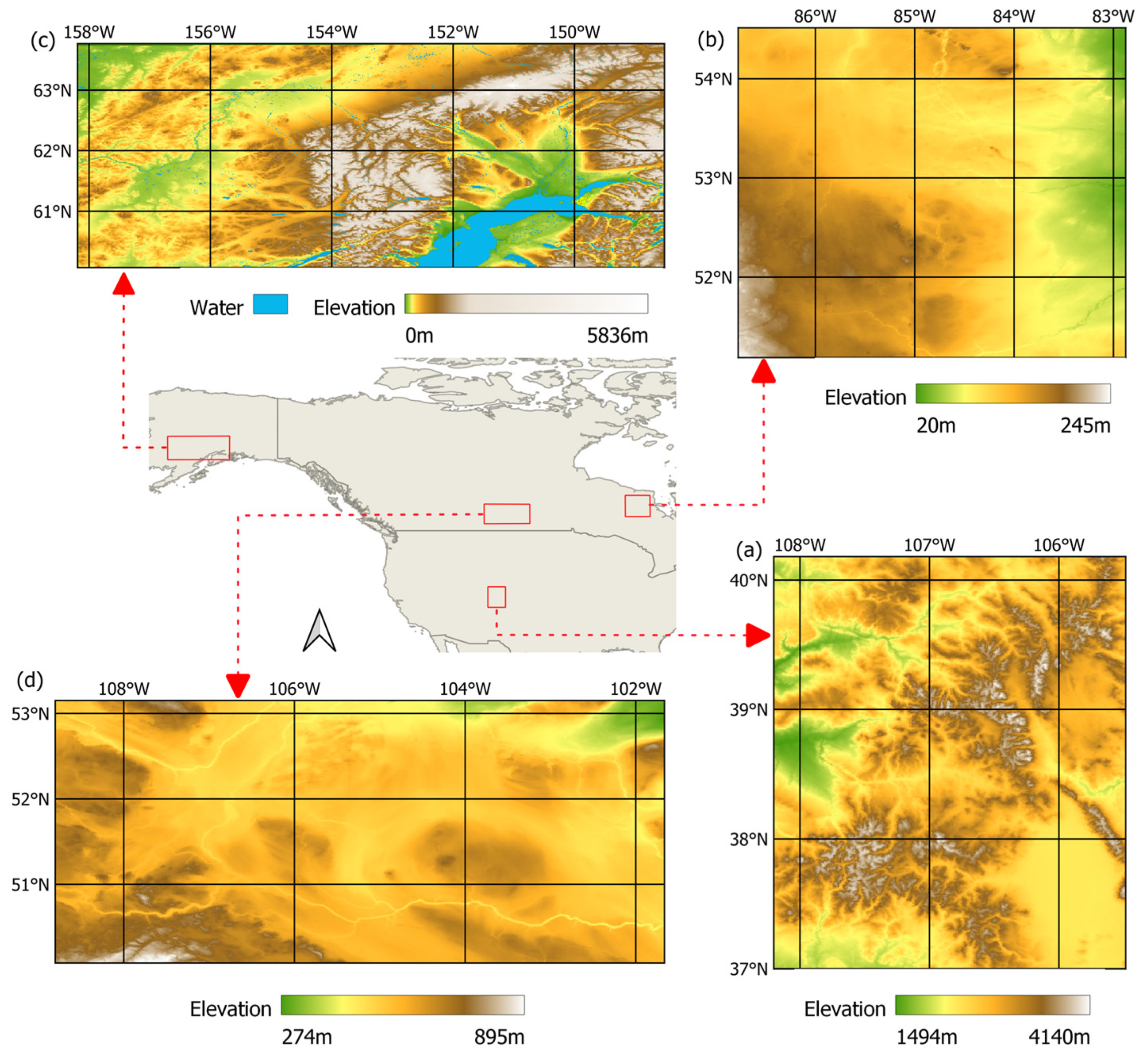
2.1. Case Study Areas

For the purposes of this study, four different case study areas were selected. The selection was made to incorporate different latitudes, elevations, topographies, and land covers. The four case study areas are spread throughout North America, including both the United States of America and Canada. The case study areas are located in Colorado, USA (a); Ontario, Canada (b); Alaska, USA (c); and Saskatchewan, Canada (d). Their extents are depicted in Figure 1.

The case study areas in Colorado (a) and Alaska (c) are primarily mountainous, with the area in Colorado encompassing a part of the Rocky Mountains, while on the other hand, the area in Alaska encompasses part of the Alaska Range. The major difference between the two areas lies in their latitude. The Colorado case study area is in a mid-latitude region, while the Alaska case study area is in a high-latitude region. Even though the Colorado case study area is not limited by the number of daytime hours due to it being located in a mid-latitude region, it can still experience cloud coverage during the day; therefore, it is included in this study as snow cover extent data can be added if nights are clear.

The other two case study areas are located in Canada and are mostly on flat terrain. The major difference between the two areas lies in their land cover, with the area in Saskatchewan (d) being primarily covered in cropland; in contrast, the area in Ontario (b) is covered mainly by several types of natural land cover, including several types of forests, shrubs, and herbaceous vegetation.

In addition to the geographic location of the case study areas, another important factor was selecting the exact date and time at which the data were captured. Three major factors determined the appropriate date for the data capture. The first factor was ensuring that the data were captured during a full moon. While Huang et al. [7] suggested that other lunar phases are also suitable for nighttime snow detection, only full moon phases were selected for this study to reduce the potential impact different lunar phases could have on the results. In addition to the data being captured during a full moon night, it was also essential to guarantee a sufficient number of day and night hours. Since this study uses both MODIS data captured during the day and VIIRS DNB data captured at night, only images from March and October were selected; during both of these months, there was snow cover in the selected case study areas, and both the day and night were sufficiently long for capturing data. Finally, the last factor was to ensure that there was no or little cloud coverage.

Table 1. Date and time of data collection by case study area.

Case Study	Location	VIIRS/MODIS Collection Date	VIIRS Time (Local)
a	Colorado	2 March 2018	01:30
b	Ontario	2 March 2018	03:24
c	Alaska	13 October 2019	05:06
d	Saskatchewan	21 March 2019	04:06

lists the exact dates of data collection for the four case study areas.

2.2. Data Collection

Data sources collected for the four case study areas included VIIRS DNB data for the nighttime snow extent estimates; the MODIS snow cover product for benchmarking; and land cover data to explore what factors could influence the false estimates.

Table 2. Study dataset names, spatial resolution, and links from which they can be accessed.

Dataset	Dates	Resolution
VIIRS DNB 1	2018–2019	750 m
MODIS Snow Cover 2	2018–2019	500 m
MODIS NDVI 3	2018–2019	500 m
Copernicus Land Use 4	2018–2019	10 m

¹ https://ladsweb.modaps.eosdis.nasa.gov/search/order/2/NPP_VDNES_L1--5000, (accessed on 6 May 2022). ² https://nsidc.org/data/mod10a1/versions/61 (accessed on 5 May 2022). ³ https://lpdaac.usgs.gov/products/mod09gav061/ (accessed on 7 May 2022). ⁴ https://land.copernicus.eu/global/products/lc (accessed on 7 May 2022).

lists the datasets used, including the acquisition date, spatial resolution, and access links.

The VIIRS DNB data were captured by the Suomi National Polar Partnership (S-NPP) satellite. The captured data were accessed at the Level-1 and Atmosphere Archive and Distribution System Distributed Active Archive Center (LAADS DAAC), operated by the National Aeronautics and Space Administration (NASA). The data were part of the NPP_VDNES_L1-VIIRS/NPP Day/Night Band 6-Min L1 Swath SDR 750 m product, and for this study, raw radiance values from the DNB were used [14].

MODIS snow cover extent data were also used in this study, specifically, the latest version 6.1 of the MOD10A1 snow cover extent product [5]. This data source was selected because it is commonly used in many hydrology and climate studies and has relatively high accuracy [4].

For land cover data, since this study covers different countries, it was important to select a land cover dataset with global coverage. Beyond global coverage, the level of detail with respect to the data was also an important factor in the selection, as a more detailed breakdown of forest and herbaceous vegetation types could lead to a clearer understanding of how different land covers impact snow detection. For this reason, Copernicus Global Land Service data were used for both 2018 and 2019 [15,16].

To calculate the NDVI, another MODIS product was used to guarantee consistency and data availability: version 6.1 of MOD09GA [17].

2.3. Data Preparation

To maximize the potential of accurate threshold calculations, parts of the VIIRS DNB data were masked as they were either not considered in this study, such as bodies of water, or because they emitted light, which could skew the data, such as built-up areas [7]. Copernicus land cover data were used to determine which parts of the VIIRS data should be masked. Areas masked out from the analysis included urban/built-up, permanent water bodies, and open sea. In this step, any clouds present would also have been masked, but since the case study areas were explicitly chosen to avoid cloud coverage, this step was not necessary for this study.

In order to ensure consistency between this study and previous studies, the same preparation steps outlined in Huang et al.’s studies [7,18] were used: MODIS snow cover extent data were processed to create a binary snow cover map. Pixels were marked as snow-covered, snow-free, or as no data (in case of cloud coverage or other data gaps). While VIIRS data were completely cloud-free, some cloud coverage was present in the MODIS data.

The NDVI values per case study area were calculated using the MOD09GA data source. The standard NDVI was used, where MOD09GA Band 1 is the red band and MOD09GA Band 2 is the near-infrared (NIR) band. The resulting NDVI maps for the case study areas ranged between −1 and 1, with values closer to 1 indicating higher vegetation presence.

As noted in Table 2, the four datasets used have different spatial resolutions. To address this, all datasets were resampled using the nearest neighbor operator to match VIIRS data.

2.4. Methodology

Seven different thresholding algorithms were selected and applied to the preprocessed VIIRS data. During the calculations, values that were previously masked during the preprocessing phase were not taken into consideration. The seven thresholding algorithms used are as follows: (1) Otsu [19], (2) Li [20], (3) Yen [21], (4) triangle [22], (5) minimum [23], (6) mean [23], and (7) Isodata [24]. While thresholding algorithms were initially created for different purposes, similarly to general computer vision, text identification, or microbiology, they have since been used in many fields, including remote sensing [25]. The seven algorithms are nonparametric and unsupervised. Their calculations are based on the histogram of all values present in the image. While the specific ways in which they are calculated vary from algorithm to algorithm, the end result of all algorithms is a numerical value that splits the results into two discrete categories. A succinct overview of the different algorithms was proposed by Sekertekin [25], where they also benchmarked the different methods, however, in the classification of water.

Following this step, the binary snow cover maps made by thresholding (test datasets) were compared to MODIS binary snow cover data for the same case study area (reference dataset). All pixels where there were data available in both the test and the reference dataset were considered true positive (TP), true negative (TN), false positive (FP), or false negative (FN).

There are two distinct ways in which these results can be displayed, which serve different purposes. The first is to create a confusion matrix (calculating the percentage value for each category in the entire case study area). The confusion matrix is particularly useful in order to determine the overall accuracy of the thresholding results in comparison to the MODIS snow cover product. Specifically, the higher the sum of the true positive and true negative percentages, the more accurate the thresholding snow cover extent. The second way is to map the accuracy results. This is particularly important to determine which factors cause both false negatives and false positives. By mapping their position, it is possible to relate the performance per land cover category and relate it to the NDVI value.

Discriminating the results into discrete categories enables determining if any particular characteristic impacts the overall accuracy. This entails the creation of confusion matrices per land cover category as previously proposed in a study by Yang et al. [26]. If the land cover has no or a limited impact on the results, the accuracy should be relatively consistent between different land covers. Conversely, if specific land covers do impact the results, the accuracy within those should vary significantly.

Furthermore, version five of the MODIS snow cover product treated areas with high NDVI values separately from regions with low NDVI values [27]; therefore, this study also investigated the influence of NDVI. In version five of the MODIS snow cover product, areas with high NDVI values were given a lower threshold in order to be considered snow-covered compared to areas with low NDVI values [27]. If the impact of NDVI on VIIRS matches the impact it had on MOIDS, it is expected that the NDVI values of pixels marked as false negatives would be higher than those marked as true positives, indicating that the potential reason for the misclassification would be the NDVI. This factor was examined by looking at the distribution and mean values of the NDVI of true positives and false negatives per case study area.

Finally, some false positive and false negative values might not be explainable using the methods outlined above; therefore, visual analysis was also performed to explore possible hypotheses explaining some of the results and potentially create the basis for further research.

3. Results

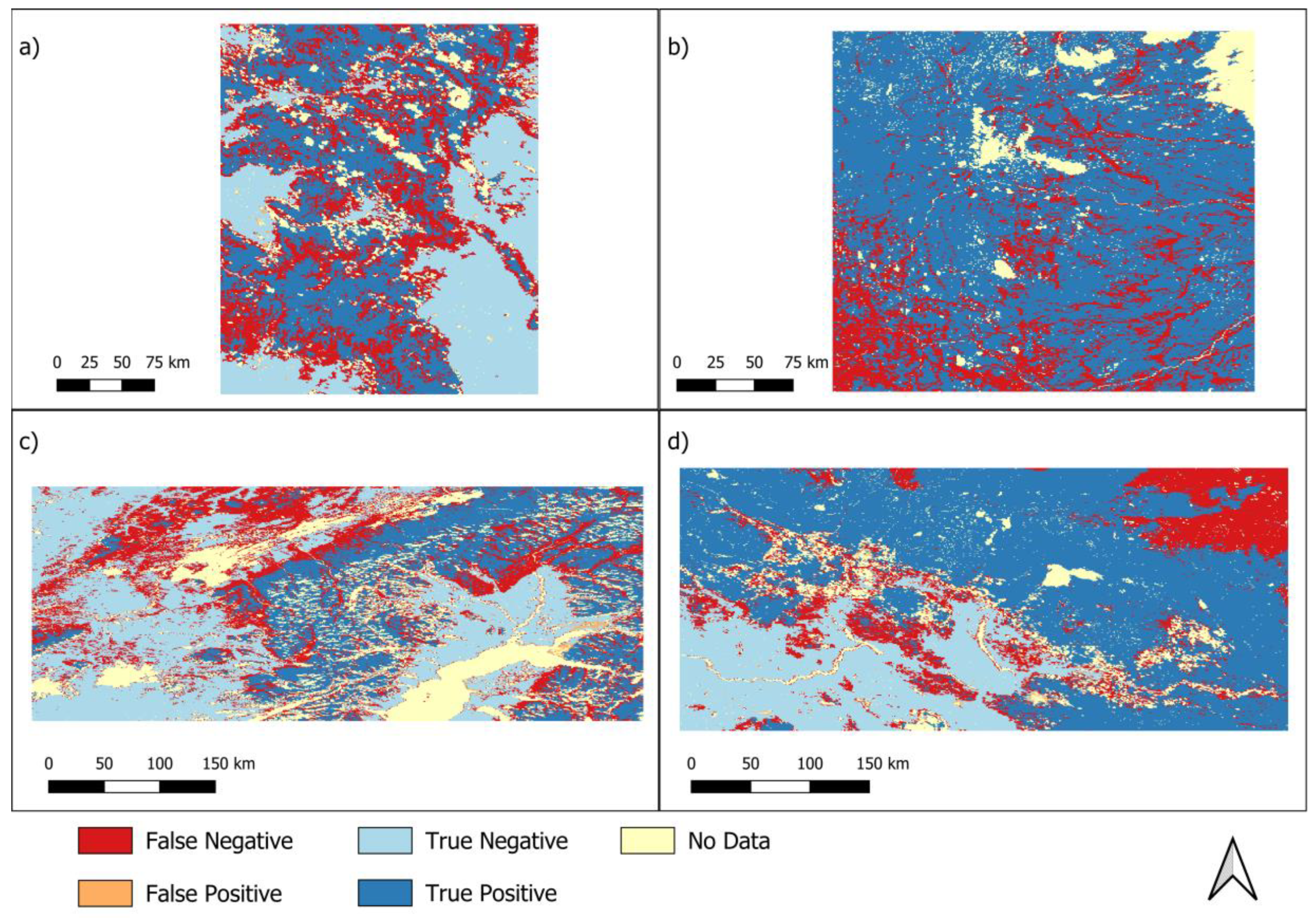
3.1. Overall Thresholding Results

The confusion matrices of the seven different thresholding algorithms for the four case study areas are shown in

Table 3. Confusion matrix, overall accuracy, errors, and Cohen’s kappa for the seven thresholding algorithms and the four case study areas.

Case Study	Thresholding Algorithm	TP	TN	FP	FN	Overall Accuracy	Kappa
a. Colorado	Otsu	28.42	31.32	0.14	40.13	59.73	0.31
	Li	36.86	31.19	0.26	31.68	68.05	0.42
	Yen	0.03	31.44	0.01	68.51	31.47	0.00
	Triangle	7.98	31.42	0.04	60.57	39.40	0.08
	Minimum	0.01	31.45	0.00	68.54	31.45	0.00
	Mean	38.36	31.15	0.30	30.19	69.51	0.44
	Isodata	29.73	31.30	0.16	38.82	61.02	0.32
b. Ontario	Otsu	62.34	0.00	0.00	37.66	62.34	n/a
	Li	69.17	0.00	0.00	30.83	69.17	n/a
	Yen	77.91	0.00	0.00	22.09	77.91	n/a
	Triangle	0.07	0.00	0.00	99.93	0.07	n/a
	Minimum	0.00	0.00	0.00	100.00	0.00	n/a
	Mean	54.75	0.00	0.00	45.25	54.75	n/a
	Isodata	64.97	0.00	0.00	35.03	64.94	n/a
c. Alaska	Otsu	19.17	40.25	0.22	40.36	59.42	0.27
	Li	25.72	40.16	0.31	33.81	65.88	0.37
	Yen	0.01	40.42	0.05	59.53	40.42	0.00
	Triangle	0.20	40.39	0.08	59.33	40.59	0.00
	Minimum	0.00	40.47	0.00	59.53	40.47	0.00
	Mean	30.50	40.03	0.44	29.03	70.53	0.45
	Isodata	23.38	40.19	0.27	36.15	63.57	0.34
d. Saskatchewan	Otsu	55.10	22.26	0.17	22.47	77.36	0.52
	Li	59.37	22.21	0.22	18.20	81.58	0.59
	Yen	0.02	22.38	0.04	77.55	22.41	0.00
	Triangle	0.15	22.34	0.08	77.42	22.50	0.00
	Minimum	0.00	22.42	0.00	77.57	22.42	0.00
	Mean	52.68	22.27	0.16	24.89	74.95	0.48
	Isodata	55.10	22.26	0.17	22.47	77.36	0.52

. The results are expressed as percentages, with the number representing the total fraction of the classification relative to the total number of all classified pixels. Both the overall accuracy (the sum of both the true positive and true negative percentages) and Cohen’s kappa [28,29] are included in Table 3.

In Figure 2, the thresholding method with the best overall accuracy was used to map the confusion matrix. For the Colorado and Alaska case study areas, mean thresholding was used; for the Ontario case study area, Yen thresholding was used; finally, Li thresholding results were used for the Saskatchewan case study area. The resulting four maps for the case study area show the geographic locations of TP, TN, FP and FN values.

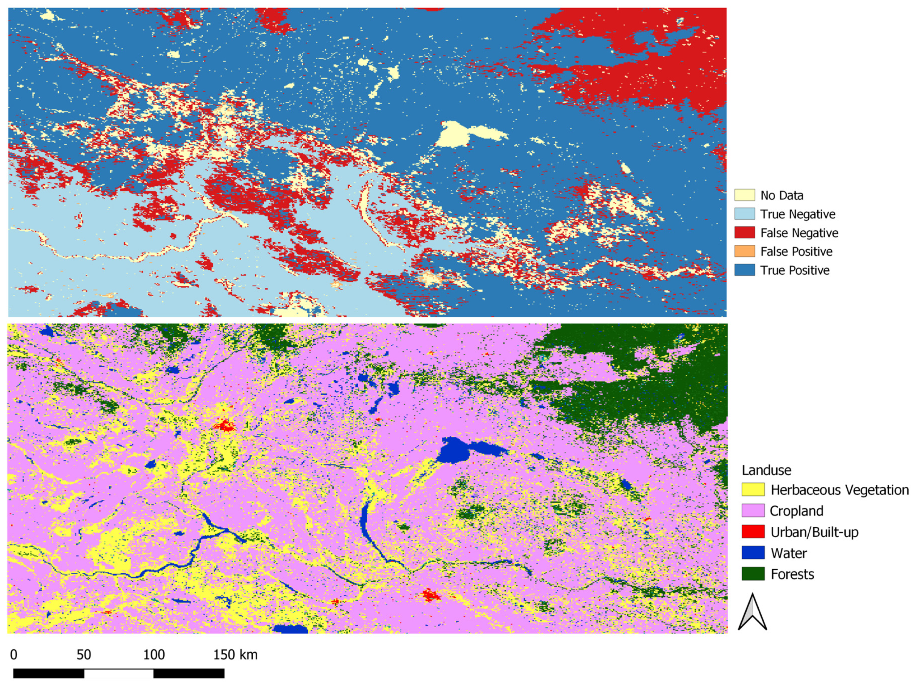
3.2. Land Cover Discrimination

The mapping of the confusion matrix values onto their geographic location also enabled the creation of discrete results per land cover type. For this, the maps from Figure 2 were compared per land cover type of the Copernicus data for the appropriate year [15,16]. The resulting confusion matrices (

Table 4. Confusion matrix per land cover type for the four case study areas.

Case Study	Thresholding Algorithm	TP	TN	FP	FN	Overall Accuracy	Kappa
a. Colorado	Shrubs	25.45	58.43	0.73	15.39	83.88	0.65
	Herbaceous vegetation	46.45	41.22	0.46	11.88	87.67	0.76
	Cultivated and managed vegetation/agriculture	7.72	86.68	0.64	4.95	94.40	0.70
	Bare/sparse vegetation	73.37	24.09	0.13	2.37	97.50	0.93
	Closed forest, evergreen needle leaf	22.81	15.33	0.08	61.77	38.15	0.10
	Closed forest, deciduous broad leaf	70.13	0.11	0.03	29.74	70.24	0.00
	Closed forest, unknown	43.42	20.74	0.14	35.69	64.16	0.33
	Open forest, evergreen needle leaf	34.72	21.94	0.18	43.15	56.66	0.26
	Open forest, deciduous broad leaf	72.95	0.07	0.00	26.99	73.01	0.00
	Open forest, unknown	43.14	29.40	0.24	27.22	75.86	0.54
b. Ontario	Shrubs	85.81	0.00	0.00	14.19	85.81	n/a
	Herbaceous vegetation	94.17	0.00	0.00	5.83	94.17	n/a
	Herbaceous wetland	97.09	0.00	0.00	2.91	97.09	n/a
	Closed forest, evergreen needle leaf	36.94	0.00	0.00	63.06	36.94	n/a
	Open forest, evergreen needle leaf	63.92	0.00	0.00	36.08	63.92	n/a
	Open forest, unknown	74.73	0.00	0.00	25.27	74.73	n/a
c. Alaska	Shrubs	20.65	56.49	0.25	22.61	77.14	0.50
	Herbaceous vegetation	48.50	33.71	0.31	17.48	82.21	0.65
	Bare/sparse vegetation	84.51	1.14	0.28	14.06	85.66	0.12
	Snow and Ice	78.48	0.18	0.03	21.30	78.67	0.01
	Herbaceous wetland	3.37	82.83	2.28	11.52	86.20	0.27
	Closed forest, evergreen needle leaf	6.13	38.31	0.35	55.22	44.44	0.07
	Closed forest, mixed	0.95	69.95	2.47	26.63	70.90	0.00
	Closed forest, unknown	6.66	56.01	0.74	36.59	62.67	0.16
	Open forest, evergreen needle leaf	11.60	31.55	0.91	55.93	43.16	0.10
	Open forest, unknown	12.24	58.13	0.45	29.18	70.37	0.32
d. Saskatchewan	Herbaceous vegetation	48.16	37.93	0.59	13.33	86.08	0.72
	Cultivated and managed vegetation/agriculture	67.79	20.76	0.13	11.31	88.55	0.71
	Herbaceous wetland	62.41	20.66	0.18	16.75	83.07	0.60
	Closed forest, evergreen needle leaf	6.43	0.08	0.00	93.50	6.50	0.00
	Closed forest, deciduous broad leaf	29.14	0.22	0.00	70.63	29.37	0.00
	Closed forest, mixed	3.46	0.07	0.00	96.48	3.52	0.00
	Closed forest, unknown	35.92	5.77	0.00	58.31	41.69	0.07
	Open forest, evergreen needle leaf	57.12	0.92	0.00	41.96	58.04	0.02
	Open forest, deciduous broad leaf	58.94	0.26	0.00	40.80	59.20	0.01
	Open forest, unknown	60.25	7.63	0.08	32.03	67.88	0.22

) discriminate the per land cover type. As the four case study areas cover different geographic regions, there are differences between the land cover types present in them. Additionally, some land cover types are infrequent in some case study areas; therefore, land covers with under 500 appearances were removed from the results.

3.3. NDVI Influence

NDVI values were also investigated in this study. If false negative areas have a higher NDVI than true positives, this may indicate that the thresholding value should be lower for the areas with higher NDVI. In order to determine if the NDVI values are higher, two boxplots per case study area were created: one for true positives and one for false negatives. The boxplots indicate mean values, the first and third quantiles of the data, and the minimum and maximum (see Figure 3).

3.4. Additional Factors

To explain false positives (which account for less than 1% of the pixels), visual analyses were performed. What is clearly noticeable in the spatial distribution of false positives is the proximity to urban/built-up areas. Examples of this phenomenon can be observed in Figure 4, where the built-up areas from the Copernicus data are presented, as well as false positives. The Ontario case study area had no false positives; therefore, it was not included in the visual analysis.

Even though most false negatives occurred in forested areas, other land covers also had false negatives. The distribution and cause of these cannot be explained by tree canopies; therefore, another factor must be their cause. The two different false negatives can be best observed in the Saskatchewan case study area, which is pictured in Figure 5. While the false negative values in the north and northeast can be explained by the forest present there, the false negatives in the center and southwest are present in a mixture between cropland and herbaceous vegetation.

4. Discussion

The seven thresholding algorithms investigated in this study had notably different performances. The overall accuracy varied for each algorithm and between the four case study areas, but some overall conclusions can still be drawn from them. The overall accuracy of the algorithms had quite widespread values, with the lowest overall accuracy being 0%, while the highest overall accuracy was 81.58%.

The two thresholding algorithms that performed the worst were triangle thresholding and minimum thresholding, both of which had their highest overall score at only around 40%. Similarly, Yen thresholding also had results of less than or approximately 40%, with the exception of the Ontario case study area, where it performed the best with a 77.91% overall accuracy. Otsu and Isodata thresholding had middling performances in all four case study areas, with neither of them being the best-performing one in any case study area. Their overall accuracies ranged between 59% and 77%. Another algorithm, mean thresholding, had a similar range of overall accuracy, with its lowest result being 54.75% and the highest being 74.95%. However, what is notable is that mean thresholding was the best-performing algorithm in both the Colorado and Alaska case study areas. However, it underperformed in the Ontario case study area, where it achieved only a 54.75% overall accuracy. These results indicate that mean thresholding is the best-performing algorithm in mountainous regions, as both the Colorado and Alaska case study areas are predominantly mountainous.

While mean thresholding performed the best in mountainous areas, the algorithm with the best range of overall accuracy and the highest individual accuracy in the Saskatchewan case study area was Li thresholding. This algorithm always had an overall accuracy above 65% and was either the highest or second-highest result in every case study area. Therefore, even though mean thresholding did have the best result in two out of the four case study areas, the results indicate that its choice depends on context. The fact that mean thresholding measurably underperformed in the Ontario case study area means that in order to ensure the best overall and consistently high overall accuracy, the Li thresholding algorithm is the best choice out of all seven algorithms tested in this study. If the thresholding is applied exclusively to mountainous areas, using mean thresholding could yield better results. However, if various terrains are present, Li thresholding will provide fair overall and consistent results.

The highest overall accuracy results among all case studies range between 70% and 82%, which is comparable with the results achieved by Huang et al. [7], where the overall accuracy reached 77% and 80%. Moreover, similarly to the results achieved by Liu et al. [11], the overall accuracy reported was 80% and the Kappa coefficient was 0.45. Therefore, the results were also within the range of the maximums achieved by the thresholding algorithms in this study.

Determining the best thresholding algorithm is not the only conclusion that can be drawn from the results. What is especially noteworthy is the difference between false positives and false negatives. The percentage of false negatives is significantly larger than the false positives for all thresholding algorithms and in all case study areas. In fact, false positives in every case study area and thresholding algorithm make up less than 0.5%. This indicates that the vast majority of overall error comes from the underestimation of the snow extent by the VIIRS DNB snow extent model when compared to the MODIS snow cover product.

The causes of this underestimation and the locations where it occurs can be potentially explained by the land cover’s presence. While the four case study areas had different land cover types present, some overall trends are still noticeable. The two land covers that had the lowest overall accuracy in all case study areas are open and closed evergreen needle leaf forests. Besides those two, all other types of forests, when present in the case study area, had lower overall accuracies than non-forest land covers such as shrubs or herbaceous vegetation. Considering forest types, evergreen needle leaves had the lowest overall accuracy, but when comparing open and closed forests, closed forests have lower overall accuracies. In all cases, the low overall accuracy can be entirely explained by false negatives, with false positives being rare or nonexistent for most forests. The remaining non-forested areas performed well with high true-positive and true-negative values, resulting in high overall accuracy. The false negatives were in the 10–25% range, and false positives were present but usually made up less than 1%.

The effect that forests have on the accuracy of snow cover extent is not unexpected. Forests have been a factor that limited the accuracy of snow cover extent estimates in many different products. The presence of tree canopies would effectively block the view of the ground and, therefore, any snow that is present, causing underestimations [30]. Furthermore, while it is possible that the canopy itself would capture some of the snow and therefore increase its albedo, studies suggest that even when that does occur, the overall albedo is still lower [31].

The differences between closed and open forests relate mainly to their canopies. In the Copernicus land cover data, closed forests were considered all areas that have more than 70% of the ground covered by canopies, while open forests have 15–70% canopy cover [32]. Since canopies cover more of the view of the ground and any snow present there in closed forests, they would have more false negative estimates than in open forests, where more of the ground is visible.

The impact of canopies would also explain the lower overall accuracy of evergreen forests compared to other forest types. In most cases, the evergreen forests performed roughly 20–30% worse than other types of forests. This relates to the fact that the images were captured during March and October, when evergreen trees still retain their full canopy while deciduous trees have lost most of their canopy. The lack of canopies in deciduous forests would mean that the ground—and therefore any potential snow on the ground—would be more visible and therefore easier to classify.

Another way in which this effect could possibly be measured is by investigating the NDVI. As tree canopies, and especially evergreen trees, should have a high NDVI value at the time the data were captured, it would be expected that the NDVI values of the false negatives would show consistently higher values than the NDVI in true positives. As observed from the box plots in Figure 3, the mean, quantiles, and maximum values of the NDVI are higher for false negatives than for true positives. This indicates that a higher NDVI is correlated with false-negative identification. This factor, combined with the previous discussion of the impact of forest canopies, suggests that high-density forests and especially evergreen forests have the most negative impact on identification.

The cause of the false negatives can be explained by their location at the periphery of the snow cover. Because these areas mark the transition between snow and no snow, they should have relatively shallow snow depth. Studies have shown that even during the day, the accuracy of remote sensing of snow decreases with lower snow depths [26]. Therefore, nighttime snow detection accuracy seems to also be susceptible to underestimations with low snow depth, explaining the underestimates in those periphery regions. The snow depth could have also slightly changed in the period between when MODIS and VIIRS DNB data were captured, which could explain some of the discrepancies between them. While in most non-forested areas, the VIIRS DNB data performed well, the accuracy of the boundaries will only become apparent with an in situ study, which could analyze the impact of snow depth on the accuracy.

The spatial distribution of false positives (e.g., in Figure 4) clearly shows that most false negatives are within the vicinity of urban/built-up areas. This is predominant near the larger built-up areas present in case study areas such as Anchorage in Alaska or Saskatoon and Regina in Saskatchewan. While the specific built-up areas were masked during the data preparation step, the surrounding areas were noticeably much brighter due to human activity. Our quantitative analysis of the accuracy within the different land covers is affected by the accuracy of the land cover reference dataset. If urban areas are underestimated in the reference dataset, we overestimate the false positives as not enough build-up is masked.

This phenomenon has been described in previous studies suggesting that suburban and rural areas do emit more artificial light toward the horizon, making the surrounding area brighter [33]. However, not all false positives are obviously near built-up areas (or at least near areas categorized as urban/built-up land cover). When exploring FPs distant from built-up land cover, we observed that a majority of these false positives still appear to be linked to human activity, but it is not enough to mark the area as built-up in the land cover dataset. This is true in the case of smaller communities, such as the town of Beechy in Saskatchewan, which is categorized as cropland due to its small size and population (the predominant land cover that completely surrounds the town). While being relatively small, there is still enough artificial light emitted to skew the results into false positives. Other areas in the three case study areas with false positive results follow the same pattern. While this approach seems to explain the false positives, it remains only a visual identification of the pattern, and to determine if it is the main reason behind it, a more rigorous and analytical study would be necessary. One way to (potentially) avoid these false positives is by creating a mask layer that is not based on land use but instead on light. Since the NASA Black Marble product suite releases monthly and annual data, it could be used to create a mask layer as all the brightest areas would be a result of human activity [34]. This approach would also remove uncertainty caused by inaccuracies of the land cover data.

Naturally, this study has certain limitations that can have some impact on the results. The main limitation is that the VIIRS snow cover extent is compared to another snow cover model and not to in situ measurements. The selected MODIS snow cover product has known limitations [35], but it is still a widely used model, and agreement between the models still indicates that it is acceptable for many studies in hydrology, climate science, or other areas where MODIS data are commonly used [4].

Exploring accuracies in evergreen or all forested areas is an avenue for further research. Daytime snow cover extent products have dealt with the forest issues [30], and improving the results in those areas could be possible by following the strategy of lowering the threshold for areas with high NDVI or by calculating a separate threshold for forested areas.

Furthermore, since future Joint Polar Satellite System (JPSS) missions are already planned and will be equipped with VIIRS, data availability in the future will only increase [36]. Hopefully, this will reduce the impact cloud coverage has on VIIRS DNB data as multiple satellites will be capturing the data, enabling even better coverage in the future.

Identifying snow cover extent using VIIRS DNB data is possible and achievable with relatively high overall accuracy. The false estimates are usually underestimations, with overestimations present but usually limited to areas near human activity. The false negatives are usually present in forested areas, especially in closed and evergreen forests. Some false negatives also occur on the border between areas covered and not covered by snow. While this could impact the usefulness of the VIIRS DNB data for some purposes, this is an area where the results could be improved with in situ research.

5. Conclusions

Of the seven tested thresholding algorithms, Li thresholding achieved the most consistently high overall accuracy in all case study areas, while the mean thresholding algorithm performed the best in mountainous regions, but it did not have high overall accuracies in other areas. Depending on the use case, either of the two thresholding algorithms could provide results that would be useful for climate or hydrology research. If the terrain of the case study area is diverse or if there are multiple different areas, Li thresholding seems to be the most effective option. If the case study is predominantly mountainous, then mean thresholding can potentially achieve better results. While some limitations are present, the high overall accuracy and the distribution of accurate identification should still prove useful in filling in some spatial or temporal data gaps for snow cover extent maps, especially in regions with few forests.

References

1. Levis, S.; Bonan, G.B.; Lawrence, P.J. Present-Day Springtime High-Latitude Surface Albedo as a Predictor of Simulated Climate Sensitivity. Geophys. Res. Lett. 2007, 34, 1–4. [Google Scholar] [CrossRef]
2. Musselman, K.N.; Clark, M.P.; Liu, C.; Ikeda, K.; Rasmussen, R. Slower Snowmelt in a Warmer World. Nat. Clim. Chang. 2017, 7, 214–219. [Google Scholar] [CrossRef]
3. Foster, J.L.; Hall, D.K. Observations of Snow and Ice Features during the Polar Winter Using Moonlight as a Source of Illumination. Remote Sens. Environ. 1991, 37, 77–88. [Google Scholar] [CrossRef]
4. Da Ronco, P.; Avanzi, F.; De Michele, C.; Notarnicola, C.; Schaefli, B. Comparing MODIS Snow Products Collection 5 with Collection 6 over Italian Central Apennines. Int. J. Remote Sens. 2020, 41, 4174–4205. [Google Scholar] [CrossRef]
5. Hall, D.K.; Riggs, G.A. MODIS/Aqua Snow Cover Daily L3 Global 500 m Grid, Version 61; NASA National Snow and Ice Data Center Distributed Active Archive Center: Boulder, CO, USA. [CrossRef]
6. Miller, S.D.; Straka, W.; Mills, S.P.; Elvidge, C.D.; Lee, T.F.; Solbrig, J.; Walther, A.; Heidinger, A.K.; Weiss, S.C. Illuminating the Capabilities of the Suomi National Polar-Orbiting Partnership (NPP) Visible Infrared Imaging Radiometer Suite (VIIRS) Day/Night Band. Remote Sens. 2013, 5, 6717–6766. [Google Scholar] [CrossRef]
7. Huang, Y.; Song, Z.; Yang, H.; Yu, B.; Liu, H.; Che, T.; Chen, J.; Wu, J.; Shu, S.; Peng, X.; et al. Snow Cover Detection in Mid-Latitude Mountainous and Polar Regions Using Nighttime Light Data. Remote Sens. Environ. 2022, 268, 112766. [Google Scholar] [CrossRef]
8. Lee, T.E.; Miller, S.D.; Turk, F.J.; Schueler, C.; Julian, R.; Deyo, S.; Dills, P.; Wang, S. The NPOESS VIIRS Day/Night Visible Sensor. Bull. Am. Meteorol. Soc. 2006, 87, 191–200. [Google Scholar] [CrossRef]
9. Foster, J.L. Observations of the Earth Using Nighttime Visible Imagery; Aitken, G.W., Ed.; SPIE: Arlington, MA, USA, 1983; pp. 187–193. [Google Scholar]
10. Wiesnet, D.R.; Mcginnis, J.; Matson, M.; Pritchard, J.A. Evaluation of Hcmm Satellite Data for Estuarine Tidal Circulation Patterns and Thermal Inertia Soil Moisture Measurements; Interim; Final Report; National Oceanic and Atmospheric Administration: Washington, DC, USA, 1981. [Google Scholar]
11. Liu, D.; Zhang, Q.; Wang, J.; Wang, Y.; Shen, Y.; Shuai, Y. The Potential of Moonlight Remote Sensing: A Systematic Assessment with Multi-Source Nightlight Remote Sensing Data. Remote Sens. 2021, 13, 4639. [Google Scholar] [CrossRef]
12. Yin, D.; Cao, X.; Chen, X.; Shao, Y.; Chen, J. Comparison of Automatic Thresholding Methods for Snow-Cover Mapping Using Landsat TM Imagery. Int. J. Remote Sens. 2013, 34, 6529–6538. [Google Scholar] [CrossRef]
13. Levin, N. The Impact of Seasonal Changes on Observed Nighttime Brightness from 2014 to 2015 Monthly VIIRS DNB Composites. Remote Sens. Environ. 2017, 193, 150–164. [Google Scholar] [CrossRef]
14. LAADS DAAC VIIRS/NPP Day/Night Band 6-Min L1 Swath SDR 750m—LAADS DAAC. Available online: https://ladsweb.modaps.eosdis.nasa.gov/missions-and-measurements/products/NPP_VDNES_L1#overview (accessed on 6 May 2022).
15. Buchhorn, M.; Smets, B.; Bertels, L.; Roo, B.D.; Lesiv, M.; Tsendbazar, N.-E.; Herold, M.; Fritz, S. Copernicus Global Land Service: Land Cover 100 m: Collection 3: Epoch 2018: Globe 2020. Available online: https://zenodo.org/record/3518038 (accessed on 7 May 2022).
16. Buchhorn, M.; Smets, B.; Bertels, L.; Roo, B.D.; Lesiv, M.; Tsendbazar, N.-E.; Herold, M.; Fritz, S. Copernicus Global Land Service: Land Cover 100m: Collection 3: Epoch 2019: Globe 2020. Available online: https://zenodo.org/record/3939050 (accessed on 7 May 2022).
17. Vermote, E.; Wolfe, R. MODIS/Terra Surface Reflectance Daily L2G Global 1 km and 500 m SIN Grid V061 2021. Available online: https://lpdaac.usgs.gov/products/mod09gav061/ (accessed on 7 May 2022).
18. Huang, Y.; Liu, H.; Yu, B.; Wu, J.; Kang, E.L.; Xu, M.; Wang, S.; Klein, A.; Chen, Y. Improving MODIS Snow Products with a HMRF-Based Spatio-Temporal Modeling Technique in the Upper Rio Grande Basin. Remote Sens. Environ. 2018, 204, 568–582. [Google Scholar] [CrossRef]
19. Otsu, N. A Threshold Selection Method from Gray-Level Histograms. IEEE Trans. Syst. Man Cybern. 1979, 9, 62–66. [Google Scholar] [CrossRef]
20. Li, C.H.; Tam, P.K.S. An Iterative Algorithm for Minimum Cross Entropy Thresholding. Pattern Recognit. Lett. 1998, 19, 771–776. [Google Scholar] [CrossRef]
21. Yen, J.-C.; Chang, F.-J.; Chang, S. A New Criterion for Automatic Multilevel Thresholding. IEEE Trans. Image Process. 1995, 4, 370–378. [Google Scholar] [CrossRef] [PubMed]
22. Zack, G.W.; Rogers, W.E.; Latt, S.A. Automatic Measurement of Sister Chromatid Exchange Frequency. J. Histochem. Cytochem. 1977, 25, 741–753. [Google Scholar] [CrossRef] [PubMed]
23. Glasbey, C.A. An Analysis of Histogram-Based Thresholding Algorithms. CVGIP Graph. Models Image Process. 1993, 55, 532–537. [Google Scholar] [CrossRef]
24. Ridler, T.W.; Calvard, S. Picture Thresholding Using an Iterative Selection Method. IEEE Trans. Syst. Man Cybern. 1978, 8, 630–632. [Google Scholar] [CrossRef]
25. Sekertekin, A. A Survey on Global Thresholding Methods for Mapping Open Water Body Using Sentinel-2 Satellite Imagery and Normalized Difference Water Index. Arch. Comput. Methods Eng. 2021, 28, 1335–1347. [Google Scholar] [CrossRef]
26. Yang, J.; Jiang, L.; Ménard, C.B.; Luojus, K.; Lemmetyinen, J.; Pulliainen, J. Evaluation of Snow Products over the Tibetan Plateau. Hydrol. Process. 2015, 29, 3247–3260. [Google Scholar] [CrossRef]
27. Hall, D.K.; Riggs, G.A.; Salomonson, V.V. MODIS/Terra Snow Cover 5-Min L2 Swath 500 m, Version 5; NASA National Snow and Ice Data Center Distributed Active Archive Center: Boulder, CO, USA, 2006. [Google Scholar]
28. Cohen, J. A Coefficient of Agreement for Nominal Scales. Educ. Psychol. Meas. 1960, 20, 37–46. [Google Scholar] [CrossRef]
29. Zhang, H.; Zhang, F.; Zhang, G.; Che, T.; Yan, W.; Ye, M.; Ma, N. Ground-Based Evaluation of MODIS Snow Cover Product V6 across China: Implications for the Selection of NDSI Threshold. Sci. Total Environ. 2019, 651, 2712–2726. [Google Scholar] [CrossRef]
30. Dietz, A.J.; Kuenzer, C.; Gessner, U.; Dech, S. Remote Sensing of Snow—A Review of Available Methods. Int. J. Remote Sens. 2012, 33, 4094–4134. [Google Scholar] [CrossRef]
31. Webster, C.; Jonas, T. Influence of Canopy Shading and Snow Coverage on Effective Albedo in a Snow-Dominated Evergreen Needleleaf Forest. Remote Sens. Environ. 2018, 214, 48–58. [Google Scholar] [CrossRef]
32. Buchhorn, M.; Smets, B.; Bertels, L.; Roo, B.D.; Lesiv, M.; Tsendbazar, N.-E.; Li, L.; Tarko, A. Copernicus Global Land Service: Land Cover 100 m: Version 3 Globe 2015–2019: Product User Manual; Zenodo: Geneve, Switzerland, September 2020. [Google Scholar] [CrossRef]
33. Tong, K.P.; Kyba, C.C.M.; Heygster, G.; Kuechly, H.U.; Notholt, J.; Kolláth, Z. Angular Distribution of Upwelling Artificial Light in Europe as Observed by Suomi–NPP Satellite. J. Quant. Spectrosc. Radiat. Transf. 2020, 249, 107009. [Google Scholar] [CrossRef]
34. Román, M.O.; Wang, Z.; Sun, Q.; Kalb, V.; Miller, S.D.; Molthan, A.; Schultz, L.; Bell, J.; Stokes, E.C.; Pandey, B.; et al. NASA’s Black Marble Nighttime Lights Product Suite. Remote Sens. Environ. 2018, 210, 113–143. [Google Scholar] [CrossRef]
35. Riggs, G.A.; Hall, D.K.; Román, M.O. MODIS Snow Products Collection 6.1 User Guide; National Snow and Ice Data Center: Boulder, CO, USA, 2019; Volume 66. [Google Scholar]
36. Levin, N.; Kyba, C.C.M.; Zhang, Q.; Sánchez de Miguel, A.; Román, M.O.; Li, X.; Portnov, B.A.; Molthan, A.L.; Jechow, A.; Miller, S.D.; et al. Remote Sensing of Night Lights: A Review and an Outlook for the Future. Remote Sens. Environ. 2020, 237, 111443. [Google Scholar] [CrossRef]
Figure 1. Locations of case study areas: Colorado, USA (a); Ontario, Canada (b); Alaska, USA (c); Saskatchewan, Canada (d).
Remotesensing 15 00868 g001
Figure 2. Maps of the confusion matrices: (a) Colorado—mean thresholding; (b) Ontario—Yen thresholding; (c) Alaska—mean thresholding; (d) Saskatchewan—Li thresholding.
Remotesensing 15 00868 g002
Figure 3. Boxplots of NDVI values per case study area. NDVI values for true positives (2) and false negatives (1).
Remotesensing 15 00868 g003aRemotesensing 15 00868 g003b
Figure 4. False positive values and urban/built-up areas in Alaska (a) and Saskatchewan (b) case study areas.
Remotesensing 15 00868 g004
Figure 5. Map of the confusion matrix for the Saskatchewan case study area (top) and land use for the Saskatchewan case study area (bottom).
Remotesensing 15 00868 g005