Article

Assessing the Optimal Stage-Cam Target for Continuous Water Level Monitoring in Ephemeral Streams: Experimental Evidence

1
Department for Innovation in Biological, Agro-Food and Forest Systems, University of Tuscia, 01100 Viterbo, Italy
2
Department of Civil, Environmental and Architectural Engineering, University of Padua, 35131 Padova, Italy
*
Author to whom correspondence should be addressed.
Remote Sens. 2022, 14(23), 6064; https://doi.org/10.3390/rs14236064
Submission received: 6 October 2022 / Revised: 23 November 2022 / Accepted: 28 November 2022 / Published: 30 November 2022
(This article belongs to the Special Issue Remote Sensing of Climate-Related Hazards)

Abstract

:
Recently, increased attention has been devoted to intermittent and ephemeral streams (IRES) due to the recognition of their importance for ecology, hydrology, and biogeochemistry. However, IRES dynamics still demand further research, and traditional monitoring approaches present several limitations in continuously and accurately capturing river network expansion/contraction. Optical-based approaches have shown promise in noninvasively estimating the water level in intermittent streams: a simple setup made up of a wildlife camera and a reference white pole led to estimations within 2 cm of accuracy in severe hydrometeorological conditions. In this work, we investigate whether the shortcomings imposed by adverse illumination can be partially mitigated by modifying this simple stage-cam setup. Namely, we estimate the image-based water level by using both the pole and a larger white bar. Further, we compare such results to those obtained with larger bars painted in the red, green, and blue primary colors. Our findings show that using larger white bars also increases reflections and, therefore, the accuracy in the estimation of the water level is not necessarily enhanced. Likewise, experimenting with colored bars does not significantly improve image-based estimations of the stage. Therefore, this work confirms that a simple stage-cam setup may be sufficient to monitor IRES dynamics, suggesting that future efforts may be rather focused on including filters and polarizers in the camera as well as on improving the performance of the image processing algorithm.

Graphical Abstract

1. Introduction

Intermittent rivers and ephemeral streams (IRES) are rivers or streams that cease to flow at least one day per year. During the last two decades, the interest in IRES has sensibly increased, due to the recognition of their importance for ecology, hydrology, and biogeochemistry. In particular, it is known that the drying/rewetting cycle of IRES consists in the shift from flowing water, pools, and dry riverbed [1]. This flow intermittency leads to the change of the extension of IRES in expansion and contraction cycles, in response to hydrologic conditions and climate drivers [2,3,4]. Regarding the spatiotemporal variability of the drainage network, Reference [5] demonstrated that the dynamics of IRES follow a hierarchical rule in the drying/wetting cycles. Recent studies predict that 51–60% of rivers by length cease to flow at least one day per year, both in dry and humid regions [6], thus demonstrating IRES ubiquity. Despite the recognition that streamflow variations have remarkable effects on biodiversity [7], little quantitative information is available about their dynamics.
Monitoring such streams is a major challenge in hydrology, whereby conventional approaches for streamflow observations may often be inadequate [8]. Highly variable cross-sections, fluctuating water levels, and severe turbidity facilitate by-pass flow and hinder the use of conventional stream-gauges and current meters. Temperature sensors and electrical resistance sensors have been adopted to detect the presence/absence of water in IRES cross-sections [9,10,11]; however, they have exhibited ambiguities in detecting zero-flow records [12]. Interestingly, in Ref. [13] the duration of active streamflow and dry periods has been measured at 182 sites in the Attert catchment, Luxembourg, through time-lapse imagery, electric conductivity and stage measurements. The introduction of cameras for IRES monitoring has proved beneficial in such challenging environments since they have the potential to afford fully non-intrusive measurements at high spatio-temporal resolutions [14,15]. These capabilities are expected to open novel avenues for assessing and managing climate-related hazards [16,17]. However, image quality can be affected by several parameters, including sunlight, reflections, moisture, and vegetation [13]. Despite such sources of inaccuracies, more recent applications of “gauge-cams” have demonstrated the advantages of image-based stage measuring systems. For instance, in Ref. [18], a gauge-cam system was able to measure the water level within ± 3 mm accuracy (that is, the United States Geological Survey hydrologic standard) around 70% of the time (several months) over a range of about 1 m in a tidal creek in a remote location of North Carolina, USA.
In vein of providing water level data at high temporal and spatial resolution in complex IRES settings, Reference [19] developed and applied a stage-camera system to monitor the water level in ungauged headwater streams. The system encompasses a consumer-grade wildlife camera with near-infrared (NIR) night vision capabilities and a white pole that serves as a reference object in the collected images. In case of severe storms with intense rainfall and fog, the stage-cam is shown to lead to maximum mean absolute errors between image-based and reference data of approximately 2 cm . The introduction of the stage-camera system directly stems from recent advancements in the field of automatic and non-contact image-based methodologies for river monitoring [20,21,22]. While flow visualization and quantitative characterization date back to laboratory-based particle image velocimetry (PIV) [23], recent studies have leveraged the continuous acquisition of images at high resolution to provide accurate kinetic characterization of stream and river systems with minimal supervision by the user [17,24]. These previous image-based studies have shown potential to extract distributed rather than pointwise information at multiple locations in typically ungauged locations, thus motivating further efforts on water level monitoring in IRES.
The main drawbacks of stage-camera systems include (see Ref. [19]): (i) inadequate illumination conditions and scattered sunlight, which control image quality and impact the estimation of the pole length; (ii) presence of rainfall, whereby raindrops lead to poor quality images; and (iii) background complexity, which challenges the identification of the pole as the brightest object in the field of view, a major requisite of the image analysis algorithm. This latter issue has suggested the use of broader targets of enhanced color with respect to the background, which is thoroughly analyzed in this work.
More specifically, in this paper, we test alternative setups and conduct specific experimental tests to answer the following questions:
  • Can water level detection be enhanced by using broader targets rather than a thin pole?
  • Is water detection facilitated if large bars painted in primary colors are used?
  • Can we identify optimal settings for applying the image-based procedure for water level detection as a function of environmental (light, rain, background complexity) conditions?
The first two questions aim at improving image quality and facilitating image processing through an alternative experimental setup with respect to the thin pole. The last question targets at executing parametric analyses to unambiguously select optimal parameters for the image analysis algorithm. In the rest of the paper, we answer such questions by describing and illustrating results for two sets of experimental tests. In the first set, water levels extracted from images of the pole are compared to pictures of a nearby white bar simultaneously taken at the same location. In the second set of experiments, water levels from images of a white bar are compared to those from two nearby colored bars (blue and red).

2. Methodology

2.1. Stage-Camera Setup

The system comprises a consumer-grade wildlife camera, the Trap Bushwhacker D3, a white-painted steel pole ( 1.5 m long and 8 mm in diameter), a white PVC bar ( 0.7 m long and 3.5 cm wide), and two colored PVC bars (red and blue, 0.7 m long and 2.5 cm wide). The bars are located next to the pole as illustrated in Figure 1. The uppermost end of the pole and bars is visible by means of a black stripe. To ensure stability of the setup, the pole is fixed to the ground for 40–50 cm and the bars are fixed on three steel poles with cable ties. As ascertained through previous studies [19], the pole and bars’ length guarantees detection of the water level even during extreme events.
The camera is installed at a stream bank and captures the pole and bars set in the thalweg in the central region of the image. The distance of the pole/bars to the camera is kept within the 5 m range with the pole/bars consistently occupying the central region of the field of view, and, therefore, image geometric correction is not necessary. The camera captures 16 Mpix images in the time-lapse mode at intervals from 3 s to 24 h . At night, high image visibility is afforded through shooting in the NIR band (850–940 nm ). Power loading is enabled through eight rechargeable AA batteries. The camera is tied to a 1- m -long grounding bar through straps and installed on a river bank at a few decimetres from the river. The grounding bar is fully fixed into the ground to ensure image stability. The camera is set at a distance of 2–4 m from the pole and bars, with its axis roughly perpendicular to the longitudinal axis of the river bed. Care is taken in focusing the pole and bars at the camera’s image center and in positioning the stage-camera system so as to prevent direct sunlight from entering the objective as well as target vibrations. Images are either 4640 × 3480 pixels or 4032 × 3024 pixels in spatial resolution, which leads to a pixel length of 0.03–0.06 cm . Images are taken every 30 min, thus guaranteeing a system runtime of approximately 1 month, and are then stored in a 32 GB SD card.

2.2. Experimental Tests

A total of seven experimental tests are conducted in real settings at a stream section in the headwater Montecalvello catchment, Viterbo Italy, from October to December 2020. At the experimental section, the catchment area is 1.9 km 2 . In all tests, the water level is detected based on analysis of the pole and the white bar. Further, in two out of the seven experimental tests (6A, 6B, and 7), water levels from the white bar are also compared to estimations obtained by analyzing the colored bars.
Table 1 reports the test initial and final dates and times, along with the number of analyzed frames.
Test E6 recorded an intense rainfall event, and images collected during the major rainfall peak were severely disturbed, preventing application of the water level detection algorithm. Thus, in Table 1, we report initial and final dates and times for the image sequences analyzed before and after the rainfall peak.
The reported experimental tests present a broad array of light and rainfall conditions. In particular, Table 2 qualitatively describes light conditions during each test. The index G in Table 2 is related to light settings, and is computed as the average intensity of gray-scale images captured during the day.
Further, in Table 3, average intensity and duration are reported for the experimental tests executed during rainfall events.
Tests E1 and E3 do not capture any rainfall event nor water level changes. Tests E2, and E4 to E7, instead, are recorded during variable light and rain conditions and thus comprise longer image sequences.

2.3. Image Analysis

Following [19], water level detection is performed in two steps. First, the out-of-water pole/bar length is estimated based on the analysis of the image sequences. Then, such raw measurements are filtered through a statistics-based scheme. The image analysis procedure assumes the pole/white bar as the brightest objects in the field of view. The analysis works as follows: colored images are converted to gray-scale and cropped around the pole/bars. When comparing water level estimations from the pole against the white bar, gray-scale conversion is executed by eliminating the hue and saturation information while retaining the luminance. In addition, in tests E6 and E7, when water level estimations from the white and colored bars are assessed, gray-scale conversion is performed based on the luminance as well as by retaining the red, green, and blue channels. The procedure assumes the colored bars as either the brightest or the darkest object in the field of view depending on the color of the bar and the gray-scale conversion channel (e.g., once the images are converted to gray-scale, the red bar in the green channel and the blue bar in the red channel appear dark, as well as in RGB images, while they are bright in the other channels).
Image trimming entails cropping the image background on the sides and top of the pole/bars to minimize disturbance from heterogeneous light and vegetation patterns. The bottom side of the image is not cropped to capture water level fluctuations at the pole/bars–water interface. Trimmed images are segmented through the nonparametric unsupervised Otsu method [25] and quantized based on the number of segmentation classes. The brightest pixel class is set to white and the remaining darker classes to black in the following conditions: white bar in RGB images and in each one of the red, green, and blue channels; red bar in the red and blue channels; blue bar in the green and blue channels. In the remaining cases, the darkest pixel class is set to white and the remaining brighter classes to black. In this way, the bar always appears white in binary images.
When comparing water level estimations between the pole and the white bar, pole images are trimmed to 60 × 1270 pixels pictures. White bar images are instead cropped to pictures 110 pixels in width and 1270 pixels in height. To fully exploit the advantage of experimenting with wide bars rather than the thin pole, a different approach is followed when comparing the white to colored bars. Specifically, a first set of analyses is conducted on images of 25 × 1270 pixels for each bar, whereby the crop is performed inside the bar itself. Another set of analyses is repeated on slightly larger cropped images: 110 × 1270 pixels , 55 × 1270 pixels , and 55 × 1270 pixels for the white, red, and blue bars, respectively. In this latter set, pictures also include an image background and thus result in increasingly complex conditions for water level detection.
While in Ref. [19] the number of segmentation classes was consistently set for all the experimental tests, in this work, we vary the number of classes and assess the optimal value that leads to the lowest mean absolute error (MAE) in the a priori known pole/bar length. Testing a large number of segmentation classes is motivated by the need to enhance water level detection in the presence of complex light, rain, and background conditions such as those experienced in the reported experimental tests. In such variable environmental settings, in fact, the pixel intensity variance is maximized and adopting consistent classes may lead to inaccuracies in water level estimations. Namely, we execute the image analysis procedure by changing the number of segmentation classes from one (corresponding to two pixel classes) up to six (corresponding to seven pixel classes) in increments of one. This analysis is performed both on images captured during the day (RGB) and at night (NIR).
Among eight-connected objects in binary images, the pole/bars are identified as the object with the largest number of pixels and bounded in a rectangle. Then, either the side or the vertices of the bounding box are used to estimate the out-of-water pole length. Water level is estimated by subtracting the out-of-water length from the total pole/bars length. Pixel to metric conversion is conducted by calibrating images in situ based on the a priori known pole/bars length.
This image analysis procedure is run 252 times for the pole and white bar, respectively. Specifically, for images of the pole and the white bar, we execute the algorithm on the seven experimental tests, by varying six segmentation classes on RGB as well as NIR images. Once such raw measurements are computed, we compare them to the benchmark water levels (see Section 2.4), and estimate the MAE with respect to the known pole/bar length. Then, for each experimental test, the number of the segmentation class which reflects the lowest MAE in both RGB and NIR images is defined as optimal. The images for each test are then processed using the optimal number of segmentation classes for RGB and NIR images. Finally, these records are further processed through the filtering procedure previously illustrated in Ref. [19].
Water levels estimated with the white bar are compared to those obtained from colored bars by running the image analysis procedure on tests E6 and E7, by varying six segmentation classes on RGB as well as NIR images, and by adopting four different modalities of gray-scale conversion from RGB images. This results in 60 algorithm runs for each bar, respectively. As mentioned above, each algorithm run is performed twice on the narrower and wider image crops, thus leading to a total of 120 analyses per bar. Similar to the pole-white bar comparison, we first compute the MAE against known bar lengths to identify the optimal number of segmentation classes and then apply the filtering procedure.
When filtering image-based water levels, a moving average with window width set to three is computed and subtracted from raw data. Outliers are identified by first computing the absolute difference between moving average and raw values. Records whose difference exceeds the 90 % quantile are defined outliers. Such data are removed and replaced with inputs obtained through linear interpolation between values acquired at the previous and subsequent time steps. The value of the window width is chosen to maximize the difference between raw and averaged data only on those records that are strongly over- or underestimated. This minimizes the difference between raw and average data close to errors, and thus, values immediately before and after outliers fall within the 90 % quantile and are not removed. MAEs are again computed on filtered records.

2.4. Data Validation

The intermittent nature of the stream prevented the use of classical measurement equipment to independently estimate water level. In particular, a pressure transducer with a stilling well was installed at a nearby cross-section but unfortunately resulted in unrealistic water levels. Therefore, in this work, we only validate the accuracy of the automated image-based procedure by comparing unsupervised water level estimations to those obtained by manually inspecting the image sequences. For each experimental test, image sequences are visually analyzed, picture by picture, and the pole/bars–water interface ( y i n t ) identified by eye. The uppermost end of the pole/bars ( y t o p ) is determined once for each image sequence, and the actual pole length is estimated from | y t o p y i n t | . Water levels are computed by subtracting this actual length from the pole’s a priori known total length. The length in pixels is computed from the pixel-to-metric conversion coefficient obtained from in situ image calibration.

3. Results and Discussion

3.1. Pole versus White Bar: Water Level Detection

Water level estimations for experimental tests E1, E5, E6, and E7 for both the pole and the white bar are displayed in Figure 2. In all graphs, raw and filtered records are compared to benchmark data from the visual inspection of pictures. Light gray bars highlight data estimated from NIR images. These are most frequently taken at night, however, at dusk and dawn, when light conditions can be highly variable, the camera can autonomously activate the RGB and NIR sensors, thus resulting in a variable number of frames taken in the NIR/RGB channels.
The image analysis procedure satisfactorily estimates water levels in complex light and rain conditions, spanning from the absence of rain (and almost constant water levels, E1), up to heavy rain and moderate flood conditions (E6 and E7). For experiments E5, E6, and E7, we display examples of images that led to large deviations from the benchmark in Figure 3.
The filtering procedure markedly enhances water level estimations, especially in case of the pole, see Figure 2. White bar-based observations are slightly more accurate than the pole in daylight conditions, while they are more critical at night (light gray bars) or at the transition from day to night (see, for instance, the left graphs for E1, E5, and E6). Thus, records obtained with the white bar are globally less accurate than the pole. Conversely, pole-based data show higher inaccuracy in daylight conditions (see, for instance, the left graphs for E1 and E6).

3.2. Pole versus White Bar: Optimal Parameter Settings

Heatmaps for all MAE values are depicted in Figure 4, where raw water levels are compared to benchmark values for pole (left) and white bar (right) images. In the top row of Figure 4, the illustrated values are obtained from RGB images, whereas in the bottom row, data from NIR pictures are reported. In absolute terms, white bar data are slightly more accurate than pole data in 5 out of the 7 experiments for images taken in the day. Conversely, at night, pole images result in much lower MAEs than the white bar. Both the pole and the white bar tend to improve estimations when a small number of segmentation classes are set for all the experimental tests and the images are taken in daylight. An opposite behavior is instead found for data relative to white bar images taken at night, where low MAE values tend to be clustered towards a high number of segmentation classes.
The optimal number of segmentation classes for RGB ( T RGB ) and NIR ( T NIR ) images are reported in Table 4 for both the pole and the white bar.
Finally, the identified optimal numbers of segmentation classes is used to estimate the MAE between filtered and a priori known pole/white bar lengths as reported in Table 5. Such data are computed from the entire sequence of RGB and NIR images collected during each experimental test, whereby the optimal number of segmentation classes identified in Table 4 is applied.

3.3. White versus Colored Bar: Narrow Image Crop

In this set of analyses, water levels estimated from images of the white bar are compared to records obtained from pictures of the nearby red and blue bars. All images are cropped within the bars (narrow crop) to minimize the effects induced by an irregular background and light. As we follow four gray-scale conversion modalities for each bar image sequence, our analyses not only aim at identifying the optimal number of segmentation classes but also the best tonal conversion mode. We first show the results for the parametric analysis aimed at identifying such optimal number of segmentation classes and gray-scale conversion mode. Then, we illustrate raw and filtered against benchmark water levels for a representative experimental test and selected the gray-scale conversion modes.

3.3.1. Optimal Parameter Settings

MAE values between image-based and a priori known bar lengths are reported in Figure 5 for experimental tests E6 and E7. Results are reported as heatmaps for the blue (top), red (middle), and white (bottom) bars, respectively. In each heatmap, the top four rows indicate findings obtained for RGB images treated with different gray-scale conversion modalities (luminance, red, green, and blue channels), whereby the last row pertains to NIR images. MAE values for the bars tend to be on a consistent order of magnitude within each experimental test (see the color bars), with higher values for experiment E6 than E7. Generally, estimations from the white bar tend to be more accurate (lower MAEs) than from colored bars.
Based on Figure 5, the optimal combinations of gray-scale conversion modality and number of segmentation classes are illustrated in Table 6. Similar to the experimental comparisons between the white bar and the pole, segmentation classes for the white bar tend to be higher for NIR images than RGB. The blue and red bars, instead, all exhibit a low number of T RGB and T NIR .
MAE values between estimated and benchmark bar lengths pertaining to the optimal combinations in Table 6, are reported in Table 7. While experiment E6 results in higher discrepancies with respect to the actual bar lengths, most likely due to more adverse climatic conditions and poorer image quality, the lowest values are found for the white bar.

3.3.2. Water Level Detection

Water level estimations for experimental test E6 and for images of the three bars treated with the narrow crop are displayed in Figure 6. For each bar (top: blue, middle: red, bottom: white), the gray-scale conversion mode resulting in the lowest MAE value (as reported in Figure 5 and Table 6) is selected. Graphs on the left-hand side display unfiltered and on the right-hand side filtered records, respectively, compared to benchmark data (solid black) from visual inspection of pictures. Light gray vertical bars highlight data estimated from NIR images at night.
Experimental findings confirm that the filtering procedure is successful at removing unrealistic peaks eventually detected with the image analysis procedure. However, data from the blue and red bars are overall less accurate (filtered records still display several peaks) than from the white bar. Observations of the blue bar typically lead to over-estimations of the water level during the day, whereas the red bar shows smaller underestimations. The white bar, even if it shows several inaccuracies during the day, exhibits smaller outliers than the colored ones in filtered data.

3.4. White versus Colored Bar: Large Image Crop

Consistently with the narrow crop images, herein, we report results for the parametric analysis aimed at selecting the optimal number of segmentation classes along with the gray-conversion mode. Then, we show raw and filtered against benchmark data for experimental test E6 and the best (with lowest MAE values) gray-scale conversion modes.

3.4.1. Optimal Parameter Settings

MAE values between image-based and a priori known bar lengths for experimental tests E6 and E7 and the large image crop are reported in Figure 7. MAE values for the colored bars (top and middle heatmaps) are much higher than the white bar for both experiments E6 and E7. This is evident for RGB images (the top four rows in each heatmap). Generally, estimations for experimental test E7 are more accurate than for E6.
Based on Figure 7, the optimal combinations of gray-scale conversion modality and number of segmentation classes are illustrated in Table 8. Segmentation classes for the white bar tend to be higher both for RGB and NIR images than the colored bars. Compared to data for the narrow crop, the best gray-scale conversion mode is the extraction of the blue channels for images of the white bar. Consideration of the green and red channels is the best choice for images of the red bar treated with both the narrow and large crops. RGB and NIR images of the blue bar treated with the large crop are consistently enhanced when the blue channel is selected, whereas, in the narrow crop, the red channel is best for the RGB and the blue for the NIR pictures.
MAE values between estimated and benchmark bar lengths pertaining to the optimal combinations in Table 8, are reported in Table 9. Experiment E6 still results in higher discrepancies with respect to the actual bar lengths. The lowest MAE values tend to be found for the white bar. In E7, the blue bar leads to MAE values slightly lower than the white bar.

3.4.2. Water Level Detection

Water level estimations for experimental test E6 for images of the three bars treated with the large crop are displayed in Figure 8. For each bar (top: blue, middle: red, bottom: white), the gray-scale conversion mode resulting in the lowest MAE value (as reported in Figure 8 and Table 8) is selected. Graphs on the left-hand side display raw and on the right-hand side filtered records, respectively, compared to benchmark data (solid black). Light gray vertical bars highlight data estimated from NIR images at night.
Data obtained with the large image crop are generally in agreement with those computed with the narrow image crop (as elicited by the comparison of Figure 5, Figure 6, Figure 7 and Figure 8). Specifically, the filtering procedure effectively reduces the number of outlying peaks in all bars. However, the blue bar suffers from significant overestimations in the water levels during the day. Observations of the red bar systematically underestimate water levels in daylight conditions. Finally, filtered records from the white bar are in closer agreement with the benchmark, except for underestimations during the night-time images of the flood event. Treating images with the large crop generally results in less accurate MAEs, as indicated by the comparison of Table 7 and Table 9.

4. Conclusions

Our experimental findings confirm that a simple setup, comprising a commercial wildlife camera and a pole, can be efficiently used to monitor the water level in IRES with a robust image analysis procedure that relies on minimal a priori information on the setup itself. In spite of some inaccuracies, this setup leads to a good agreement between image-based and visually estimated records in a broad set of experimental conditions, including diffused and scattered sunlight and heavy rainfall.
In this work, we compare the simple setup with the pole to a broader target (white bar) and to larger bars of different colors. This study is motivated by the need to enhance the target visibility in complex light and rain conditions while maintaining the simplicity of the image analysis algorithm. Our results demonstrate that:
  • From the point of view of target visibility and detection by the algorithm, the broader white bar represents an advantage, since it leads to lower MAE values for images taken in daylight conditions. However, the opposite occurs at night, when the width of the bar increases the mirroring effect, thus yielding an overestimation of the target length. Globally, the thin pole remains the best option compared to the broader white bar. Both in the absence of rainfall and during a moderate flood, images of the pole can be used to accurately estimate the water level with minimal inaccuracies in challenging images;
  • The use of broad bars painted in primary colors is not necessarily beneficial for facilitating water level detection. In most cases, water levels estimated with the blue and red bars are less accurate or in line with those of the white bar. However, images of the colored bars tend to be more negatively affected by daylight;
  • The procedure developed in this work for identifying optimal parameter settings demonstrates that the image analysis procedure can indeed be optimized based on a diverse array of experimental conditions. Namely, the number of segmentation classes should generally be lower for processing RGB than NIR images both for the pole and the bars.
Our analyses also show that images treated with a large crop, which includes part of the background in addition to the sole target, lead to less accurate water levels than in case of a narrow crop. This is especially true when the background is highly irregular and dishomogeneous, and can be tackled by opportunely setting the trimming parameters before processing with the image analysis algorithm. With regards to the gray-scale conversion mode, selecting the blue channel generally proves to be beneficial compared to the alternative red, green, and luminance channel extraction.
Additional parameters that may influence the accuracy of water level estimations include the width of the trimming (in case the large crop option is selected) and dealing with waters of diverse turbidity. Regarding the extension of the trimming, we have conducted further experimental tests with the pole and the white bar (not reported in this work). These show that, while minimal ameliorations can be obtained with the white bar, the pole can be almost always used to successfully detect the water level. A similar behavior is also observed on the effects of clear vs. turbid waters: in some cases the white bar outperforms the pole but the results are not significant nor robust.
In conclusion, our results suggest that a simple pole-based setup is to be favored to more complex implementations. A future effort may encompass the optimization of the image analysis algorithm to fully enhance the proposed methodology and facilitate water level estimations even in challenging daylight conditions. Further, consolidating the experimental setup in an autonomous and unsupervised platform with remote communication capability is a necessary step forward towards a deeper comprehension of IRES dynamics.

Author Contributions

Conceptualization, F.T. and S.G.; Methodology, F.T., S.N. and S.G.; Software, F.T.; Formal analysis, F.T. and S.N.; Resources, G.B.; Data curation, S.N.; Writing—original draft, F.T.; Writing—review & editing, F.T., S.N., G.B. and S.G.; Supervision, G.B. and S.G.; Project administration, G.B. and S.G.; Funding acquisition, G.B. and S.G. All authors have read and agreed to the published version of the manuscript.
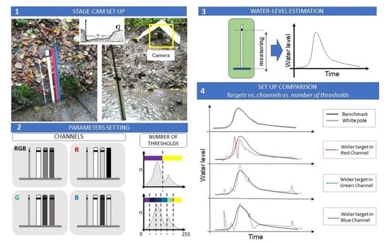
Funding

This study was supported by the European Research Council (ERC) DyNET project funded through the European Community’s Horizon 2020—Excellent Science—Programme (grant agreement H2020-EU.1.1.-770 999). Flavia Tauro acknowledges support by the “Departments of Excellence-2018” Program (Dipartimenti di Eccellenza) of the Italian Ministry of Education, University and Research, DIBAF-Department of University of Tuscia, Project “Landscape 4.0—Food, wellbeing and environment”.

Data Availability Statement

Conflicts of Interest

The authors declare no conflict of interest.

References

  1. Sarremejane, R.; Messager, M.L.; Datry, T. Drought in intermittent river and ephemeral stream networks. Ecohydrology 2022, 15, e2390. [Google Scholar] [CrossRef]
  2. Botter, G.; Durighetto, N. The stream length duration curve: A tool for characterizing the time variability of the flowing stream length. Water Resour. Res. 2020, 56, e2020WR027282. [Google Scholar] [CrossRef]
  3. Durighetto, N.; Vingiani, F.; Bertassello, L.E.; Camporese, M.; Botter, G. Intraseasonal drainage network dynamics in a headwater catchment of the Italian Alps. Water Resour. Res. 2020, 56, e2019WR025563. [Google Scholar] [CrossRef] [Green Version]
  4. Godsey, S.; Kirchner, J.W. Dynamic, discontinuous stream networks: Hydrologically driven variations in active drainage density, flowing channels and stream order. Hydrol. Process. 2014, 28, 5791–5803. [Google Scholar] [CrossRef]
  5. Botter, G.; Vingiani, F.; Senatore, A.; Jensen, C.; Weiler, M.; McGuire, K.; Mendicino, G.; Durighetto, N. Hierarchical climate-driven dynamics of the active channel length in temporary streams. Sci. Rep. 2021, 11, 21503. [Google Scholar] [CrossRef]
  6. Messager, M.L.; Lehner, B.; Cockburn, C.; Lamouroux, N.; Pella, H.; Snelder, T.; Tockner, K.; Trautmann, T.; Watt, C.; Datry, T. Global prevalence of non-perennial rivers and streams. Nature 2021, 594, 391–397. [Google Scholar] [CrossRef]
  7. Larned, S.T.; Datry, T.; Arscott, D.B.; Tockner, K. Emerging concepts in temporary-river ecology. Freshw. Biol. 2010, 55, 717–738. [Google Scholar] [CrossRef]
  8. Tauro, F.; Selker, J.; van de Giesen, N.; Abrate, T.; Uijlenhoet, R.; Porfiri, M.; Manfreda, S.; Caylor, K.; Moramarco, T.; Benveniste, J.; et al. Measurements and Observations in the XXI century (MOXXI): Innovation and multidisciplinarity to sense the hydrological cycle. Hydrol. Sci. J. 2018, 63, 169–196. [Google Scholar] [CrossRef] [Green Version]
  9. Constantz, J. Heat as a tracer to determine streambed water exchanges. Water Resour. Res. 2008, 44, W00D10. [Google Scholar] [CrossRef]
  10. Jensen, C.K.; McGuire, K.J.; McLaughlin, D.L.; Scott, D.T. Quantifying spatiotemporal variation in headwater stream length using flow intermittency sensors. Environ. Monit. Assess. 2019, 191, 226. [Google Scholar] [CrossRef]
  11. Paillex, A.; Siebers, A.R.; Ebi, C.; Mesman, J.; Robinson, C.T. High stream intermittency in an alpine fluvial network: Val Roseg, Switzerland. Limnol. Oceanogr. 2020, 65, 557–568. [Google Scholar] [CrossRef]
  12. Zimmer, M.A.; Kaiser, K.E.; Blaszczak, J.R.; Zipper, S.C.; Hammond, J.C.; Fritz, K.M.; Costigan, K.H.; Hosen, J.; Godsey, S.E.; Allen, G.H.; et al. Zero or not? Causes and consequences of zero-flow stream gage readings. Wiley Interdiscip. Rev. Water 2020, 7, e1436. [Google Scholar] [CrossRef] [PubMed]
  13. Kaplan, N.H.; Sohrt, E.; Blume, T.; Weiler, M. Monitoring ephemeral, intermittent and perennial streamflow: A dataset from 182 sites in the Attert catchment, Luxembourg. Earth Syst. Sci. Data 2019, 11, 1363–1374. [Google Scholar] [CrossRef] [Green Version]
  14. Pagano, S.G.; Sollitto, D.; Colucci, M.; Prato, D.; Milillo, F.; Ricci, G.F.; Gentile, F. Setting up of an experimental site for the continuous monitoring of water discharge, suspended sediment transport and groundwater levels in a mediterranean basin. Results of one year of activity. Water 2020, 12, 3130. [Google Scholar] [CrossRef]
  15. Vetra-Carvalho, S.; Dance, S.L.; Mason, D.C.; Waller, J.A.; Cooper, E.S.; Smith, P.J.; Tabeart, J.M. Collection and extraction of water level information from a digital river camera image dataset. Data Brief 2020, 33, 106338. [Google Scholar] [CrossRef]
  16. Perks, M.T.; Russell, A.J.; Large, A.R.G. Technical Note: Advances in flash flood monitoring using unmanned aerial vehicles (UAVs). Hydrol. Earth Syst. Sci. 2016, 20, 4005–4015. [Google Scholar] [CrossRef] [Green Version]
  17. Pearce, S.; Ljubičić, R.; Peña-Haro, S.; Perks, M.; Tauro, F.; Pizarro, A.; Dal Sasso, S.F.; Strelnikova, D.; Grimaldi, S.; Maddock, I.; et al. An evaluation of image velocimetry techniques under low flow conditions and high seeding densities using Unmanned Aerial Systems. Remote Sens. 2020, 12, 232. [Google Scholar] [CrossRef] [Green Version]
  18. Birgand, F.; Chapman, K.; Hazra, A.; Gilmore, T.; Etheridge, R.; Staicu, A.M. Field performance of the GaugeCam image-based water level measurement system. PLoS Water 2022, 1, e0000032. [Google Scholar] [CrossRef]
  19. Noto, S.; Tauro, F.; Petroselli, A.; Apollonio, C.; Botter, G.; Grimaldi, S. Low-cost stage-camera system for continuous water-level monitoring in ephemeral streams. Hydrol. Sci. J. 2022, 67, 1439–1448. [Google Scholar] [CrossRef]
  20. Tauro, F.; Tosi, F.; Mattoccia, S.; Toth, E.; Piscopia, R.; Grimaldi, S. Optical Tracking Velocimetry (OTV): Leveraging Optical Flow and Trajectory-Based Filtering for Surface Streamflow Observations. Remote Sens. 2018, 10, 2010. [Google Scholar] [CrossRef]
  21. Tosi, F.; Rocca, M.; Aleotti, F.; Poggi, M.; Mattoccia, S.; Tauro, F.; Toth, E.; Grimaldi, S. Enabling image-based streamflow monitoring at the edge. Remote Sens. 2020, 12, 2047. [Google Scholar] [CrossRef]
  22. Livoroi, A.H.; Conti, A.; Foianesi, L.; Tosi, F.; Aleotti, F.; Poggi, M.; Tauro, F.; Toth, E.; Grimaldi, S.; Mattoccia, S. On the Deployment of Out-of-the-Box Embedded Devices for Self-Powered River Surface Flow Velocity Monitoring at the Edge. Appl. Sci. 2021, 11, 7027. [Google Scholar] [CrossRef]
  23. Adrian, R.J. Particle-imaging techniques for experimental fluid-mechanics. Annu. Rev. Fluid Mech. 1991, 23, 261–304. [Google Scholar] [CrossRef]
  24. Tauro, F.; Piscopia, R.; Grimaldi, S. PTV-Stream: A simplified particle tracking velocimetry framework for stream surface flow monitoring. Catena 2019, 172, 378–386. [Google Scholar] [CrossRef]
  25. Otsu, N. A threshold selection method from gray-level histograms. IEEE Trans. Syst. Man Cybern. 1979, 9, 62–66. [Google Scholar] [CrossRef]
Figure 1. Experimental setup including: white pole, three colored bars, and a wildlife camera.
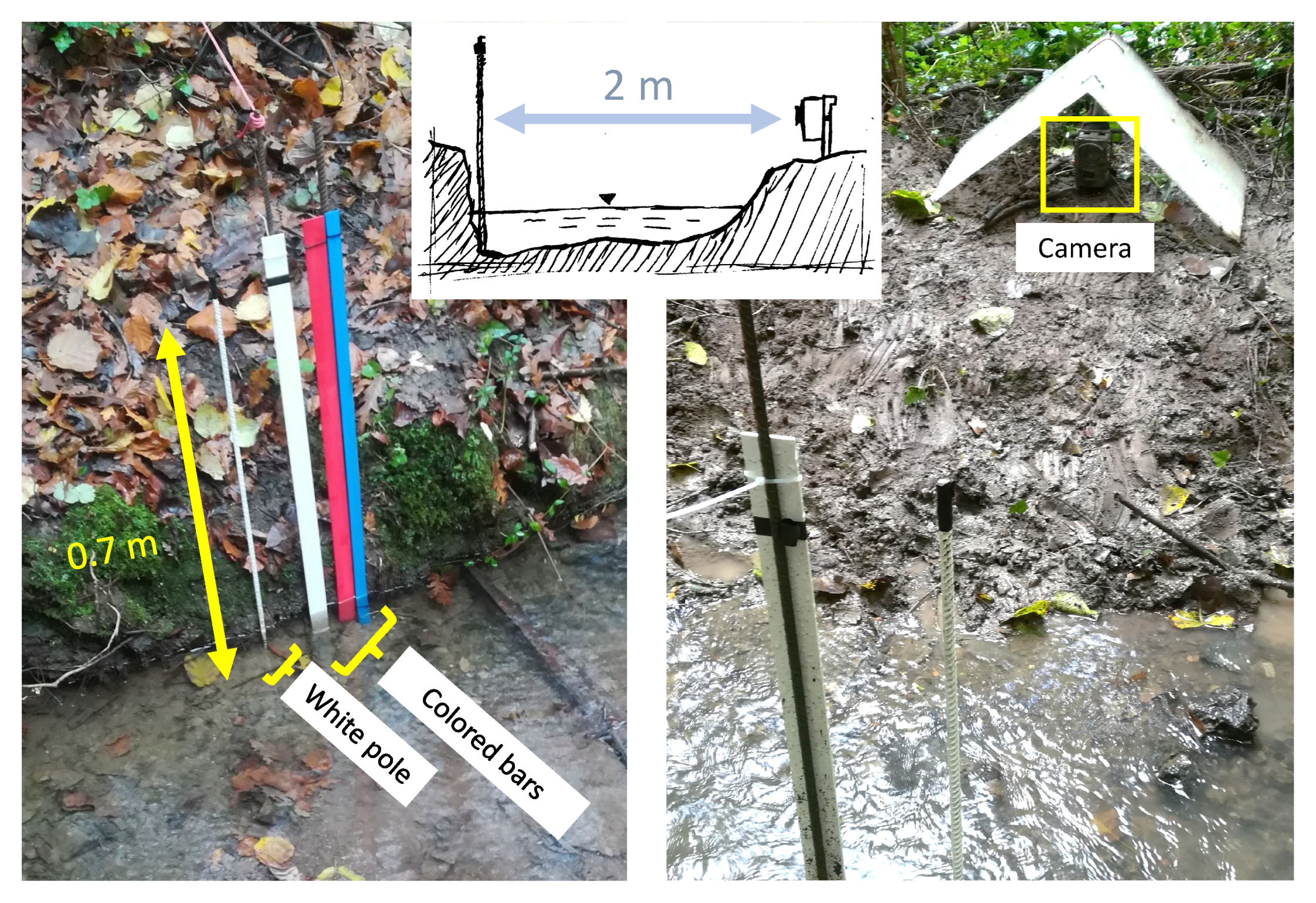
Remotesensing 14 06064 g001
Figure 2. Unfiltered (left) and filtered (right) water levels computed from the pole and the white bar for experimental tests E1 and E5–E7. Benchmark water levels are in green markers and transparent black; pole unfiltered and filtered in dashed and solid blue, respectively; and white bar unfiltered and filtered in dashed and solid red, respectively. Light gray vertical bars indicate NIR frames.
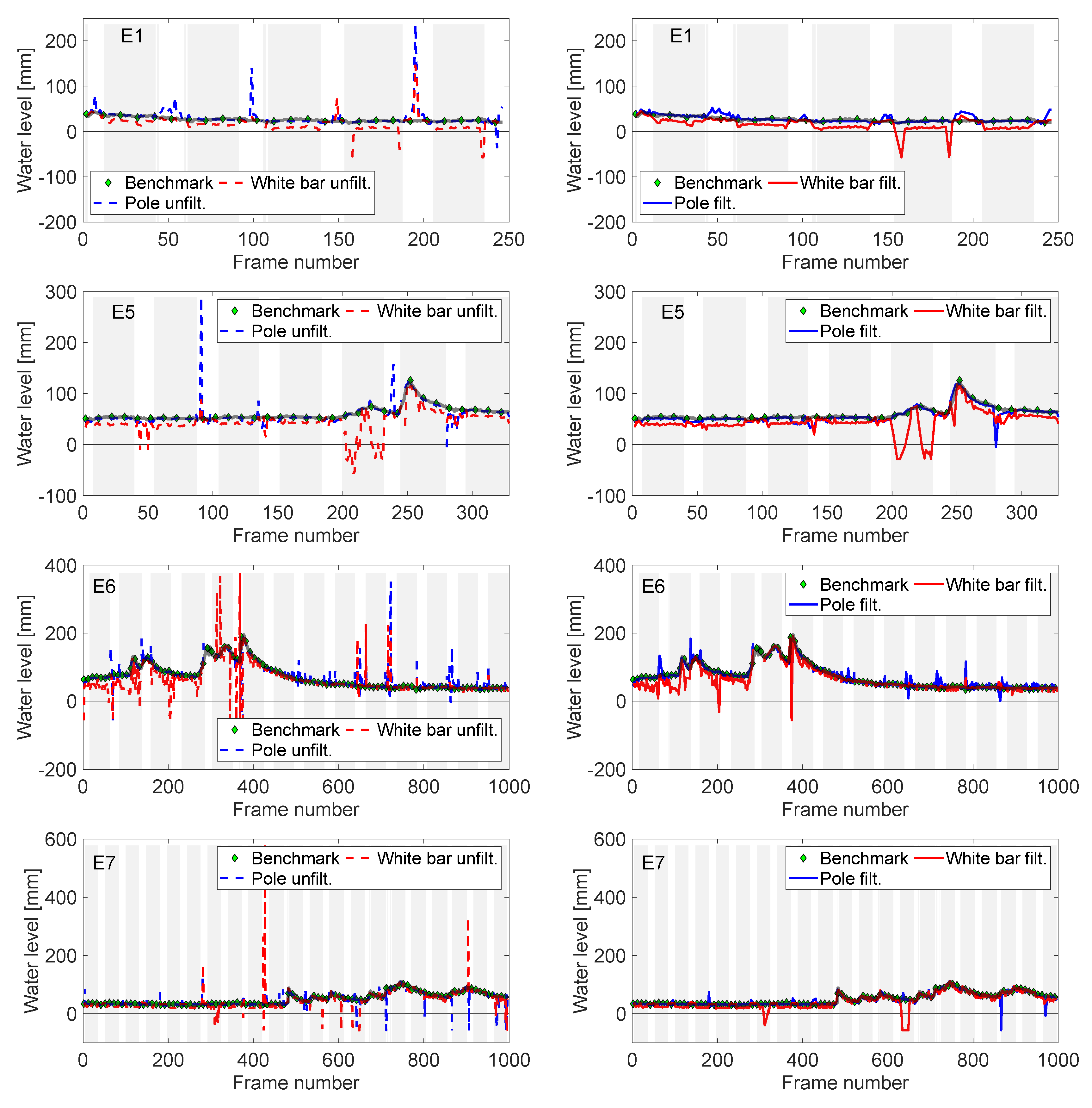
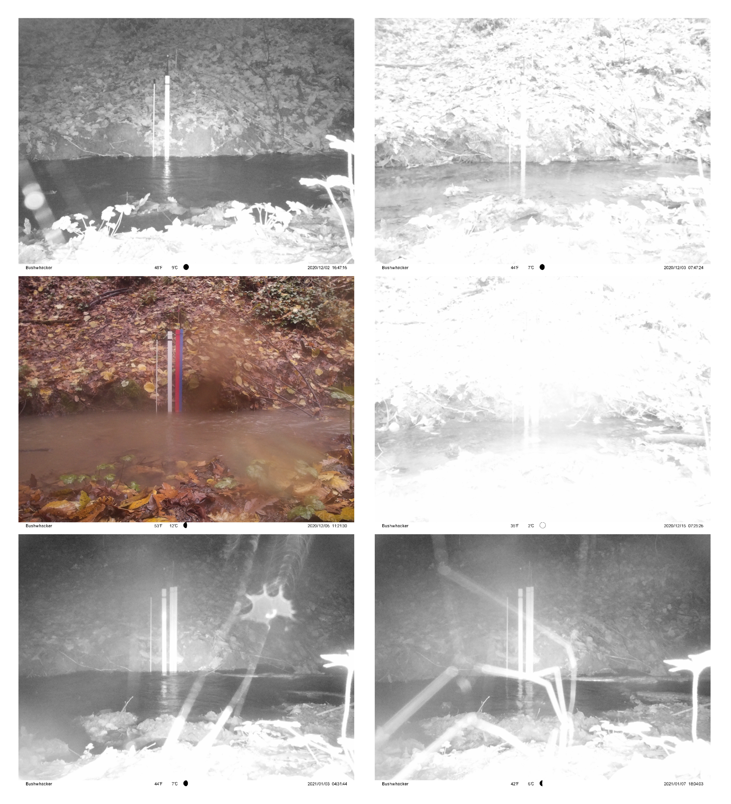
Remotesensing 14 06064 g002
Figure 3. Examples of good-quality (left) and poor-quality (right) images taken during experiments E5–E7 (from top to bottom). Right-side pictures led to large deviations from the benchmark.
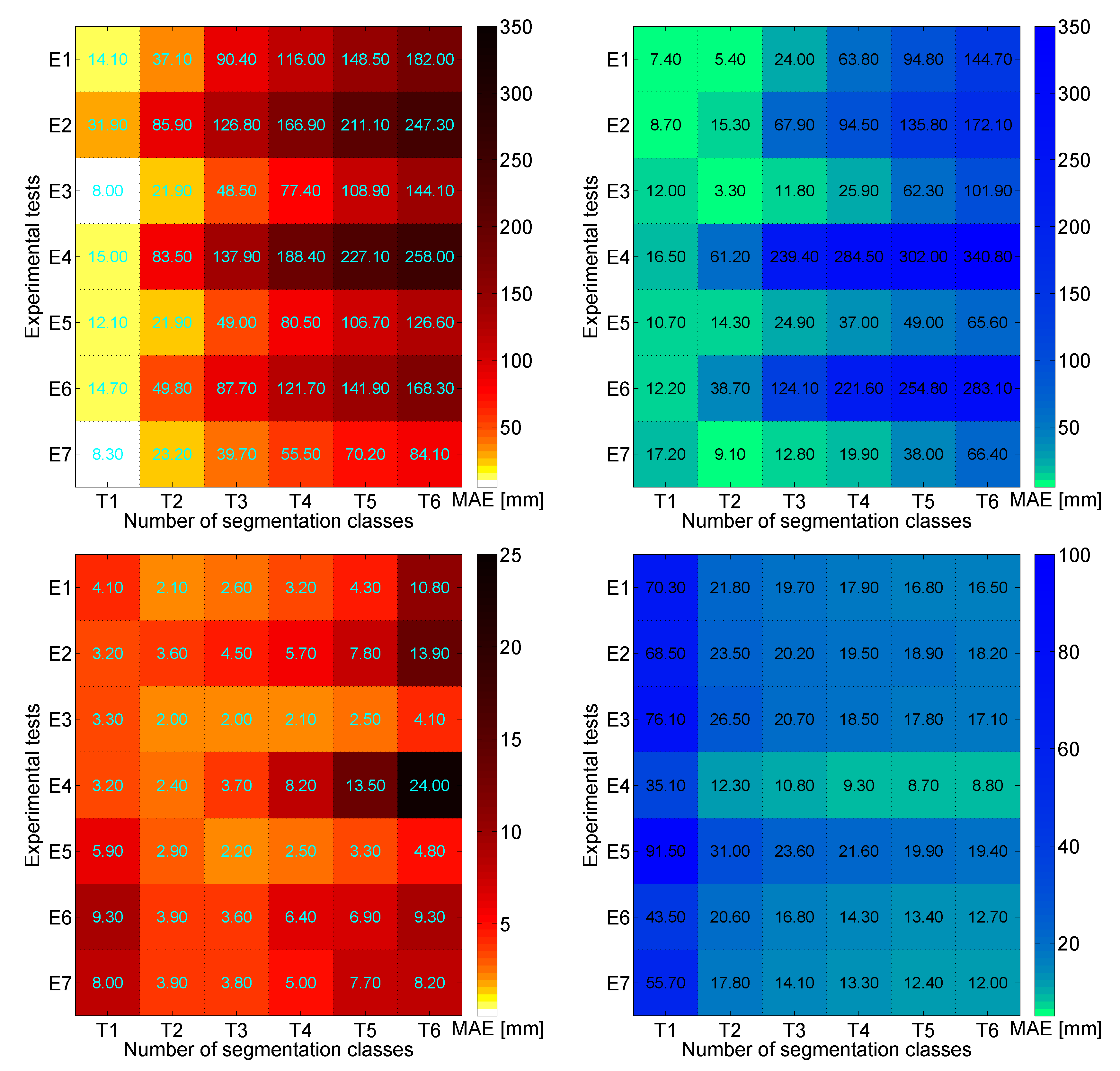
Remotesensing 14 06064 g003
Figure 4. Mean absolute error (MAE) in mm between unfiltered and a priori known pole/white bar lengths for all experimental tests (E1 to E7). Left side heatmaps show values estimated from images of the pole in RGB (top) and NIR (bottom). Right side heatmaps show values estimated from images of the white bar in RGB (top) and NIR (bottom). Values are reported for all segmentation classes (T1 to T6).
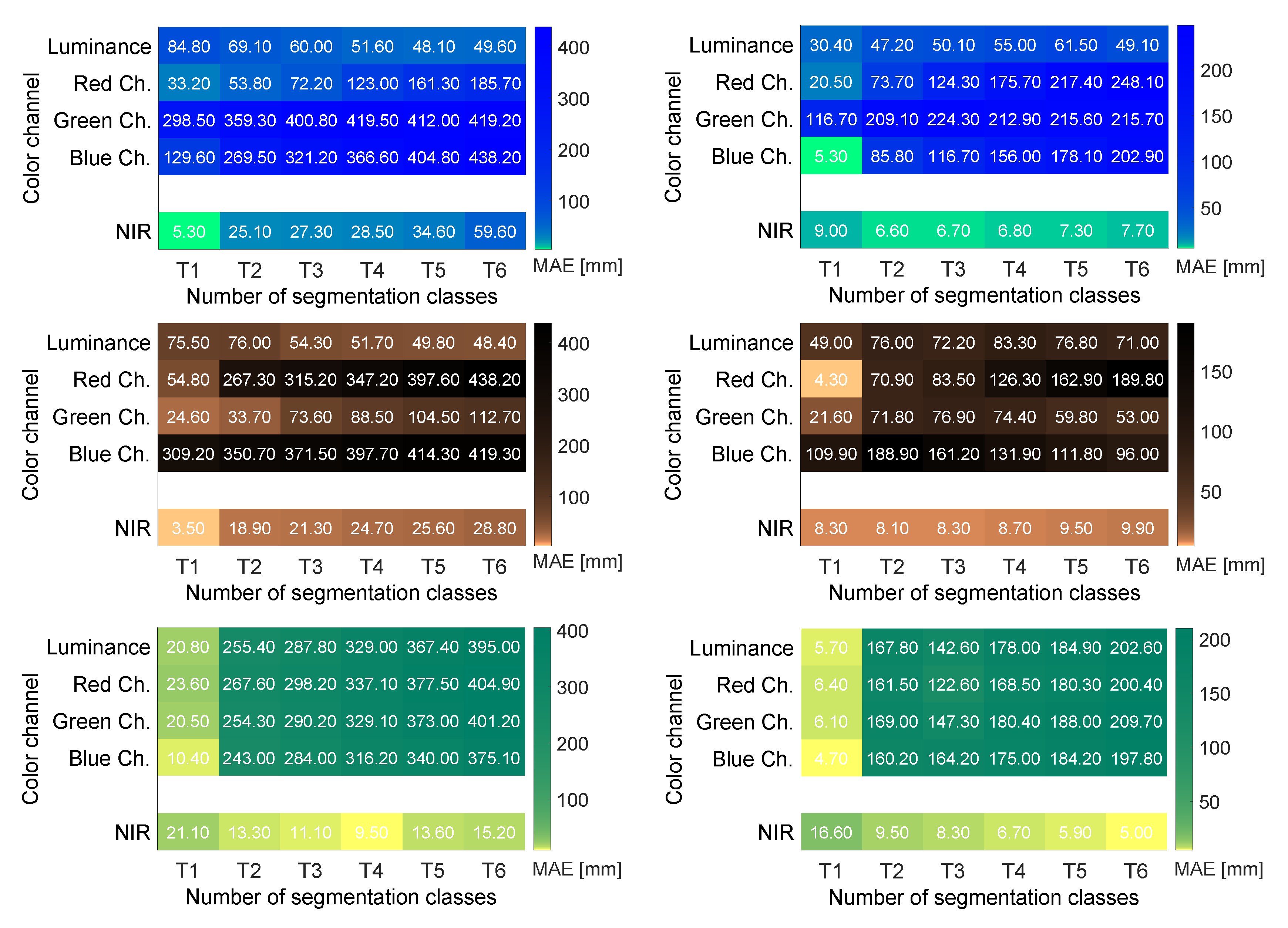
Remotesensing 14 06064 g004
Figure 5. Mean absolute error (MAE) in mm between unfiltered and a priori known bar lengths for all experimental tests (E6, left, and E7, right) treated with the narrow image crop. From top to bottom, heatmaps show MAE values estimated from images of the blue (top), red (middle), and white (bottom) bars. In each heatmap, rows indicate MAEs obtained for different color channels: the top four rows report values for RGB images processed through four gray-scale conversion modalities (luminance, red, green, and blue channels). The bottom row refers to values for NIR images. Values are reported for all segmentation classes (T1 to T6).
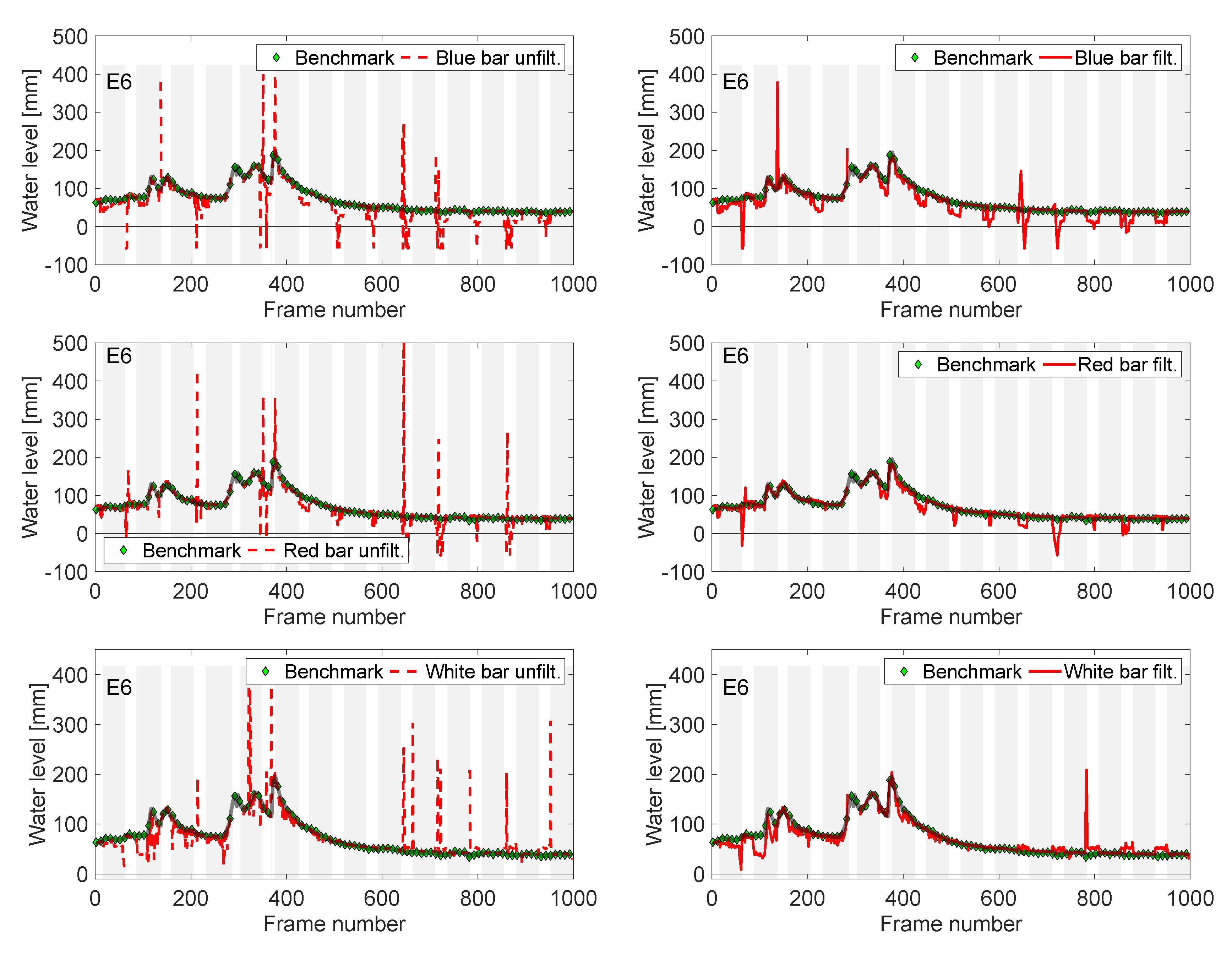
Remotesensing 14 06064 g005
Figure 6. Raw (left) and filtered (right) water levels computed from the bars (top: blue, middle: red, bottom: white) for experimental test E6. Benchmark water levels are in green markers and transparent black; bar raw and filtered in dashed and solid red, respectively. Light gray vertical bars indicate NIR frames. Images are treated with the narrow image crop.
Remotesensing 14 06064 g006
Figure 7. Mean absolute error (MAE) in mm between unfiltered and a priori known bar lengths for all experimental tests (E6, left, and E7, right) treated with the large image crop. From top to bottom, heatmaps show MAE values estimated from images of the blue (top), red (middle), and white (bottom) bars. In each heatmap, rows indicate MAEs obtained for different color channels: the top four rows report values for RGB images processed through four gray-scale conversion modalities (luminance, red, green, and blue channels). The bottom row refers to values for the NIR images. Values are reported for all the segmentation classes (T1 to T6).
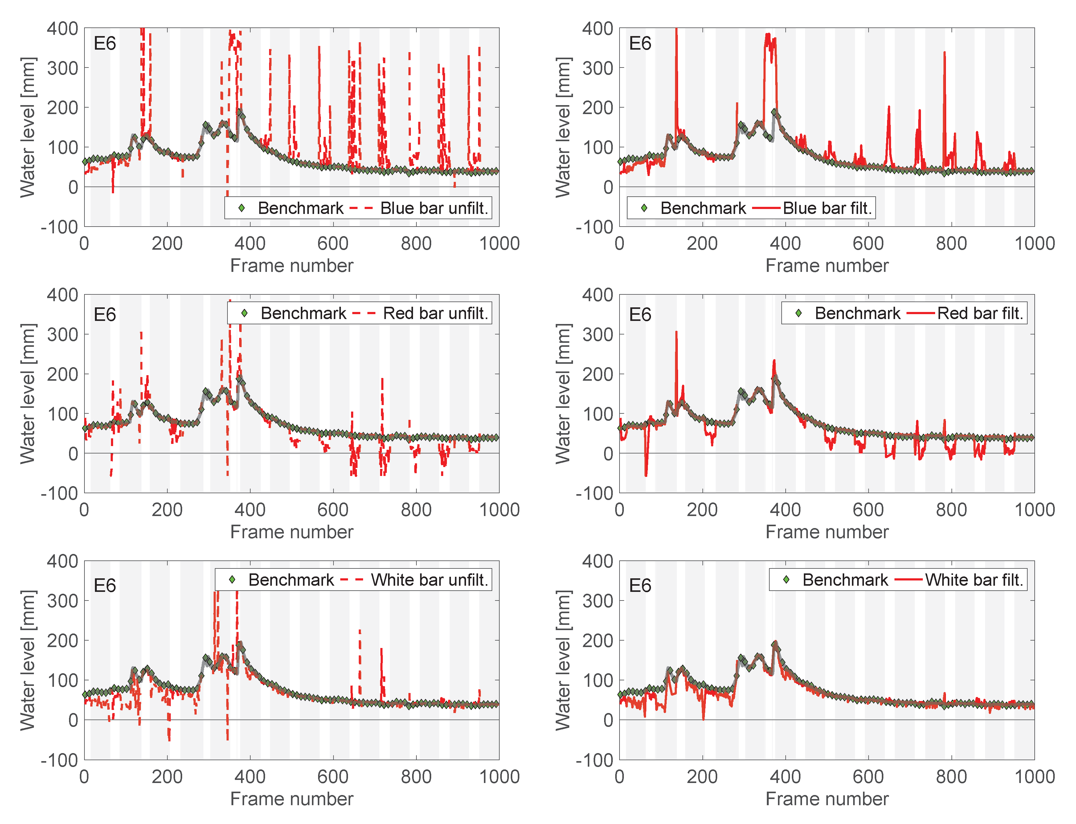
Remotesensing 14 06064 g007
Figure 8. Raw (left) and filtered (right) water levels computed from the bars (top: blue, middle: red, bottom: white) for experimental test E6. Benchmark water levels are in green markers and transparent black; bar raw and filtered in dashed and solid red, respectively. Light gray vertical bars indicate NIR frames. Images are treated with the large image crop.
Remotesensing 14 06064 g008
Table 1. Initial and final dates, times, and number of frames for the experimental tests.
TestInitial Date and TimeFinal Date and TimeNumber of Frames
E12020/10/15 10:402020/10/20 14:45249
E22020/10/20 15:202020/10/29 10:20423
E32020/10/29 11:202020/11/06 13:20389
E42020/11/17 11:302020/11/27 11:30481
E52020/11/27 12:162020/12/04 09:15331
E6A2020/12/04 11:002020/12/08 09:00283
E6B2020/12/08 18:002020/12/18 07:00690
E72020/12/18 14:002021/01/08 09:301000
Table 2. Light conditions during each experimental test. Abbreviations “morn.” and “aft.” stand for morning and afternoon, respectively. The index G quantifies the average intensity of gray-scale images captured during the day.
TestLight ConditionsG
E1Diffused sunlight in morn. and aft.; weakly scattered in the day83
E2Diffused sunlight in morn. and aft.; weakly scattered in the day86
E3Diffused sunlight in morn. and aft.; weakly scattered in the day90
E4Diffused sunlight in early morn. and aft.; scattered in the day93
E5Diffused sunlight in early morn. and aft.; scattered in the day95
E6Diffused sunlight in morn. and aft.; weakly scattered in the day104
E7Diffused sunlight in early morn. and aft.; scattered in the day101
Table 3. Rainfall characteristics (I, average intensity, and duration) for experimental tests executed during the precipitation events.
TestRainfall Event Initial Date and TimeI [mm/h]Duration [min]
E22020/10/24 07:304.880
2020/10/26 21:504.650
E42020/11/20 05:403.230
2020/11/20 07:103.2260
E52020/12/01 16:203.020
2020/12/01 19:001.6120
2020/12/01 23:102.170
2020/12/02 10:303.3450
E62020/12/05 04:401.7120
2020/12/05 13:101.950
2020/12/05 22:205.0240
2020/12/06 06:303.4330
2020/12/06 13:105.550
2020/12/07 03:402.140
2020/12/07 07:402.030
2020/12/08 01:003.6630
2020/12/08 17:402.4250
2020/12/08 23:202.780
2020/12/09 03:401.460
2020/12/09 12:307.260
2020/12/09 21:402.030
2020/12/10 07:302.830
E72020/12/28 07:202.470
2020/12/28 11:404.7160
2020/12/28 15:402.3110
2020/12/29 14:304.280
2020/12/29 17:402.660
2020/12/30 04:001.540
2020/12/30 10:502.830
2020/12/30 13:404.790
2021/01/01 09:002.7220
2021/01/01 15:202.430
2021/01/02 03:302.250
2021/01/02 05:503.5140
2021/01/02 10:202.6210
2021/01/02 20:103.860
2021/01/03 02:403.650
2021/01/03 14:201.2100
2021/01/04 16:401.840
2021/01/05 05:502.1120
2021/01/05 11:303.680
2021/01/05 23:101.9180
2021/01/07 00:203.620
Table 4. Optimal number of segmentation classes for RGB ( T RGB ) and NIR ( T NIR ) images.
TestPoleWhite Bar
T RGB T NIR T RGB T NIR
E11226
E21116
E31326
E41215
E51316
E61316
E71326
Table 5. MAE in mm between filtered and benchmark lengths estimated from the entire sequence of RGB and NIR images for the pole and white bar.
TestPoleWhite Bar
mm mm
E14.411.4
E29.313.7
E32.611.2
E43.06.7
E53.815.8
E65.89.8
E73.78.9
Table 6. Optimal combinations of gray-scale conversion modality (red, green, and blue channel, ch.) and number of segmentation classes ( T RGB and T NIR for RGB and NIR, respectively) for each bar (blue, red, and white) and experimental test (E6 and E7). Images are treated with the narrow crop.
BarE6E7
T RGB T NIR T RGB T NIR
BlueRed Ch. − 11Blue Ch. − 12
RedGreen Ch. − 11Red Ch. − 12
WhiteBlue Ch. − 14Blue Ch. − 16
Table 7. MAE in mm between benchmark and filtered lengths estimated from the entire sequence of RGB and NIR images of the colored and white bars treated with the narrow crop.
BarE6E7
MAE MAE
mm mm
Blue11.84.5
Red7.05.6
White7.03.9
Table 8. Optimal combinations of gray-scale conversion modality (red, green, and blue channel, ch.) and number of segmentation classes ( T RGB and T NIR for RGB and NIR, respectively) for each bar (blue, red, and white) and experimental test (E6 and E7). Images are treated with the large crop.
BarE6E7
T RGB T NIR T RGB T NIR
BlueBlue Ch. − 12Blue Ch. − 14
RedGreen Ch. − 52Red Ch. − 12
WhiteBlue Ch. − 16Blue Ch. − 26
Table 9. MAE in mm between benchmark and filtered lengths estimated from the entire sequence of RGB and NIR images of the colored and white bars treated with the large crop.
BarE6E7
MAEMAE
mmmm
Blue17.98.6
Red11.29.9
White8.68.9
Publisher’s Note: MDPI stays neutral with regard to jurisdictional claims in published maps and institutional affiliations.

