Monitoring Shoreline Changes along the Southwestern Coast of South Africa from 1937 to 2020 Using Varied Remote Sensing Data and Approaches

Abstract

Shoreline analysis in response to the rapid erosion of sandy beaches has evolved along with geospatial and computer technology; it remains an essential task for sustainable coastal management. This severe and rapid erosion has been reported at several sandy beaches worldwide, including Yzerfontein beaches, on the southwest coast of South Africa. We determined this vulnerability from 1937 to 2020 and predicted its change by 2040 by manually delineating shoreline positions from 1937, 1960, and 1977 from aerial photographs and Landsat products between 1985 and 2020 in an automated fashion using the CoastSat toolkit and Google Earth Engine. We then integrated these datasets to calculate the extent of shoreline dynamics over the past eight decades using the Digital Shoreline Analysis System (DSAS). Our results show that the coastline changed dynamically between 1937 and 2020, culminating in an average net erosion of 38 m, with the most extensive erosion occurring between 2015 and 2020. However, coastal projections indicate a slight change in shoreline position over the next two decades. Further studies should integrate additional high resolution remote sensing data and non-remote sensing data (e.g., field surveys) to improve our results and provide a more thorough understanding of the coastal environment and overcome some of remotely-sensed data underlying uncertainties.

1. Introduction

Coastal erosion is increasingly becoming a public issue and is no longer just a problem for coastal managers. Instead, it is a universal problem that affects almost every country with a coastline [1]. Furthermore, it is often associated with the discrete or combined interaction of naturally induced mechanisms such as storms, sediment fluxes and human-induced activities such as infrastructure development and sand mining [2,3]. The consequences of coastal erosion include loss of life, disruption of economic sectors, and degradation of coastal ecosystems and biodiversity [4]. Therefore, to protect coastal infrastructure and its socio-economic potential, it is necessary to monitor coastal areas actively and evaluate their time-space patterns [5]. While coastal erosion is exacerbated by climate-driven sea level rise and anthropogenic forces, the extent and severity vary from region to region.

The threat of coastal erosion is widespread on sandy coasts, and the destruction of coastal infrastructure and ecosystems is increasingly reported [2,6,7,8]. For example, Hinkel et al. [6] estimated a loss of nearly 6,000 to 17,000 km² of land due to increased coastal erosion associated with sea-level rise and other factors, while Vousdoukas et al. [8] projected a more drastic prospect of the near-elimination of nearly half of the world’s sandy beaches by the end of the 21st century. However, coastal environments are inherently dynamic and modelling sea-level rise risks and coastal morphology needs to be site-specific and substantiated with an appropriate range of data [9]. These results underscore the need to understand patterns that cause coastal erosion and pose a global risk to coastal communities.

This threat to coastal communities is a severe issue for countries such as South Africa, where 80% of the 3000 km coastline consists of sandy beaches; thus, much of the country’s coastal developments and ecosystems could be at increased risk of destruction from coastal erosion [10,11]. In addition, South Africa’s coastal resources contribute nearly USD 6.3 billion to national income [12]; thus, the potential damage has socio-economic implications for the country. This problematic situation has been reported at several sandy beaches in South Africa, for example, near the Cape Town [13]. Moreover, this part of South Africa is subject to violent frontal storms, such as the ‘Cape Storm’ of June 2017, which brought extreme winds, rain, significant swell waves and storm surges that caused extensive damage to infrastructure and eroded stretches of the region’s coastline, including Sixteen Mile Beach [14,15].

Sustainable coastal management requires active, cost-effective, and consistent mapping of shorelines to implement proactive planning strategies for coastal resource protection and management [16]. One promising and practical method is extracting shoreline features from digital remote-sensing imagery [17]. Remote sensing with improved sensor technology, open access data policies, and near real-time data collection has the unique advantage of providing geographically unrestricted information at a lower cost than traditional ground-based monitoring [18]. For more than four decades, remote sensing has contributed immensely to coastal monitoring by providing timely and affordable information at multiple geographic scales [7]. In addition, its capabilities provide a unique view into the past to observe shoreline dynamics over time and to use these historical data to model possible future shoreline changes.

Various remote sensing products have been used successfully to monitor shoreline changes in different parts of the world. For example, Choung et al. [19] used light detection and ranging (LiDAR) data to map shoreline changes in the United States with great thematic fidelity. Cabezas-Rabadán et al. [20] characterized short-term beach dynamics in Spain with Sentinel-2 imagery. Maglione et al. [21] used high-resolution WorldView-2 imagery to extract coastline modifications. Wang et al. [22] studied the spatio-temporal changes of Ningbo coasts between 1976 and 2015 using Landsat sensors and their results showed an increased mean Net Shoreline Movement (NSM) from 187 m to 298 m, with the mean annual NSM reaching 85 m/year, indicating the progress of the coasts towards the sea. Xu [23] used nearly three decades of Landsat data (1986–2015) to analyze the coast of the US State of Texas and found that it endured changes at a rate of −0.154 ± 0.063 km²/year, with 52.58% of the total coastline retreated the land, while 47.42% encroached the sea. Specht et al. [24] analyzed the coastal variability in Sopot based on Landsat satellite data and found an average coastline shift of 19.1 m towards the sea between 2008 and 2018. More recently, Mao et al. [25] mapped shoreline changes using Landsat data within the Google Earth Engine (GEE) scalable cloud computing platform. Landsat is advantageous for monitoring long-term shoreline changes due to its longevity and open access [26]. Furthermore, its full archive is publicly available in the GEE with various geospatial data processing functions [22], empowering users to efficiently import and analyze data without the burden of storing and processing data in local computers [27]. Despite these resources, until now, no detailed analysis of long-term coastal change has been conducted on the west coast of South Africa, particularly at Yzerfontein and Sixteen Mile Beach. This article attempts to fill this gap.

Given the challenging context for coastal areas, we aim to analyze temporal-spatial coastline dynamics at Yzerfontein and Sixteen Mile Beach between 1937 and 2020 and to forecast future shoreline changes. To achieve this goal, we manually delineated coastline positions from 1937, 1960, and 1977 on aerial photographs and Landsat products from 1985 to 2020 using the CoastSat toolkit and GEE in an automated fashion. We then integrated these datasets to calculate the extent of shoreline dynamics over the past eight decades using the Digital Shoreline Analysis System (DSAS) and predict changes over the next two decades.

In the next section, we describe the coastal area in which the study was conducted and clarify the datasets and methodological framework used to understand coastal change in the area studied. We then present the results based on five statistical variables: Net Shoreline Movement (NSM), Shoreline Change Envelope (SCE), End Point Rate (EPR), and Linear Regression Rate (LRR), Weighted Linear Regression (WLR) and predict the potential shoreline changes in the next 10 and 20 years. After discussion, limitations are identified and the potential for future research is suggested before conclusions are drawn.

2. Materials and Methods

2.1. Description of the Study Site

The study sites cover a 30 km stretch of South Africa’s southwestern coastline situated around the West Coast National Park and the small town of Yzerfontein (33°20′50″S; 18°08′60″E), which is approximately 80 km north of Cape Town in the Western Cape Province (Figure 1). The coastline is microtidal, with a monthly range of about 1.8 m. It is noteworthy, that unlike many of the other bays on the western coast, Yzerfontein presently has no local riverine input of sediment. All sandy sediment, marine and aeolian, is derived from the south by a combination of longshore drift and the prevailing strong southerly summer winds moving sand from exposed beaches further south. Dassen Island, the rocky Yzerfontein point and the harbour breakwater, which was extended in the 1980s, shelter the Yzerfontein Main Beach to some extent from the southerly marine swell. The Meeurots islet in the middle of the bay and the rocky point Rooipan se Klippe (or Gabbro Point) at the northern end of Yzerfontein Main Beach complicate the refraction and diffraction of the incoming waves, which in turn may affect the wave energy reaching different parts of the shore. The energy of incoming waves is high, with swells that routinely reach 5–6 m and sometimes up to 12 m in rare extreme storms. Storms and rainfall are more common in winter with this region having a semi-arid Mediterranean climate, with dry, warm summers and cool, wet winters [28].

This coastline comprises three different sandy beaches, the main areas under investigation: Sixteen Mile Beach, Yzerfontein Main Beach, immediately to the north of the town, and Pearl Bay to the south of the town.

2.1.1. Yzerfontein Main Beach

Yzerfontein was established as a town in 1937 when portions of coastal farmland were cleared for development [29]. Over the decades, the area has developed into a small town of more than 1500 residents, with tourism and second-home construction as its main attractions [30]. It stretches 800 m from the harbor and rocky headland, on which most of the town is built, to the small rock outcrop of Gabbro Point (marked as ‘Rooipan se Klippe’ on topocadastral maps). It is a gently sloping, fine-grained beach about 60 m wide. Half of the beach is backed by the public access car park, while a small, protected dune cordon backs the other half, opposite the town’s caravan park. Out to sea, there is another rock outcrop called Meeurots, which, in conjunction with the harbor seawall, dissipates some of the wave energy before it reaches the beach.

2.1.2. Pearl Bay

Pearl Bay is the name given to the southern and newer extension of Yzerfontein, where luxury holiday home developments have steadily grown since the early 2000s [30]. This coastal strip stretches 3.5 km from Schaapen Island to the town’s southern edge. Pearl Bay consists of four smaller embayments around various rock outcrops. Here, we group these smaller beaches as Pearl Bay. They have a slightly steeper profile, backed by partially vegetated dunes with increasing numbers of newly built houses.

2.1.3. Sixteen Mile Beach

Sixteen Mile Beach is one of the longest uninterrupted sandy beaches in South Africa, and much of it is located within the West Coast National Park (WCNP) and Marine Protected Area. The park was officially proclaimed in 1985 to protect and conserve the unique and ecologically sensitive Langebaan Lagoon and surrounding coastal fynbos ecosystems [31].

2.2. Remote Sensing Data

2.2.1. Aerial Photography

We obtained historical aerial photographs from the National Geospatial Information Agency (NGI), a division of the South African Department of Rural Development and Land Reform [32]. These historical aerial photographs are scanned, black-and-white images with their associated flight paths that reference the images’ date, time, elevation, coverage, and ground scale. Data selection was based on the availability of photographs and complete coverage of the study area, resulting in three selected periods: 1937, 1960 and 1977 (

Table 1. Summary of the historical aerial photographs data.

Year	Month	Scale	Number of Photographs
1937	April	1:22,000	11
1960	December	1:36,000	6
1977	March	1:60,000	3

).

The aerial photographs were rectified and georeferenced to align with a sub-meter high-resolution Maxar Technologies^© ESRI online satellite imagery base map projected to WGS 1984 UTM Zone 34 South. This map projection is the most appropriate for this region [33]. Suitable ground control points were identified for the entire study area before georeferencing and matched to the aerial photographs and transformed using a second-order polynomial transformation which also decreased any distortions within the images such as tilt, lens distortion and relief displacement. The same base image and similarly positioned ground control points were used throughout the georectification process to decrease the error and to ensure that the results could be comparable. Overall, each of the 20 aerial photographs had total root mean square error terms (RMSE) averaging less than 3 m. The georeferenced images were then cropped and mosaicked together to create a continuous single 8-bit unsigned raster for each of the three time periods, covering the entire stretch of the study site shoreline.

2.2.2. Landsat Imagery

The initial step to acquiring the satellite imagery data was to link the CoastSat Python toolkit to an existing GEE account to access its vast cloud-storage of remote sensing data. Then, the entire Landsat 5, 7 and 8 products were accessed, and the selected data were downloaded using CoastSat within GEE based on the user-defined parameters such as the study period, the satellite mission and study area geometry (CoastSat is further explained in Section 2.3.2). Next, the Landsat data were sampled at 5-year intervals (

Table 2. Landsat image selection dates for the shoreline analysis.

Year	Acquisition Date	Satellite Mission
1985	9 April	Landsat 5
1990	19 December	Landsat 5
1995	30 October	Landsat 5
2000	20 November	Landsat 7
2005	9 October	Landsat 5
2010	29 March	Landsat 5
2015	22 November	Landsat 8
2020	9 October	Landsat 8

) to capture the medium-term variation of the shoreline from 1985 to 2020. Only one image acquisition date was selected from the specified years; this was based on various criteria; the main being cloudless imagery, as clouds may affect the classification and shoreline position detection, and hence images acquired in summer months (October to March) because the studied area has a Mediterranean climate.

2.3. Shoreline Change Detection

2.3.1. Shoreline Extraction from Aerial Photographs

Shorelines were extracted from aerial photographs and Landsat; therefore, it is instructive to explain the processes separately. The overall methodological framework and objectives of this study are presented in Figure 2.

We first delineated the shoreline position from the aerial photographs using the High Water Line (HWL) as the main shoreline indicator. This marks the extent of the previous high tide and is indicated by the dark grey boundary in the sand from where the water has decreased the sand’s reflectance of light [34]. The most common method of marking this indicator is manually digitizing the water-land boundary, which is considered the simplest delineation technique when working with non-extensive study sites [35]. The HWL is also the more appropriate indicator to use for micro-tidal environments, such as Yzerfontein. Thus, the HWL was digitized by carefully tracing the visible grey boundary features on the georeferenced aerial photographs.

As Hapke et al. [36] noted, every time a shoreline position is delineated from a remotely sensed data source or a field survey, it will always contain an associated error or uncertainty in its position. These errors include human error (or bias) when manually digitizing, sensor distortions, georeferencing errors, the errors associated with the image’s scale or pixel size, and external effects of the tidal cycle [37]. Moreover, most calculations for uncertainty follow a similar equation, which is the square root of the sum of squares for different variables that affect the shoreline’s position; they represent the horizontal distance within which the shoreline could be located [36,38] (Equation (1)):

$$U=\sqrt{E_g^{ 2}+E_p^{ 2}+E_d^{ 2} }$$

(1)

where E_g is the georeferencing error, which is the average total Root Mean Square Error (RMSE) for all the images. E_p is the pixel error, which is the minimum pixel size for the image based on its scale. E_d is the digitization error, which can be approximated by at least half the pixel size. These variables result in total horizontal uncertainty values of 4.09, 5.13 and 6.05 m for the three respective time periods (see

Table 3. Estimated total shoreline uncertainty for each of the historical aerial photographs.

Measurement Uncertainty (m)	1937	1960	1977
Georeferencing error (Eg) (Average Total RMSE)	2.35	2.52	2.32
Pixel error (Ep)	3.00	4.00	5.00
Digitization error (Ed)	1.50	2.00	2.50
Total shoreline uncertainty (U)	4.09	5.13	6.05

).

2.3.2. CoastSat Shoreline Extraction

We also extracted shorelines using the novel open-source software CoastSat, which operates in an online Python coding visualization environment (Jupyter Notebook) and uses Google Earth Engine (GEE) and supervised image classification techniques to automatically extract the shoreline position from all publicly available Landsat imagery [39]. The first step is to discriminate water features in contrast with terrestrial land features, which McFeeters [40] achieved through the Modified Normalized Difference Water Index (MNDWI) calculated from the shortwave infrared and visible green regions of the electromagnetic spectrum (Equation (2)):

$$MNDWI=\frac{SWIR-Green}{SWIR+Green}$$

(2)

where Green is the reflectance of green band and SWIR is the reflectance of shortwave infrared (SWIR) band of the Landsat imagery. CoastSat uses a combination of a neural network supervised classification, the MNDWI and Otsu’s threshold algorithm to detect the shoreline position [39,41]. In addition, Otsu’s thresholding algorithm was applied to identify the maximum variance between the sand and water classes. CoastSat performs optimally with smaller study areas (e.g., 5 km²), and it is recommended that broader study areas (e.g., 100 km²) are divided into sub-areas to handle the data computations better [36]. For this reason, we divided the 30 km stretch of coastline into four parts, and the code was run four times per period. After classification and shoreline delineation, we visually inspected and approved that there were no major misclassifications or incorrectly placed shoreline positions due to cloud cover. Next, the four sub-areas were merged to form one continuous shoreline in the study site for each image date (8 and 304, respectively). Finally, the vector polylines were clipped to remove all the rock outcrops, such as Gabbro Point, Yzerfontein Point, Schaapen Island and Bakoond, leaving only the sandy beaches.

Similar aerial photographs and satellite-derived shorelines also contain a positional uncertainty (U) based on the satellite imagery geo-accuracy (georeferencing; E_g) and pixel size (E_p) [39]. Therefore, the total horizontal uncertainty (Equation (3)) follows the same formula as Equation (1) but does not include a digitization error. Every Landsat image contains a geometric RMSE value in its metadata, and

Table 4. Estimated total shoreline uncertainty for each of the Landsat images.

Measurement Uncertainty (m)	1985	1990	1995	2000	2005	2010	2015	2020
Georeferencing error (Eg) (RMSE)	5.18	8.06	5.07	6.15	5.68	4.99	8.88	7.43
Pixel error (Ep)	15.0	15.0	15.0	15.0	15.0	15.0	15.0	15.0
Total shoreline uncertainty (U)	15.87	17.02	15.83	16.21	16.04	15.81	17.43	16.74

summarizes these error values.

$$Landsat U=\sqrt{E_g^{ 2}+E_p^{ 2}}$$

(3)

2.4. Long-Term Shoreline Change Analysis

We used the Digital Shoreline Analysis System (DSAS) to quantify the magnitude and rate of long-term shoreline change over 84 years. This analysis combined manually digitized shorelines from 1937, 1960 and 1977 with CoastSat shorelines from 1985, 1990, 1995, 2000, 2005, 2010, 2015 and 2020. Version 5 of the DSAS software was downloaded free from the USGS website and added as an extension to ArcMap 10.6. The shoreline polylines were then added to a personal geodatabase along with the features’ dates and uncertainty values

Then, a baseline was manually digitized approximately 150 m out to sea to represent an independent marker off which the shorelines were measured [42]. Next, using DSAS, perpendicular transects were cast from the baseline at 100 m equal intervals to the different polylines, with a smoothing distance of 200 m (see Figure 3a). The software then calculated the distances between each point of intersection with the transects and recorded these attributes. Finally, the raw data attributes were transformed into statistical outputs to show the horizontal changes of the shoreline and the rates of change. These include:

(a)

Net Shoreline Movement (NSM): the horizontal distance between the oldest and the youngest shorelines;

(b)

Shoreline Change Envelope (SCE): a measure of the greatest horizontal change in shoreline movement irrespective of the dates;

(c)

End Point Rate (EPR): the distance of shoreline movement between the oldest and the youngest shoreline positions divided by the time elapsed;

(d)

Linear Regression Rate (LRR): an ordinary least square regression of shoreline change over time;

(e)

Weighted linear regression (WLR): a least square regression of the transects which considers the uncertainty of the shoreline position, with the weight equal to the inverse squared of the uncertainty [42].

The five measurements calculated by DSAS were used to visualize the shoreline changes in ArcMap and to identify which locations have experienced chronic erosion or fluctuations over time. Comparisons between the measurement statistics and the three beaches were also made to see if the beaches all underwent similar rates of change or not. Particular attention was paid to the weighted linear regression rate of change (WLR) as this rate considers the positional uncertainties of the shoreline and, therefore, can be considered a more accurate representation of erosion and accretion trends compared to the ordinary least squares regression [42] (see Figure 3b). The WLR output also provides a 95% confidence interval, which tests whether the erosion rates are significant or not based on the null hypothesis that the rates are equal to zero.

In addition to visualizing the DSAS trends as maps and tables, we also used a multivariate heat matrix to show the dynamics of the shoreline over space and time. This graphing method was adopted from Burningham and French [43], and we created it using R and the “lattice” package [44].

2.5. Future Shoreline Forecasting

We modelled future shoreline change based on statistical trends from the long-term dataset (1937–2020). We used the latest version of DSAS (v5.0, 2018), which has a beta function that can be used to make a future projection of the shoreline position based purely on the statistical trend and weighted linear regression rates, called the ‘Kalman Filter’ [42]. This function generated the possible shoreline position of Pearl Bay, Yzerfontein Main Beach and Sixteen Mile Beach in the next 10 and 20 years, as well as the positional uncertainty of these forecast lines. The forecasting function was run on the entire study site to investigate whether there are regions of concern where possible erosional trends could impact the foredune or coastal infrastructure or if there are sections of coastline which could accrete over time. These forecast shorelines and their respective uncertainty buffers were visually inspected against a recent high-resolution (sub-meter) satellite image along the 30 km study site. However, these were best visualized as ~1 km case-study examples along the coast. It must be stated that the forecasting model is only based on statistical trends in the data and must therefore be used with caution since it cannot take into account other parameters such as underlying geology, beach profile, or wave conditions, to name a few [42]. Thus, these forecasts cannot be the main tool for coastal management and planning.

3. Results

3.1. Long-Term Shoreline Change Analysis

Long-term shoreline changes for the study area were calculated by extracting shoreline proxy positions from eleven time periods between 1937 and 2020 using manual and automated methods, after which the Digital Shoreline Analysis System (DSAS) was used to calculate and visualize the amounts and rates of change between the different shoreline positions.

The net shoreline movement (NSM), which represents the total horizontal shoreline change between 1937 and 2020, is shown in Figure 4. This Figure illustrates these changes in the form of a map and color legend showing where varying amounts of total erosion or accretion occurred, along with a graph showing the exact amount of NSM at each 100 m transect. The results in Figure 4 show that much of the study area has experienced negative NSM over the past 83 years.

Overall, 95% of the study area has experienced negative NSM with an average movement of −38 m (

Table 5. Summary of net shoreline movement (NSM) to the study site shoreline and its three beaches with landward movement as negative and seaward movement as positive.

Net Shoreline Movement (m)
Shoreline	Average	Net Erosion (%)	Maximum Erosion	Net Accretion (%)	Maximum Accretion
Sixteen Mile Beach	−39.36	95	−99.29	5	+18.3
Yzerfontein Main	−08.58	71	−32.29	29	+6.72
Pearl Bay	−30.44	100	−54.86	-	-
Total study site	−37.79	95	−99.29	5	+18.3

). The greatest NSM was −99.29 m and occurred along Sixteen Mile Beach between Abrahamskraal and Gabbro Point, while the greatest advance (seaward) movement was 13.8 m and occurred three kilometers south of Black Rock. All three sites had different NSMs, with Sixteen Mile Beach having the most extensive erosion (−99.29 m) and accretion (+18.3 m) for each transect, while Yzerfontein Main Beach was the least affected, with an average of −8.58 m. About one-third of Yzerfontein Main Beach (29%) had moved slightly landward (maximum increment of 6.72 m), compared to Pearl Bay, where all embayments had moved landward by an average of −30.44 m (Figure 4 and Table 5).

In addition to the NSM, we also computed the Shoreline Change Envelope (SCE), which is the greatest distance between shorelines regardless of time and direction. Thus, the SCE shows more variability and dynamics of shoreline movement. Only 38% of transects had NSM identical to SCE, meaning that 62% of the shoreline experienced its most significant change at a time other than the full period of 1937–2020 (e.g., 1960–2005 or 1977–2020).

Table 6. Summary of Shoreline Change Envelope (SCE) along the study site shoreline and its three beaches irrespective of the direction of movement.

Shoreline Change Envelope (m)
Shoreline	Average	Maximum	Minimum
Sixteen Mile Beach	54.21	99.29	18.69
Yzerfontein Main Beach	22.73	38.52	13.81
Pearl Bay	40.23	25.12	57.25
Total study site	52.13	99.29	13.81

summarizes the SCE statistics and shows that the maximum change corresponds to the maximum and minimum NSM of 99.29 m and 13.81 m, respectively. Again, Yzerfontein Main Beach experienced the least overall change (average 22.73 m), followed by Pearl Bay (average 40.23 m), while Sixteen Mile Beach experienced the greatest average change of 52.13 m.

DSAS calculates three different statistics to represent the rate of horizontal shoreline change over time (m/yr). These are the End Point Rate (EPR), the Linear Regression Rate (LRR) and the Weighted Linear Regression Rate (WLR); where the EPR is simply the NSM divided by the total period (83 years). Hence, the maximum EPR was the NSM value of −99.29 m divided by 83 years, which equates to −1.19 m/yr (

Table 7. Summary of End Point Rates of change (EPR) to the study site shoreline and its three beaches with erosional rates as negative and accretional rates as positive.

End Point Rate (m/yr)
Shoreline	Overall Rate	Average Erosion Rate	Percent of Negative Rates (Statistically Significant) (%)	Maximum Rate of Erosion	Average Accretion Rate	Percent of Positive Rates (Statistically Significant) (%)	Maximum Rate of Accretion
Sixteen Mile Beach	−0.47 ± 0.21	−0.50 ± 0.21	95 (85)	−1.19 ± 0.21	+0.09 ± 0.21	5 (0.4)	+0.22 ± 0.21
Yzerfontein Main Beach	−0.10 ± 0.21	−0.17 ± 0.21	71 (29)	−0.40 ± 0.21	+0.07 ± 0.21	29 (0)	+0.08 ± 0.21
Pearl Bay	−0.36 ± 0.21	−0.36 ± 0.21	100 (82)	−0.65 ± 0.21	-	-	-
Study Site	−0.45 ± 0.21	−0.48 ± 0.21	95 (82)	−1.19 ± 0.21	+0.09 ± 0.21	5 (0.3)	+0.22 ± 0.21

). Similar to the NSM results (Table 5), 95% of the study site transects have negative rates (erosion), while 5% have positive rates (accretion). All of the Pearl Bay Beach transects have negative EPRs, averaging −0.36 m/yr, while Yzerfontein Main Beach has the smallest average EPR of −0.10 m/yr.

Since every delineated shoreline position has an associated uncertainty value, these rates also have an associated uncertainty. This uncertainty is calculated as the square root of the sum of the 1937 and 2020 squared uncertainty values (4.09 m and 16.74 m correspondingly (see Section 2.3.2)), divided by the time period difference (83 years) which equates to 0.21 m/yr. Thus, all the EPRs were tested for their statistical significance (if the rate ±0.21 contains zero). This null hypothesis test revealed that 82% of all EPRs had statistically significant erosion rates, and almost none of the prograding rates were statistically significant (Table 7).

The second rate of change is the Linear Regression Rate (LRR), which is different from the EPR in that it uses all the shoreline dates to calculate linear trends over time based on the Least Sum of Squares method. The LRR revealed that the dominant trend along the coastline is landward movement, with 86% of the study site having negative rates and an average rate of −0.28 m/yr (

Table 8. Summary of Linear Regression Rate of change (LRR) to the study site shoreline and its three beaches with erosional rates as negative and accretional rates as positive.

Linear Regression Rate (m/yr)
Shoreline	Overall Rate	Average Erosion Rate	Percent of Negative Rates (Statistically Significant) (%)	Maximum Rate of Erosion	Average Accretion Rate	Percent of Positive Rates (Statistically Significant) (%)	Maximum Rate of Accretion
Sixteen Mile Beach	−0.28 ± 0.40	−0.35 ± 0.40	85 (32)	−0.89 ± 0.50	+0.10 ± 0.40	15 (0)	+0.30 ± 0.43
Yzerfontein Main Beach	−0.05 ± 0.19	−0.11 ± 0.18	71 (14)	−0.24 ± 0.23	+0.08 ± 0.23	29 (0)	+0.10 ± 0.23
Pearl Bay	−0.27 ± 0.30	−0.27 ± 0.30	100 (43)	−0.58 ± 0.29	-	-	-
Study Site	−0.28 ± 0.39	−0.34 ± 0.39	86 (34)	−0.89 ± 0.50	+0.10 ± 0.39	13 (0)	+0.30 ± 0.43

). However, when considering the data confidence intervals, only 34% of the study site transects have significant negative rates of change, and none of the positive LRR are considered statistically significant for any of the beaches. The maximum negative LRR was found to be −0.89 ± 0.50 m/yr and the maximum positive rate was equal to +0.10 ± 0.39 m/yr; both of which were recorded along Sixteen Mile Beach. Sixteen Mile Beach and Pearl Bay had similar overall LRRs of −0.28 ± 0.40 m/yr and −0.27 ± 0.30 m/yr, respectively. Yzerfontein Main Beach, in contrast, had a much smaller average LRR and confidence interval of −0.05 ± 0.19 m/yr (Table 8).

Although the LRR contains a 95% confidence interval to test for statistical significance, it does not consider the uncertainty of the input data in the regression model. Therefore, DSAS also calculates a Weighted Linear Regression Rate (WLR), which multiplies all shoreline transect values by the squared inverse of their respective uncertainty values [42] (

Table 9. Summary of Weighted Regression Rates of change (WRR) to the study site shoreline and its three beaches with erosional rates as negative and accretional rates as positive.

Weighted Linear Regression (m/yr)
Shoreline	Overall Rate	Average Erosion Rate	Percent of Negative Rates (Statistically Significant) (%)	Maximum Rate of Erosion	Average Accretion Rate	Percent of Positive Rates (Statistically Significant) (%)	Maximum Rate of Accretion
Sixteen Mile Beach	−0.29 ± 0.35	−0.44 ± 0.35	77 (46)	−1.19 ± 0.47	+0.20 ± 0.35	23 (3)	+0.50 ± 0.40
Yzerfontein Main Beach	−0.06 ± 0.13	−0.19 ± 0.12	57 (29)	−0.33 ± 0.15	+0.10 ± 0.15	43 (0)	+0.15 ± 0.20
Pearl Bay	−0.25 ± 0.24	−0.26 ± 0.24	96 (56)	−0.62 ± 0.15	+0.03 ± 0.26	4 (0)	+0.03 ± 0.26
Study Site	−0.28 ± 0.33	−0.41 ± 0.33	78 (47)	−1.19 ± 0.47	+0.19 ± 0.34	22 (3)	+0.50 ± 0.40

). Since the data extracted from the Landsat imagery have large (>15 m) uncertainty values, the WLR provides a more reliable rate of change.

From Table 9, the overall WLR is similar to the LRR, at −0.28 ± 0.33 m/yr. The majority of overall WLRs for the three beaches are equal (or similar) to their LRRs, and the main differences are that the 95% confidence intervals have decreased. This has resulted in the percent of statistically significant negative rates increasing from 34% to 47% and significant positive rates increasing from 0% to 3% for the study site. However, the maximum erosion and accretion rates are larger for the WLR than for the LRR. Sixteen Mile Beach recorded a maximum erosion rate of −1.19 ± 0.47 m/yr and a maximum accretion rate of +0.50 ± 0.40 m/yr, compared to Yzerfontein Main Beach’s maximum rates of −0.33 ± 0.15 m/yr and +0.15 ± 0.20 m/yr, and Pearl Bay’s maximum rates of −0.62 ± 0.15 m/yr and +0.03 ± 0.26 m/yr, respectively.

Figure 5 visually presents the WLR in greater detail as a map and graph (similar to Figure 4). Here, one can see the sections of the beaches with the largest rates of change. Along Pearl Bay, the WRL is relatively small, between 0 and −0.5 m/yr, with no significant accretion trends. Yzerfontein Main Beach shows the least average rate of change, and its rates are mainly non-significant (indicating an almost stationary trend). By comparison, Sixteen Mile Beach shows more complex shoreline erosion and accretion patterns. Moving north from Gabbro Point, the rate of erosion increases from −0.25 ± 0.12 m/yr to the maximum rate for the whole site of −1.19 ± 0.47 m/yr. This location, approximately six km north of Gabbro Point, could be considered an ‘erosion hotspot’ since the rate is greater than one m/yr [7]. The rate of negative change then decreases between this location and Abrahamskraal, where the rate then becomes positive and reaches its maximum of +0.50 ± 0.40 m/yr. Between Abrahamskraal and Tsaarbank, the rates of change fluctuate around −0.4 m/yr.

Figure 6 provides a visual summary of all five DSAS statistics represented as different color-coded transects placed parallel to the shoreline basemap to indicate the relative location of the amounts and rates of change. It shows the general trend of erosion and negative shoreline movement along the southern end of Sixteen Mile Beach, while the midsection of the beach shows slight accretional trends.

Finally, we evaluated the long-term shoreline change with a multivariate approach, adopted from Burningham and French [43], to construct a time series heat-matrix (Figure 7), where the years are plotted on the x-axis while the 30 km shoreline chainage is on the y-axis from south to north. Within the plot is a choropleth matrix representing the amount of shoreline change (m) with regard to the 1937 shoreline position. These values remain the same until the midpoint of the different time periods, so it appears as a discrete matrix of values compared to a smoothed interpolated plot. Shades of blue signify increased seaward movement of the shoreline compared to 1937, while shades of red signify increased landward movement. This allows for greater inspection of the inter-decadal trends.

The shoreline has been under a constant state of change between each decade (see Figure 7). From 1937 to 1960, sections of shoreline moved between −20 m and +20 m away from their original positions, with slight accretion south of Black Rock and the middle of Sixteen Mile Beach, while the remaining sections of shoreline moved landward. Then, between 1960 and 1977, more significant accretion occurred along the middle of Sixteen Mile Beach, while the southern end experienced increased erosion. Finally, less extreme changes occurred along the coastline between 1977 and 2015, considering the positional uncertainty values attached to these measurements.

The most drastic changes shown in Figure 7 are those between 2015 and 2020, whereby most of the shoreline shows an increased landward movement. All of Pearl Bay, Yzerfontein Main Beach and the southern end of Sixteen Mile Beach show the largest amount of change within this period, highlighting the previously mentioned ‘erosion hotspot’ area 6 km north of Gabbro Point.

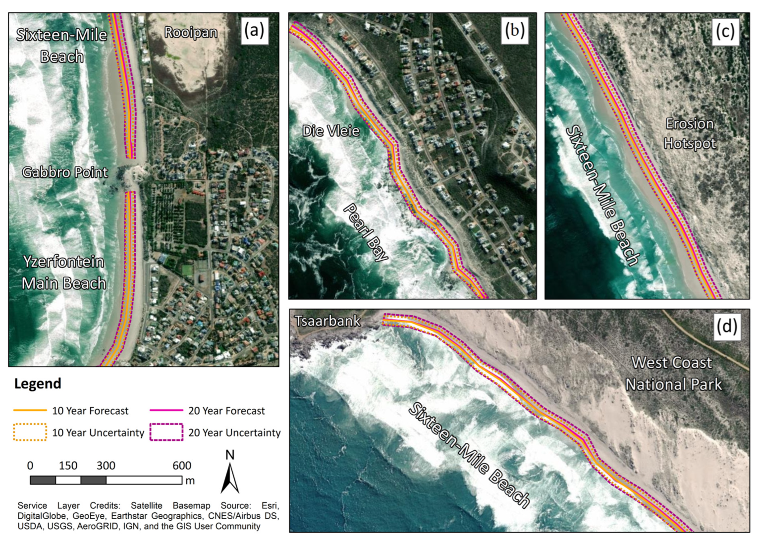
3.2. Future Shoreline Changes

In this section, we model the future shoreline position for 2030 and 2040 using the statistical trends from the long-term analysis (1937–2020) to provide a picture as to whether there are regions of concern where possible erosional trends could affect the foredune or coastal infrastructure, or if there are sections of coastline that could accrete over time. Overall, the future shoreline position modelling did not show substantial movement from the current high-water line, and the uncertainty buffers remained within the extent of the foreshore. Figure 8 illustrates four case-study examples of ~1 km stretches of coast, showing the 10-year (2030) shoreline forecast and uncertainty boundaries in orange and the 20-year (2040) in dark pink/purple.

Figure 8 shows that the two shoreline forecasts follow the general curvature of the current foreshore except for Tsaarbank (Figure 8d). The shoreline at Tsaarbank shows a series of cusps along the beach, which have been over-simplified into a straighter line by the model. The 10-year uncertainty area has an average buffer distance of 16 m (width of 32 m), and the 20-year uncertainty has an average buffer distance of 22 m (width of 44 m). These distances fall within the study site’s wide backshore and do not appear to cross the dune toe threshold—apart from along the ‘erosion hotspot’ (Figure 8c). At the ‘erosion hotspot’ (and a small Section 1 km north), the 20-year uncertainty buffer exceeds the edge of the foredune. Figure 8b shows the northern end of Pearl Bay, where the uncertainty buffer is closer to the dune toe than at Sixteen Mile Beach and Yzerfontein Main Beach (Figure 8a). However, these forecast results are limited to only the historical data provided and do not consider sediment transport processes, infrastructure or climate which impacts the coastline.

4. Discussion

Our results showed that the investigated southwest coast of South Africa underwent dynamic changes during the 83-year study period. In particular, Sixteen Mile Beach, Yzerfontein Main Beach and Pearl Bay have experienced net shoreline landward movement averaging 38 m. However, between 1937 and 2020, these beaches experienced varying degrees of erosion and accretion over eight decades. These changes were calculated by combining two different shoreline indicators that were manually and automatically extracted from aerial photographs and satellite Landsat images, respectively. Overall, Yzerfontein Main Beach was found to have experienced the least shoreline change, followed by Pearl Bay, while Sixteen Mile Beach experienced greater shoreline retreat and advance. In addition, the southern half of Sixteen Mile Beach has shown approximately 50 m of net landward shoreline movement, while the northern half has experienced less landward movement (~ 30 m) with small sections showing a seaward progradation (maximum 18.3 m).

A possible reason for these differences in erosion trends could be how the wave energy is dissipated along this extensive log-spiral beach system. For example, the rock outcrops at Pearl Bay, the harbor seawall and the Meeurots outcrop could offer these beaches more protection from the southerly wave swells. In comparison, Sixteen Mile Beach is completely exposed to wave energy and long-shore drift. However, this needs to be investigated further by a hydromorphological analysis of the sea-swell patterns to be confirmed.

The highest recorded net shoreline movement and erosion rate was found six km north of Gabbro Point and measured 99.29 m and −1.19 m/yr. Interestingly, field surveys conducted by Franceschini [45] and Franceschini and Compton [46] revealed that the beach profile and characteristics changed six km north of Gabbro Point. The average grain size changed rapidly from fine to medium between the six km and nine km mark, the calcium carbonate composition decreased, and the height of the pioneer dunes increased substantially at this point [45,46]. These studies also described this location as having an extensive backshore area (>90 m). This backshore could potentially result in CoastSat reporting greater variability in the tidal run-up, which may have affected the long-term rates of change in this study.

Moreover, the increased erosion experienced along the southern section of Sixteen Mile Beach appears to contradict Compton’s [47] theory that Dassen Island forms a ‘swell barrier’ around the southern end of Sixteen Mile Beach, allowing for sediment accumulation and transport inland to form the source of the Yzerfontein-Geelbek dune system. However, these results also confirm the findings of Franceschini and Compton [46], Kandel and Conard [48] and Henrico and Bezuidenhout [49], all noting that the Yzerfontein-Geelbek dune system has shifted northwards and decreased in size over recent decades. In addition, this study was also able to identify these trends from the historical aerial photographs, which clearly show that the dunes have receded, and the shoreline is moving landwards (Figure 9). Quantifying the dune system changes is beyond this study’s scope but could be further explored by manually digitizing these dune size changes or by object-based image classification techniques.

Additionally, our results can be compared and contrasted to Luijendijk et al. [7], who conducted a global-scale study of shoreline change by calculating erosion and accretion rates at every 500 m interval of sandy beach by extracting the shoreline positions using Landsat satellite imagery between 1984 and 2016. Their interactive web-map shows an average erosion rate of −1.71 ± 0.44 m/yr around our study site (http://shorelinemonitor.deltares.nl/, accessed on 20 December 2022).

5. Conclusions

This study analyzed the long-term shoreline changes on the southwest coast of South Africa between 1937 and 2020 and showed a net shoreline retreat, averaging 38 m landwards. Much erosion was seen along the southern stretch of Sixteen Mile Beach within the West Coast National Park. The main beach at Yzerfontein experienced the least change, followed by Pearl Bay, which experienced some erosion between 2015 and 2020.

This change could potentially be attributed to broader changes in the overall coastal and inland dune systems that have occurred over the decades or changes in regional ocean and climate systems. Regarding shoreline change rates (WLR), 47% of the shoreline showed statistically significant erosion rates and only 3% experienced rates of accretion, while the other 50% can be classified as non-significant.

Our study has reaffirmed the value of the combined use of historical aerial imagery and Landsat data, together with CoastSat, Google Earth Engine and DSAS geospatial assets, as they offer a unique opportunity to explore space-time patterns of coasts and their potential evolution in the future—notwithstanding the underlying uncertainties that follow all remotely-sensed data. On the one hand, this data integration made it possible to overcome some limitations of digitizing historical aerial photographs, which has been the standard method for studies analyzing coastal changes for over 40 years. However, this method is negatively influenced by human error and the lack of image availability. Instead, CoastSat offers a more objective, automated and advanced methodology, relying on Google Earth Engine’s extensive database of satellite imagery and machine learning capabilities.

References

1. Shetty, A.; Jayappa, K.S.; Mitra, D. Shoreline Change Analysis of Mangalore Coast and Morphometric Analysis of Netravathi-Gurupur and Mulky-Pavanje Spits. Aquat. Procedia 2015, 4, 182–189. [Google Scholar] [CrossRef]
2. Mentaschi, L.; Vousdoukas, M.I.; Pekel, J.-F.; Voukouvalas, E.; Feyen, L. Global Long-Term Observations of Coastal Erosion and Accretion. Sci. Rep. 2018, 8, 12876. [Google Scholar] [CrossRef] [Green Version]
3. Syvitski, J.; Ángel, J.R.; Saito, Y.; Overeem, I.; Vörösmarty, C.J.; Wang, H.; Olago, D. Earth’s Sediment Cycle during the Anthropocene. Nat. Rev. Earth Environ. 2022, 3, 179–196. [Google Scholar] [CrossRef]
4. Ghazali, N.H.M.; Awang, N.A.; Mahmud, M.; Mokhtar, A. Impact of Sea Level Rise and Tsunami on Coastal Areas of North-West Peninsular Malaysia. Irrig. Drain. 2018, 67, 119–129. [Google Scholar] [CrossRef]
5. Tian, H.; Xu, K.; Goes, J.I.; Liu, Q.; do Gomes, H.R.; Yang, M. Shoreline Changes along the Coast of Mainland China—Time to Pause and Reflect? ISPRS Int. J. Geo-Inf. 2020, 9, 572. [Google Scholar] [CrossRef]
6. Hinkel, J.; Nicholls, R.J.; Tol, R.S.; Wang, Z.B.; Hamilton, J.M.; Boot, G.; Vafeidis, A.T.; McFadden, L.; Ganopolski, A.; Klein, R.J. A Global Analysis of Erosion of Sandy Beaches and Sea-Level Rise: An Application of DIVA. Glob. Planet. Change 2013, 111, 150–158. [Google Scholar] [CrossRef]
7. Luijendijk, A.; Hagenaars, G.; Ranasinghe, R.; Baart, F.; Donchyts, G.; Aarninkhof, S. The State of the World’s Beaches. Sci. Rep. 2018, 8, 6641. [Google Scholar] [CrossRef] [PubMed]
8. Vousdoukas, M.I.; Ranasinghe, R.; Mentaschi, L.; Plomaritis, T.A.; Athanasiou, P.; Luijendijk, A.; Feyen, L. Sandy Coastlines under Threat of Erosion. Nat. Clim. Chang. 2020, 10, 260–263. [Google Scholar] [CrossRef]
9. Cooper, J.A.G.; Masselink, G.; Coco, G.; Short, A.D.; Castelle, B.; Rogers, K.; Anthony, E.; Green, A.N.; Kelley, J.T.; Pilkey, O.H. Sandy Beaches Can Survive Sea-Level Rise. Nat. Clim. Chang. 2020, 10, 993–995. [Google Scholar] [CrossRef]
10. Theron, A.K. Analysis of Potential Coastal Zone Climate Change Impacts and Possible Response Options in the Southern African Region. In Proceedings of the IPCC TGICA Conference: Integrating Analysis of Regional Climate Change and Response Options, Nadi, Fiji, 20–22 June 2007; pp. 205–216. Available online: https://www.ipcc.ch/site/assets/uploads/2018/08/tgica_reg-meet-fiji-2007.pdf (accessed on 10 August 2022).
11. Wigley, R. Geohazards in Coastal Areas; Council for Geoscience: Bellville, South Africa, 2011; pp. 1–12. [Google Scholar]
12. RSA South Africa’s Ocean Economy. Available online: https://www.gov.za/sites/default/files/gcis_document/201706/saoceaneconomya.pdf (accessed on 15 September 2022).
13. Fourie, J.-P.; Ansorge, I.; Backeberg, B.; Cawthra, H.C.; MacHutchon, M.R.; van Zyl, F.W. The Influence of Wave Action on Coastal Erosion along Monwabisi Beach, Cape Town. S. Afr. J. Geomat. 2015, 4, 96–109. [Google Scholar] [CrossRef]
14. Rautenbach, C.; Daniels, T.; de Vos, M.; Barnes, M.A. A Coupled Wave, Tide and Storm Surge Operational Forecasting System for South Africa: Validation and Physical Description. Nat. Hazards 2020, 103, 1407–1439. [Google Scholar] [CrossRef]
15. Barnes, M.A.; Turner, K.; Ndarana, T.; Landman, W.A. Cape Storm: A Dynamical Study of a Cut-off Low and Its Impact on South Africa. Atmos. Res. 2021, 249, 105290. [Google Scholar] [CrossRef]
16. Noujas, V.; Thomas, K.V.; Ajeesh, N.R. Shoreline Management Plan for a Protected but Eroding Coast along the Southwest Coast of India. Int. J. Sediment Res. 2017, 32, 495–505. [Google Scholar] [CrossRef]
17. Narayana, A.C. Shoreline Changes. In Encyclopedia of Estuaries; Kennish, M.J., Ed.; Springer: Dordrecht, The Netherlands, 2016; pp. 590–602. [Google Scholar]
18. Szuster, B.W.; Chen, Q.; Borger, M. A Comparison of Classification Techniques to Support Land Cover and Land Use Analysis in Tropical Coastal Zones. Appl. Geogr. 2011, 31, 525–532. [Google Scholar] [CrossRef]
19. Choung, Y.; Li, R.; Jo, M.-H. Development of a Vector-Based Method for Coastal Bluffline Mapping Using LiDAR Data and a Comparison Study in the Area of Lake Erie. Mar. Geod. 2013, 36, 285–302. [Google Scholar] [CrossRef]
20. Cabezas-Rabadán, C.; Pardo-Pascual, J.E.; Palomar-Vázquez, J.; Fernández-Sarría, A. Characterizing Beach Changes Using High-Frequency Sentinel-2 Derived Shorelines on the Valencian Coast (Spanish Mediterranean). Sci. Total Environ. 2019, 691, 216–231. [Google Scholar] [CrossRef] [PubMed]
21. Maglione, P.; Parente, C.; Vallario, A. Coastline Extraction Using High Resolution WorldView-2 Satellite Imagery. Eur. J. Remote Sens. 2014, 47, 685–699. [Google Scholar] [CrossRef]
22. Wang, X.; Liu, Y.; Ling, F.; Liu, Y.; Fang, F. Spatio-Temporal Change Detection of Ningbo Coastline Using Landsat Time-Series Images during 1976–2015. ISPRS Int. J. Geo-Inf. 2017, 6, 68. [Google Scholar] [CrossRef] [Green Version]
23. Xu, N. Detecting Coastline Change with All Available Landsat Data over 1986–2015: A Case Study for the State of Texas, USA. Atmosphere 2018, 9, 107. [Google Scholar] [CrossRef] [Green Version]
24. Specht, M.; Specht, C.; Lewicka, O.; Makar, A.; Burdziakowski, P.; Dąbrowski, P. Study on the Coastline Evolution in Sopot (2008–2018) Based on Landsat Satellite Imagery. J. Mar. Sci. Eng. 2020, 8, 464. [Google Scholar] [CrossRef]
25. Mao, Y.; Harris, D.L.; Xie, Z.; Phinn, S. Efficient Measurement of Large-Scale Decadal Shoreline Change with Increased Accuracy in Tide-Dominated Coastal Environments with Google Earth Engine. ISPRS J. Photogramm. Remote Sens. 2021, 181, 385–399. [Google Scholar] [CrossRef]
26. Liu, X.; Hu, G.; Chen, Y.; Li, X.; Xu, X.; Li, S.; Pei, F.; Wang, S. High-Resolution Multi-Temporal Mapping of Global Urban Land Using Landsat Images Based on the Google Earth Engine Platform. Remote Sens. Environ. 2018, 209, 227–239. [Google Scholar] [CrossRef]
27. Amani, M.; Brisco, B.; Afshar, M.; Mirmazloumi, S.M.; Mahdavi, S.; Mirzadeh, S.M.J.; Huang, W.; Granger, J. A Generalized Supervised Classification Scheme to Produce Provincial Wetland Inventory Maps: An Application of Google Earth Engine for Big Geo Data Processing. Big Earth Data 2019, 3, 378–394. [Google Scholar] [CrossRef]
28. Mauger, C.L.; Compton, J.S. Formation of Modern Dolomite in Hypersaline Pans of the Western Cape, South Africa. Sedimentology 2011, 58, 1678–1692. [Google Scholar] [CrossRef]
29. About Yzerfontein—Yzerfontein Tourism. Available online: https://www.yzerfonteintourism.co.za/about-yzerfontein/ (accessed on 25 September 2022).
30. Lemmen, A.C. Second Home Development in South Africa. Master’s Thesis, Utrecht University, Utrecht, The Netherlands, 2011. [Google Scholar]
31. Hanekom, N.; Randall, R.M.; Nel, P.; Kruger, N. West Coast National Park, State of Knowledge; South African National Parks Scientific Services: Sedgefield, South Africa, 2009; pp. 1–65.
32. About NGI. Available online: https://ngi.dalrrd.gov.za/index.php/home/about-ngi (accessed on 25 September 2022).
33. Fundamentals of Georeferencing a Raster Dataset—Help|ArcGIS for Desktop. Available online: https://desktop.arcgis.com/en/arcmap/10.3/manage-data/raster-and-images/fundamentals-for-georeferencing-a-raster-dataset.htm (accessed on 20 September 2020).
34. Moore, L.J.; Ruggiero, P.; List, J.H. Comparing Mean High Water and High Water Line Shorelines: Should Proxy-Datum Offsets Be Incorporated into Shoreline Change Analysis? J. Coast. Res. 2006, 22, 894–905. [Google Scholar] [CrossRef]
35. Pollard, J.A.; Brooks, S.M.; Spencer, T. Harmonising Topographic & Remotely Sensed Datasets, a Reference Dataset for Shoreline and Beach Change Analysis. Sci. Data 2019, 6, 42. [Google Scholar]
36. Hapke, C.; Schwab, W.; Gayes, P.; McCoy, C.; Viso, R.; Lentz, E. Inner Shelf Morphologic Controls on the Dynamics of the Beach and Bar System, Fire Island, New York. In Coastal Sediments 2011; Rosati, J.D., Wang, P., Roberts, T.M., Eds.; American Society of Civil Engineers: Reston, VA, USA, 2011; pp. 1034–1047. [Google Scholar]
37. Burningham, H.; Fernandez-Nunez, M. Shoreline Change Analysis. In Sandy Beach Morphodynamics; Jackson, D.W.T., Short, A.D., Eds.; Elsevier: Amsterdam, The Netherlands, 2020; pp. 439–460. [Google Scholar]
38. Niang, A.J. Monitoring Long-Term Shoreline Changes along Yanbu, Kingdom of Saudi Arabia Using Remote Sensing and GIS Techniques. J. Taibah Univ. Sci. 2020, 14, 762–776. [Google Scholar] [CrossRef]
39. Vos, K.; Splinter, K.D.; Harley, M.D.; Simmons, J.A.; Turner, I.L. CoastSat: A Google Earth Engine-Enabled Python Toolkit to Extract Shorelines from Publicly Available Satellite Imagery. Environ. Model. Softw. 2019, 122, 104528. [Google Scholar] [CrossRef]
40. McFeeters, S.K. The Use of the Normalized Difference Water Index (NDWI) in the Delineation of Open Water Features. Int. J. Remote Sens. 1996, 17, 1425–1432. [Google Scholar] [CrossRef]
41. Vos, K.; Harley, M.D.; Splinter, K.D.; Simmons, J.A.; Turner, I.L. Sub-Annual to Multi-Decadal Shoreline Variability from Publicly Available Satellite Imagery. Coast. Eng. 2019, 150, 160–174. [Google Scholar] [CrossRef]
42. Himmelstoss, E.A.; Henderson, R.E.; Kratzmann, M.G.; Farris, A.S. Digital Shoreline Analysis System (DSAS) Version 5.0 User Guide; Open-File Report 2018–1179; US Geological Survey: Reston, VA, USA, 2018.
43. Burningham, H.; French, J. Understanding Coastal Change Using Shoreline Trend Analysis Supported by Cluster-Based Segmentation. Geomorphology 2017, 282, 131–149. [Google Scholar] [CrossRef]
44. Sarkar, D.; Andrews, F.; Wright, K.; Klepeis, N.; Murrell, P. Lattice: Trellis Graphics for R 2021. Available online: https://cran.r-project.org/web/packages/lattice/index.html (accessed on 21 August 2022).
45. Franceschini, G. Geology of Aeolian and Marine Deposits in the Saldanha Bay Region, Western Cape, South Africa. Ph.D. Thesis, University of Cape Town, Cape Town, South Africa, 2003. [Google Scholar]
46. Franceschini, G.; Compton, J.S. Holocene Evolution of the Sixteen Mile Beach Complex, Western Cape, South Africa. J. Coast. Res. 2006, 22, 1158–1166. [Google Scholar] [CrossRef] [Green Version]
47. Compton, J. The Rocks and Mountains of Cape Town; Earthspun Books: Cape Town, South Africa, 2019; pp. 73–105. [Google Scholar]
48. Kandel, A.W.; Conard, N.J. Stone Age Economics and Land Use in the Geelbek Dunes. In The Archaeology of the West Coast of South Africa; Archaeopress: Oxford, UK, 2013; pp. 24–49. [Google Scholar]
49. Henrico, I.; Bezuidenhout, J. Determining the Change in the Bathymetry of Saldanha Bay Due to the Harbour Construction in the Seventies. S. Afr. J. Geomat. 2020, 9, 236–249. [Google Scholar] [CrossRef]
Figure 1. Overview of satellite imagery over the study area showing three coastal areas studied (a); Sixteen Mile Beach, Yzerfontein Main Beach and Pearl Bay (b); and the location of the study sites in the Western Cape Province of South Africa (c).
Remotesensing 15 00317 g001
Figure 2. Flowchart of the overall methodology for assessing the shoreline changes.
Remotesensing 15 00317 g002
Figure 3. (a) Map of a perpendicular transect through the shoreline positions from the different time periods and their respective uncertainty values as buffers. (b) Plot of the linear regression and weighted linear regression for distance from the baseline versus time.
Remotesensing 15 00317 g003
Figure 4. (a) Map of net shoreline movement (NSM) along the study site with warm colors representing erosion and cool colors representing accretion. (b) Graph of NSM vs. 100 m-transects along the coast.
Remotesensing 15 00317 g004
Figure 5. (a) Map of the Weighted Linear Regression rates along the study site with warm colors representing erosion and cool colors representing accretion. (b) Graph of WLR at every 100 m transect along the coast and the 95% confidence interval.
Remotesensing 15 00317 g005
Figure 6. Summary of DSAS results showing (a) the Net Shoreline Movement (NSM), (b) Shoreline Change Envelope (SCE), (c) End Point Rate (EPR), (d) Linear Regression Rate (LRR), and (e) the Weighted Linear Regression (WLR).
Remotesensing 15 00317 g006
Figure 7. Time series heat-matrix represents the amount of change to the shoreline regarding the 1937 shoreline position over the eleven time periods.
Remotesensing 15 00317 g007
Figure 8. Shoreline position forecasts for the next 10 and 20 years with their horizontal uncertainty for four locations along the study site: (a) Yzerfontein Main Beach and the southern end of Sixteen Mile, (b) the northern end of Pearl Bay, (c) the erosion hotspot located 6 km north of Gabbro Point, and (d) the northern end of Sixteen Mile Beach at Tsaarbank.
Remotesensing 15 00317 g008
Figure 9. A comparison between (a) the historical aerial photograph from 1937 and (b) the panchromatic Landsat-8 image from 2020 showing the change in shoreline position and coastal dune distribution.
Remotesensing 15 00317 g009