Abstract
Hyperspectral Image (HSI) classification methods that use Deep Learning (DL) have proven to be effective in recent years. In particular, Convolutional Neural Networks (CNNs) have demonstrated extremely powerful performance in such tasks. However, the lack of training samples is one of the main contributors to low classification performance. Traditional CNN-based techniques under-utilize the inter-band correlations of HSI because they primarily use 2D-CNNs for feature extraction. Contrariwise, 3D-CNNs extract both spectral and spatial information using the same operation. While this overcomes the limitation of 2D-CNNs, it may lead to insufficient extraction of features. In order to overcome this issue, we propose an HSI classification approach named Tri-CNN which is based on a multi-scale 3D-CNN and three-branch feature fusion. We first extract HSI features using 3D-CNN at various scales. The three different features are then flattened and concatenated. To obtain the classification results, the fused features then traverse a number of fully connected layers and eventually a softmax layer. Experimental results are conducted on three datasets, Pavia University (PU), Salinas scene (SA) and GulfPort (GP) datasets, respectively. Classification results indicate that our proposed methodology shows remarkable performance in terms of the Overall Accuracy (OA), Average Accuracy (AA), and Kappa metrics when compared against existing methods.
1. Introduction
Hyperspectral Imaging (HSI) systems collect spectral and spatial image data simultaneously in hundreds of narrow contiguous spectral bands, from visible to infrared wavelengths. Applications for HSI remote sensing are numerous, such as environmental monitoring [1,2], agriculture [3,4,5,6], mineralogy [7,8,9], and surveillance [10,11,12]. Each pixel in the image consists of hundreds of elements measuring the reflected or emitted energy as a function of wavelength, known as the spectral response. Unlike common or normal images, hyperspectral ones carry information about the material’s chemical and physical properties since the interaction of a substance with light depends on its atomic and molecular structure, HSIs are rich in spectral information that reflect the material’s chemical and physical properties, which makes image classification tasks easier.
HSI classification has become one of the most active research topics in the field of HSI analysis [13,14] and has drawn the attention of researchers in the remote sensing field. It is defined as the task of assigning each pixel of the HSI to one certain class based on its spectral characteristics. There are challenges faced in most of the HSI classification tasks due to high-dimensional characteristics of HSI data and the similarity of spectra and mixed pixels. The following challenges need to be addressed:
- The lack of ground-truth data or labeled samples: A typical challenge in remote sensing is that images are acquired from a far distance, which makes it difficult to distinguish the materials by the a simple observation. In many applications, scientists need to go to the field of study to observe the materials in the scene from a close distance.
- HSIs have high dimensionality: This is related to the large number of channels (or bands) that HSI has. As the number grows, the data distribution becomes sparse and hard to model, which is also known as the curse of dimensionality problem, a term that was introduced by Bellman et al. [15]. However, multiple adjacent bands are similar and present redundant information, which enables the ability to use dimensionality reduction techniques to reduce the amount of involved data and speed up the classification process.
- Low spatial quality: Sensors suffer from a trade-off that allows capturing images either with high spatial resolution or high spectral resolution. Thus, HSIs generally have relatively low spatial resolution when compared to natural images.
- Spectral variability: The spectral response of each observed material can be significantly affected by atmospheric variations, illumination, or environmental conditions.
Machine Learning (ML) techniques were first used in the early research studies of HSI classification. These techniques use pixel-wise classification methods to classify each pixel in HSI data based on spectral information. Support Vector Machine (SVM) [16], Multinomial Logistic Regression (MLR) [17], Random Forest (RF) [18], and K-Nearest Neighbor (KNN) [19] are the most common examples of traditional approaches. However, these methods ignore the spatial information and rely solely on the spectral information of the pixels, which affects the classification performance. In order to tackle this challenge, Deep Learning (DL) techniques were utilized to obtain the spatial features along with the spectral ones. The DL approaches used for HSI classification are mainly Convolutional Neural Networks (CNNs), Autoencoders [20], Deep Belief Networks [21], Generative Adversarial Networks (GANs) [22,23], and Recurrent Neural Networks (RNNs) [24,25].
Related Work
As previously mentioned, the high-dimensionality characteristic of HSI data makes HSI classification a challenging task. Therefore, dimensionality reduction is a necessary pre-processing step prior to the classification task in order to reduce the redundancy and complexity of data. Numerous studies have been conducted to find a solution to the HSI’s curse of dimensionality problem. So far, these dimensionality reduction techniques can be grouped into two main categories; feature extraction and band selection. Feature extraction approaches can be divided further into two groups; supervised and unsupervised feature extraction. Supervised feature extraction approaches utilize label information to maximize between-class separation, such as Linear Discriminant Analysis (LDA) [26], and Fisher’s Linear Discriminant Analysis (FLDA) [27]. As for unsupervised feature extraction methods, they include Principal Component Analysis (PCA) [28,29] and Kernel PCA (KPCA) [30,31] that extract useful linear and nonlinear features, respectively, from HSI data. As for band selection dimensionality reduction, it is implemented by selecting the most descriptive and distinctive band subset from the original band space of the HSIs according to certain criteria or search strategy. Band selection approaches can be categorized into supervised, semi-supervised and unsupervised.
In recent years, DL methods, specifically, Convolutional Neural Networks (CNNs), have received an increased attention and have been widely employed in various computer vision tasks. CNNs can learn and extract deep features from raw data through a sequence of hierarchical layers; shallower layers can extract edges and texture features, whilst the deeper layers extract more complex features. Thus, CNNs have been extended and introduced for HSI classification [32]. The authors in [33] utilized PCA as pre-processing technique to handle data dimensionality. Then, the reduced components were fed to three consecutive 2D convolutional layers for feature mapping, followed by a flattening layer to convert all 2D feature maps into 1D feature vectors, which were then passed to fully connected layers to perform the final classification of the HSI. Similarly, in [34], the authors presented a CNN approach based on information measure and enhanced spectral information where both spectral and spatial information are measured and used as an input to the CNN classifier. Dimensionality reduction is also employed using entropy calculation in order to select the three most informative spectra from HSI bands. Accurate classification of HSI was achieved under the reduced computational complexity.
In another study [35], Li et al. proposed a two-stream spectral and spatial feature extraction and fusion network based on Two-dimensional CNN (2D-CNN) architecture. The purpose of using the two extraction networks, shallow and deep, with different depth is to obtain multi-scale spectral, local, and global spatial information. Furthermore, an attention mechanism based on Squeeze and Excitation (SE) networks was adopted in this study to improve the capability of extracting useful spectral–spatial features and to overcome the lack of labeled training data. In addition to 2D-CNNs, Three-dimensional Convolutional Neural Networks (3D-CNNs) have been extensively studied for HSI classification as well. The authors in [36] presented a novel 3D-CNN approach for HSI classification, in which both spectral and spatial information are utilized to boost the classification performance. In a similar approach, the researchers in [37] introduced a 3D-CNN model for HSI classification, the HSI is first split into small overlapping 3D patches, which are then processed to create 3D feature maps utilizing a 3D kernel function over multiple contiguous bands of the spectral information in an effective manner. Since then, there has been an increasing number of HSI studies based on 2D-CNN or 3D-CNN [38,39,40].
However, there are a few drawbacks to utilizing either 2D-CNN or 3D-CNN for HSI classification. In the case of 2D-CNN architectures, even though they excel at obtaining spatial information, they fall short with regards to extracting good discriminating or informative feature maps from the spectral dimensions. On the other hand, 3D-CNNs are considered computationally expensive as a large number of 3D convolution operations are invoked. Deep 3D-CNNs require more training samples, which is not possible due to the limited dataset size provided by the publicly available HSI datasets. Furthermore, most of the common 3D-CNN-based approaches consist of stacked 3D convolutions within their architecture. Hence, they cannot optimize the estimation loss directly through such a nonlinear structure [41].
In order to tackle these limitations, many authors have introduced a hybrid approach. For example, in [42], the authors introduced a hybrid model called HybridSN, which fuses 2D-CNN with 3D-CNN to effectively extract both spectral and spatial feature maps from HSI. This improves the accuracy of the classification results. Similarly, in [43], the authors used 2D- and 3D-CNNs to extract spatial and spectral features in HSI, respectively. An attention mechanism is also utilized to combine these two kinds of features. In another study [44], the researchers presented a 3D fast learning block followed by 2D convolution for HSI data. The 3D block consists of 3D depthwise separable convolution and fast convolution blocks. The proposed approach shows superior performance in terms of training time and learning parameters when compared to existing 2D-CNN and 3D-CNN architectures. In another study [41], a hybrid model, named Synergistic CNN (SyCNN) is proposed. The model also combines 2D and 3D convolution to extract the spectral and spatial information in turn. Moreover, the least important features are removed by introducing a 3D attention mechanism before the fully-connected layer. To tackle the issue of a limited number of labeled samples, Zhang et al. [45] proposed a 3D lightweight CNN model by introducing two different transfer learning strategies; cross-sensor strategy and cross-modal strategy. The first strategy transfers models between HSI datasets captured by the same or different sensor, whereas the second one uses a pre-trained 3D-CNN model on 2D RGB, or natural, image data sets to train 3D HSI through fine tuning the model. The proposed approach also reduces the number of trainable parameters while improving the classification’s accuracy. Xu et al. [46] introduced a robust self-ensembling network (RSEN) that consists of two subnetworks; base network and an ensemble network. Experiments show good performance with very limited labeled training samples when compared to state-of-the-art methods. Although the CNN-based approaches have proven their efficiency in HSI classification task, they still encounter a series of challenges such as, the receptive field is limited, information is lost in down-sampling layer, and a lot of computing resources are consumed for training deep networks. To overcome this challenge, transformer-based network is used to replace the traditional CNN to perform HSI classification tasks. The authors in [47] introduced a multilevel spectral–spatial transformer network (MSTNet) for hyperspectral classification. The proposed model incorporates an image-based classification framework for HSI in order to extract richer global information. Experimental results show that the proposed approach outperforms other CNN-based methods for classification.
Many researchers employ a multi-scale approach. It is an effective way for improving the classification accuracy due to the different sizes of land covers, which can capture more important information [48]. The spatial spectral unified network (SSUN) proposed in [49] utilizes this strategy. This approach combines the long short-term memory (LSTM) model as the spectral feature extractor with 2D-CNN for extracting spatial features and integrating the spectral Finite Element (FE), spatial FE, and classifier training into one unified network. By extracting multi-scale spectral–spatial features simultaneously (since diverse layers in CNN will produce different scale features) the Multi-Scale Convolutional Neural Network (MSCNN) [49] encompasses multi-scale characteristics. The experiments showed that the full use of both spectral and spatial information can considerably boost the classification accuracy. Although the existing spectral–spatial based methods show excellent performance in HSI classification but most of them are focusing on processing the pixels adjacent to the central pixels and neglect the implicit spatial information between features which in turn affects the performance of the classification model. To tackle this problem, Parallel Multi-Input Mechanism CNN (PMI-CNN) is introduced by Zhong et al. [50]. This model employs a parallel multi-input approach by using four parallel convolution branches to extract spatial features with different levels or window sizes in HSI data. Each branch of the network adopts four different convolution kernels to carry out multi-scale convolution on the inputs, of which convolution kernel is used to extract spectral features of HSIs that will be fused with spatial information to classify HSI data. Their approach shows superiority in terms of overall accuracy and kappa metrics.
The following is a list of this paper’s main contributions:
- A new model that incorporates feature extraction at different filter scales is proposed, which effectively improves the classification performance.
- A deep feature-learning network based on various dimensions with varied kernel sizes is created so that the filters may concurrently capture spectral, spatial, and spectral–spatial properties in order to more effectively use the spatial-spectral information in HSIs. The proposed model has a better ability to learn new features than other models that are already in use, according to experimental results.
- The proposed model not only outperforms existing methods in the case of smaller number of samples, but also achieves better accuracy with enough training samples, according to statistical results from detailed trials on three HSIs that will be reported and discussed in the next sections.
- The impact of different percentages of training data on model performance in terms of OA, AA and kappa metrics are also examined.
2. Methodology
2.1. Framework of the Proposed Model
The methodology consists of two parts; data pre-processing and the proposed CNN. The details of these parts are explained in the next subsections.
2.1.1. Data Preprocessing
As stated in Section 1, HSI data must be pre-processed to reduce their dimensionality before processing them with DLmodels. In this research, PCA [28] is used to fulfill this role. PCA is one of the widely used unsupervised techniques for dimensionality reduction and feature extraction. It is based on the fact that adjacent bands of HSI exhibit strong correlation and frequently represent the same information about the object. It is carried out using an orthogonal transformation, which considers a set of variables that could be correlated and transforms or projects them into a set of values that are linearly uncorrelated and are known as Principal Components (PCs). Assuming the size of raw HSI cube is , where H and W are the height and width of the HSI, respectively, and C is the depth (number of spectral bands). PCA works by downsizing the raw HSI cube’s depth from C to D in such a way that the reduced HSI cube will be of size , where D is the new spectral dimension and .
2.1.2. Architecture of the Proposed Tri-CNN
Currently, the majority of the models use 2D-CNN or 3D-CNN architectures for HSI classification tasks. 2D-CNN has the ability to capture the spatial information; however, it ignores the rich spectral information provided by the HSI. On the other hand, 3D-CNN can extract both spectral and spatial information simultaneously, which may lead to insufficient extraction of features. In order to solve these shortcomings, the spatial feature extractor and the spectral–spatial feature extractor are combined along with spectral-only feature extractor to form a three-branch feature fusion network. The purpose of adding this path to the architecture is to enhance the extraction of spectral feature characteristics and improve the overall feature extraction process.
It is worth mentioned that the spatial feature extractor was designed with multiple 3D convolution filters. A number of smaller convolution kernels can extract features more effectively with lower computational cost [51], when compared to large convolution kernels. To extract the spectral features, multiple 3D convolution filters were used. Using a convolution kernel with of this size makes the model only focus on a specific pixel when extracting the spectral features, This can deal with the problem of adding unrelated information and improve the model’s classification performance.
The flattening layer is used to convert each feature extracted by each branch into a one-dimensional vector. Then, all vectors are fused to produce the final classification results. This is achieved by concatenating the three one-dimensional features into a new one-dimensional vector, whose dimension number equals the total of the three feature dimensions. The flattened features at each branch are of different length (as shown in Section 3.3, adding them directly is not possible. Hence, concatenation was the most suitable choice for feature fusion.
The detailed distribution and parameters of each layer in the proposed approach are shown in Figure 1. The first branch has 2 layers of 3D-CNN with 64 filters and the kernel size is set to to capture spectral features. The second branch captures the spatial features by setting the kernel size to with the same number of layers and filters in the first branch. While the third branch is designed to capture both spectral and spatial features simultaneously by having 3D-CNN layers and using 64 filters and setting the kernel size of each filter to . Due to the fact that the pooling layer causes loss of information, it has not been used within the network architecture. In addition, the network structure and hyperparameters described above perform well on all HSI datasets used in this research.
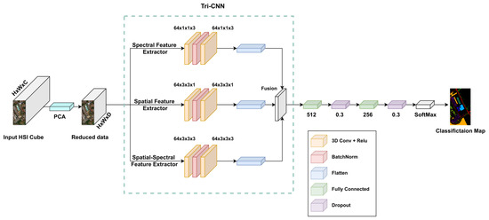
Figure 1.
Framework of the proposed model.
2.2. Loss Function
Cross-Entropy (CE) is used as the loss function in this paper. The formula is given by:
where and are the reference and predicted labels, respectively, M and L are the overall number of small batch samples and land cover categories, respectively.
3. Experiments and Analysis
In this section, we will present details of the HSI datasets used in this paper. Secondly, we will introduce the the experimental configuration and parameter analysis. Then, we will apply the ablation experiments on the proposed model. Finally, we will perform a comparison between the proposed model against existing methods to prove the model superiority and its effectiveness both quantitatively and qualitatively.
3.1. Datasets
In our experiments, two of the most commonly used HSI datasets are adopted, namely, Pavia University and Salinas. Additionally, the Gulfport of Mississippi dataset is also used as well, although that it has not been widely used for HSI classification tasks, it is of great interest as it is small in size and consists of 72 spectral bands only. Each of these dataset has its own specifications, which are listed as follows:
- Pavia University (PU): This is a scene acquired with the Reflective Optics Imaging Spectrometer Sensor (ROSIS) during a flight campaign over Pavia, northern Italy. The image consists of 103 spectral bands with wavelengths ranging from 0.43 to 0.86 m and a spatial resolution of 1.3 m. The size of Pavia University is pixels. Figure 2a shows RGB color composite of the scene. The reference classification map in Figure 2b shows nine classes, with the unassigned pixels colored in black and labeled as Unassigned. Table 1 shows the number of pixels per each class in the data set.
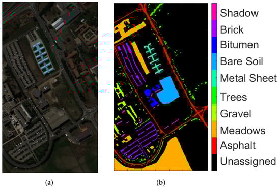 Figure 2. ROSIS Pavia University (a) true-color composite; (b) reference class map.
 Table 1. Groundtruth classes for PU scene and their respective samples number.
 - Salinas (SA): This scene was collected by the Airborne Visible/Infrared Imaging Spectrometer (AVIRIS) sensor over Salinas Valley, California. The image consists of 224 spectral bands with wavelengths ranging from 0.4 to 2.45 m and a spatial resolution of 3.7 m. The size of Salinas is pixels. Bands 108–112, 154–167, and 224 were removed due to distortions from water absorption. Figure 3a shows RGB composite of the scene. The reference classification map in Figure 3b shows that Salinas ground truth class map contains 16 classes. Similar to PU, unassigned pixels are colored in black and labeled as Unassigned. Table 2 shows number of pixels per class in the data set.
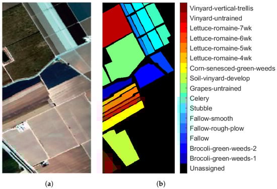 Figure 3. AVIRIS Salinas (a) true-color composite; (b) reference class map.
Table 2. Groundtruth classes for SA scene and their respective samples number.
Figure 3. AVIRIS Salinas (a) true-color composite; (b) reference class map.
Table 2. Groundtruth classes for SA scene and their respective samples number. - Mississippi Gulfport (GP): The dataset was collected over the University of Southern Mississippi’s-Gulfpark Campus [52]. The image consists of 72 bands with wavelengths ranging from 0.37 to 1.04 m and a spatial resolution of 1.0 m. The size of GP is pixels. Figure 4a shows RGB color composite of the scene. The reference classification map in Figure 4b shows six classes. As with PU and SA datasets, the unassigned pixels in the image are colored in black and labeled as Unassigned. Table 3 shows the number of pixels per class in the dataset.
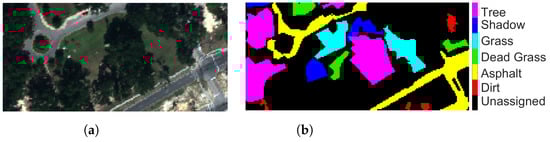 Figure 4. Mississippi Gulfport (a) true-color composite; (b) reference class map.
Table 3. Groundtruth classes for Gulfport of Mississippi scene and their respective samples number.
Figure 4. Mississippi Gulfport (a) true-color composite; (b) reference class map.
Table 3. Groundtruth classes for Gulfport of Mississippi scene and their respective samples number.
3.2. Evaluation Metrics
To evaluate the performance of classification results, predicted class maps are compared with the available reference or ground truth data. Verifying the correctness of pixel assignment in the image with visual inspection is subjective and might not be comprehensive. Therefore, quantitative evaluation is more reliable. The most common example is the Overall Accuracy (OA), which computes the number of correctly assigned HSI pixels over the number of overall samples, and it is expressed as Equation (2):
Average Accuracy (AA) [53] is another evaluation criteria used to assess the classification performance. It estimates the mean of the classification accuracy of all categories or classes. It is defined as Equation (3):
where c is the number of classes, and x is the percentage of correctly assigned pixels in a single class. Additionally, Kappa coefficient (k) [54] is also adopted to evaluate the quality of the classification results of HSI data. It is expressed as Equation (4):
where, k determines the agreement between the predicted classified map and the ground truth, and represents the expected agreement between the model classification map and the ground truth map by chance probability. Kappa values range between 0 and 1, such that 1 shows complete agreement between the predicted output and the ground truth, and vice versa for 0. Usually, Kappa ≥ 0.80 indicates a substantial agreement, while k < 0.4 indicates poor model performance.
3.3. Experimental Configuration
All the experiments have been operated using the compiler and deep learning frameworks; Python 3.8 and TensorFlow 2.4.0, respectively. Adam is adopted as the optimizer algorithm, where the learning rate is , the batch size is 16 and the training epoch is set to 100. The network configuration of the proposed model using PU dataset is shown in Table 4. The number of samples used for training the model is set to for all three datasets to guarantee a fair comparison.
Table 4.
The network configuration for the proposed model on the Pavia University dataset.
3.4. Experimental Results
In this section, classification performance of the proposed model is evaluated quantitatively and qualitatively using the three aforementioned datasets: Pavia University (PU), Salinas (SA) and Mississippi Gulfport (GP). Furthermore, the proposed methodology is compared with six state-of-the art algorithms. In order to reduce the fluctuation of classification results caused by the randomness of sample selection, the experiments were repeated 10 times, and the average value of these experiments is used as the final result. Additionally, classification results for each category are reported.
3.4.1. Analysis of Parameters
In this section, we examine how the spatial dimension and number of principal components of different datasets affect the proposed model’s ability to classify the HSI data and determine the window size and spectral dimension that are best suited for the dataset.
The window size indicates how much of the retrieved 3D patch’s spatial information can be used to assign a label to the HSI patch. A large window may include a lot of neighborhood data that may contain information from other classes, which hinders the feature extraction process. On the contrary, if the chosen window is too small, the model’s ability to extract features will suffer from a significant loss of spatial information. This research validates the impact of window size on model performance over the three aforementioned datasets. In the experiment, the spatial size was set to {, , , , , , }, while the spectral dimension was uniformly set to 30. It is clear from Figure 5 that for the PU, SA and GP datasets, the suitable window size for the proposed model was , and , respectively. As seen from the Figure, the overall accuracy for the GP dataset varies in a notable manner with respect to the window size. Since the model was trained with only 1% of the data (60 training samples), we assume that any small change in the initial settings may lead to a large impact on the model performance.
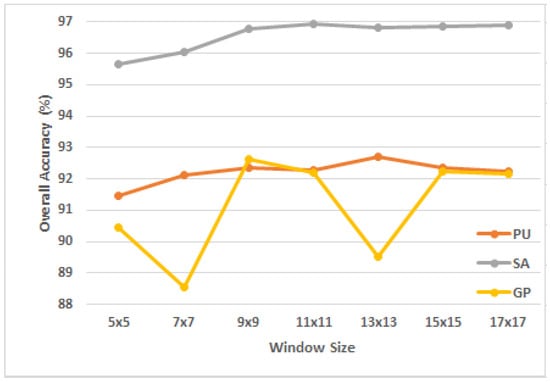
Figure 5.
The OA of the proposed model using different values of window size in the three datasets.
Moreover, the spectral dimension (or number of principal components) shows how much of the 3D patch’s collected spectral data can be used to assign a label to the HSI patch. It is intuitive that the model performance increases with the increase of the spectral dimension. However, having many principal components may contain redundant information, which causes the OA to fall after a certain value. This paper validates the impact of spectral dimension on model performance on the three datasets. In the experiment, the spectral dimension was set to 10, 15, 20, 25, 30, 35, 40, 45, 50, and the spatial size of the three datasets of PU, SA and GP were set to , , , respectively. As can be seen from Figure 6, for PU, SA and GP datasets, the most suitable spectral dimensions for the proposed model were 15, 35, and 45, respectively.
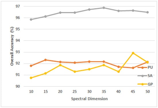
Figure 6.
The OA of the proposed model using different spectral dimension in the three datasets.
Based on the above parameter analysis, Table 5 summarizes the optimal values of window size and spectral dimension for the proposed model.
Table 5.
The optimal window size and spectral dimension of the proposed model on three HSI datasets.
3.4.2. Ablation Studies
To fully demonstrate the effectiveness of the proposed model, the influence of different combinations of the model components that belong to the network on the GP dataset is investigated and reported in Table 6. The results show that our proposed fusion technique obtains the best performance compared with other combination or fusion approaches such as spectral, spatial, spectral–spatial, spectral+spatial, spectral+spectral–spatial, and spatial+spectral–spatial in terms of AA, OA, and Kappa metrics.
Table 6.
Results of ablation studies on different combination of model branches over the GP dataset.
3.4.3. Comparison with Other Methods
For the sake of validating the proposed classification algorithm, SVM [16], 2D-CNN [55], 3D-CNN [56], PMI-CNN [50], HybridSN [42], and MSCNN [49] are used as comparison algorithms. As mentioned earlier, the experiments were conducted and repeated 10 times. For all algorithms, only the classification results with the highest accuracy in 10 trials are recorded. The quantitative comparisons of these compared methods are shown in Table 7, Table 8 and Table 9, and the best results in each Table are shown in bold.
Table 7.
Classification results on the PU dataset with 1% labeled training samples. The best accuracy is shown in bold.
Table 8.
Classification results on the SA dataset with 1% labeled training samples. The best accuracy is shown in bold.
Table 9.
Classification results on the GP data set with 1% labeled training samples. The best accuracy is shown in bold.
From Table 7, Table 8 and Table 9, we conclude that the proposed Tri-CNN model outperforms other methods. Among the datasets used in this paper, PU has 42776 labeled samples of which 1% (428 samples) was used for training the model, it has only 9 classes, which makes it easier to classify. SA has a large number of labeled samples where 542 of them where used for training, so it is no surprising that the classification performance on SA is higher. GP is relatively small dataset where it has only 6079 labeled samples, which results in lower classification accuracy since the training has been conducted with only 1% of the labeled samples.
On the PU dataset, SVM method had the lowest overall accuracy, since it utilizes only spectral information. 2D-CNN further improved the accuracy by almost 6% when compared to SVM, 2D-CNN that uses 2D filters to extract spatial information for classification. 3D-CNN had higher accuracy with 92.13%, it uses 3D filters to extract spatial and spectral information simultaneously to further improve classification accuracy. PMI-CNN extracts spatial features by using four parallel branches of two dimensional kernels, extracted features are then fused and used as the input of the classifier; however, it did not show any improvement over 3D-CNN and the accuracy was less by 1.73%. HybridSN uses 3 layers of 3D-CNN followed by one layer of 2D-CNN to extract both spectral–spatial (3D-CNN) and spatial (2D-CNN), it had higher accuracy when compared to the aforementioned models. The multi-scale CNN (MSCNN) Fuses the spatial features of different scales by using multiple two dimensional kernels to classify HSIs. Our proposed method was approximately 0.32% higher than HybridSN in terms of overall accuracy and outperformed other methods in 5 categories. The results of comparison are shown in Table 7. To have a visual comparison of the results, Figure 7 shows the classification results of the seven methods along with the reference map. It is clearly observed from Figure 7a that the results of SVM has a large number of incorrectly assigned pixels and the classification accuracy is low. The classification map of our proposed Tri-CNN method was the closest to the reference map, specially at the area bounded with the white box.
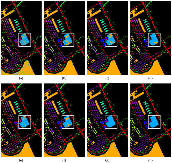
Figure 7.
Classification maps for PU dataset. (a) SVM; (b) 2D-CNN; (c) 3D-CNN; (d) HybridSN; (e) PMI-CNN; (f) MSCNN; (g) Proposed method (h) Reference map.
Table 8 shows the results of SA dataset. Our proposed method was the highest in terms of OA, AA and Kappa. The model had the highest accuracy in nine out of the sixteen classes, three of which reached 100% accuracy. Figure 8 shows the classification maps of the methods used in this research along with the reference map. The classification maps of our method are closest to the ground-truth map. The area in the white box (Class #8) shows the part that easily distinguished, which matches the results shown in Table 8.
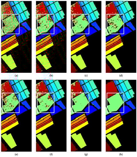
Figure 8.
Classification maps for Salinas SA. (a) SVM; (b) 2D-CNN; (c) 3D-CNN; (d) HybridSN; (e) PMI-CNN; (f) MSCNN; (g) Proposed method; (h) Reference map.
The classification results of GP dataset are shown in Table 9. Our proposed method was the highest in terms of OA, AA and Kappa when compared to the other methods. The model had the highest accuracy in three classes. Figure 9 shows the classification results of the methods used in this research. it is very clear that our proposed methods has the closest classification map to the reference data, specially the area in the white box (Class #1). This particular class had only 2 samples for training, and yet, our model had achieved a classification score of 86.85%, which is extremely higher than the second best (3D-CNN) where the score was only 16%. A similar result is shown in Class #3 (labeled in Green color), where the training was conducted with only 4 samples. This shows the ability of our model to be trained on very small datasets and still good results.
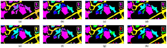
Figure 9.
Class maps of GP. (a) SVM; (b) 2D-CNN; (c) 3D-CNN; (d) HybridSN; (e) PMI-CNN; (f) MSCNN; (g) Proposed method; (h) Reference map.
Based on the experimental results, the proposed Tri-CNN produces better results when compared to the other classification methods used in this research. SVM has the worst classification performance since it utilizes spectral features only and loses the spatial information. 2D-CNN, PMI-CNN and MSCNN take into account the spatial information and the overall accuracy was improved when compared to SVM. 3D-CNN extracts spectral and spatial features simultaneously from the 3 dimensional image patch, which preserves the features in the data given. HybridSN combines both 2D-CNN and 3D-CNN to extract the spectral and spatial features to perform the image classification. Our proposed Tri-CNN method produced the best results when applied to the three datasets used in this research. Our model combines the advantage of each branch to extract features at each scale to improve the classification performance.
3.4.4. Performance of Different Models at Different Percentages of Training Data
The performance of the model can be well inferred from the classification accuracy under various percentages of training data. We randomly select 1%, 2%, 3%, 4% and 5% of labeled samples for training and the remaining was used for testing. Classification results of each dataset are shown in Figure 10. It is seen that for all the methods used in this study, classification accuracy improves as the number of training samples increases. The proposed model, which performs the best on all training sample proportions on the three datasets, uses 3D-CNN with various kernel sizes to extract various degrees of features from the HSI.
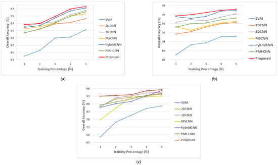
Figure 10.
Classification accuracy at different percentages of training data (a) PU; (b) SA; (c) GP.
4. Conclusions
In this paper, we propose a new three-branch CNN model namely Tri-CNN for HSI classification. The proposed model builds a three-branch feature fusion structure and optimizes the creation of the CNN-based model in order to address the current issues with HSI classification. The model feeds the data into three branches of multiscale 3D-CNN after PCA, features generated of each branch are then flattened and fused, fully connected and dropout layers are utilized to produce the final classification result. Experimental results indicate that the proposed model performs well in terms of OA, AA, and Kappa. With just a little amount of training data, the model produces nearly identical classification results.
For future work, we will examine the use of a lighter architecture with less training parameters to reduce the computational complexity without weakening the model performance. In addition, the classification accuracy of the GP dataset was relatively lower compared to other two datasets. Therefore, the focus of our future study will be on investigating a more compact neural network model, broadening the generalization ability, and achieving adequate classification accuracy on different datasets.
Author Contributions
Conceptualization, M.Q.A., M.A.-S. and N.A.; Formal analysis, M.Q.A.; Funding acquisition, S.A. and H.A.-A.; Methodology, M.Q.A. and M.A.-S.; Project administration, S.A. and H.A.-A.; Software, M.Q.A.; Supervision, M.Q.A. and H.A.-A.; Validation, M.Q.A. and N.A.; Writing—original draft, M.Q.A. and M.A.-S.; Writing—review & editing, N.A., J.Z. and S.M. All authors have read and agreed to the published version of the manuscript.
Funding
This research received no external funding.
Data Availability Statement
The PU and SA datasets can be obtained from: www.ehu.eus/ccwintco/index.php?title=Hyperspectral_Remote_Sensing_Scenes (accessed on 28 November 2022). The GP dataset can be obtained from: https://github.com/GatorSense/MUUFLGulfport (accessed on 28 November 2022).
Conflicts of Interest
The authors declare no conflict of interest.
References
- Moroni, M.; Lupo, E.; Marra, E.; Cenedese, A. Hyperspectral image analysis in environmental monitoring: Setup of a new tunable filter platform. Procedia Environ. Sci. 2013, 19, 885–894. [Google Scholar] [CrossRef]
- Stuart, M.B.; McGonigle, A.J.; Willmott, J.R. Hyperspectral imaging in environmental monitoring: A review of recent developments and technological advances in compact field deployable systems. Sensors 2019, 19, 3071. [Google Scholar] [CrossRef] [PubMed]
- Ad ao, T.; Hruška, J.; Pádua, L.; Bessa, J.; Peres, E.; Morais, R.; Sousa, J.J. Hyperspectral imaging: A review on UAV-based sensors, data processing and applications for agriculture and forestry. Remote Sens. 2017, 9, 1110. [Google Scholar] [CrossRef]
- Dale, L.M.; Thewis, A.; Boudry, C.; Rotar, I.; Dardenne, P.; Baeten, V.; Pierna, J.A.F. Hyperspectral imaging applications in agriculture and agro-food product quality and safety control: A review. Appl. Spectrosc. Rev. 2013, 48, 142–159. [Google Scholar] [CrossRef]
- Park, B.; Lu, R. Hyperspectral Imaging Technology in Food and Agriculture; Springer: Berlin/Heidelberg, Germany, 2015. [Google Scholar]
- Lu, B.; Dao, P.D.; Liu, J.; He, Y.; Shang, J. Recent advances of hyperspectral imaging technology and applications in agriculture. Remote Sens. 2020, 12, 2659. [Google Scholar] [CrossRef]
- Boubanga-Tombet, S.; Huot, A.; Vitins, I.; Heuberger, S.; Veuve, C.; Eisele, A.; Hewson, R.; Guyot, E.; Marcotte, F.; Chamberland, M. Thermal infrared hyperspectral imaging for mineralogy mapping of a mine face. Remote Sens. 2018, 10, 1518. [Google Scholar] [CrossRef]
- Kereszturi, G.; Schaefer, L.N.; Miller, C.; Mead, S. Hydrothermal alteration on composite volcanoes: Mineralogy, hyperspectral imaging, and aeromagnetic study of Mt Ruapehu, New Zealand. Geochem. Geophys. Geosystems 2020, 21, e2020GC009270. [Google Scholar] [CrossRef]
- Johnson, C.L.; Browning, D.A.; Pendock, N.E. Hyperspectral imaging applications to geometallurgy: Utilizing blast hole mineralogy to predict Au-Cu recovery and throughput at the Phoenix mine, Nevada. Econ. Geol. 2019, 114, 1481–1494. [Google Scholar] [CrossRef]
- Yuen, P.W.; Richardson, M. An introduction to hyperspectral imaging and its application for security, surveillance and target acquisition. Imaging Sci. J. 2010, 58, 241–253. [Google Scholar] [CrossRef]
- Stein, D.; Schoonmaker, J.; Coolbaugh, E. Hyperspectral Imaging for Intelligence, Surveillance, and Reconnaissance; Technical report; Space and Naval Warfare Systems Center: San Diego, CA, USA, 2001. [Google Scholar]
- Koz, A. Ground-Based Hyperspectral Image Surveillance Systems for Explosive Detection: Part I—State of the Art and Challenges. IEEE J. Sel. Top. Appl. Earth Obs. Remote Sens. 2019, 12, 4746–4753. [Google Scholar] [CrossRef]
- Ghamisi, P.; Yokoya, N.; Li, J.; Liao, W.; Liu, S.; Plaza, J.; Rasti, B.; Plaza, A. Advances in hyperspectral image and signal processing: A comprehensive overview of the state of the art. IEEE Geosci. Remote Sens. Mag. 2017, 5, 37–78. [Google Scholar] [CrossRef]
- Li, S.; Song, W.; Fang, L.; Chen, Y.; Ghamisi, P.; Benediktsson, J.A. Deep learning for hyperspectral image classification: An overview. IEEE Trans. Geosci. Remote Sens. 2019, 57, 6690–6709. [Google Scholar] [CrossRef]
- Bellman, R.E. Dynamic programming. Science 1966, 153, 34–37. [Google Scholar] [CrossRef]
- Melgani, F.; Bruzzone, L. Classification of hyperspectral remote sensing images with support vector machines. IEEE Trans. Geosci. Remote Sens. 2004, 42, 1778–1790. [Google Scholar] [CrossRef]
- Wang, X. Hyperspectral Image Classification Powered by Khatri-Rao Decomposition based Multinomial Logistic Regression. IEEE Trans. Geosci. Remote Sens. 2022, 60, 5530015. [Google Scholar] [CrossRef]
- Joelsson, S.R.; Benediktsson, J.A.; Sveinsson, J.R. Random forest classifiers for hyperspectral data. In Proceedings of the 2005 IEEE International Geoscience and Remote Sensing Symposium, IGARSS’05, Seoul, Republic of Korea, 25–29 July 2005; IEEE: Piscataway, NJ, USA, 2005; Volume 1, p. 4. [Google Scholar]
- Luo, K.; Qin, Y.; Yin, D.; Xiao, H. Hyperspectral image classification based on pre-post combination process. In Proceedings of the 2019 6th International Conference on Systems and Informatics (ICSAI), Shanghai, China, 2–4 November 2019; IEEE: Piscataway, NJ, USA, 2019; pp. 1275–1279. [Google Scholar]
- Windrim, L.; Ramakrishnan, R.; Melkumyan, A.; Murphy, R.J.; Chlingaryan, A. Unsupervised feature-learning for hyperspectral data with autoencoders. Remote Sens. 2019, 11, 864. [Google Scholar] [CrossRef]
- Li, Z.; Huang, H.; Zhang, Z.; Shi, G. Manifold-Based Multi-Deep Belief Network for Feature Extraction of Hyperspectral Image. Remote Sens. 2022, 14, 1484. [Google Scholar] [CrossRef]
- Zhu, L.; Chen, Y.; Ghamisi, P.; Benediktsson, J.A. Generative adversarial networks for hyperspectral image classification. IEEE Trans. Geosci. Remote Sens. 2018, 56, 5046–5063. [Google Scholar] [CrossRef]
- Bai, J.; Lu, J.; Xiao, Z.; Chen, Z.; Jiao, L. Generative adversarial networks based on transformer encoder and convolution block for hyperspectral image classification. Remote Sens. 2022, 14, 3426. [Google Scholar] [CrossRef]
- Mou, L.; Ghamisi, P.; Zhu, X. Deep Recurrent Neural Networks for Hyperspectral Image Classification. IEEE Trans. Geosci. Remote Sens. 2017, 55, 3639–3655. [Google Scholar] [CrossRef]
- Hang, R.; Liu, Q.; Hong, D.; Ghamisi, P. Cascaded recurrent neural networks for hyperspectral image classification. IEEE Trans. Geosci. Remote Sens. 2019, 57, 5384–5394. [Google Scholar] [CrossRef]
- Fukunaga, K. Introduction to Statistical Pattern Recognition; Elsevier: Amsterdam, The Netherlands, 2013. [Google Scholar]
- Zhou, M.; Samiappan, S.; Worch, E.; Ball, J.E. Hyperspectral Image Classification Using Fisher’s Linear Discriminant Analysis Feature Reduction with Gabor Filtering and CNN. In Proceedings of the IGARSS 2020-2020 IEEE International Geoscience and Remote Sensing Symposium, Waikoloa, HI, USA, 26 September–2 October 2020; IEEE: Piscataway, NJ, USA, 2020; pp. 493–496. [Google Scholar]
- Ali, U.M.E.; Hossain, M.A.; Islam, M.R. Analysis of PCA based feature extraction methods for classification of hyperspectral image. In Proceedings of the 2019 2nd International Conference on Innovation in Engineering and Technology (ICIET), Dhaka, Bangladesh, 23–24 December 2019; IEEE: Piscataway, NJ, USA, 2019; pp. 1–6. [Google Scholar]
- Sun, Q.; Liu, X.; Fu, M. Classification of hyperspectral image based on principal component analysis and deep learning. In Proceedings of the 2017 7th IEEE International Conference on Electronics Information and Emergency Communication (ICEIEC), Shenzhen, China, 21–23 July 2017; IEEE: Piscataway, NJ, USA, 2017; pp. 356–359. [Google Scholar]
- Fauvel, M.; Chanussot, J.; Benediktsson, J.A. Kernel principal component analysis for the classification of hyperspectral remote sensing data over urban areas. EURASIP J. Adv. Signal Process. 2009, 2009, 1–14. [Google Scholar] [CrossRef]
- Ruiz, D.; Bacca, B.; Caicedo, E. Hyperspectral images classification based on inception network and kernel PCA. IEEE Lat. Am. Trans. 2019, 17, 1995–2004. [Google Scholar] [CrossRef]
- Paoletti, M.; Haut, J.; Plaza, J.; Plaza, A. A new deep convolutional neural network for fast hyperspectral image classification. ISPRS J. Photogramm. Remote Sens. 2018, 145, 120–147. [Google Scholar] [CrossRef]
- Tun, N.L.; Gavrilov, A.; Tun, N.M.; Trieu, D.M.; Aung, H. Hyperspectral Remote Sensing Images Classification Using Fully Convolutional Neural Network. In Proceedings of the IEEE Conference of Russian Young Researchers in Electrical and Electronic Engineering (ElConRus), St. Petersburg, Russia, 26–29 January 2021; pp. 2166–2170. [Google Scholar] [CrossRef]
- Lin, L.; Chen, C.; Xu, T. Spatial-spectral hyperspectral image classification based on information measurement and CNN. EURASIP J. Wirel. Commun. Netw. 2020, 2020, 1–16. [Google Scholar] [CrossRef]
- Li, X.; Ding, M.; Pižurica, A. Deep Feature Fusion via Two-Stream Convolutional Neural Network for Hyperspectral Image Classification. IEEE Trans. Geosci. Remote Sens. 2020, 58, 2615–2629. [Google Scholar] [CrossRef]
- Kanthi, M.; Sarma, T.H.; Bindu, C.S. A 3d-Deep CNN Based Feature Extraction and Hyperspectral Image Classification. In Proceedings of the 2020 IEEE India Geoscience and Remote Sensing Symposium (InGARSS), Online, 1–4 December 2020; IEEE: Piscataway, NJ, USA, 2020; pp. 229–232. [Google Scholar]
- Ahmad, M.; Khan, A.M.; Mazzara, M.; Distefano, S.; Ali, M.; Sarfraz, M.S. A fast and compact 3-D CNN for hyperspectral image classification. IEEE Geosci. Remote Sens. Lett. 2020, 19, 5502205. [Google Scholar] [CrossRef]
- Chang, Y.L.; Tan, T.H.; Lee, W.H.; Chang, L.; Chen, Y.N.; Fan, K.C.; Alkhaleefah, M. Consolidated Convolutional Neural Network for Hyperspectral Image Classification. Remote Sens. 2022, 14, 1571. [Google Scholar] [CrossRef]
- Sun, K.; Wang, A.; Sun, X.; Zhang, T. Hyperspectral image classification method based on M-3DCNN-Attention. J. Appl. Remote Sens. 2022, 16, 026507. [Google Scholar] [CrossRef]
- Li, W.; Chen, H.; Liu, Q.; Liu, H.; Wang, Y.; Gui, G. Attention Mechanism and Depthwise Separable Convolution Aided 3DCNN for Hyperspectral Remote Sensing Image Classification. Remote Sens. 2022, 14, 2215. [Google Scholar] [CrossRef]
- Yang, X.; Zhang, X.; Ye, Y.; Lau, R.Y.; Lu, S.; Li, X.; Huang, X. Synergistic 2D/3D convolutional neural network for hyperspectral image classification. Remote Sens. 2020, 12, 2033. [Google Scholar] [CrossRef]
- Roy, S.K.; Krishna, G.; Dubey, S.R.; Chaudhuri, B.B. HybridSN: Exploring 3-D–2-D CNN Feature Hierarchy for Hyperspectral Image Classification. IEEE Geosci. Remote Sens. Lett. 2020, 17, 277–281. [Google Scholar] [CrossRef]
- Guo, H.; Liu, J.; Yang, J.; Xiao, Z.; Wu, Z. Deep Collaborative Attention Network for Hyperspectral Image Classification by Combining 2-D CNN and 3-D CNN. IEEE J. Sel. Top. Appl. Earth Obs. Remote Sens. 2021, 13, 4789–4802. [Google Scholar] [CrossRef]
- Ghaderizadeh, S.; Abbasi-Moghadam, D.; Sharifi, A.; Zhao, N.; Tariq, A. Hyperspectral Image Classification Using a Hybrid 3D-2D Convolutional Neural Networks. IEEE J. Sel. Top. Appl. Earth Obs. Remote Sens. 2021, 14, 7570–7588. [Google Scholar] [CrossRef]
- Zhang, H.; Li, Y.; Jiang, Y.; Wang, P.; Shen, Q.; Shen, C. Hyperspectral classification based on lightweight 3-D-CNN with transfer learning. IEEE Trans. Geosci. Remote Sens. 2019, 57, 5813–5828. [Google Scholar] [CrossRef]
- Xu, Y.; Du, B.; Zhang, L. Robust self-ensembling network for hyperspectral image classification. IEEE Trans. Neural Netw. Learn. Syst. 2022, 1–14. [Google Scholar] [CrossRef]
- Yu, H.; Xu, Z.; Zheng, K.; Hong, D.; Yang, H.; Song, M. MSTNet: A Multilevel Spectral–Spatial Transformer Network for Hyperspectral Image Classification. IEEE Trans. Geosci. Remote Sens. 2022, 60, 1–13. [Google Scholar] [CrossRef]
- Wu, S.; Zhang, J.; Zhong, C. Multiscale spectral–spatial unified networks for hyperspectral image classification. In Proceedings of the IGARSS 2019-2019 IEEE International Geoscience and Remote Sensing Symposium, Yokohama, Japan, 28 July–2 August 2019; IEEE: Piscataway, NJ, USA, 2019; pp. 2706–2709. [Google Scholar]
- Xu, Y.; Zhang, L.; Du, B.; Zhang, F. Spectral–spatial unified networks for hyperspectral image classification. IEEE Trans. Geosci. Remote Sens. 2018, 56, 5893–5909. [Google Scholar] [CrossRef]
- Zhong, H.; Li, L.; Ren, J.; Wu, W.; Wang, R. Hyperspectral image classification via parallel multi-input mechanism-based convolutional neural network. Multimed. Tools Appl. 2022, 1–26. [Google Scholar] [CrossRef]
- Pei, S.; Song, H.; Lu, Y. Small Sample Hyperspectral Image Classification Method Based on Dual-Channel Spectral Enhancement Network. Electronics 2022, 11, 2540. [Google Scholar] [CrossRef]
- Gader, P.; Zare, A.; Close, R.; Aitken, J.; Tuell, G. Muufl Gulfport Hyperspectral and Lidar Airborne Data Set; Technical Report REP-2013-570; University Florida: Gainesville, FL, USA, 2013. [Google Scholar]
- Nyasaka, D.; Wang, J.; Tinega, H. Learning hyperspectral feature extraction and classification with resnext network. arXiv 2020, arXiv:2002.02585. [Google Scholar]
- Song, H.; Yang, W.; Dai, S.; Yuan, H. Multi-source remote sensing image classification based on two-channel densely connected convolutional networks. Math. Biosci. Eng. 2020, 17, 7353–7378. [Google Scholar] [CrossRef] [PubMed]
- Chen, Y.; Jiang, H.; Li, C.; Jia, X.; Ghamisi, P. Deep feature extraction and classification of hyperspectral images based on convolutional neural networks. IEEE Trans. Geosci. Remote Sens. 2016, 54, 6232–6251. [Google Scholar] [CrossRef]
- Hamida, A.B.; Benoit, A.; Lambert, P.; Amar, C.B. 3-D deep learning approach for remote sensing image classification. IEEE Trans. Geosci. Remote Sens. 2018, 56, 4420–4434. [Google Scholar] [CrossRef]


Disclaimer/Publisher’s Note: The statements, opinions and data contained in all publications are solely those of the individual author(s) and contributor(s) and not of MDPI and/or the editor(s). MDPI and/or the editor(s) disclaim responsibility for any injury to people or property resulting from any ideas, methods, instructions or products referred to in the content. |
© 2023 by the authors. Licensee MDPI, Basel, Switzerland. This article is an open access article distributed under the terms and conditions of the Creative Commons Attribution (CC BY) license (https://creativecommons.org/licenses/by/4.0/).