XANet: An Efficient Remote Sensing Image Segmentation Model Using Element-Wise Attention Enhancement and Multi-Scale Attention Fusion

Abstract

Massive and diverse remote sensing data provide opportunities for data-driven tasks in the real world, but also present challenges in terms of data processing and analysis, especially pixel-level image interpretation. However, the existing shallow-learning and deep-learning segmentation methods, bounded by their technical bottlenecks, cannot properly balance accuracy and efficiency, and are thus hardly scalable to the practice scenarios of remote sensing in a successful way. Instead of following the time-consuming deep stacks of local operations as most state-of-the-art segmentation networks, we propose a novel segmentation model with the encoder–decoder structure, dubbed XANet, which leverages the more computationally economical attention mechanism to boost performance. Two novel attention modules in XANet are proposed to strengthen the encoder and decoder, respectively, namely the Attention Recalibration Module (ARM) and Attention Fusion Module (AFM). Unlike current attention modules, which only focus on elevating the feature representation power, and regard the spatial and channel enhancement of a feature map as two independent steps, ARM gathers element-wise semantic descriptors coupling spatial and channel information to directly generate a 3D attention map for feature enhancement, and AFM innovatively utilizes the cross-attention mechanism for the sufficient spatial and channel fusion of multi-scale features. Extensive experiments were conducted on ISPRS and GID datasets to comprehensively analyze XANet and explore the effects of ARM and AFM. Furthermore, the results demonstrate that XANet surpasses other state-of-the-art segmentation methods in both model performance and efficiency, as ARM yields a superior improvement versus existing attention modules with a competitive computational overhead, and AFM achieves the complementary advantages of multi-level features under the sufficient consideration of efficiency.

1. Introduction

As data acquisition technology has developed to an unprecedented level, there is a wealth of multi-source, multi-temporal, and multi-resolution remote sensing data. The considerable data volume and abundant data variety herald the era of remote sensing big data, and the current emphasis is on how to fully exploit its potential value to actualize interdisciplinary applications in the real world [1,2]. Image segmentation, as a fine-grained data interpretation technology that associates each pixel with a semantic category, rightfully leaps to one of hot study issues in the remote sensing field. Although the related work has made great progress in the Computer Vision (CV) field, there are more challenges in remote sensing image segmentation. Not only is the data volume of a remote sensing image generally much larger than that of a natural image, such as approximately 10 GB per Gaofen-2 image, but the practice scenarios of remote sensing typically also require the data to be accurately analyzed in a short or reasonable time, such as natural hazard monitoring against the clock. Thus, for the pixel-level segmentation task that is inherently more time-consuming than other tasks, the conundrum in remote sensing is how to satisfy high requirements for both accuracy and efficiency in the context of such a big amount of data with enormous complexity, diversity, and heterogeneity.

Image segmentation is a long-standing challenge in the CV field. Early research has presented many classical machine learning algorithms with high reproducibility and low complexity, including the threshold-based method [3,4], the region-based method [5], the edge detection method [6], the clustering-based method [7,8,9], etc. However, the poor fitting ability to complex scenarios, the tedious feature engineering and the over-reliance on expert knowledge restrict the applicability of these shallow-learning methods. Recently, as Convolutional Neural Networks (CNNs) have flexed their muscles in a variety of visual tasks [10,11,12], a succession of CNN-based segmentation networks [13,14,15,16] have emerged after the pioneering work [17] of the Fully Convolutional Network (FCN), where the most favored network architecture is the Encoder–Decoder structure. To pursue high-accuracy segmentation, some efforts [18,19,20,21] strove to enlarge receptive fields in the encoding process to avoid local ambiguity, and others [15,16,22] regulated the fusion strategy in the decoder to fully utilize multi-scale context information from multi-level features. However, given that convolutional operations can only process a local neighborhood, both the large receptive fields and the adequate multi-level feature fusion rely on an increasing network depth, and the consequent computations and parameters are tremendous, which not only restricts their applications in time-sensitive tasks, but also brings about the difficulty of gradient propagation, thereby trapping the optimization dilemma. The way of boosting model performance at the cost of high model complexity hampers these CNN-based segmentation models from the real scenarios of remote sensing. Therefore, achieving simple yet effective segmentation for remote sensing imagery has become an urgent problem to be solved.

The attention mechanism widely used for natural language processing (NLP) has guided a new development direction for efficient CV models. Several studies [23,24] have built a lightweight model for coarse-grained CV tasks using fully attentional layers, but more studies are performed on plug-and-play attention modules [25,26] for the efficient feature enhancement from channel or spatial aspects. In semantic segmentation, these attention modules are generally regarded as an add-on of the encoder for improvement, and spatial attention has been stressed more in most associated research [27,28,29,30], due to its noticeable advantages in capturing long-range dependencies. Channel attention has not received comparable consideration in segmentation tasks, but its enhancement of semantic and discriminative information is too significant to be overlooked, especially for remote sensing imagery with poor inter-class separability and intra-class similarity. Therefore, a number of studies [31,32] have developed the combination of spatial and channel attention, which typically separately probe channel-wise and spatial-wise correlations and then fuse them together. However, the spatial and channel information of a feature map are tightly entangled with each other, and current combination strategies obviously cannot maximize the gains. Thus, in view of these obstacles, more effectively enhancing the feature representation of the encoder with the attention mechanism needs to be further explored. Additionally, a lot of detailed information embodied in low-level features is crucial for remote sensing image segmentation, but current multi-level feature fusion in the decoder, which still relies on stacking local operations, cannot fulfill the high-efficiency requirement and is susceptible to fusing some information that has negative effects on category extraction. Therefore, we take advantage of the attention mechanism to fuse useful information from multi-scale features and discard redundant information for simple yet effective multi-scale feature fusion, which, to our knowledge, has been underexplored in the previous literature.

In order to confront the challenges of remote sensing big data and overcome the limitations of existing segmentation techniques, we propose a simple yet effective segmentation model, dubbed XANet, which employs attention modules rather than deep stacks of convolutions to improve performance without substantially increasing computational overhead. In the XANet architecture, except for a CNN-based backbone network for primitive feature extraction, two novel attention modules, the Attention Recalibration Module (ARM) and Attention Fusion Module (AFM), are presented to improve the encoder and decoder, respectively. ARM directly summarizes element-wise semantic descriptors using three types of average pooling operations followed by channel-wise convolutions, which can more precisely encode channel information while capturing different-range spatial dependencies, and then a 3D attention recalibration map is generated for feature enhancement in the encoder. AFM, inspired by the cross-attention mechanism in the Transformer, employs the pairwise correlations of pixels and channels between low-level and high-level features for the spatial and channel attention fusion, respectively, where the former facilitates strengthening detailed information and the latter contributes to boosting class discriminative ability.

In the following, Section 2 reviews the evolution of the encoder–decoder segmentation models, and surveys the applications of the attention mechanism in the CV field. Then, our segmentation architecture, termed XANet, is clarified, and the two proposed attention modules, namely ARM and AFM, are described in detail in Section 3. After that, Section 4 employs the ISPRS and GID datasets to analyze the performance, complexity, and scalability of XANet by applying different backbone networks and comparing them with two CNN-based classical segmentation models, namely UNet and DeepLabv3+, and a remote sensing image segmentation model called SCAttNet. Furthermore, Section 5 further discusses the effects of ARM and AFM through related ablation studies, compares ARM with four state-of-the-art attention modules, carefully investigates the specific roles of each component in AFM, and explores model interpretability using the Grad-CAM tool. Overall, the main contributions can be summarized as follows:

• Realize a simple yet effective segmentation model for remote sensing imagery, termed XANet. Compared with other state-of-the-art image segmentation models, XANet can achieve superior performance on several remote sensing datasets with lower computational overhead. Additionally, it can also effectively extend to several backbone networks.
• Propose a more effective attention module, namely ARM, for feature enhancement in the encoder. This concurrently recalibrates the spatial and channel information of a feature map without disentanglement. Furthermore, in contrast to other off-the-shelf attention modules, ARM can bring about more significant performance gains with competitive model complexity.
• Implementing a feature fusion module, namely AFM, in the decoder by innovatively using the attention mechanism. It executes the spatial and channel fusion of low-level and high-level features with the cross-attention mechanism, both of which can effectively facilitate pixel-level predictions, and AFM combining the two components gives full play to the advantages of multi-scale information without requiring considerable computation.

2. Related Work

2.1. Encoder–Decoder Segmentation Model

In the image segmentation field, a lot of emerging technologies have been successively introduced for improvement in recent years, such as graph convolution [33], prototype-based classification [34], and the memory-augmented network [35], while the most commonly used network architecture is still the Encoder–Decoder structure. The encoder progressively enlarges receptive fields to capture sufficient object semantic information, and the decoder is used to recover the spatial size and detail of deeply encoded features for pixel-level predictions. In a bid to improve the predictive performance, extensive efforts have been made to either restructure the encoder for higher-order representation or reformulate the decoder for multi-scale context information fusion.

Some typical models directly remove fully connected layers from off-the-shelf CNN, such as VggNet [10] and ResNet [11], to construct their encoders, and concentrate more on the decoder design, of which the main idea is to develop a fusion strategy of multi-level features to boost the performance of fine-grained predictions. FCN [17], as the initial segmentation model, employs the skip architecture to fuse multi-level features while gradually upsampling the high-level features so as to compensate for spatial detail losses during the encoding process. The U-shape decoding way proposed by UNet [15] applies concatenation followed by multi-layer convolutions to the features with the same spatial size from the encoder and decoder, respectively, stage by stage. The decoder of SegNet [16] is symmetrical to its encoder, in which the upsampling operations are guided by the pooling indices recorded in the encoding process. Additionally, inspired by the residual connection structure [11], Lin et al. [22] invented the RefineNet Unit and combined the U-shape decoding way to realize multi-level feature fusion.

Other researchers devote themselves to the encoder design, of which the core is to capture more semantic dependencies by expanding receptive fields. Liu et al. [36] demonstrated that there is a difference between the empirical and theoretical receptive field sizes of the top-layer feature in the encoder, and proposed ParseNet for improvement, which appends the global pooling operations in the encoder to extract global context information. GCN [37] adopts convolutional operations with the larger kernel size to enlarge receptive fields in a straightforward manner. PSPNet [38] incorporates the Spatial Pyramid Pooling (SPP) structure, composed of multi-scale pooling operations, into segmentation tasks to enhance the encoder. Then, there are a lot of related studies [39,40] fueled by the seminal work known as Dilated Convolution, which enables one to reap the benefit of large receptive fields while maintaining the spatial size. Subsequently, DeepLab series networks [19,20,21] propose the Atrous Spatial Pyramid Pooling (ASPP) structure, which replaces the pooling operations in the SPP with dilated convolutions of multi-scale dilation rates, to further model high-level semantic dependencies.

However, the aforementioned segmentation methods have to implement multiple network layers, either for sufficient multi-level feature fusion in the decoder or for further semantic dependence exploration in the encoder due to the intrinsic limitations of the essential operations in CNN-based models. This strategy to improve performance not only imposes a huge computational burden, hampering their applications in remote sensing, but also causes optimization difficulties that need to be carefully addressed. Inspired by current attention-based remote sensing image processing methods [41,42,43], this paper employs the attention mechanism with simpler calculations rather than stacks of local convolutions for performance gains. Furthermore, equipped with ARM and AFM, two novel attention modules for enhancing the encoder and decoder, respectively, XANet achieves a better trade-off between model performance and complexity.

2.2. Attention Mechanism in Computer Vision

Several researchers [23,24] have sought to substitute the attentional operation for the convolution as the stand-alone primitive unit in vision models. However, most studies focus more on plug-and-play attention modules serving as an augmentation for a feature map, which can be mainly broken down into three categories, including channel attention, spatial attention and their combination, i.e., Channel and Spatial (CS) attention.

Channel attention aims to emphasize informative channels and suppress redundant ones by modeling channel dependencies. The current channel attention modules typically first compress each channel into one or more scalars to reduce computational costs, and then exploit their dependencies to excite the channel weight. SE [25] squeezes each channel with the Global Average Pooling (GAP) operation, which can summarize the first-order statistics and employ two Fully Connected (FC) layers for modeling channel dependencies. GSoPNet [44] introduces the second-order pooling operation called GSoP to explore the holistic information of each channel, and employs a $1\times 1$ convolutional layer with the sigmoid function to obtain the channel weight. SRM [45] adopts two style statistics, i.e., channel-wise average and standard deviation, to indicate feature responses across the spatial dimensions, and utilizes channel-wise FC layers to produce the per-channel attention weight. GCT [46] employs normalization across the spatial dimensions to aggregate the global context information of each channel, and leverages normalization across the channel dimension rather than FC layers for modeling channel correlations. ECA [47] uses GAP to obtain channel descriptors with global context information, and captures local cross-channel interaction by a fast 1D convolution with the adaptive kernel size. FCA [48] selects one or more frequency components of a feature map, generated through the Discrete Cosine Transform (DCT) as channel descriptors, and still utilizes FC layers to explore channel dependencies.

Spatial attention, thriving from the huge success of the self-attention mechanism in the NLP field, aims to capture spatial dependencies to highlight or repress the different spatial positions of a feature map. The illuminating work called non-local network (NLN) [26] computes interactions between any two positions in spatial dimensions, regardless of their positional distance, to capture their long-range dependencies. After that, to further reduce computational complexity, some studies have [27,28,29] constructed a compact set of input features, computed the similarity matrix of the input and its compressed representation for the spatial attention weight and treated a weighted sum of the compact set as the output. For instance, EMA [27] performs the EM algorithm to find the compact set, CCNet [28] harvests the context information of all the pixels on its criss-cross path to reduce the extra parameters and ANN [29] embeds a pyramid sampling module for compression. Additionally, Cao et al. [49] empirically found that the attention maps of different positions provided by the NLN are almost identical, and simplified the NLN on these grounds. Afterwards, DNL [30] further disentangles NLN into two terms: a whiten pairwise term that calculates the correlation between any two pixels to exploit within-region texture information, and an unary term that represents the saliency of every pixel and is conducive to extracting boundary information.

CS attention integrates the advantages of the two above methods, simultaneously taking cross-channel and cross-spatial information into account. With the similar thinking of SE, CBAM [50] describes spatial and channel information with two first-order statistics, i.e., maximum and average, and then models the spatial and channel dependencies using standard convolution and FC layers, respectively, where the channel and spatial attention are sequentially implemented. BAM [51] and scSE [31] both directly adopt SE as their channel attention modules and combine two attention maps to generate a 3D attention map. scSE employs a $1\times 1$ convolution with the sigmoid function to obtain the spatial attention map, and BAM further appends several dilated convolutions to enlarge receptive fields for better modeling spatial dependencies. Additionally, inspired by the self-attention mechanism, DANet [32] enhances the spatial and channel information of the input feature in parallel, by using the pairwise correlations of pixels and channels, respectively, and the two enhanced features are further fused with the addition operation. TA [52] comprises three branches responsible for aggregating interactive features across two spatial dimensions and a channel dimension, respectively, which are integrated as a 3D attention map by expanding the dimension and an average operation.

In a word, these above-mentioned attention modules in the CV field mainly focus on feature representation improvement. Obviously, CS attention modules can capture semantic dependencies more comprehensively than the other two, but they consider spatial and channel enhancement as two independent steps, which is detrimental to profit maximization since the data of a feature map are tightly entangled with one another. In this paper, the proposed ARM for feature enhancement in the encoder directly generates a 3D attention map to concurrently capture semantic dependencies in spatial and channel dimensions without disentanglement. Additionally, multi-scale information fusion in the decoder is also crucial for high-accuracy segmentation, but current fusion strategies mostly still adopt time-consuming stacks of convolutions and are prone to fusing some noises that impair category extraction. The proposed AFM performs simple yet effective feature fusion in the decoder by creatively using cross-attention with regard to spatial and channel dimensions, which facilitates incorporating the useful information from multi-scale features while discarding redundant information.

3. Methods

This section first briefly presents the general framework of our segmentation model, dubbed XANet, and then elaborates on the two proposed attention modules, i.e., ARM and AFM, where the former is utilized for element-wise feature enhancement in the encoder, and the latter is used for multi-scale information fusion in the decoder.

3.1. Overview

As shown in Figure 1, XANet still follows the Encoder–Decoder structure design. In addition to a CNN-based backbone network, two novel attention modules, namely the Attention Recalibration Module (ARM) and Attention Fusion Module (AFM), are embedded into the encoder and decoder, respectively, for performance gains with a slight computational burden, and then the final prediction map is produced after a bilinear interpolation operation and a $1\times 1$ convolutional layer used for classification.

The encoder of XANet consists of a backbone network and an ARM, where the former can be any off-the-shelf CNN model for primary feature extraction and the latter further elevates the feature representation power by the use of the element-wise attention map, which models channel relationships and spatial dependencies in a coupled manner. Furthermore, in order to more efficiently retain more spatial details and produce the dense prediction map, the last two downsampling operations of the backbone network are replaced with dilated convolutions, which enlarges the width/height of the output feature map to $\frac{1}{8}$ of the input image. Additionally, a $1\times 1$ dimension-reduced convolutional operation is applied to the top layer of the backbone network for reducing the computational overhead of the subsequent operations in ARM.

The Decoder of XANet is used to fuse multi-scale features and restore the spatial size for pixel-level predictions, of which the main body is the attention-based feature fusion module, namely AFM. In a deep-learning architecture with multi-scale hierarchical representation, basic visual elements and detailed information can be captured by features at low levels, and whole objects and semantic information are gradually encoded with the deepening of the networks. Therefore, how to meaningfully join multi-level features together is also pivotal for effective fine-grained segmentation which assigns semantic class labels to each pixel in the given image. Inspired by the cross-attention mechanism [53], AFM calculates pixel- and channel-wise correlations between the low- and high-level features for their spatial and channel fusion, respectively, and merges the spatial- and channel-fused features with the sum fusion. The high-level feature is the output of the ARM, and the low-level feature, whose width and height are $\frac{1}{4}$ of the input image, is provided by the shallow layer of the backbone network. The spatial attention fusion boosts the detailed information of the high-level feature, and the channel attention fusion contributes to the class discriminative ability of the low-level feature, both of which are vital for accurate pixel-level predictions. After multi-scale feature fusion with AFM, the fused feature is enlarged to the same spatial size as the input image by a bilinear upsampling layer, and then the prediction map is generated after the classification layer.

3.2. Attention Recalibration Module

As shown in Figure 2, ARM is expected to be an informative enhancement module, which simultaneously improves the intertwined channel and spatial information of a feature map through an element-wise 3D attention recalibration map.

Firstly, given that objects of interest in remote sensing images have more varied shapes and scales than those in natural images, the input feature $X\in {\mathcal{R}}^{H\times W\times C}$ is fed into four parallel pathways implemented with three types of average pooling operations: (1) Normal pooling operations with square windows, which facilitate probing closely distributed semantic regions and capturing short-range spatial dependencies; (2) Strip pooling operations with banded windows, which can discretely build long-range spatial dependencies between regions distributed; and (3) global pooling operations with windows of the same size as the input feature, which can gather the global context information. Additionally, these multi-type pooling operations can also generate multi-scale channel descriptors while capturing spatial dependencies in different ranges.

After that, the depth-wise convolution, providing a single filter for each channel, is applied to each parallel pathway, which not only further encodes spatial information with a small amount of calculations, but also further circumvents the drawbacks of only using first-order statistics from average pooling operations as channel descriptors. Furthermore, the four aggregated features $X_1\in {\mathcal{R}}^{\frac{H}{4}\times \frac{W}{4}\times C}$, $X_2\in {\mathcal{R}}^{1\times W\times C}$, $X_3\in {\mathcal{R}}^{H\times 1\times C}$ and $X_4\in {\mathcal{R}}^{1\times 1\times C}$ can be considered as the different-scale semantic descriptors of the input feature, which not only gather different-range spatial dependencies, but also summarize channel information under different receptive fields.

Afterwards, the element-wise semantic dependencies can be summarized after upsampling these multi-scale semantic descriptors into the input feature size and fusing them together with the addition operation. Then, a $1\times 1$ standard convolution is applied to yield the 3D attention map $A_e\in {\mathcal{R}}^{H\times W\times C}$, which is used to recalibrate the input feature from both spatial and channel dimensions, as Equation (1).

$$A_e=\sigma \left(f(Up\left(X_1\right)+Up\left(X_2\right)+Up\left(X_3\right)+Up\left(X_4\right))\right),$$

(1)

where $\sigma (·)$ is the softmax activation function; $f(·)$ is the $1\times 1$ convolutional layer used for modeling spatial and channel relationships at the same time; and $Up(·)$ is the bilinear interpolation operator that maps the four intermediate features from the small-scale space to the original feature space.

Then, the enhanced feature map $\widehat{X}$ can be generated through the element-wise multiplication of the input feature X and the 3D attention recalibration map $A_e$, as Equation (2):

$$\widehat{X}=X·A_e.$$

(2)

At last, combined with the shortcut connection structure [11], the final output $O_R$ can be calculated by the element-wise addition, as Equation (3).

$$O_R=\widehat{X}+X.$$

(3)

3.3. Attention Fusion Block

As shown in Figure 3, the proposed AFM is anticipated to be an effective multi-scale information fusion module without huge computational cost, through two cross-attentions with regard to the channels and pixels of multi-level features, respectively.

Unlike the self-attention mechanism, which computes the attention map by the similarity matrix of the input vector and itself, the cross-attention mechanism proposed by the Transformer [53] performs the matrix multiplication of two different vectors for the attention map, and has been successfully applied to some tasks involving cross-domain knowledge interaction, such as image-text matching [54,55] and few-shot learning [56]. Furthermore, for remote sensing images with worse inter-class separability and intra-class similarity, benefiting from spatial and channel fusion via cross-attention, AFM can effectively preserve class discriminative information and repress redundant information when recovering the spatial size.

Concretely, there are two inputs in AFM, including a high-level feature map $X_h\in {\mathcal{R}}^{H_h\times W_h\times C_h}$ and a low-level feature map $X_l\in {\mathcal{R}}^{H_l\times W_l\times C_l}$. Firstly, after $1\times 1$ convolutions used for unifying channel dimensions and reducing computational complexity, $X_h$ and $X_l$ are transformed into ${\mathcal{E}}_h\in {\mathcal{R}}^{N_h\times C}$ and ${\mathcal{E}}_l\in {\mathcal{R}}^{N_l\times C}$ with reshape operations, where $N_h=H_h\times W_h$ and $N_l=H_l\times W_l$. Then, the spatial attention fusion map $A_s\in {\mathcal{R}}^{N_h\times N_l}$ is used to remedy spatial detail information for better fine-grained prediction can be computed by the matrix multiplication of low-level and high-level features, as in Equation (4).

$$A_s=\sigma ({\mathcal{E}}_h\times {\mathcal{E}}_l^T),$$

(4)

where $\sigma$ is the softmax activation function.

Afterwards, the spatial-fused feature $X_s\in {\mathcal{R}}^{N_l\times C}$ can be calculated by a matrix multiplication, as Equation (5):

$$X_s=A_s^T\times {\mathcal{E}}_h.$$

(5)

Then, the channel attention fusion map $A_c\in {\mathcal{R}}^{C\times C}$ used to fuse more semantic and discriminative information into the low-level feature can be computed by a matrix multiplication, as in Equation (6).

$$A_c=\sigma ({\mathcal{E}}_l^T\times X_s),$$

(6)

where $\sigma$ is the softmax activation function.

After that, the channel-fused feature $X_c\in {\mathcal{R}}^{N_l\times C}$ can be calculated by a matrix multiplication, as in Equation (7).

$$X_c=A_c^T\times {\mathcal{E}}_l.$$

(7)

At last, the spatial-fused feature $X_s$ and the channel-fused feature $X_c$ are merged by an element-wise addition operation, as in Equation (8).

$$O_F=X_s+X_c.$$

(8)

4. Experimental Study

In the experiments, XANet adopts the simple yet effective Xception65 [57] as the backbone network, and the ISPRS and GID datasets are employed for model evaluation. For comprehensive analysis, we further implement other versions of our method equipped with other backbone networks, and make comparisons with other state-of-the-art segmentation models.

4.1. Dataset Description

4.1.1. ISPRS Dataset

On the ISPRS dataset [58], 5 major categories are annotated: Impervious Surfaces(IS), Building, Low Vegetation (LV), Tree and Car, and there are two sub-datasets as follows.

The Vaihingen dataset was collected from a small village in Germany, and consists of 33 pixel-level annotated aerial images with a size of approximately $2494\times 2064$ pixels, a spatial resolution of 9 cm, and three spectral bands of infra-red (IR), red (R) and green (G). There are 16 IRRG images for training and 17 IRRG images for testing.

The Postdam dataset was acquired from a historical city in Germany with large buildings and comprises 38 pixel-level annotated aerial images with a size of $6000\times 6000$ pixels and a spatial resolution of 5 cm. Each image has a blue (B) band in addition to IRRG, and 24 IRRGB images are used for training and 14 IRRGB images for testing.

4.1.2. Gaofen Image Dataset

The Gaofen Image Dataset [59] is a well-annotated dataset for land-cover classification, constructed by 150 Gaofen-2 satellite images with a size of $6800\times 7200$ pixels, a spatial resolution of 0.81 m and four spectral bands of IRRGB. It has a wide geographical distribution, covering most provinces in China. There are two sub-datasets with different-scale category systems: a large-scale classification (LSC) dataset and a fine land-cover classification (FLC) dataset, both of which provide 150 pixel-level annotations, but only 110 of the latter are publicly accessible.

The LSC dataset contains 5 major categories: Built-Up, Farmland, Forest, Meadow and Water. Furthermore, there are 120 training images and 30 test images.

The FLC dataset annotates 15 subcategories on the basis of the category system adopted by the LSC dataset: 4 subcategories of Built-Up: Industrial Land (IDL), Urban Residential (UR), Rural Residential (RR) and Traffic Land (TL); 3 subcategories of Farmland: Paddy Field (PF), Irrigated Land (IGL) and Dry Cropland (DC); 3 subcategories of Forest: Garden Land (GL), Arbor Forest (AF) and Shrub Land (SL); 2 subcategories of Meadow: Natural Grassland (NG) and Artificial Grassland (AG); and 3 subcategories of Water: River, Lake and Pond. Furthermore, we selected 10 IRRGB images for testing, and the rest were used for training.

4.2. Implementation Detail

XANet is implemented with the TensorFlow framework and trained on four NVIDIA Titan Xp GPUs with 12GB RAM. The batch size is set to 10, the cross entropy is employed as the loss function, and the training samples with a size of $256\times 256$ pixels are randomly cropped from the training set of each dataset. In the training phase, we apply random flipping and rotation as data augmentation and performed cross validation, and more training parameters for each dataset are detailed in

Table 1. Training parameters of XANet.

Datasets	Vaihingen	Postdam	LSC	FLC
Parameters
optimizer	Adam	Adam	SGD	SGD
lr	${10}^{-3}$	${10}^{-3}$	${10}^{-2}$	${10}^{-2}$
decay	${10}^{-8}$	${10}^{-8}$	0.0	0.0
momentum	–	–	0.9	0.9
nesterov	–	–	False	False

, which are set according to the experience and performance of parameter adjustment.

4.3. Model Evaluation Criteria

The goal of this paper was to design a simple yet effective segmentation model for remote sensing imagery, so we conducted an evaluation from the two aspects of model performance and model complexity.

We employ $IoU$ (Equation (9)) of each category and $mIoU$ (Equation (10)) to evaluate model performance on the test set of each dataset.

$$IoU=\frac{TP}{TP+TN+FN},$$

(9)

$$mIoU=\frac{1}{N}\sum _{i=1}^{N}Io{U}^i,$$

(10)

where $Io{U}^i$ is the $IoU$ of the ith category; N is the number of categories; $TP$ and $TN$ are the number of correctly predicted positive and negative samples, respectively; and $FP$ and $FN$ are the number of incorrectly predicted negative and positive samples, respectively.

Furthermore, three criteria have been adopted to evaluate the model complexity: (1) $FLOPs$, which is the number of floating-point operations accounting for computational complexity; (2) $Params$, which is the number of trainable parameters representing model size; and (3) $Memory$, which is the use of GPU memory reflecting the demand for computational resources. In the following, the three model complexity evaluation criteria are calculated under the condition that the input size is [256, 256, 4], the batch size is 1, and the number of categories is 6.

4.4. Result

This subsection briefly describes the experimental results of XANet. Figure 4 exhibits loss curves during the training of XANet on the four datasets. Figure 5, Figure 6, Figure 7 and Figure 8 illustrate the segmentation results on the four datasets.

Table 2. Comprehensive comparison of different segmentation models.

Model	Backbone	Params (MB)	FLOPs (GB)	Memory (MB)	mIoU
					Vaihingen	Postdam	LSC	FLC
XANet	Vgg16	22.25	67.89	388.37	0.6891	0.6855	0.6948	0.5359
	ResNet50	33.50	58.84	673.46	0.7169	0.7022	0.7473	0.5602
	ResNet101	52.57	97.64	1120.20	0.7446	0.7645	0.7799	0.5744
	Xception65	32.81	11.49	989.31	0.7742	0.7895	0.7861	0.6266
UNet	Vgg16	37.50	140.49	590.04	0.6507	0.6282	0.6828	0.5179
Deeplabv3+	Xception65	48.27	44.26	1021.89	0.7016	0.7066	0.7142	0.5421
SCAttNet	ResNet50	40.39	51.93	2602.07	0.7020	0.6831	0.7129	0.5297

shows the model complexity and overall accuracy results. In terms of model complexity, its $Params$ is no more than 33.0 MB, $FLOPs$ is below 11.5 GB, and $Memory$ is not over 990 MB. In terms of model performance, $mIoU$ is above 60.0% on the FLC dataset, and all over 75.0% on the other three datasets.

4.5. Analysis

In this subsection, we not only explore the model scalability of our method in several backbone networks, i.e., Vgg16, ResNet50, ResNet101 and Xception65, but also compare each version of our method with other state-of-the-art segmentation models to comprehensively investigate the effectiveness and efficiency of our segmentation architecture, as shown in Table 2 and Figure 9.

In the following, to avoid ambiguity, XANet defaults to the segmentation model with Xception65 as the backbone network, and other versions of our method are denoted as XANet-Vgg16, XANet-ResNet50 and XANet-ResNet101, respectively. Three segmentation models are employed for comparisons, where DeepLabv3+ [21] and UNet [15] both utilize repeating local operations to obtain an excellence performance on many public datasets in the CV field, and SCAttNet [41] proposed for remote sensing image segmentation refines the feature map before the classification layer with a CS attention module, which follows the design of CBAM [50], and then makes semantic inference.

XANet-Vgg16: Among all the versions of our method, it performs the worst on four datasets with the $FLOPs$ only better than that of XANet-ResNet101, but the $Params$ and $Memory$ both reach the minimum. In contrast to UNet, XANet-Vgg16 has absolute advantages in both model performance and complexity. Additionally, the D-value of XANet-Vgg16 and DeepLabv3+ in accuracy results is no more than 3.0% on the four datasets, and XANet-Vgg16 also has better $Params$ and $Memory$ than DeepLabv3+, although it requires more floating-point operations, i.e., $FLOPs$. Compared with SCAttNet, XANet-Vgg16 is better in terms of the three model complexity criteria and has better performance on the Postdam and FLC datasets.

XANet-ResNet50: The comparison of all versions of our method demonstrates that it only outperforms XANet-Vgg16 on the four datasets, with the sub-optimal $FLOPs$ and $Memory$, as well as the $Params$ similar to that of XANet. Compared with UNet, XANet-ResNet50 exhibits pronounced advantages in model performance on the four datasets under the condition of a slightly increased $Memory$, obviously reduced $FLOPs$ and lower $Params$. In contrast to DeepLabv3+, with a much smaller model size and memory usage, XANet-ResNet50 achieves quite a competitive performance, which is only inferior on the LSC dataset despite a handful of increases in $FLOPs$. Additionally, XANet-ResNet50 obviously outperforms SCAttNet on the four datasets in the case of better $Params$ and $Memory$ as well as a slightly worse $FLOPs$.

XANet-ResNet101: Due to the complicated and large backbone network, its model complexity grows sharply, far more than that of other versions, and its performance is second only to that of XANet. The improvement of XANet-ResNet101 over UNet on the four datasets is very significant, and in terms of model complexity, XANet-ResNet101 has a larger model size and occupies more GPU memory than UNet, but does not require more $FLOPs$. In comparison with DeepLabv3+, although the $FLOPs$ is doubled, XANet-ResNet101 can provide better performance on the four datasets with small increases in $Params$ and $Memory$. Furthermore, compared with SCAttNet, although XANet-ResNet101 requires more floating-point operations and involves more model parameters, it obtains a better performance on the four datasets with less GPU memory usage.

XANet: Undoubtedly, XANet has a superior model performance on the four datasets over the other five methods. As for model complexity, in comparison with other versions of our method, although the GPU memory occupation of XANet is not dominant, the $Params$ is second only to that of XANet-Vgg16 and the $FLOPs$ also reaches the optimal value. Additionally, the three model complexity criteria of XANet all have absolute advantages over those of DeepLabv3+ and SCAttNet. In contrast to UNet, XANet is only inferior in $Memory$, and its other two criteria are both better, especially $FLOPs$.

In summary, although the backbone network for primary feature extraction has a great influence on model performance and complexity, all versions of our method can obtain reliable results on the four datasets, which confirms the scalability of our segmentation architecture in different backbone networks. Furthermore, under the condition of the same backbone, i.e., XANet vs. DeepLabv3+, XANet-Vgg16 vs. UNet, and XANet-ResNet50 vs. SCAttNet, our segmentation architecture can always achieve a better performance on the four datasets with lower model complexity. In the presence of comparable model complexity, i.e., XANet-ResNet101 vs. DeepLabv3+ and XANet-ResNet50 vs. UNet, our method typically contributes to better remote sensing image segmentation. In the situation with a similar model performance, i.e., XANet-ResNet50 vs. DeepLabv3+ and XANet-Vgg16 vs. SCAttNet, the computational overhead of our model is generally lower as well. The comparison in many aspects demonstrates the effectiveness and efficiency of our segmentation architecture, implying the applicability of our method in remote sensing scenarios. Furthermore, XANet, which notably uses the efficient Xception65 with outstanding feature extraction ability as the backbone, is anticipated to be a promising solution for simple yet effective remote sensing image segmentation.

5. Discussion

In this section, the effects of the two proposed attention modules, namely ARM and AFM, are further investigated. Furthermore, for exploring model interpretability, Grad-CAM [60] is employed to determine the reasoning mode of XANet by visualizing its different-stage feature maps, and ARM and AFM are also more intuitively evaluated. Additionally, for a better discussion, we also offer a baseline network, constructed by XANet after removing ARM and AFM, to conduct ablation and comparison studies in the following.

5.1. Effect of ARM

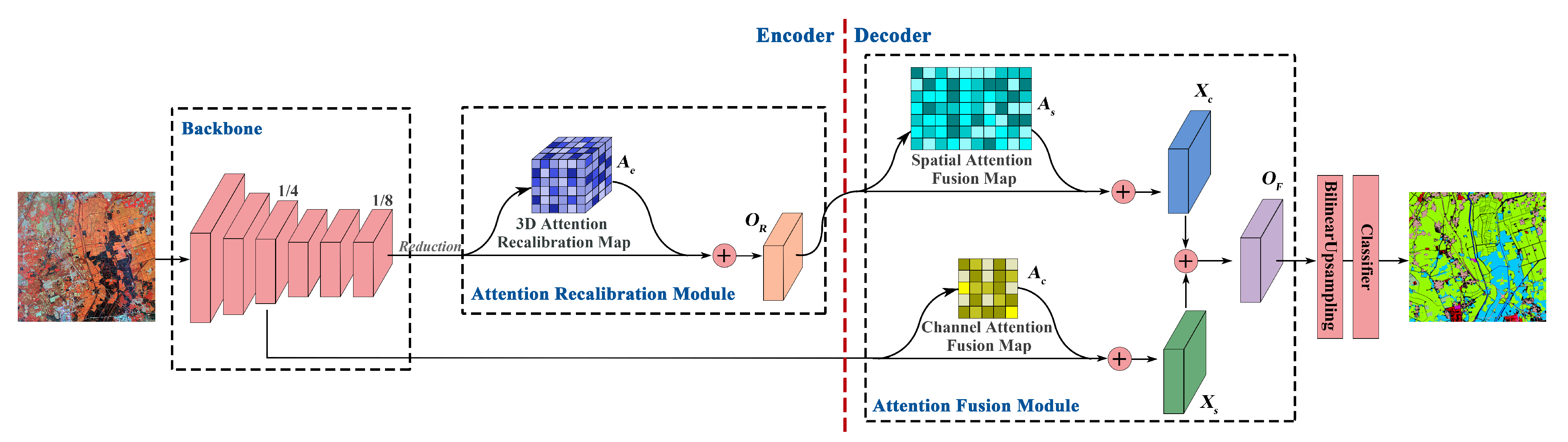
In order to investigate the effect of ARM, we employ the baseline network for ablation experiments, and utilize four state-of-the-art attention modules, including a channel attention module SE [25], a spatial attention module NLN [26] as well as two CS attention modules CBAM [50] and DANet [32], for comparisons. In the implementation of experiments, these attention modules are inserted into the bottleneck of the baseline network, i.e., the position of ARM in XANet, as shown in Figure 1. 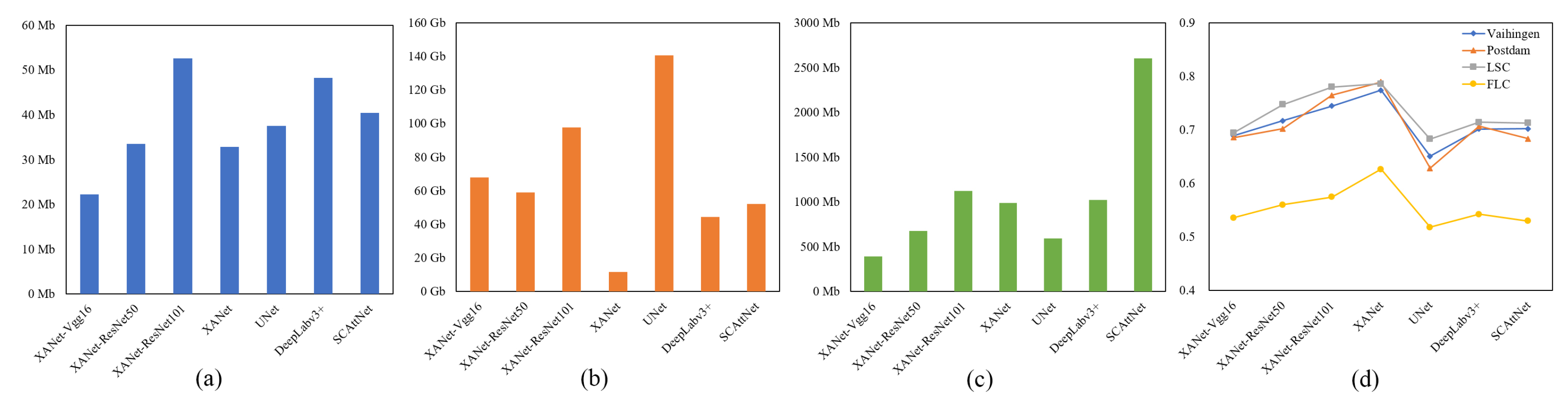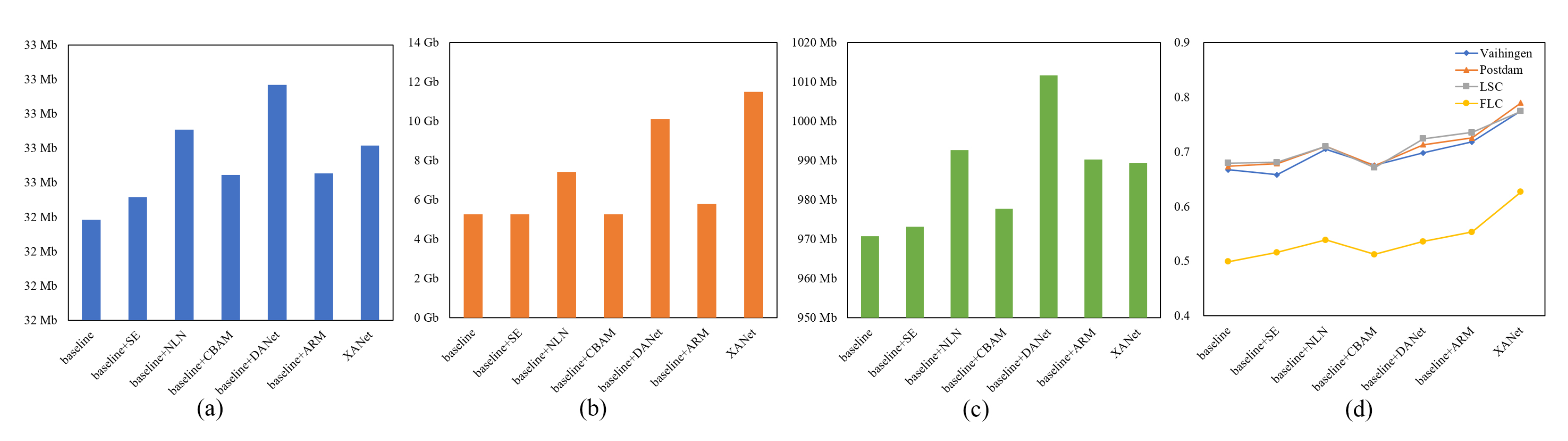Figure 10 sketches the comprehensive comparison of these attention modules from many aspects.

Table 3. Complexity comparison of different attention modules.

	Baseline	Baseline+SE	Baseline+NLN	Baseline+CBAM	Baseline+DANet	Baseline+ARM	XANet
Params (MB)	32.38	32.51	32.91	32.64	33.17	32.65	32.81
Flops (GB)	5.25	5.25	7.40	5.25	10.08	5.79	11.49
Memory (MB)	970.65	973.16	992.65	977.70	1011.65	990.19	989.31

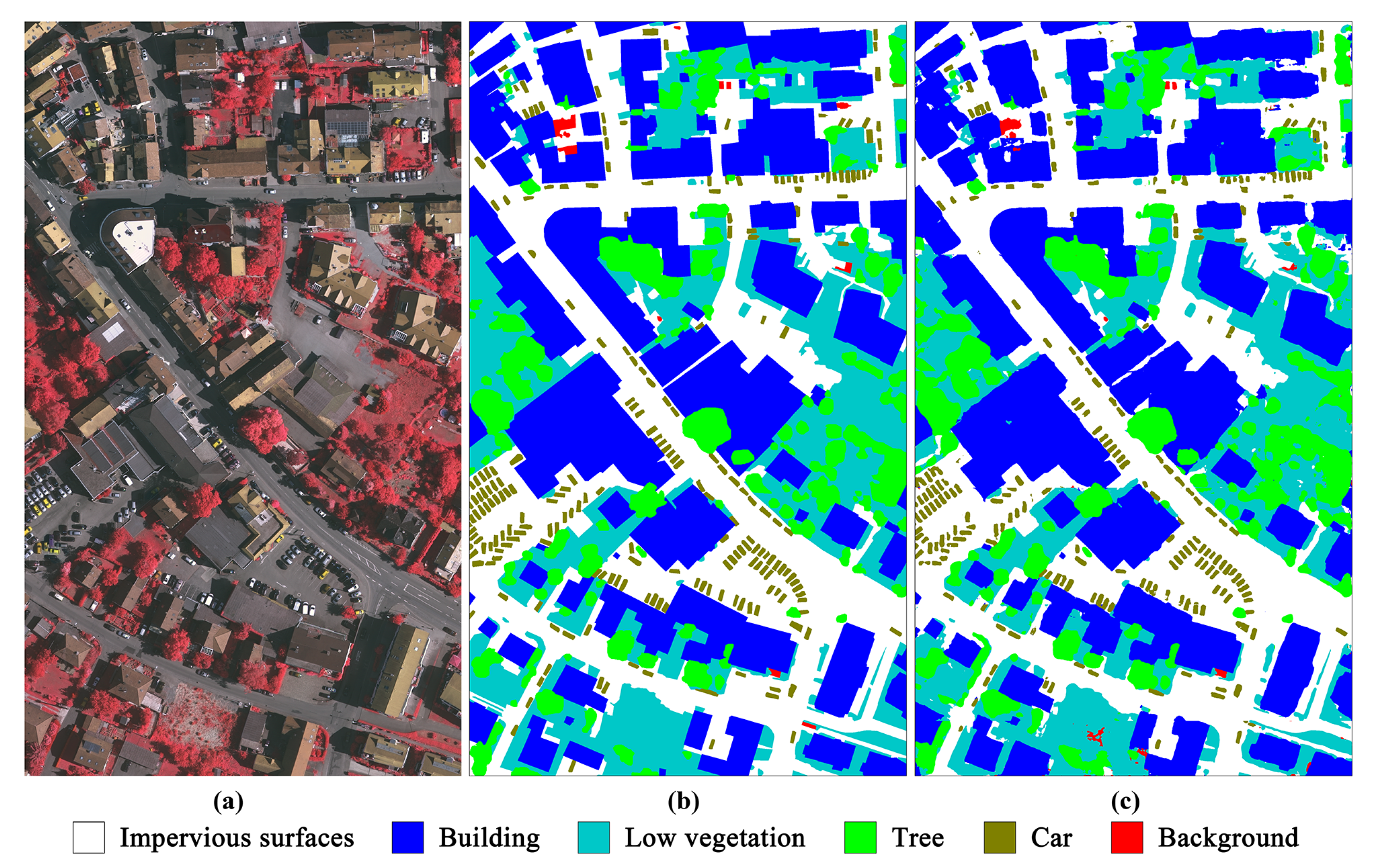
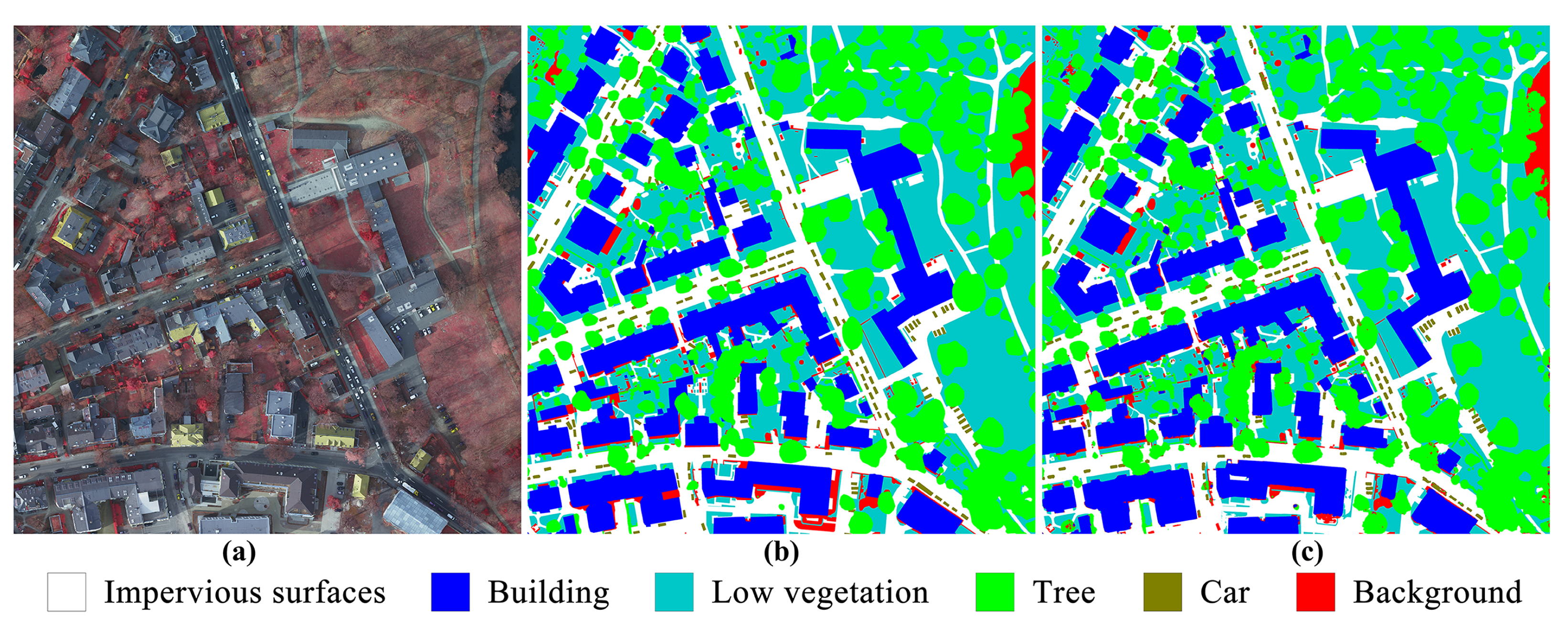
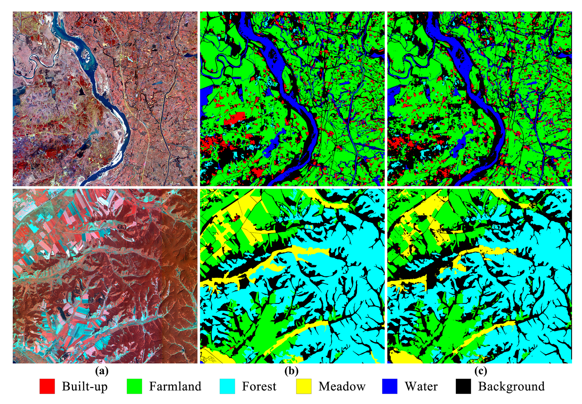
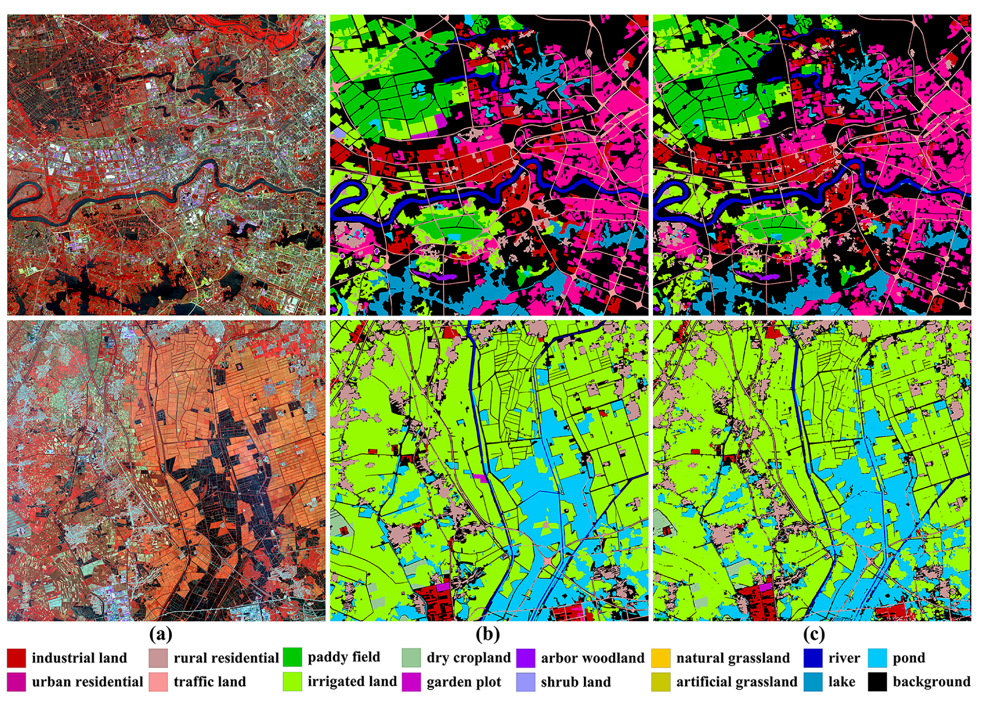
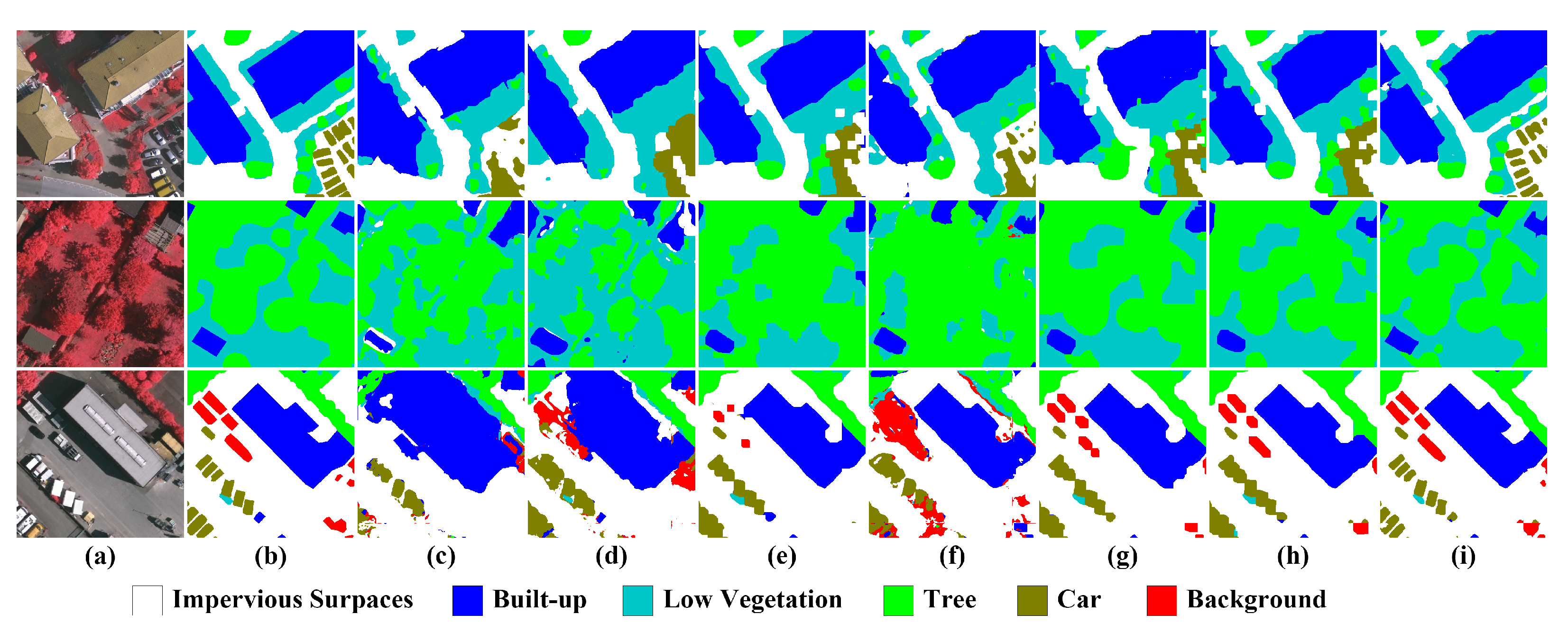
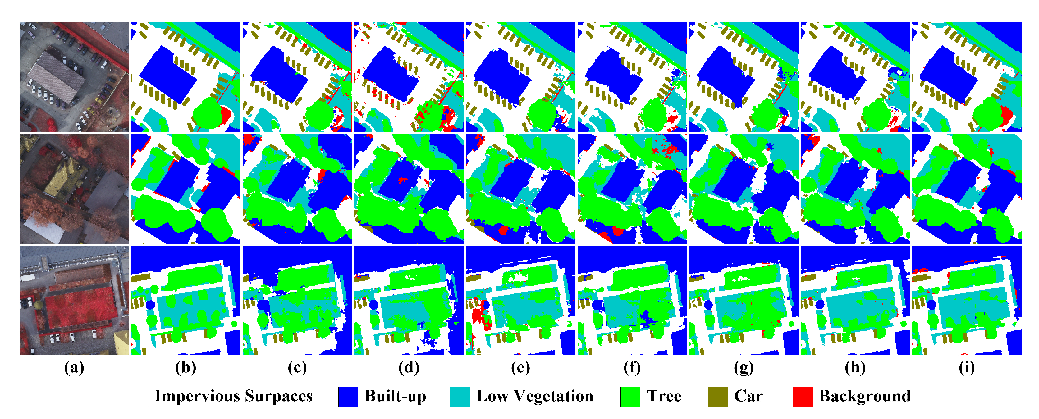
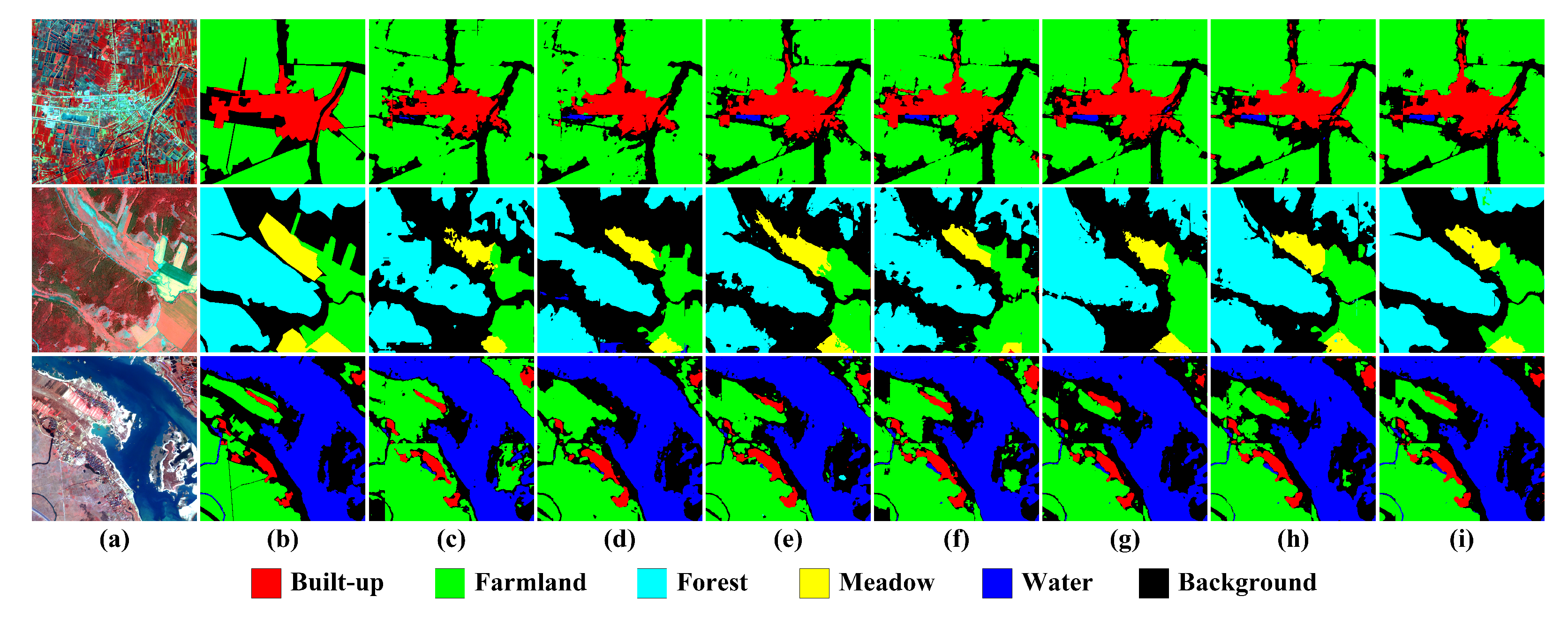
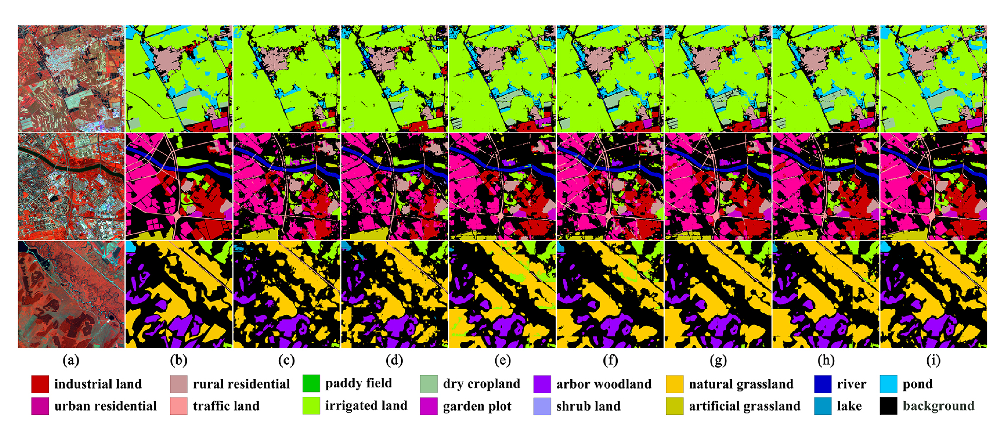
compares their model complexity. Figure 11, Figure 12, Figure 13 and Figure 14 depict the examples of their segmentation results on the four datasets, and

Table 4. Accuracy comparison of different attention modules on the Vaihingen dataset.

	IS	Building	LV	Tree	Car	mIoU
baseline	0.7750	0.7260	0.6350	0.6758	0.5233	0.6670
baseline+SE	0.7843	0.7307	0.6620	0.6331	0.4793	0.6579
baseline+NLN	0.8171	0.7854	0.6475	0.7065	0.5665	0.7046
baseline+CBAM	0.8150	0.8132	0.6059	0.6259	0.5147	0.6749
baseline+DANet	0.7866	0.7643	0.6761	0.7130	0.5490	0.6978
baseline+ARM	0.8235	0.8030	0.6718	0.7160	0.5753	0.7179
XANet	0.8573	0.8782	0.7251	0.7543	0.6559	0.7742

,

Table 5. Accuracy comparison of different attention modules on the Postdam dataset.

	IS	Building	LV	Tree	Car	mIoU
baseline	0.7825	0.7140	0.6520	0.6254	0.5920	0.6732
baseline+SE	0.7968	0.7314	0.6873	0.6120	0.5640	0.6783
baseline+NLN	0.8030	0.7820	0.6629	0.6536	0.6483	0.7100
baseline+CBAM	0.8035	0.7354	0.6248	0.6084	0.6015	0.6747
baseline+DANet	0.7882	0.7733	0.6829	0.6644	0.6564	0.7131
baseline+ARM	0.8177	0.8032	0.6964	0.6726	0.6366	0.7253
XANet	0.8539	0.8550	0.7263	0.7434	0.7689	0.7895

,

Table 6. Accuracy comparison of different attention modules on the LSC dataset.

	Built-Up	Farmland	Forest	Meadow	Water	mIoU
baseline	0.5635	0.7970	0.5944	0.5838	0.8571	0.6792
baseline+SE	0.5211	0.8217	0.6280	0.5971	0.8361	0.6808
baseline+NLN	0.6571	0.8149	0.6107	0.5803	0.8854	0.7097
baseline+CBAM	0.5567	0.8007	0.5633	0.5612	0.8744	0.6713
baseline+DANet	0.6460	0.8271	0.6580	0.6182	0.8689	0.7236
baseline+ARM	0.6389	0.8324	0.6970	0.6260	0.8813	0.7351
XANet	0.7244	0.8648	0.7282	0.6523	0.8992	0.7738

and

Table 7. Accuracy comparison of different attention modules on the FLC dataset.

	IDL	UR	RR	TL	PF	IGL	DC	GP	AW	SL	NG	AG	River	Lake	Pond	mIoU
baseline	0.5950	0.7220	0.6063	0.6171	0.5494	0.7626	0.6135	0.0428	0.6342	0.0676	0.6592	0.1710	0.6448	0.6120	0.1860	0.4989
baseline+SE	0.6073	0.7454	0.6104	0.5130	0.6071	0.8022	0.6393	0.0088	0.6585	0.0470	0.6925	0.2457	0.6629	0.6873	0.2078	0.5157
baseline+NLN	0.6566	0.7535	0.6657	0.6450	0.5694	0.7890	0.6717	0.1643	0.6451	0.1873	0.6265	0.0510	0.7015	0.6971	0.2544	0.5385
baseline+CBAM	0.6130	0.7395	0.6220	0.6717	0.5580	0.7618	0.6823	0.0816	0.6591	0.0860	0.6613	0.1350	0.6243	0.6451	0.1433	0.5123
baseline+DANet	0.6611	0.7355	0.6208	0.6374	0.5774	0.7964	0.6537	0.1645	0.6477	0.2097	0.6724	0.1439	0.6753	0.6739	0.1674	0.5358
baseline+ARM	0.6627	0.7849	0.6363	0.6561	0.5745	0.7782	0.6495	0.1913	0.6653	0.2048	0.6674	0.2246	0.7144	0.6586	0.2320	0.5534
XANet	0.7362	0.8571	0.7132	0.7523	0.6554	0.8572	0.7269	0.2622	0.7156	0.2863	0.7068	0.2753	0.7741	0.7076	0.3725	0.6266

display their accuracy results on the four datasets. The following will concretely investigate the feature enhancement ability of each attention module through ablation studies, and explore the advantages of ARM over other attention modules via comparison studies.

SE: In spite of a small increment in computational overhead, as shown in Table 3 and Figure 10a–c, the use of SE does not involve noticeable gains in the overall accuracy of each dataset and even brings about the negative growth of $mIoU$ on the Vaihingen dataset, as shown in Figure 10d. Specifically, as shown in Table 4, Table 5, Table 6 and Table 7, SE outperforms other attention modules on some categories on the FLC dataset, and can also effectively improve the extraction of some large-scale categories and several categories strongly influenced by spectral information on the other dataset, such as Low Vegetation on the Vaihingen and Postdam datasets, as well as Farmland and Forest on the LSC dataset. However, as a whole, its improvement to most categories on each dataset is limited, even leading to obvious decreases in $IoU$. The experimental results indicate that the channel descriptors under the global receptive field are too coarse to effectively enhance the feature map from the channel dimension, which to some extent even impairs the class discriminative ability.

NLN: It obtains a significant performance improvement on each dataset, with increases in $mIoU$ ranging from 3.0% to 4.0%, as shown in Figure 10d, however, the model complexity is only better than that of DANet, as shown in Table 3 and Figure 10a–c. NLN models the spatial interdependencies between any two positions in spatial dimensions. The accuracy results of categories with obvious context information are greatly improved, such as Building and Car on the Vaihingen and Postdam datasets, as well as Built-Up on the LSC dataset, as shown in Table 4, Table 5 and Table 6. Furthermore, unlike pooling and convolutional layers, where the receptive fields are fixed and local, NLN can capture spatial information in a more adaptable manner. Consequently, the $IoU$ of categories with distinct yet irregular boundaries can also obtain significant gains, such as Water on the LSC dataset, as well as $River$, $Lake$ and $Pond$ on the FLC dataset, as shown in Table 7. However, this way of aggregating spatial context information, which considers the influence of all locations to themselves but disregards channel information, also reduces the inter-class separability between categories with spatial adjacency or semantic similarity to a certain degree, such as Artificial Grassland and Natural Grassland on the FLC dataset. In conclusion, NLN can bring about effective feature enhancement by further encoding spatial dependencies, but given the prohibitive model complexity and the negative impacts on some categories, it still needs additional development.

CBAM: With the similar thinking of SE, per-channel and per-pixel descriptors are aggregated using max and average pooling operations, and then spatial and channel relationships are further modeled with convolutional and FC layers, respectively. However, the performance of CBAM is inferior to that of SE on the three datasets except the Vaihingen dataset, and its $mIoU$ is even lower than that of the baseline on the LSC dataset, as shown in Figure 10d. We contend that the way of gathering the spatial descriptors may be detrimental to channel enhancement to some extent, hence impairing class discriminative ability. However, there are still great performance gains in some large-scale categories with distinct boundaries, such as Impervious Surfaces and Building on the Vaihingen and Postdam datasets, as shown in Table 4 and Table 5. To sum up, despite its enhancement in terms of both spatial and channel dimensions requiring low computational overhead, the performance improvement of CBAM is too limited to be directly employed as the efficient feature enhancement module for remote sensing image segmentation.

DANet: It calculates the pairwise correlations of channels and pixels, respectively, and the three model complexity evaluation criteria are all up to the maximum. However, the $mIoU$ of DANet is superior to that of NLN only on the LSC dataset, as shown in Figure 10d, and its improvement in some categories with obvious spatial context information is also not as significant as that of NLN, such as Impervious Surfaces and Building on the Vaihingen and Postdam datasets, Built-Up on the LSC dataset, as well as Urban Residential and Rural Residential on the FLC dataset, as shown in Table 4, Table 5, Table 6 and Table 7. On the other hand, its performance on several categories with a greater reliance on spectral information is still remarkable, even reaching the best values among all attention modules such as Low Vegetation on the Vaihingen dataset, and Shrub Land on the FLC dataset. In summary, although the improvement in the baseline+DANet over the baseline is outstanding, DANet does not show absolute advantages over NLN, neither in terms of overall accuracy nor in the extraction of some categories, as shown in Figure 10. Meanwhile, taking its huge computational overhead into consideration, it cannot be a viable option for feature enhancement in the real applications of remote sensing.

DANet: It calculates the pairwise correlations of channels and pixels, respectively, and the three model complexity evaluation criteria are all up to the maximum. However, the $mIoU$ of DANet is superior to that of NLN only on the LSC dataset, as shown in Figure 10d, and its improvement in some categories with obvious spatial context information is also not as significant as that of NLN, such as Impervious Surfaces and Building on the Vaihingen and Postdam datasets, Built-Up on the LSC dataset, as well as Urban Residential and Rural Residential on the FLC dataset, as shown in Table 4, Table 5, Table 6 and Table 7. On the other hand, its performance on several categories with a greater reliance on spectral information is still remarkable, even reaching the best values among all attention modules such as Low Vegetation on the Vaihingen dataset, and Shrub Land on the FLC dataset. In summary, although the improvement in the baseline+DANet over the baseline is outstanding, DANet does not show absolute advantages over NLN, neither in terms of overall accuracy nor in the extraction of some categories, as shown in Figure 10. Meanwhile, taking its huge computational overhead into consideration, it cannot be a viable option for feature enhancement in the real applications of remote sensing.

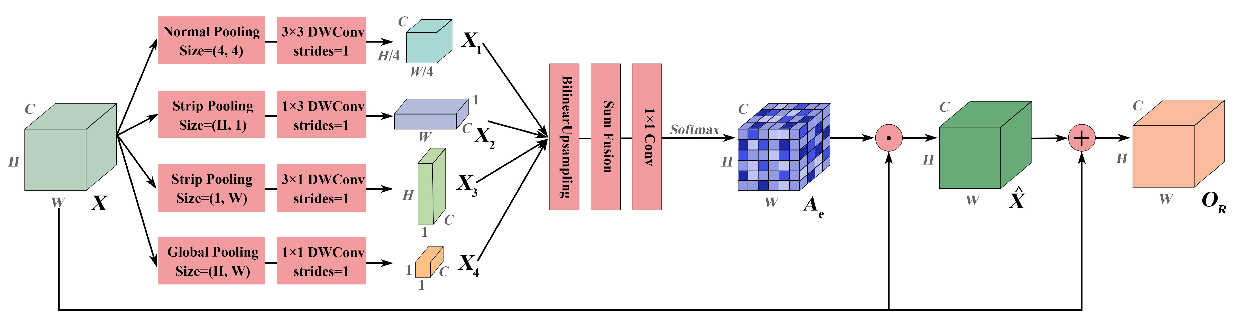
ARM: In lieu of computing the covariance matrix of pixels for the spatial similarity, it employs three types of pooling operations to probe spatial correlations, and also summarizes channel descriptors under different receptive fields in the meantime. In terms of model complexity, as shown in Table 3 and Figure 10a–c, the GPU memory usage of ARM is between NLN and DANet, the model parameters almost match those of CBAM, and the computational complexity, i.e., $FLOPs$, is lower than that of NLN. In terms of model performance, it ameliorates the $mIoU$ of each dataset to the greatest extent, as shown in Figure 10d. Specifically, different-range spatial dependencies captured by ARM contribute to the extraction of multi-scale and multi-shape categories, as shown in Table 4, Table 5, Table 6 and Table 7, thus allowing it to perform better than other attention modules on these categories. Moreover, the channel descriptors under different receptive fields can determine channel relationships more precisely and enable a more significant enhancement of semantic and discriminative information. Thus, ARM can also provide the more prominent improvement in some categories greatly influenced by spectral information. Therefore, taking efficiency and effectiveness into account, ARM has noticeable advantages over other state-of-the-art attention modules, and contributes more to the simple yet effective segmentation for remote sensing imagery.

In summary, with the aid of flexible receptive fields provided by three-type pooling operations, our proposed attention module for improving the encoder, namely ARM, can extract outstanding semantic descriptors to generate the element-wise 3D attention map, effectively enhancing a feature map from both spatial and channel dimensions at the same time. The comparison of the baseline and the baseline + ARM reveals that ARM can yield significant performance gains for each category with slight increases in model complexity. Additionally, ARM can also surpass other state-of-the-art attention modules in terms of overall accuracy and the most category extraction, and its model complexity remains competitive among these modules as well. The improvement of the baseline + ARM over the baseline and the advantages of ARM over other attention modules both demonstrate the effectiveness of ARM. Furthermore, as a better compromise between model performance and complexity, ARM is more conducive to fulfilling the high-accuracy and high-efficiency requirements in real-world remote sensing scenarios.

5.2. Effect of AFM

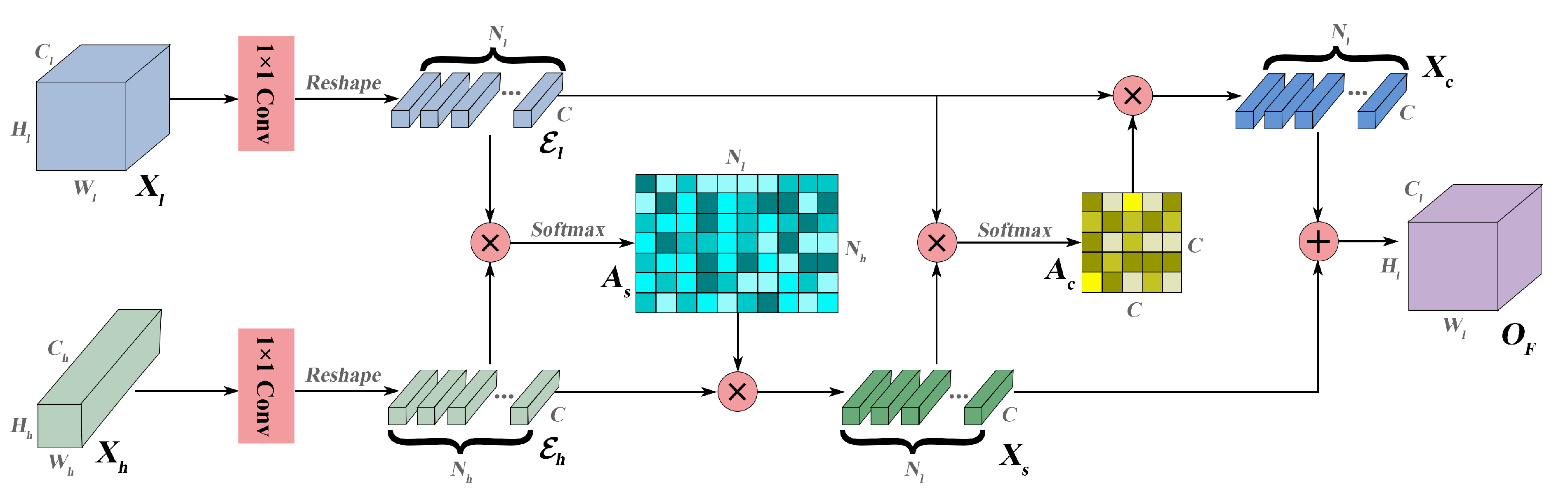
As mentioned in Section 3.3, AFM achieves the spatial and channel fusion of low-level and high-level features via cross-attention, and the channel- and spatial-fused features are further merged by the addition operation. In this subsection, we not only investigate the effect of AFM by comparing the baseline+ARM with XANet, as shown in Table 4, Table 5, Table 6 and Table 7 and Figure 11, Figure 12, Figure 13 and Figure 14, but also explore the specific role of each component in AFM through further ablation studies, as shown in

Table 8. Ablation studies of each component in AFM.

Method	Spatial Attention Fusion	Channel Attention Fusion	Vaihingen	Postdam	LSC	FLC
baseline+ARM			0.7179	0.7093	0.7351	0.5534
baseline+ARM+AFM_1			0.7233	0.7126	0.7244	0.5481
baseline+ARM+AFM_2	√		0.7523	0.7543	0.7554	0.6088
baseline+ARM+AFM_3		√	0.7316	0.7339	0.7676	0.5832
XANet	√	√	0.7742	0.7735	0.7861	0.6266

. Three fusion modules are additionally implemented. AFM_1 only performs the sum fusion, after unifying the channel numbers of two-level features with two $1\times 1$ convolutions and enlarging the spatial size of the high-level feature to that of the low-level feature with a bilinear upsampling operation. AFM_2 and ARM_3 are constructed by removing the channel and spatial attention fusion from AFM, respectively. The following will elaborate on the ability of each fusion module, and analyze the effectiveness and efficiency of AFM.

First of all, in terms of model complexity, as shown in Table 3 and Figure 10a–c, compared with the baseline + ARM, although the $FLOPs$ of XANet are almost doubled with the addition of AFM, the increases in model size are negligible, and the required computational resources even decline due to its dimension-reduced operations. In general, AFM does not impose a huge computational burden.

Then, we discuss the performance of AFM through the improvement of XANet over the baseline+ARM. Specifically, as shown in Table 4 and Table 5, on the Vaihingen and Postdam datasets, some categories that are obviously influenced by spatial context information, such as Building and Car, are improved to a great extent after further feature fusion with AFM. Additionally, Tree on the Postdam dataset with rich texture information also obtains significant performance gains, owing to the detail information highlighted by AFM. On the LSC dataset, as shown in Table 6, the $IoU$ of Built-Up increases sharply due to the enhancement of texture and context information from the spatial attention fusion in AFM, and the channel attention fusion, which improves object semantic and discriminative information, further promotes the performance improvement of each category extraction. On the FLC dataset with the finer category system, as shown in Table 7, AFM also brings great performance growth since the texture and detail information have become pivotal for distinguishing many categories from each other.

At last, the specific role of each component in AFM is explored by further ablation studies, as shown in Table 8. Intuitively, comparing the baseline + ARM + AFM_1 with the baseline + ARM, AFM_1 without any attention fusion cannot provide significant improvement and even has negative impacts, indicating that the poor fusion strategy may be detrimental to the model performance. AFM_2 only employs the spatial attention fusion for the two-level features, which contributes to restoring the detailed information for pixel-level predictions, and its performance gains are second only to those of AFM on most datasets. Furthermore, benefiting from the enhancement of semantic and discriminative information brought by the channel attention fusion, the improvement of AFM_3 is also noticeable on each dataset, and the performance growth on the LSC dataset even exceeds that of AFM_2, which reveals the importance of performing an effective channel fusion strategy. Furthermore, in general, AFM effectively realizes the complementary advantages of the two-level features, and its improvement on each dataset is much better than that of other fusion modules, which illustrates that spatial and channel fusion are both indispensable, and the combination can yield the superior performance.

In summary, multi-level feature fusion is crucial for fine-grained remote sensing image segmentation, while a poor fusion strategy is susceptible to detrimental effects. The spatial and channel attention fusion in AFM can both bring about good performance gains, where the former improves the class discriminative ability and the latter remedies the spatial information losses. AFM, integrating the advantages of fusion in two aspects, becomes an outstanding strategy for efficient feature fusion, which can make full use of multi-scale information from different-level features for accurate pixel-level predictions without substantially increasing the model complexity.

5.3. Model Interpretability

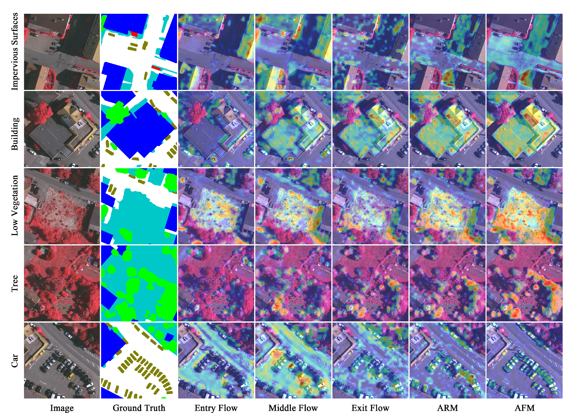
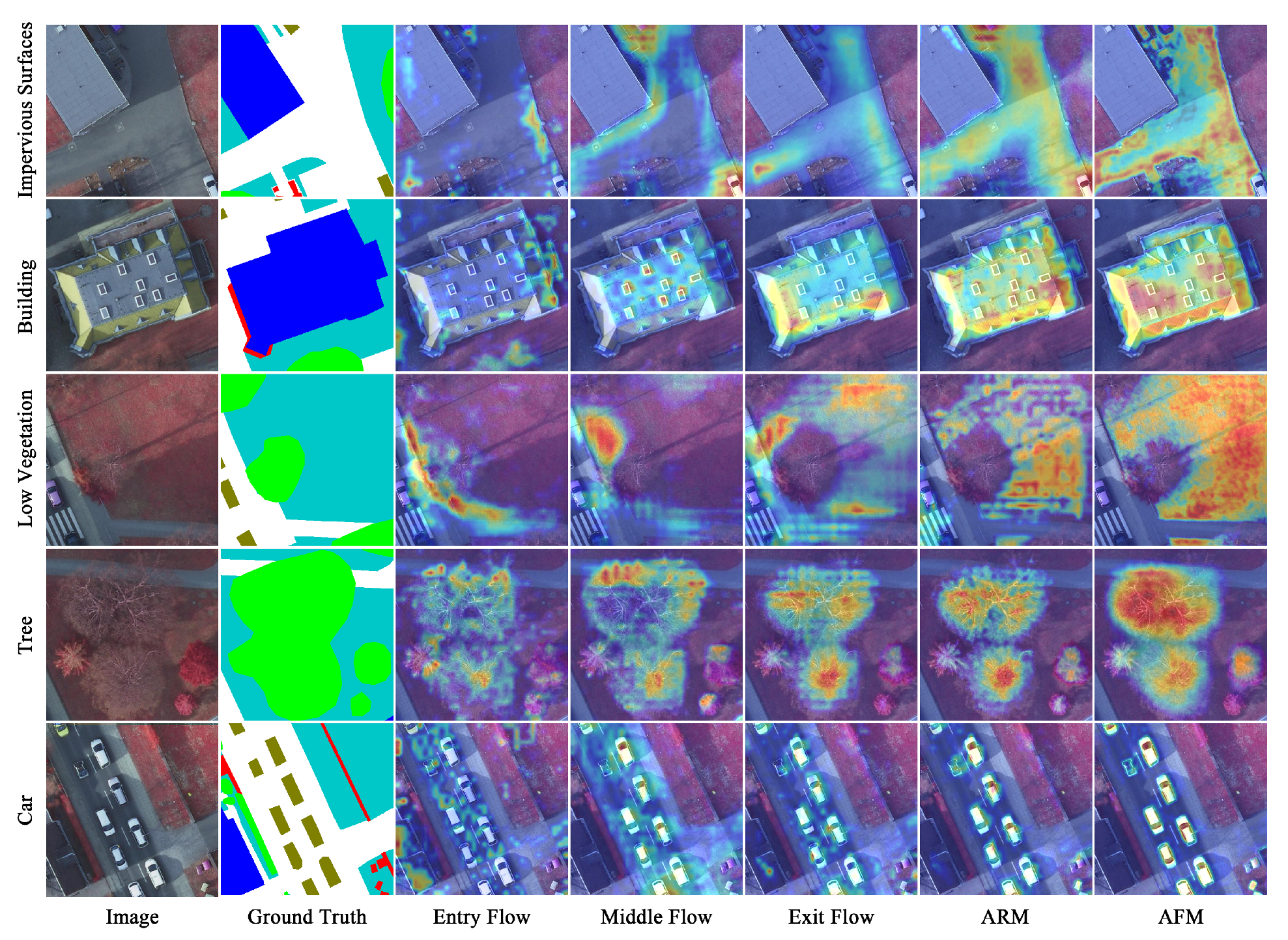
Chollet [57] divided Xception65 into Entry Flow, Middle Flow and Exit Flow. Consequently, we consider the reasoning process of XANet as five phases, i.e., the three phases from the backbone network, as well as ARM and AFM. In order to figure out the reasoning mode of our hierarchical segmentation model and further intuitively analyze the two proposed attention modules, this section employs the Grad-CAM tool, which can clarify the regions considered important by the current network layer for a certain category in the form of a heat map, to visualize the output feature of each phase with regard to each category on the Vaihingen and Postdam datasets, as shown in Figure 15 and Figure 16, respectively.

In the Entry Flow phase, for some categories, the feature is activated on external context information, such as the buildings adjacent to the Impervious Surfaces on the Vaihingen dataset, and the roads where the Car is on the two datasets. For a Building with clear boundaries on the two datasets, some obvious edge information is highlighted as well. Furthermore, for Low Vegetation on the Vaihingen dataset and Tree on the Postdam dataset, a small amount of texture information is also focused to a certain degree. In the Middle Flow and Exit Flow phases, as the network goes deeper, the feature concentrates more on the category itself and less on the background, and the emphasis of each category gradually shifts to the internal texture information. After the enhancement of ARM, the discriminative information of each category is further significantly boosted, the influence of other categories is effectively suppressed, and the recognizable texture information is more abundant. After improvement with AFM, there is the stronger response to each category, and the feature activates itself almost exclusively on each category, especially Car on the two datasets.

Altogether, in the reasoning process of XANet, external spatial position information, edge information and internal texture information are successively extracted with the deepening of the network, and identifiable discriminative information is less-to-more and coarse-to-fine. The improvement of ARM and AFM is also manifestly reflected by the Grad-CAM. Intuitively, ARM can effectively recalibrate the focus on each category, and improve the class discriminative ability of a feature map. AFM further boosts the response to each category and represses the interference from other categories, especially the small-scale category, which is significantly ameliorated.

6. Conclusions

In response to time-sensitive interdisciplinary applications and large data volumes in the remote sensing field, this paper aimed to propose a more effective segmentation model to perform fine-grained image interpretation at a faster processing speed. Through the cause analysis of the high accuracy and high consumption of the most popular CNN-based Encoder–Decoder segmentation models, we employ the attention mechanism which was well received in NLP to strike a better balance between the model performance and complexity. Two efficient attention modules, namely ARM and AFM, were proposed for element-wise feature enhancement in the encoder and multi-scale information fusion in the decoder, respectively. Equipped with them, a simple yet effective segmentation model, termed XANet, is constructed accordingly. Extensive comparison and ablation experiments were conducted on the ISPRS and GID datasets for the comprehensive analysis of XANet, ARM and AFM. Furthermore, the following conclusions can be drawn:

• XANet has good model scalability in several backbone networks, and compared with other state-of-the-art segmentation models, it can achieve better model performance with lower model complexity. Additionally, with the help of the Grad-CAM tool, we gain a deeper understanding of the reasoning mode of XANet, inferring the external-to-internal identification strategy, as well as the less-to-more and coarse-to-fine information acquisition approach.
• ARM aggregates outstanding semantic descriptors under multi-scale receptive fields, which can concurrently summarize spatial and channel information to directly excite an element-wise 3D recalibration attention map. In relevant experiments, ARM brings more significant performance gains over other state-of-the-art attention modules with very competitive model complexity, which verifies its effectiveness and efficiency. Furthermore, the changes in saliency maps visualized by Grad-CAM before and after ARM also further illustrate its feature enhancement ability.
• AFM pioneers the use of the cross-attention mechanism for multi-scale feature fusion in image segmentation. We empirically demonstrate that a good fusion strategy is of importance for pixel-level predictions, that both the spatial and channel attention fusion in AFM can effectively boost performance, and that AFM can integrate their advantages for better improvement without significant increases in computational overhead. Furthermore, Grad-CAM visualization maps before and after AFM more intuitively illustrate its effectiveness in fine-grained segmentation.

XANet equipped with the two proposed attention modules has achieved prominent performance without huge computational overhead. However, our segmentation model still employs a CNN-based backbone network for primary feature extraction, and the convolution process itself is an inefficient information aggregation with fixed filters. In response to the limitations of convolutions, some pure attention vision models—established only by the attentional layer—have been developed to capture visual information in a more efficient manner, and have achieved better performance than CNN-based models in many coarse-grained CV tasks. Inspired by these successful attempts, in the future, we will further explore the feasibility of a fully attentional model in remote sensing image segmentation, and investigate the advantages and disadvantages of the attentional layer compared with the convolutional layer in the remote sensing field.