Abstract
The monitoring of irrigated areas still represents a complex and laborious challenge in land use classification. The extent and location of irrigated areas vary in both methodology and scale. One major reason for discrepancies is the choice of spatial resolution. This study evaluates the influence of spatial resolution on the mapped extent and spatial patterns of irrigation using an NDVI threshold approach with Sentinel-2 and operational PROBA-V data. The influence of resolution on irrigation mapping was analyzed in the USA, China and Sudan to cover a broad range of agricultural systems by comparing results from original 10 m Sentinel-2 data with mapped coarser results at 20 m, 40 m, 60 m, 100 m, 300 m, 600 m and 1000 m and with results from PROBA-V. While the mapped irrigated area in China is constant independent of resolution, it decreases in Sudan (−29%) and the USA (−48%). The differences in the mapping result can largely be explained by the spatial arrangement of the irrigated pixels at a fine resolution. The calculation of landscape metrics in the three regions shows that the Landscape Shape Index (LSI) can explain the loss of irrigated area from 10 m to 300 m (r > 0.9).
1. Introduction
Remote sensing has proven to be a suitable instrument for land use classification and land surface monitoring. The time series of remote sensing data allow for detecting land use change and changes in agricultural patterns and management practices. Agriculture uses vast amounts of natural resources such as fresh water for irrigation in an often-non-sustainable way [1]. To secure current and future global food supplies in a sustainable way, agriculture has to increase the efficiency of the water it uses, which is expressed in the principle of “more crop per drop” [2]. Developing and finally establishing monitoring capabilities for agricultural irrigation and its efficiency therefore constitutes a major prerequisite towards improving the efficiency, effectiveness and sustainability of agricultural water use.
Remote sensing is the central data source for a quantitative global, regional and local monitoring of areal extent, timing and technique of irrigation. The Copernicus Sentinel missions provide, on an operational basis, high spatial and temporal resolution data. Together with increasing computing capacities, they extend our Earth observation capacities to develop and deploy the monitoring systems necessary to achieve the necessary efficiency gains in irrigation.
Since approx. 20% of the total cropland is irrigated and approx. 40% of the world food is produced on this cropland, irrigation plays a crucial role in global food production [3]. Irrigated cropland consumes 69% of the global water withdrawal from surface and groundwater [4]. Global irrigated area doubled in the last 50 years [3] and future expansion is expected [5,6]. Over 50% of the irrigated areas are located in regions characterized by annual precipitation smaller than 750 mm, which is considered the limit below which diverse demands for water may lead to allocation conflicts [7,8]. Additionally, the impact of climate change may regionally influence precipitation and snowmelt patterns and, consequently, river flows and groundwater recharge, and may thus reduce the availability of fresh water, aggravate water scarcity and amplify water-related conflicts [8].
The high demand for irrigation water strains the regional hydrological cycle mainly through withdrawal from local and regional rivers and aquifers. Irrigation water is diverted into the atmosphere and, as a result, lost for further downstream uses. Dramatic reductions in run-off and aquifer levels caused by irrigation with adverse effects for the regional environment and for the downstream population are documented worldwide [9,10,11,12]. It is, therefore, crucial to monitor, with high accuracy, the location and extent of irrigated area.
Mapping of irrigated areas still represents a challenge for remote sensing. Several studies have shown the feasibility of mapping irrigated areas using remote sensing data from the local to global scale [13,14,15,16,17,18]. Existing irrigation mapping methods combine different data to exclude rain-fed and irrigated land by strong indicators such as evapotranspiration [19], climatic conditions [17], thermal variations over an irrigated field [20] or soil moisture [21]. The few existing global studies about irrigated areas show large differences in its extent and spatial pattern and are subject to controversial discussions in the scientific community [22,23]. The differences are caused by different assumptions and definitions, different time periods and data from different satellite missions with different spatial resolution and spectral coverage. This study focusses on the influence of spatial resolution of remote sensing data on the resulting location and extent of derived irrigated areas. Velpuri et al. [24] already showed, in a case study, that finer spatial resolution can result in an increase in classified irrigated area. They conclude that current operational irrigation monitoring systems, which are based on coarser resolution imagery from, e.g., AVHRR, MODIS or PROBA-V, neglect relevant parts of the global irrigated area [24]. Nevertheless, they do not address the transferability of their findings to other regions. On the other hand, coarser resolution has convincing advantages for global monitoring systems of the temporal development of global irrigation, such as daily global coverage and low data rates.
The existing long time series of medium-resolution LANDSAT data and the new medium spatial and high-temporal-resolution Sentinel-2 data have successfully been used in regional and local studies to determine the extent of irrigated areas with high precision [25,26,27]. In principle, they would be the data source of choice for a more complete, global, operational irrigation mapping. Sentinel-2 now allows, in principle, to precisely and operationally resolve, with high spatial resolution, the temporal NDVI-developments on which current approaches to distinguish irrigated areas from non-irrigated areas rely. Improved global irrigation monitoring therefore seems possible but not feasible considering the massive computational resources necessary to analyze frequent time series of large areas with high spatial resolution. This may be one reason why, despite the anticipated added precision, to our knowledge, operational irrigation monitoring on a global scale using Sentinel-2-time series is not available yet.
On the other hand, Sentinel-2 time series could potentially be used to augment existing global low-resolution approaches to map irrigated areas, given that the local scaling laws, which govern the change in detected irrigated areas with decreased spatial resolution, are well understood. The hypothesis of our paper, therefore, is that the change in detected irrigated areas with decreasing spatial resolution inherent in the current approaches follows a regional independent scaling relation. We consider the resulting scaling relations as a property of the plot size, the spatial arrangement and the complexity of the shape of the irrigated fields. The complexity of the spatial structure of the irrigated areas can be described by landscape metrics, well known from biodiversity and habitat analysis [28,29]. The Landscape Shape Index (LSI) was identified to be suitable for explaining the negative changes in the mapping results [30,31,32]. A proven correlating functional relation between the differences in the mapping results caused by resolution and the LSI can be used for estimating the accuracy of global low-resolution irrigation monitoring. In order to investigate the scaling properties, we use a proven approach to globally monitor irrigated areas using NDVI time series, which have been widely used with wide-swath low-resolution sensors such as MERIS and PROBA-V [7]. For the first time, we systematically analyze the impact of spatial resolution from 10 m to 1 km on the pattern and extent of irrigated areas in three selected global regions. We consider different geographical conditions with respect to climate and farming systems by selecting as case studies regions in Sudan, China and the USA.
2. Materials and Methods
2.1. Multi-Resolution Analysis
We applied the method described in Meier, Zabel and Mauser [7] to determine irrigated area. It does not explicitly use spatial resolution as a parameter. The basis of the mapping method is annual NDVI time series. They are used together with parameters such as land suitability for agriculture, a land use classification, NDVI data and official national statistics to determine global irrigated area. The annual course of NDVI is analyzed, interpreted and compared with agricultural suitability evaluations [7,33]. The method analyzes the NDVI time series using parameters such as amplitude of the NDVI, position of NDVI peaks and shape of the NDVI annual temporal course. If the course of NDVI suggests active vegetation growth with typical characteristics of agriculture and, simultaneously, the agricultural suitability is low due to a rainfall deficit, we assume a high likeliness of irrigation. In our case, the original mapping-method [7] is modified in two points to be applicable to the finer spatial resolutions: (1) the information about irrigated area derived from the official statistics are not used to avoid a biased result and (2) the restriction of the approach to only process the land-use cropland is lifted because using an external (coarser resolution) land use classification at this fine spatial resolution would lead to a predetermination of the result. The result of the threshold mapping method is a map containing Boolean information of the status of the field: irrigated or not irrigated.
We derive scaling relation of irrigation extent vs. spatial resolution in three different regions: central Sudan around Khartoum, in northwestern China in the Uighur province Xinjiang and in Colorado, southeast of Denver (Figure 1). These three regions were selected based on the following criteria:
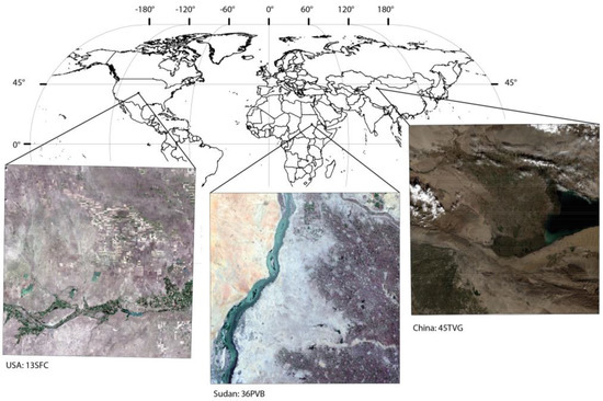
Figure 1.
Global overview of the selected regions including the Sentinel−2 tile name.
- The region’s agricultural suitability is low due to rainfall deficit to avoid both confusion between irrigated and rain-fed areas and high cloud cover.
- The region should be dominated by irrigated agriculture.
- The selected regions should cover a broad range of agricultural systems—from subsistence to high-intensity agriculture.
All three regions are characterized by low annual precipitation values. The region in the USA (303 mm/year) is the wettest, followed by Sudan (202 mm/year) and China (173 mm/year), based on the ERA5 data of the year 2016 [34]. Each study area covers one Sentinel-2 tile of approx. 100 × 100 km.
According to Fritz et al. [35], the field sizes in the three tiles ranges from “very small” to “very large”. The field sizes in the USA are categorized as “large”, in China as “medium” and in Sudan from “very small” to “small”. A visual pre-analysis shows that the sizes and shapes of the fields in China and Sudan vary strongly whereas the fields in the USA are homogeneous and only differ in shape: squared or the typical circular fields shaped by center pivot irrigation. The cultivated crops range from alfalfa and cereals to groundnut and fruits. The area in the USA is characterized by alfalfa (66%) and maize (31%); the remaining agricultural areas are used mainly for fruits and vegetables [36]. The agricultural areas in Sudan are mainly used for the cultivation of groundnut (71%), cotton (8%) and millet (6%). The remaining area of 15% is used for the cultivation of crop types such as maize, cassava, beans, dates and fruits. In the selected China tile, mainly cotton (37%) and maize (32%) are cultivated. Permanent crops such as grapes (4%) and apple trees (3%) are also cultivated, as well as vegetables and fruits.
The study of the scaling relations is carried out for the year 2016. In this study, we apply the modified mapping method described above to the selected Sentinel-2 tiles at a spatial resolution of 10 m, 20 m, 40 m, 60 m, 100 m, 300 m, 600 m and 1000 m to systematically evaluate the impact of spatial resolution on the identified irrigated area. In order to investigate how the Sentinel-2 and PROBA-Vegetation (PROBA-V) spectral coverage compares when using the selected irrigation mapping approach and in order to link the results of the varying-resolution Sentinel-2 mapping with the operational PROBA-V (300 m) mapping of irrigated area, the same irrigation mapping method is also applied to the available PROBA-V data sets of the same period and regions. PROBA-V was developed as successor of SPOT5 to ensure the continuation of low-resolution vegetation products and was successfully launched in 2013. The spectral range is similar to SPOT5 and provides 4 bands (BLUE, RED, NIR, SWIR) in a spatial resolution from 100 to 300 m [37,38]. The Sentinel-2 and PROBA-V results are compared at a spatial resolution of 300 m.
Sentinel-2 is a multi-spectral satellite and is part of the EU’s Copernicus program. The spatial resolution depends on the spectral band. The bands (band 8 (NIR) and band 4 (RED)) used in this study are available at a resolution of 10 m. We use the Top-Of-Atmosphere reflectance (TOA) Sentinel-2 data that are corrected for atmospheric effects to Top-Of-Canopy (TOC) reflectance data at 10 m using an inverse radiative transfer approach based on MODTRAN radiative transfer simulations [39]. During the atmospheric correction process, a cloud and snow mask is automatically derived from the images. All available unmasked data of all available dates of 2016 for the selected tiles are used for our analysis. Figure 2 shows the average number of valid observations per pixel for each month.
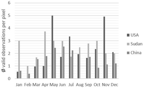
Figure 2.
The average number of valid Sentinel-2 observations per pixel for each month in the study regions.
The Normalized Difference Vegetation Index (NDVI) is calculated from the available Sentinel data where RED is TOC reflectance in band 4 and NIR is TOC reflectance in band 8 as:
This results in a spatially distributed multi-temporal 10 m-resolution temporal course of NDVI covering the year 2016. To calculate multi-temporal NDVI data at 20 m, 40 m, 60 m, 100 m, 300 m, 600 m and 1000 m, the TOC reflectance values of the spectral bands RED and NIR are separately rescaled using a moving window which averages the reflectance of the pixel within the respective area of the coarser resolution. The upscaled reflection value is then used to calculate the NDVI according to Formula 1. For each spatial resolution data set, irrigation maps are created using the identical adapted threshold method to map irrigated areas [7].
2.2. Scaling Relation at Different Spatial Resolution
The irrigation mapping results differ depending on the spatial resolution. Whereas a perfectly homogeneous image does not show differences in NDVI with changing resolution, the averaging of heterogeneous (with reference to the considered resolution) reflectances in the higher resolution images results in a tendency to homogenize the NDVI values in the coarser resolution images. Since the irrigation detection algorithm is non-linear with NDVI, this changes the amount of detected irrigation, with NDVIs averaged over heterogeneous areas. Therefore, we assume a relationship between the heterogeneity of the spatial position and formation of the irrigated area as it is shown in the fine resolution and the area changes when moving up to coarser resolutions. To measure the heterogeneity or homogeneity of the irrigation pattern, we use landscape metrics, a measure for the complexity of a landscape. To quantify the relation between landscape metrics and the areal change with resolution of the mapped irrigated area, we calculate landscape metrics for the three regions. To increase the number of samples, we split each region in 36 tiles to generate more stable statistics. A pre-analysis showed that at and above 6 by 6 pixels, the results remained constant. For the 36 tiles, the areal change between 300 m and 10 m is calculated as follows:
While the pixel at 300 m gives Boolean information (irrigated or not irrigated), the result at 10 m gives more precise information about the irrigated area at the corresponding 300 m pixel. This information is used to determine the difference between the mapping result at 300 m and 10 m. Depending on the position and spatial arrangement of the irrigated area, the change in spatial resolution from 10 m to 300 m can result in positive or negative areal change of irrigated area detected by the algorithm. Negative changes occur in case of a high heterogeneity of the considered area. Positives changes occur when the majority of the considered area is classified as irrigated, and the spectral reflectance is hardly affected by the upscaling process. Positive changes are rather theoretical and hardly ever occur. Therefore, this study will focus solely on the negative changes.
To quantify the relation between landscape metrics and the areal change with resolution of the mapped irrigated area, we calculate landscape metrics on the same 36 tiles of the three regions using the R-package of Hesselbarth et al. [40]. We assume that the position, the shape and the spatial arrangement are reasons for the areal change of the mapping results. To explain the negative changes of irrigated area with decreasing resolution, we calculate the Landscape Shape Index (LSI, see Equation (3)), which describes the ratio of the total edge length of a class, in our case, irrigated area, to the minimum edge length. LSI measures the complexity of a selected class (irrigated) compared to the other classes (not irrigated) of a landscape.
Thus, as a ratio between the actual class edge length and the minimum class edge length, the LSI is an ‘aggregation metric’. In case of only one class in the landscape, the minimum length equals the edge length. The higher the ratio, the more complex the pattern of the irrigated area. The result is a high expected loss of mapped irrigated area at the coarser spatial resolution. The LSI is calculated for the 36 tiles of the irrigation mapping at 300 m and is correlated with the negative areal change for the mapping result between 300 m and 10 m.
3. Results
3.1. Extent of Irrigated Area
The mapped irrigated area as a function of spatial resolutions is compared in Figure 3 for the three selected study sites. Generally, it shows a decrease in irrigated area with decreasing spatial resolution. Nevertheless, there are large differences in the relationship between resolution and area between the selected regions. This can be seen in Figure 3 in China, where the scaling effect is rather small, whereas Sudan and USA show a pronounced scaling effect.
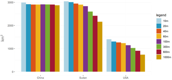
Figure 3.
Mapped irrigated area in the selected Sentinel-2 tiles in China, Sudan and USA at different spatial resolutions. In Sudan and USA, the mapped irrigated area decreases with decreasing spatial resolution while the mapped irrigated area in China is almost independent of resolution.
Table 1 shows the absolute values of the mapped irrigated area in the three study sites in km2 for the selected spatial resolutions.

Table 1.
Resulting irrigated area in the three different regions.
Figure 3 and Table 1 show that the mapping result in China is hardly affected by the upscaling resolution from 10–1000 m. Reasons are the structure of the irrigated area in this region which consists of very large-scale cohesive irrigated plots. In this case, NDVI does not change significantly by averaging towards lower resolutions and a mix of different NDVI values hardly occurs in the high-resolution ensemble underlying the low-resolution pixels.
Figure 4 shows the spatial distribution of the mapped irrigated area in the three selected Sentinel-2 tiles for a spatial resolution of 10 m, 300 m and 1000 m. Visually, the spatial irrigation patterns largely differ in the three regions: while irrigation in Sudan and USA is scattered, the irrigated area in China is more clumped in two large contiguous irrigation clusters. At the coarser spatial resolutions, the small and scattered irrigated areas in Sudan and USA disappear while the irrigated agglomerations in China prevail.
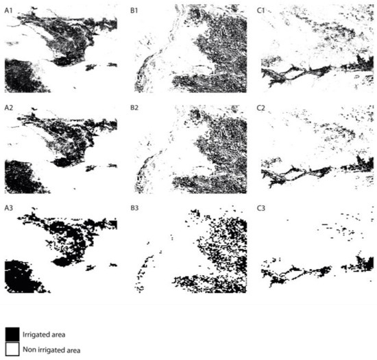
Figure 4.
Mapped irrigated area as a function of spatial resolution in the three different study sites: A = China, B = Sudan, C = USA. 1 = 10 m, 2 = 300 m, 3 = 1000 m.
3.1.1. Sudan
The identified irrigated area in Sudan clearly decreases with coarser spatial resolution. At a resolution of 100 m, the irrigated area decreases by 7% and continues to decrease to 29% at a resolution of 1000 m (Figure 3 and Table 1). At a coarser resolution of 300 m, single small-scale fields are no longer classified as irrigated, especially when they are surrounded by non-cultivated or abandoned fields or non-vegetated areas. This effect decreases the extent of irrigated areas. Figure 5 shows that contiguous clusters of fields are less affected by resolution decrease. At the finer resolutions (below 300 m), the fields are well defined and differentiation between fallow fields, possible artificial area and other irrigated fields is possible. At the coarser resolutions (from 300 m upwards), the areal extent decreases and the original patterns are hardly visible.
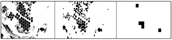
Figure 5.
The decrease in irrigated area at coarser resolutions at the study site in Sudan. The left image shows the area classified as irrigated at the resolution of 10 m. The middle shows the same area at 300 m and at the right at 1000 m.
Figure 5 shows the center pivot fields in the northwestern part of the Sudan tile. This detail serves as a good example of the decrease in the irrigated area. At the finer resolutions, the center pivot fields can clearly be identified. At a resolution of 300 m, the center pivot fields dissolve and almost completely disappear at the resolution of 1000 m.
3.1.2. USA
In the USA, the irrigated area decreases by 27% at the resolution of 300 m and by 48% at the coarsest resolution of 1000 m (Figure 3 and Table 1). At the finest resolution, the irrigated area around the Arkansas River in the south of the scene is dense and, therefore, not affected by the coarser resolutions. In the northwestern part of the scene, some single fields and fields in small irrigation clusters exist. Small single irrigated fields or smaller irrigated clusters are scattered over the whole tile. By decreasing the spatial resolution, the small, irrigated fields disappear and the fields in the larger agglomerations prevail.
3.1.3. China
In contrast to the findings in Sudan and USA, the identified irrigated area in China almost remains constant across all spatial resolutions. The differences between the spatial resolutions are small (~1%). The tile shows two large agglomerations and two smaller agglomerations of irrigated area. The fields are more densely organized than in the USA and Sudan tiles and the irrigated area is affected differently by the decrease in resolution. Instead of decreasing the irrigated area, the small space between the fields is averaged out and also classified as irrigated and the original pattern of the agglomeration of the fields remains. This results in a smaller decrease in the irrigated area at resolutions up to 1000 m compared to the results in the USA and Sudan.
3.2. Comparison of the Sentinel-2 Irrigation Mapping to PROBA-V
The coarser spatial resolutions of the different data sets, which were used to investigate the scaling behavior, are generated by spatially averaging the reflectance values from Sentinel-2 data before further processing the data. This ensures that the spectral sensitivity with which the red and NIR bands reflectance is measured is the same for all resolutions and that resulting NDVIs are derived in a consistent manner.
Operational irrigation monitoring relies on coarse resolution sensors such as PROBA-V. It is, therefore, important from a monitoring point of view to investigate whether this downscaling approach leads to irrigated areas, which are comparable to those which are monitored operationally with PROBA-V. For one, the spatial resolution of 300 m of the downscaled Sentinel-2 data geometrically closely resembles that of VEGETATION on PROBA-V. Nevertheless, there are differences in the spectral characteristics of the red and NIR spectral bands, the time of overpass and, thereby, the illumination condition and related bi-directional reflectance effects during recording and the temporal coverage between the two sensors. To explore the influence of the different sensor systems on irrigation mapping, the results of the 300 m Sentinel-2 irrigation maps are compared to the results using the identical approach and NDVI time series derived from PROBA-V.
Figure 6 shows the irrigation map derived from PROBA-V NDVI data in 2016 with the same approach used for the Sentinel-2 series of spatial resolution data sets. The patterns shown in Figure 6 closely resemble those in Figure 3. Table 2 shows that the mapping results of approx. 300 m PROBA-V are very close to the results at the aggregated 300 m Sentinel-2 results in all three regions. PROBA-V overestimates the area in all three regions by approx. 6% in Sudan, 1.4% in China and 0.7% in the USA compared to Sentinel-2.
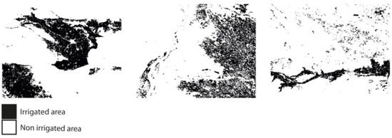
Figure 6.
Irrigated area of 2016 derived from PROBA-V data at 10 arc seconds (approx. 300 m) for the regions of China (left), Sudan (middle) and USA (right).
Table 2.
Comparison of the irrigation mapping results using PROBA-V and the degraded Sentinel-2 data at 300 m.
We thus conclude that our irrigation mapping method using annual NDVI courses is transferable between Sentinel-2 and PROBA-V data. On the other hand, our analysis of the mapping results at different spatial resolutions shows that Sentinel-2, at a resolution of 10m, is able to detect additional irrigated areas which are lost at the coarser resolution. On the other hand, the large data volume involved would be a large obstacle for an operational global irrigation monitoring system based on Sentinel-2. By possibly using scaling relations that would, depending on the geographical setting, allow us to correct for the lost irrigated area in the coarse resolution operational irrigation monitoring system, the use of 10m-resolution Sentinel-2 data would largely enhance the monitoring result. Here, we propose a framework which would allow global PROBA-V irrigation monitoring to profit from sample Sentinel-2 irrigation mapping by allying appropriate scaling relations.
3.3. Scaling Relation between Lost Irrigated Area and the Landscape Shape Index
In Section 2.2, we hypothesized a relationship between the Landscape Shape Index and the negative areal change of the irrigation mapping with spatial resolution. When applying the LSI to the 36 sub-tiles in each of the three selected Sentinel-2 tiles, the results in Figure 7 show a strong linear relationship between the LSI and the negative change of the mapped irrigation area at 300 m compared to at 10 m (Sudan: r = −0.92, USA: r = −0.95, China: r = −0.96). Figure 7 shows the result in the three regions and the different characterization of the areal change and the LSI.
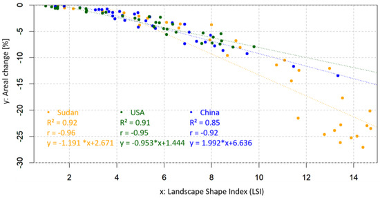
Figure 7.
Loss of the mapped irrigated area from 10 m to 300 m spatial resolution as a function of the Landscape Shape Index (LSI) in the three regions: Sudan, USA and China.
At small values, the relationship in all three regions behave similarly. Higher LSI values are observed in Sudan and changes the linear equation compared to the equations in USA and China. This shows that the mapping result depends on the spatial formation and arrangement and the complexity of the shape of the irrigation network. These relations seem to be independent from the region and are based solely on the spatial arrangement and the complexity of the shapes of the mapped irrigated area.
4. Discussion
This study represents a systematical analysis of the influence of spatial resolution of the selected sensor on the mapped irrigated area. The study confirms the findings of Velpuri et al. [24], in that the mapped irrigated area generally decreases when moving to a coarser spatial resolution. The magnitude of change in the irrigated area with spatial resolution shows a strong linear relation with the LSI in all three regions and seems to be regionally independent.
However, many factors influence the scaling relation, with the characteristics of the regional farming system being the most obvious. These characteristic farming systems result in the spatial formation of the irrigated fields and were affected differently according to their shape and their spatial arrangement in the coarser spatial resolution. While the mapping result in China stayed constant, the analyzed regions in Sudan and USA showed large discrepancies in the mapped irrigated area at different spatial resolutions. This implies a high complexity of the irrigation patterns which affect the spectral upscaling to a coarser resolution, while the irrigated area in China is ordered mainly in irrigation agglomerations with a low complexity in shape. That means the determination of irrigated areas in regions of small and scattered fields is more affected when moving to coarser resolutions than in regions of larger, connected fields in areas which are completely used for agriculture. As soon as single fields are embedded in a non-irrigated surrounding of fallow fields or barren land, the identified irrigated area is highly sensitive to a decrease in resolutions.
The upscaling of the spectral information smooths the NDVI signal and influences the mapping method. This leads to a significant change of the average NDVI in case of a high NDVI variation at the underlying resolution. High NDVI variations are caused by different growth phase or by a mix of different land uses at one 300 m-resolution pixel. This effect is shown in the example of Sudan, where the landscape is characterized by a mix of small fields, meadows and settlements interrupted by streets and fallow land. At coarser resolutions (>100 m), this leads to high variations in the NDVI within one coarse resolution pixel and, thereby, influences the mapping result (Figure 3 and Figure 5).
The largest absolute changes in identified irrigated area with decreasing spatial resolutions were found in the USA. The differences may have several reasons: The annual precipitation in the region is 329 mm/a, which is the highest of the three compared regions. For rain-fed agricultural systems, this precipitation amount is very low, causing supplemental irrigation systems to be widely used in this area. Precipitation events might occur very locally and in summer as heavy thunderstorms, which have comparable effects to technical irrigation. The high-resolution images show small water ponds and water channels used for storage and transportation of water from wells or water bodies to the irrigated fields. The greening effect around the water storage and transportation bodies are part of the high-resolution images but are too small to be resolved in the coarser resolution images. Decreasing the resolution, therefore, affects the recognition of the areas around the water bodies and results in a smaller irrigated area. The most decisive reason is the structure and the complexity of shape of the agricultural fields in this area. The irrigated fields in the north of the scene are distributed spatially, separated by barren land, pastures or unmanaged land. This leads to low NDVI values at the coarser resolutions, which reduce the identified irrigated area. However, the NDVI is limited regarding the fast saturation in case of active vegetation and does not provide details about biomass or LAI [41]. The example in the USA shows the difficulties of greening along water-channels or the greening after small-scale precipitation events, which leads to higher NDVI-values and influences the irrigation mapping method. In contrast to the results in the USA and Sudan, the mapping results in China are very similar at all spatial resolutions. Large-scaled fields of similar sizes and a small share of fallow fields characterize the two large agricultural areas of the scene. They indicate that the farming system follows a central management scheme resulting in a low complexity of the shape of the fields. The regular pattern of the fields, the absence of fallow fields and the large size of the fields in combination result in constant NDVI values across the different spatial resolutions and, hence, scale-independent mapping results.
Besides the different behavior regarding the mapping result at a coarser spatial resolution in China compared to Sudan and the USA, the relation of the negative changes of mapped irrigated area and the LSI behaves in all three regions constantly. This means the negative areal change of irrigated area with resolution is explained by the LSI and shows that landscape metrics can also be used outside of the analysis of natural ecosystems in man-made patterns. The relations between negative areal change and LSI can be used as information about the considered region regarding an expected loss of mapped irrigated area at a coarser resolution derived by wide-swath medium-resolution satellites. A transferability is possible, since the study showed that the downscaled Sentinel-2 and original PROBA-V NDVI time series of the same spatial resolution and the same time period were practically identical despite the differences in sensor characteristics, measurement and sun angle. This demonstrates the stability of the overall approach and allows to link Sentinel-2- and PROBA-V-derived irrigation maps. The scaling relation builds a bridge between the medium-resolution sensors such as PROBA-V or the new Sentinel-3 mission and high-resolution sensors such as Sentinel-2.
The presented results identify three main driving forces on the extent of the irrigated area: (a) the spatial resolution, (b) the spatial distribution of the irrigated fields in the analyzed area and (c) the complexity of the shape of the connected irrigated fields. Changes in the spatial resolution influence the mapping results differently depending on the spatial distribution and the complexity of the shape of the irrigated fields in the analyzed area. Thus, the influence of the spatial resolution on the mapping results differs from landscape to landscape. The trend towards spatially and temporally high-resolution satellite data and high-performance computing offers opportunities to rethink existing methods of irrigation mapping considering local conditions such as the spatial distribution of fields and combine crop growth model results with derived information about the development of biomass and plant conditions.
5. Conclusions
Overall, it can be concluded that the mapping of irrigated area using an NDVI threshold approach highly depends on both the spatial distribution of irrigated fields and the spatial resolution of the observing sensor. The study demonstrates the potential of Sentinel-2 to open a new chapter of irrigation mapping by providing high-spatial-resolution NDVI time series with a temporal resolution of up to 2.5 days and can be applied as a transition from the historical irrigation mapping with wide-swath medium-resolution sensors such as VEGETATION, MODIS and AVHRR to an irrigation monitoring at a high temporal and spatial resolution. Further, the use of the landscape metrics shows the potential to estimate an expected accuracy of irrigation mapping derived by wide-swath medium-resolution satellites such as Sentinel-3. Landscape metrics can identify regions characterized by a high expected loss in irrigation mapping with coarser resolution. The information about the influence of spatial scale on irrigation mapping will increase the accuracy of the estimation of the actual amount of water that is withdrawn from the regional water resources and diverted regionally into the atmosphere by irrigation.
The next step should be the development of an automatically updated irrigation monitoring system which supplies the users up-to-date information about the state of irrigation in terms of location, area and type. Irrigation monitoring as input information in spatially distributed crop growth models will improve the model results regarding water flows. The comparison of the model results with time series of multispectral remote sensing observations, which document the development of the irrigated crops from seeding to harvest, will allow the traceability of irrigation management such as the used irrigation water by the crops, irrigation water loss through interception or soil evaporation and overall water use efficiency. A remote-sensing-based monitoring system of the described kind is the prerequisite for the improvement of irrigation management towards a less wasteful use of the precious water resources by the farmers and can be a strong instrument in negotiations regarding upstream–downstream water conflicts in large watersheds.
Author Contributions
Conceptualization, J.M. and W.M.; methodology, J.M. and W.M.; software, J.M.; formal analysis, J.M. and W.M.; data curation, J.M.; writing—original draft preparation, J.M.; writing—review and editing, J.M. and W.M.; visualization, J.M.; supervision, W.M. All authors have read and agreed to the published version of the manuscript.
Funding
This research was funded by the Bavarian Environment Agency (Landesamt für Umwelt, LfU) under the grant number 81-44214.9-89131/2017, 81-4421.9-89123/2017 and 81-4421.992819/2017, by the open access publication fund of the German Aerospace Center (DLR) and to a smaller part by AgRAIN, a project funded by the Federal Ministry of Education and Research (Bundesministerium für Bildung und Forschung, BMBF) under the grant number 01LZ1904A.
Data Availability Statement
The irrigation maps at different spatial scale produced in this study are available from the corresponding author upon reasonable request.
Acknowledgments
The authors would like to thank the Vista GmbH—Remote Sensing Applications in Geosciences for providing the processed Sentinel-2 data. We also gratefully acknowledge the anonymous reviewers and editors for constructive comments for improvement of the manuscript. The responsibility for the content of this publication lies with the authors.
Conflicts of Interest
The authors declare no conflict of interest. The funders had no role in the design of the study; in the collection, analyses or interpretation of data; in the writing of the manuscript, or in the decision to publish the results.
References
- Mueller, N.D.; Gerber, J.S.; Johnston, M.; Ray, D.K.; Ramankutty, N.; Foley, J.A. Closing yield gaps through nutrient and water management. Nature 2012, 490, 254–257. [Google Scholar] [CrossRef]
- Foley, J.A.; Ramankutty, N.; Brauman, K.A.; Cassidy, E.S.; Gerber, J.S.; Johnston, M.; Mueller, N.D.; O’Connell, C.; Ray, D.K.; West, P.C.; et al. Solutions for a cultivated planet. Nature 2011, 478, 337–342. [Google Scholar] [CrossRef]
- FAO. FAOSTAT; Food and Agriculture Organization of the United Nations (FAO): Paris, France, 2016. [Google Scholar]
- FAO. Total Withdrawal by Sector; Food and Agriculture Organization of the United Nations (FAO): Paris, France, 2014. [Google Scholar]
- Neumann, K.; Stehfest, E.; Verburg, P.H.; Siebert, S.; Müller, C.; Veldkamp, T. Exploring global irrigation patterns: A multilevel modelling approach. Agric. Syst. 2011, 104, 703–713. [Google Scholar] [CrossRef]
- Puy, A. Irrigated areas grow faster than the population. Ecol. Appl. 2018, 28, 1413–1419. [Google Scholar] [CrossRef] [PubMed]
- Meier, J.; Zabel, F.; Mauser, W. A global approach to estimate irrigated areas—A comparison between different data and statistics. Hydrol. Earth Syst. Sci. 2018, 22, 1119–1133. [Google Scholar] [CrossRef]
- Strzepek, K.; Boehlert, B. Competition for water for the food system. Philos. Trans. R. Soc. London. Ser. B Biol. Sci. 2010, 365, 2927–2940. [Google Scholar] [CrossRef] [PubMed]
- Micklin, P. The Aral Sea Disaster. Annu. Rev. Earth Planet. Sci. 2007, 35, 47–72. [Google Scholar] [CrossRef]
- Chen, L.; Ma, Z.-G.; Zhao, T.-B.; Li, Z.-H.; Li, Y.-P. Simulation of the regional climatic effect of irrigation over the Yellow River Basin. Atmos. Ocean. Sci. Lett. 2017, 10, 291–297. [Google Scholar] [CrossRef]
- Udall, B.; Overpeck, J. The twenty-first century Colorado River hot drought and implications for the future. Water Resour. Res. 2017, 53, 2404–2418. [Google Scholar] [CrossRef]
- Maupin, M.A.; Ivahnenko, T.; Bruce, B. Estimates of Water Use and Trends in the Colorado River Basin, Southwestern United States, 1985–2010. In U.S. Geological Survey Scientific Investigations Report 2018-5049; U.S. Geological Survey: Reston, VA, USA, 2018. [Google Scholar]
- Ozdogan, M.; Yang, Y.; Allez, G.; Cervantes, C. Remote Sensing of Irrigated Agriculture: Opportunities and Challenges. Remote Sens. 2010, 2, 2274–2304. [Google Scholar] [CrossRef]
- Ozdogan, M.; Gutman, G. A new methodology to map irrigated areas using multi-temporal MODIS and ancillary data: An application example in the continental US. Remote Sens. Environ. 2008, 112, 3520–3537. [Google Scholar] [CrossRef]
- Ambika, A.K.; Wardlow, B.; Mishra, V. Remotely sensed high resolution irrigated area mapping in India for 2000 to 2015. Sci. Data 2016, 3, 160118. [Google Scholar] [CrossRef]
- Jin, N.; Tao, B.; Ren, W.; Feng, M.; Sun, R.; He, L.; Zhuang, W.; Yu, Q. Mapping Irrigated and Rainfed Wheat Areas Using Multi-Temporal Satellite Data. Remote Sens. 2016, 8, 207. [Google Scholar] [CrossRef]
- Salmon, J.M.; Friedl, M.A.; Frolking, S.; Wisser, D.; Douglas, E.M. Global rain-fed, irrigated, and paddy croplands: A new high resolution map derived from remote sensing, crop inventories and climate data. Int. J. Appl. Earth Obs. Geoinf. 2015, 38, 321–334. [Google Scholar] [CrossRef]
- Thenkabail, P.S.; Biradar, C.M.; Noojipady, P.; Dheeravath, V.; Li, Y.; Velpuri, M.; Gumma, M.; Gangalakunta, O.R.P.; Turral, H.; Cai, X.; et al. Global irrigated area map (GIAM), derived from remote sensing, for the end of the last millennium. Int. J. Remote Sens. 2009, 30, 3679–3733. [Google Scholar] [CrossRef]
- Cammalleri, C.; Anderson, M.C.; Gao, F.; Hain, C.R.; Kustas, W.P. Mapping daily evapotranspiration at field scales over rainfed and irrigated agricultural areas using remote sensing data fusion. Agric. For. Meteorol. 2014, 186, 1–11. [Google Scholar] [CrossRef]
- Abuzar, M.; McAllister, A.; Whitfield, D. Mapping Irrigated Farmlands Using Vegetation and Thermal Thresholds Derived from Landsat and ASTER Data in an Irrigation District of Australia. Photogramm. Eng. Remote Sens. 2015, 81, 229–238. [Google Scholar]
- Lawston, P.M.; Santanello, J.A.; Kumar, S.V. Irrigation Signals Detected From SMAP Soil Moisture Retrievals. Geophys. Res. Lett. 2017, 44, 860–867. [Google Scholar] [CrossRef]
- Puy, A.; Sheikholeslami, R.; Gupta, H.V.; Hall, J.W.; Lankford, B.; Lo Piano, S.; Meier, J.; Pappenberger, F.; Porporato, A.; Vico, G.; et al. The delusive accuracy of global irrigation water withdrawal estimates. Nat. Commun. 2022, 13, 3183. [Google Scholar] [CrossRef]
- Puy, A.; Lankford, B.; Meier, J.; van der Kooij, S.; Saltelli, A. Large variations in global irrigation withdrawals caused by uncertain irrigation efficiencies. Environ. Res. Lett. 2022, 17, 044014. [Google Scholar] [CrossRef]
- Velpuri, N.M.; Thenkabail, P.S.; Gumma, M.K.; Biradar, C.; Dheeravath, V.; Noojipady, P.; Yuanjie, L. Influence of Resolution in Irrigated Area Mapping and Area Estimation. Photogramm. Eng. Remote Sens. 2009, 75, 1383–1395. [Google Scholar] [CrossRef]
- Ferrant, S.; Selles, A.; Le Page, M.; Herrault, P.-A.; Pelletier, C.; Al-Bitar, A.; Mermoz, S.; Gascoin, S.; Bouvet, A.; Saqalli, M.; et al. Detection of Irrigated Crops from Sentinel-1 and Sentinel-2 Data to Estimate Seasonal Groundwater Use in South India. Remote Sens. 2017, 9, 1119. [Google Scholar] [CrossRef]
- Sharma, A.K.; Hubert-Moy, L.; Buvaneshwari, S.; Sekhar, M.; Ruiz, L.; Bandyopadhyay, S.; Corgne, S. Irrigation History Estimation Using Multitemporal Landsat Satellite Images: Application to an Intensive Groundwater Irrigated Agricultural Watershed in India. Remote Sens. 2018, 10, 893. [Google Scholar] [CrossRef]
- Demarez, V.; Helen, F.; Marais-Sicre, C.; Baup, F. In-Season Mapping of Irrigated Crops Using Landsat 8 and Sentinel-1 Time Series. Remote Sens. 2019, 11, 118. [Google Scholar] [CrossRef]
- Patton, D.R. A Diversity Index for Quantifying Habitat “Edge”. Wildl. Soc. Bull. 1975, 3, 171–173. [Google Scholar]
- Hargis, C.D.; Bissonette, J.A.; David, J.L. The behavior of landscape metrics commonly used in the study of habitat fragmentation. Landsc. Ecol. 1998, 13, 167–186. [Google Scholar] [CrossRef]
- Bogaert, J.; Van Hecke, P.; Salvador-Van Eysenrode, D.; Impens, I. Quantifying habitat edge for nature reserve design. Coenoses 1998, 13, 131–136. [Google Scholar]
- Wang, X.; Blanchet, F.G.; Koper, N.; Tatem, A. Measuring habitat fragmentation: An evaluation of landscape pattern metrics. Methods Ecol. Evol. 2014, 5, 634–646. [Google Scholar] [CrossRef]
- Nowosad, J.; Stepinski, T.F. Information theory as a consistent framework for quantification and classification of landscape patterns. Landsc. Ecol. 2019, 34, 2091–2101. [Google Scholar] [CrossRef]
- Zabel, F.; Putzenlechner, B.; Mauser, W. Global agricultural land resources—A high resolution suitability evaluation and its perspectives until 2100 under climate change conditions. PLoS ONE 2014, 9, e107522. [Google Scholar] [CrossRef]
- Hersbach, H.; Bell, B.; Berrisford, P.; Hirahara, S.; Horányi, A.; Muñoz-Sabater, J.; Nicolas, J.; Peubey, C.; Radu, R.; Schepers, D.; et al. The ERA5 global reanalysis. Q. J. R. Meteorol. Soc. 2020, 146, 1999–2049. [Google Scholar] [CrossRef]
- Fritz, S.; See, L.; McCallum, I.; You, L.; Bun, A.; Moltchanova, E.; Duerauer, M.; Albrecht, F.; Schill, C.; Perger, C.; et al. Mapping global cropland and field size. Glob. Chang. Biol. 2015, 21, 1980–1992. [Google Scholar] [CrossRef] [PubMed]
- Monfreda, C.; Ramankutty, N.; Foley, J. Farming the planet: 2. Geographic distribution of crop areas, yields, physiological types, and net primary production in the year 2000. Glob. Biogeochem. Cycles 2008, 22. [Google Scholar] [CrossRef]
- Sterckx, S.; Benhadj, I.; Duhoux, G.; Livens, S.; Dierckx, W.; Goor, E.; Adriaensen, S.; Heyns, W.; Van Hoof, K.; Strackx, G.; et al. The PROBA-V mission: Image processing and calibration. Int. J. Remote Sens. 2014, 35, 2565–2588. [Google Scholar] [CrossRef]
- Santandrea, S.; Mellab, K.; Vrancken, D.; Versluys, J. The PROBA-V mission: The space segment AU—Francois, Michael. Int. J. Remote Sens. 2014, 35, 2548–2564. [Google Scholar] [CrossRef]
- Verhoef, W.; Bach, H. Simulation of hyperspectral and directional radiance images using coupled biophysical and atmospheric radiative transfer models. Remote Sens. Environ. 2003, 87, 23–41. [Google Scholar] [CrossRef]
- Hesselbarth, M.H.K.; Sciaini, M.; With, K.A.; Wiegand, K.; Nowosad, J. landscapemetrics: An open-source R tool to calculate landscape metrics. Ecography 2019, 42, 1648–1657. [Google Scholar] [CrossRef]
- Viña, A.; Gitelson, A.A.; Nguy-Robertson, A.L.; Peng, Y. Comparison of different vegetation indices for the remote assessment of green leaf area index of crops. Remote Sens. Environ. 2011, 115, 3468–3478. [Google Scholar] [CrossRef]
Disclaimer/Publisher’s Note: The statements, opinions and data contained in all publications are solely those of the individual author(s) and contributor(s) and not of MDPI and/or the editor(s). MDPI and/or the editor(s) disclaim responsibility for any injury to people or property resulting from any ideas, methods, instructions or products referred to in the content. |
© 2023 by the authors. Licensee MDPI, Basel, Switzerland. This article is an open access article distributed under the terms and conditions of the Creative Commons Attribution (CC BY) license (https://creativecommons.org/licenses/by/4.0/).