SAR Image Classification Using Gated Channel Attention Based Convolutional Neural Network

Abstract

Algorithms combining CNN (Convolutional Neural Network) and super-pixel based smoothing have been proposed in recent years for Synthetic Aperture Radar (SAR) image classification. However, the smoothing may lead to the damage of details. To solve this problem the feature fusion strategy is utilized, and a novel adaptive fusion module named Gated Channel Attention (GCA) is designed in this paper. In this module, the relevance between channels is embedded into the conventional gated attention module to emphasize the variation in contribution on classification results between channels of feature-maps, which is not well considered by the conventional gated attention module. A GCA-CNN network is then constructed for SAR image classification. In this network, feature-maps corresponding to the original image and the smoothed image are extracted, respectively, by feature-extraction layers and adaptively fused. The fused features are used to obtain the results. Classification can be performed by the GCA-CNN in an end-to-end way. By the adaptive feature fusion in GCA-CNN, the smoothing of misclassification and the detail keeping can be realized at the same time. Experiments have been performed on one elaborately designed synthetic image and three real world SAR images. The superiority of the GCA-CNN is demonstrated by comparing with the conventional algorithms and the relative state-of-the-art algorithms.

1. Introduction

The Synthetic Aperture Radar (SAR) can work under all time and all weather conditions with relatively higher resolution. Due to the advantage above, the SAR images have been widely applied to sea ice detection, terrain surface classification, mapping, agriculture monitoring, and military applications. Consequently, the interpretation of SAR images with high accuracy and efficiency is important. As the fundamental step of SAR image processing, SAR image classification is a hot topic in remote sensing.

Feature extraction is the most crucial step in the SAR image classification. The CNN can extract robust and representative image features using multiple convolution kernels in the convolution layers in an automatic way [1,2,3,4]. Consequently, in recent years the CNN has been constantly and successfully used for SAR image classification [5,6,7,8,9,10,11,12,13,14,15,16,17]. A Variety of CNN-based SAR image classification algorithms have been proposed, and obvious improvements in classification accuracy have been achieved.

However, the intrinsic spatial neighborhood information of SAR images cannot be explored by the conventional CNN framework. To utilize the intrinsic spatial neighborhood information to improve the classification accuracy in future, some algorithms combining the CNN and the super-pixels were proposed. Duan et al. [8] performed the super-pixel based smoothing by using the voting strategy after the classification using CNN. Hou et al. [9] employed the deep learning method to obtain the labels of pixels and utilized the k-nearest neighborhood method to obtain the labels of sup-pixels. Liu et al. [10] performed the super-pixel based classification on the input SAR image to reduce the impact of speckle noise. Following these works, we also proposed a super-pixel oriented SAR image classification algorithm based the CNN [12]. In our work, the overall accuracy is obviously enhanced because of the elimination of misclassification using spatial neighborhood information. However, some details in the narrow regions, especially the locating of boundaries, are destroyed.

Feature fusion could be considered as a reasonable strategy to improve the detail-keeping capability of the CNN and super-pixel based classification algorithms, where the features of the smoothed homogeneous regions and the features of details can be fused. For the existing SAR image classification algorithms, concatenating the features [13] and averaging the features [14] are the two commonly used ways for the feature fusion. However, the contributions of the features to be fused on the classification result are not considered. To emphasize the contributions of features, a gated heterogeneous fusion module was proposed by Li et al. [15] to perform the adaptive fusion of two groups of feature-maps. In this module, the two groups of feature-maps are used to produce the corresponding gated coefficient (denoted as G and 1-G) for adaptive fusion. Based on Li’s work, this paper suggests that the gated mechanism can also be regarded as a kind of binary attention module which emphasizes the importance of two groups of feature-maps. However, in the conventional Gated Attention (GA) module the variation in contribution on classification between channels of feature-maps is not well considered, which may limit performance of adaptive feature fusion. As indicated by Liang et al. [14], the variation in contribution between channels of feature-maps can be described by utilizing the relevance between channels.

The channel attention mechanism is recently utilized in the SAR image classification to describe the relevance between channels of feature-maps [18]. Inspired by the channel attention mechanism, a new attention module called Gated Channel Attention (GCA) module, which embeds the channel relevance description into the conventional Gated Attention (GA) module, is proposed for the adaptive feature fusion in this paper. In the GCA module, the adaptive gated channel attention coefficients are obtained by utilizing the global pooling and a fully connected sub-network. According to the gated channel attention coefficients, adaptive feature fusion is then conducted using a gated mechanism. In this way, the relevance between channels can be described by the weights in the fully connected sub-network, and the difference in importance on classification feature-maps can then be considered by the gated mechanism. Based on the GCA module, a new SAR image classification network, which is called GCA-CNN, is proposed. Before the GCA-CNN, an adaptive intrinsic neighborhood weighted based smoothing technique, which considers the details keeping, is developed to obtain the smoothed image. In the GCA-CNN, a two-branch feature-extraction module is used to obtain representative image features of the original and smoothed SAR images. Two groups of feature-maps are generated by the feature extraction module and adaptively fused by GCA. The fused feature-maps are finally put into the classification module to perform the classification. The parameters in the GCA module can be automatically adjusted. By utilizing the proposed GCA-CNN framework, the smoothing of misclassification and the detail keeping, especially in the narrow regions, can be realized at the same time. Experiments were performed using a synthetic SAR image and two real world Radarsat-2 SAR images. The effectiveness of the proposed algorithm can be demonstrated by the results of experiments.

In summary, the novelty of the proposed algorithm derives from the following points. The points (1) and (2) are the technical innovation of this paper, while point (3) is the practical innovation:

(1)

An adaptive intrinsic neighborhood weighted based smoothing technique is developed in this paper, in which the counter-balance between smoothing and details keeping is considered;

(2)

From the aspect of attention mechanism, the relevance between channels of feature-maps is embedded into the conventional GA module to construct a new kind of feature fusion module called Gated Channel Attention (GCA) module. The fusion performance can be improved comparing the GA by considering the difference in contribution on classification between channels of feature-maps more adequately;

(3)

Based on the GCA module, a new Convolution Neural Network called GCA-CNN is constructed. Parameters in the GCA module and the other parts of GCA-CNN can be simultaneously adjusted. Keeping the details and reducing the misclassification can be realized by utilizing the proposed GCA-CNN.

2. Background and Related Works

2.1. Convolutional Neural Network

CNN is a widely used framework of the deep artificial neural network in the field of image classification. The primary framework of CNN, which is called LeNet-5, was proposed by Lecun in 1998 [19], and was successfully used in handwriting recognition. In the 2012 [1] a new network with larger depth called AlexNet was proposed. In the framework of AlexNet, a new nonlinear active function called ReLU (Rectified Linear Unit) [20] was applied to increase the sparsity of the convolution layers. To process the features with multi-scales, the GoogleNet [3] was proposed by Szegedy et al. The GoogleNet is composed of Inception modules which consist of branches with different scales of convolutional kernels. Due to the elaborately designed structure, the GoogleNet can process the multi-scale features well. The ResNet [2] was proposed by back-propagating the error of higher layers directly to lower layers while the intermediate layers are skipped, which can deal with the problem of gradient vanishing. To emphasize the significance of each channel, the SENet [18] in which the global pooling results of each channel are used to obtain the weights for all the channels by an adaptive way was proposed. Although a series of advanced CNN frameworks were proposed, the LeNet-5 can still act as the backbone of CNN. The structure of LeNet-5 is demonstrated in Figure 1. The CNN shown in Figure 1 contains two groups of convolution-pooling layers, a fully connected layer and a softmax classifier.

The convolution layers are constructed to obtain muti-features from the input feature-maps by using operation of convolution, which can be quantified expressed as:

$${\mathrm{y}}_{\mathrm{i}}^{\mathrm{l}}=\mathrm{Re}LU({\displaystyle \sum _{i=1}^m{x}_i^{l-1}\times w_{ji}^l+b_j^l})$$

(1)

where y and x refer to the output and the input, l refers the l^th layer, while i and j denote the i^th and j^th feature maps. The w refers to weights connecting the l^th layer and the l−1^th layer, and $b_j^l$ represents the bias in the l^th layer. ReLU() refers to the Linear rectification function.

The feature-maps obtained by the operation of convolution layer are then processed by the pooling layer. Usually, in the pooling layer, an m × m patch is sub-sampled as a certain value. The max-pooling and average-pooling, which output the maximum or minimum values of image patches, are usually utilized. The functionality of the pooling layers comes from three folds: the reduction in data size, the enlarging of receptive field, and the reducing of noise.

After the convolution and pooling layers, there are the fully connected layers where the local features are stretched and integrated as a global feature-vector. The feature-vector might be processed by the following layers or put into the softmax classifier.

2.2. Attention Mechanism

Attention mechanism was firstly proposed for the machine translation, which is used to emphasize the importance of words in the sentences to be translated.

In recent years, the study of attention mechanism has been one of the hot topics in the deep learning. Attention mechanism originates from the thought of bionics and is an imitation of human attention mechanism. For example, human visual attention usually focuses on important information that helps to distinguish and ignores irrelevant information. In the investigation of computer vision, the mechanism of attention is used to emphasize the importance of channel and spatial locations to reduce feature redundancy and improve discrimination of image features.

Attention mechanism has been successfully utilized in the processing of the remote sensing images. At present, in the field of remote sensing image classification, attention mechanism can be widely divided as the spatial attention, the channel attention and the spatial-channel hybrid attention. Wang et al. [21] used the spatial attention in the last feature-map of CNN to improve the global representation capability of the CNN model. The performance of this algorithm is obviously improved compared with conventional algorithms. Tong et al. combined [22] channel attention with the DenseNet model and proposed a new DenseNet model which is then used for remote sensing image scenes classification. Based on the work of Tong, Zhao et al. [23] proposed a hybrid attention module called EAM (enhanced attention module) and applied it to the ResNet model. The experimental results indicate that the hybrid attention module is more useful to the improvement in the classification accuracy. Based on the work of Zhao, Mei et al. [24] used the recurrent neural network to generate a channel attention coefficient to describe the correlation between channels. The recurrent neural network was originally used to process time series and can describe the correlation of input at adjacent time points. In order to realize the adaptive generation of the channel and spatial attention coefficient, Yu et al. [25] proposed the feeding-back based attention module, which optimizes the attention coefficients through the back-propagation of training error and improves the coupling between the attention module and the classification network. The attention mechanism is also applied to the Graph Convolutional Network (GCN). In the work of Ma et al. [26], the attention mechanism was used before the first graph convolution layer to describe the correlations between the graph nodes. The GCN with attention was then used to perform the region-level SAR image classification. As discussed above, the attention mechanism has been widely used in the field of remote sensing and SAR image classification to emphasize the importance of pixels and channels on classification. Inspired by the functionality of the attention module, the idea of attention is proposed to be utilized for the feature fusion. Based on this idea, the gated module can also be regarded as a binary attention module. This binary attention module can adaptively emphasize the contributions of two groups of feature maps on the classification. However, in this gated attention module the variation in contribution on classification between channels of feature-maps is not well considered. As each channel of feature maps contains unique features, the contribution of channels on classification are different from each other. To address this problem, the relevance between channels is embedded into the conventional gated attention mechanism to form a new attention module which emphasizes the difference in contribution between channels.

3. Proposed Method

In this paper, a novel neural network named GCA-CNN is proposed for the SAR image classification, in which the smoothing of misclassification and the keeping of details can be realized at the same time by adaptive feature fusion. The adaptive fusion is realized by the GCA module which is newly proposed in this paper. The GCA module is constructed by combining the GA mechanism and the channel attention mechanism. In the GCA, the relevance between channels is embedded into the conventional GA module to emphasize the variation in contribution between channels, which is caused by the difference in features between feature-maps. By exploring the GCA module, the fusion performance can be improved comparing with GA. In the process of SAR image classification, feature-maps corresponding to the super-pixel based smoothed image and original image are extracted using the front layers, and these feature-maps will be adaptively fused, channel by channel, according to the kind of region to be classified. The fused features are finally fed into the last classification layer to obtain the results. In this way, the features corresponding to the details are highlighted when classifying the narrow regions, while the features corresponding to the smoothed image are highlighted when classifying the homogeneous regions. Note that the GCA module is integrated into the CNN framework while the parameters in the GCA module and the layers are adjusted simultaneously. Updating formulas of parameters in the GCA-CNN, especially in the GCA module, is developed in this paper. The superiority of the proposed GCA-CNN is experimentally proven in Section 4.

The workflow of the proposed algorithm Is shown in Figure 2. In Section 3.1, the super-pixel based smoothing is introduced as the preprocessing of SAR images. In Section 3.2, the structure and function of a dual-branch feature extraction module are illustrated. In Section 3.3, the mechanism of the GCA module is explained in detail. In Section 3.4, the classification module and the training strategy of the GCA-CNN network, especially for the GCA, is presented.

3.1. The Super-Pixel and Adaptive Neighborhood Weighting Based Smoothing

To take advantage of the spatial correlation within the intrinsic SAR image neighborhood to improve the overall accuracy especially for the homogeneous regions, a super-pixel and adaptive neighborhood weighting-based smoothing method is proposed and implemented in this paper. In the first step, the SLIC (Simple Linear Iterative Clustering) algorithm [27] is applied to generate the super-pixels.

After the generation of super-pixels, an adaptive neighborhood weighting based on smoothing the interior the sup-pixels is implemented. In this step, for a pixel I which belongs to super-pixel S_k, the intensity of i is replaced by the adaptive weighted average of the intensities of neighborhood pixels (within the same super-pixel S_k) of pixel i. This step can be illustrated as Equation (2):

$${\overline{I}}_{\mathrm{i}}=\beta I_i+(1-\beta ){\displaystyle \sum _{p_i\in S_k}{w}_{ij}{I}_j}$$

(2)

where $I_i$ is the original intensity of pixel i, and j corresponds to the pixel j located within the same sup-pixel. The coefficient of $I_i$ is $\beta$, which is a value between 0 and 1. Exploring the original intensity of pixel i is to prevent the over-smoothing of the SAR image. The ${\displaystyle \sum {\mathrm{w}}_{ij}{I}_j}$ is the weighted average of the intensities of pixels within the same sup-pixel and the corresponding coefficient is $1-\beta$. The adaptive weight corresponding to a neighborhood pixel is calculated according to the intensity distance between a pair of pixels. Taking pixel i and j as an example, which is shown in Equation (3):

$$w_{ij}=\mathit{exp}(-\frac{|I_i-I_j|}{{\sigma }^2})$$

(3)

where exp() represents the exponent function, |$I_i-I_j$| is the absolute value of intensity difference between pixel i and j, ${\sigma }^2$ refers to the variance of the intensity values of pixels within the super-pixel.

3.2. The Dual-Branch Feature Extraction Module

After the super-pixel based smoothing, the feature extraction module with dual-branches, which takes the CNN as the backbone, is designed for the feature extraction of the original image and smoothed image, respectively. In this step, the CNN is applied as the backbone of the dual-branch feature extraction module. The structure of the dual-branches module is shown in the left part of Figure 3.

As given in Figure 3, the upper branch and the lower branch share the same structure, which is experimentally determined. However, the convolution kernels and biases of these two branches are different. Consequently, the two branches are given in different colors. The original image and the smoothed image are put into the feature extraction module for feature extraction according to Equation (4):

$$F{M}_1=F_{{\mathrm{branch}}_1}(I_{\mathrm{original}},{\theta }_1);F{M}_2=F_{{\mathrm{branch}}_2}(I_{\mathrm{smoothed}},{\theta }_2)$$

(4)

In Equation (4), FM₁ and FM₂ correspond to the feature-maps extracted by the first and second branch, respectively, and θ₁ and θ₂ are the parameters of the first and second CNN branch. After this step, the extracted deep feature denoted as FM₁ and FM₂ will be adaptively fused by the GCA module according to the importance on classification results.

3.3. The GCA Module

The structure of the GCA module is illustrated in the middle part of Figure 3. The GCA module consists of an input layer, a global pooling layer, two fully connected layers to generate the channel attention coefficient, and a fusing layer constructed based on the gated mechanism. The input layer is explored to receive the feature-maps corresponding to the original image (denoted as FM₁), and the feature-maps correspond to the smoothed image (denoted as FM₂) as the input of the GCA. In the global pooling layer the operation of global pooling is utilized on each channel of FM₁ and the FM₂. After the global pooling, for each channel of the feature-maps a specific value is obtained to represent this channel.

As a result, a feature-vector is generated to represent a group of feature-maps, which is described by Equation (5):

$$[f_1,f_2,\dots ,f_n]=globalpooling(C_1,C_2,\dots ,C_n)$$

(5)

where C_i represents channel i and f_i is the corresponding feature obtained by global-pooling. By implementing the global pooling on the two groups of feature maps, two feature vectors with the same dimension are produced. These two feature vectors are then concatenated into a new feature vector which is taken as the input of the fully connected layers for generating the attention coefficient.

The fully connected layers are used to produce the gated channel attention coefficients. The form of the multi-layer perceptron is taken as the backbone to construct the fully connected layers. In the fully connected structure, the relevance of the channels can be described by the weights of the channels. The ReLU (Rectified Linear Units) function is applied as the active function of the first fully connected layer to make the parameters of the GCA module sparser. The expression of the operating of this layer is written as:

$$y_i=ReLU(w_i^{T}f+b_i)$$

(6)

In Equation (6), f represents the input feature vector, $w_i^T$ refers to the weight of the i^th neuron unit in the first layer, while b_i means the bias of the same neuron unit. For the second fully connected layer, the widely used sigmoid function is utilized to refine the output values which represent the gated attention coefficient into (0,1). The operation of the second layer is described as:

$${\lambda }_i=sigm(w_{(2)i}^{T}f+b_{(2)i})$$

(7)

In Equation (7), $w_{(2)i}^T$ refers to the weight of the i^th neuron unit in the second layer and $b_{(2)i}^T$ refers to the corresponding bias. After the nonlinear mapping of the sigmoid function, the gate attention coefficient is produced. The outputs of the second layer will form a feature vector of channel attention coefficients denoted as:

$$\lambda =[{\lambda }_1,{\lambda }_2,{\lambda }_3,\dots ,{\lambda }_n]$$

(8)

Based on the λ, the gated attention coefficients will be generated to emphasize the importance of FM₁ and FM₂ on classification.

In the fusing layer, the FM₁ and the FM₂ are fused according to the gated channel attention mechanism. According to the gated mechanism, this step is quantitatively described as:

$$F{M}_{fuse}=\lambda \otimes F{M}_1+(1-\lambda )\otimes F{M}_2$$

(9)

FM_fuse refers to the fused feature maps. The symbol $\otimes$ means the element-wise multiplication. With the optimization of λ using the back-propagation of training error, the coefficient λ will contain the information which describes the contribution of feature-maps and the relevance between channels as the training error converge to 0. Through the fusion with adaptive weights, the importance of FM₁ and FM₂ can be determined according to the characteristics of the regions (boundary regions or homogeneous regions) to be classified. For example, FM₁ is more important for homogeneous regions, and FM₂ is more important for boundary regions. By implementing the adaptive fusion, the classification results of homogeneous regions can be smoothed while the details such as boundaries can be maintained.

3.4. Classification Module and the Training Strategy

In this section, the structure of the classification module and the training strategy of the GCA-CNN will be introduced. Specifically, the updating function of the parameters of the GCA module will be demonstrated and explained.

The structure of the classification module is illustrated in the right part of Figure 3. The classification module contains an input layer, a fully connected layer and a softmax classification layer. The obtained fused feature maps are stretched into feature vectors in the fully connected layer. The feature vectors are finally feed into the softmax layer to obtain the classification results.

For proposed the GCA-CNN, the cost function can be written as:

$$L=-\frac{1}{N}[{\displaystyle \sum _{\mathrm{n}=1}^N{\displaystyle \sum _{j=1}^{K}1\{y_n=j\}\frac{e^{{\theta }_j{x}_n^{fuse}}}{{\displaystyle \sum _{j=1}^K{e}^{{\theta }_j{x}_n^{fuse}}}}}}]$$

(10)

The SGD (stochastic gradient descent) algorithm is applied to train the GCA-CNN. For the SGD algorithm, a number of mini-batches divided from the training samples are used to train the feature extraction network. As shown in Equation (10), a mini-batch contains N samples. The number n refers to the n^th sample, and $x_n^{fuse}$ represents the n^th fused feature-vector obtained through the feature extraction and GCA modules. The function 1{} is a logic judgment function. The weights and the biases in the convolution layers in the feature extraction network can be updated according to Equations (11) and (13). The numerical form of these two equations is given in Equations (12) and (14).

$$W_{\mathrm{i}+1}^l=W_i^l-\alpha \frac{\partial L}{\partial W_i^l}$$

(11)

$$\Delta w_{mn}^l=rot180(conv(h_m^{(l-1)},rot180({\sigma }_m^l)))/N_{batchsize}$$

(12)

$$b_{i+1}^l=b_i^l-\alpha \frac{\partial L}{\partial b_i^l}$$

(13)

$$\Delta b={\displaystyle \sum _p{\displaystyle \sum _q{\delta }_{j(p,q)}^l/N_{batchsize}}}$$

(14)

The weights and the biases in the fully connected layers can also be updated according to Equations (11) and (13). The form of the error propagation between the fused feature maps and the GCA module should also be derived. Based on the idea of the back-propagation algorithm, the error propagation between the fused feature maps and the GCA module should be written as:

$${\delta }^{GCA}={\delta }^{fuse}\otimes (F{M}_1-F{M}_2)$$

(15)

where ${\delta }^{fuse}$ refers to the error sensitivity in the fusing layer, and ${\delta }^{GCA}$ denotes the error sensitivity in the last layer of the GCA module.

4. Experiments and Results

4.1. Datasets and Parameters

In this section, a specifically designed synthetic image and two Radarsat-2 single-look SAR images are explored for evaluation. The synthetic SAR image consists of several homogeneous regions and several texture regions. To evaluate the performance of the GCA-CNN under the high noise condition, this image also contains single-look speckle noise.

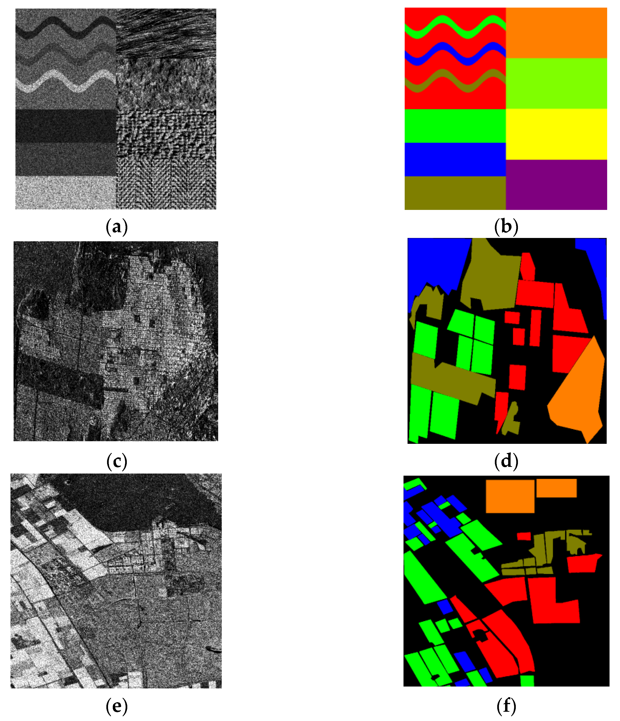
The synthetic image and the groundtruth is given in Figure 4a,b. There are eight categories in the synthetic image. The simulated image consists of three kinds of regions: the narrow curving regions, the homogeneous regions and the textured regions. The narrow curving regions are utilized to assess the detail-preserving capability of the algorithms. The homogeneous regions, especially the textured regions, are utilized to estimate the effect of smoothing. The size of this synthetic image is 486 × 486.

To assess the performance of the GCA-CNN on real scenes, two widely used Radarsat-2 SAR images are used. These two images are obtained on the San Francisco Bay area [16] in America and Flevoland area [16] in the Netherlands. The formatting of the two SAR datasets is single-look-complex, which means that the speckle noise contained in these two images is single-look. The covariance matrices of these two SAR datasets are obtained and the HH components are used to perform the experiments. For the SanFrancisco-Bay data, a widely used sub-image (1010 × 1160 pixels) is selected for the experiments. There are five kinds of terrain in this sub-image. This sub-image and the ground-truth are illustrated in Figure 4c,d. For the Flevoland data, a sub-image with the size of 1000 × 1400 pixels is selected for experiments. 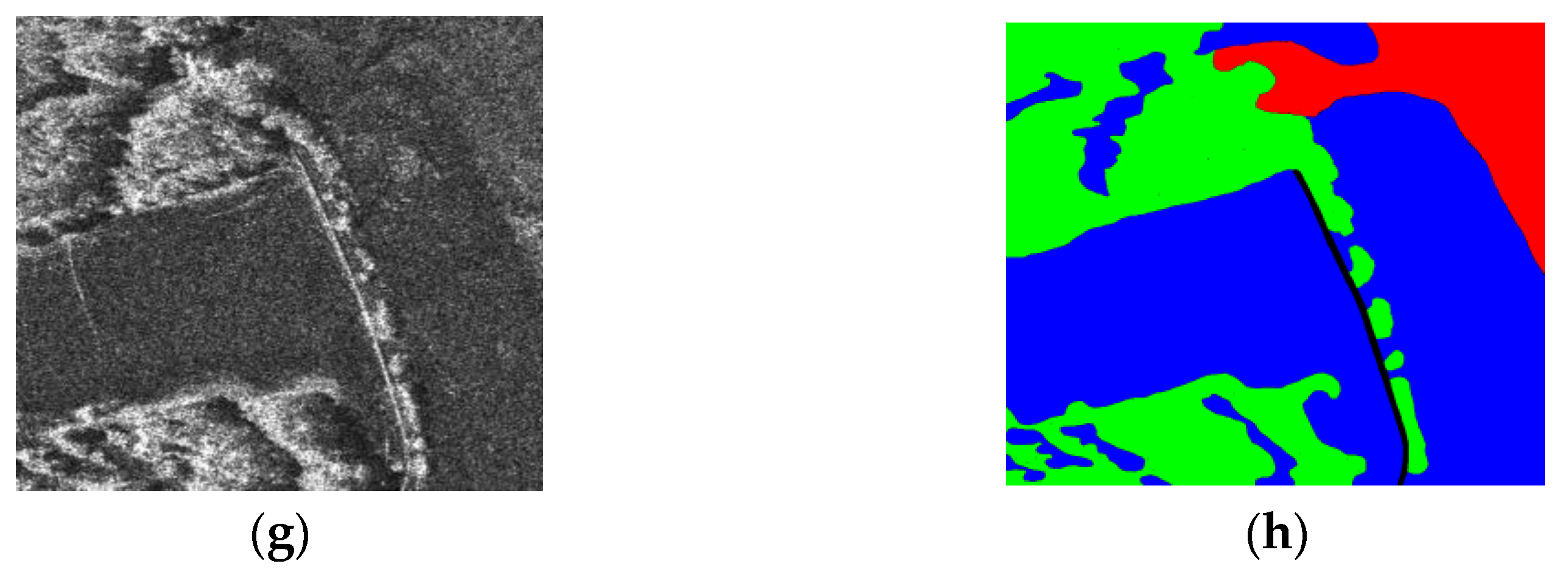The sub-images of the Flevoland with the groundtruth are given in Figure 4e,f, respectively. A TerraSAR-X high-resolution (0.6 m) sub-image obtained from the Lillestroem area is also used for evaluation. This image contains single-look speckle noise and inter-class similarity. Only the HH component is contained in this image. The sub-image and the corresponding groundtruth are given in Figure 4g,h. The size of this sub-image is 1200 × 1600 pixels.

In the utilized images, all the labeled pixels with a fixed size of neighborhood image patch are explored as the samples. The widely used hold-out method is applied to obtain the training and the testing sets, which means that a part of the samples are randomly selected as the training samples while the other samples are used as the testing samples. In our experiments, in order to verify the performance of the proposed algorithm with a limited amount of training samples, the training set only contains 1000 samples [28]. To avoid the overlapping of the training and the testing samples, for each dataset 1000 training samples are randomly selected from the labeled samples, while the remaining labeled samples are utilized as the testing samples.

Some parameters of the GCA-CNN network should be determined before experiments. The size of input image patches should be determined first. In the study, the size of the image patches is set to be 27 × 27 pixels according to the previous work [28]. This size of image patches is determined by experiments in the previous work. The input image patches with too large a size will lead to high time cost and coarse classification results. However, if the size is too small the classification accuracy will be limited due to the lack of spatial neighborhood information.

The structural parameters of the feature-extraction module [29] and the GCA module should then be determined. Structural parameters of the feature-extraction module should be firstly discussed. The feature-extraction module is integrated with a softmax classifier for experiments. To determine how many feature-maps should be included in the convolution layer, the grid researching method is utilized for optimization. According to the work of Zhao et al. 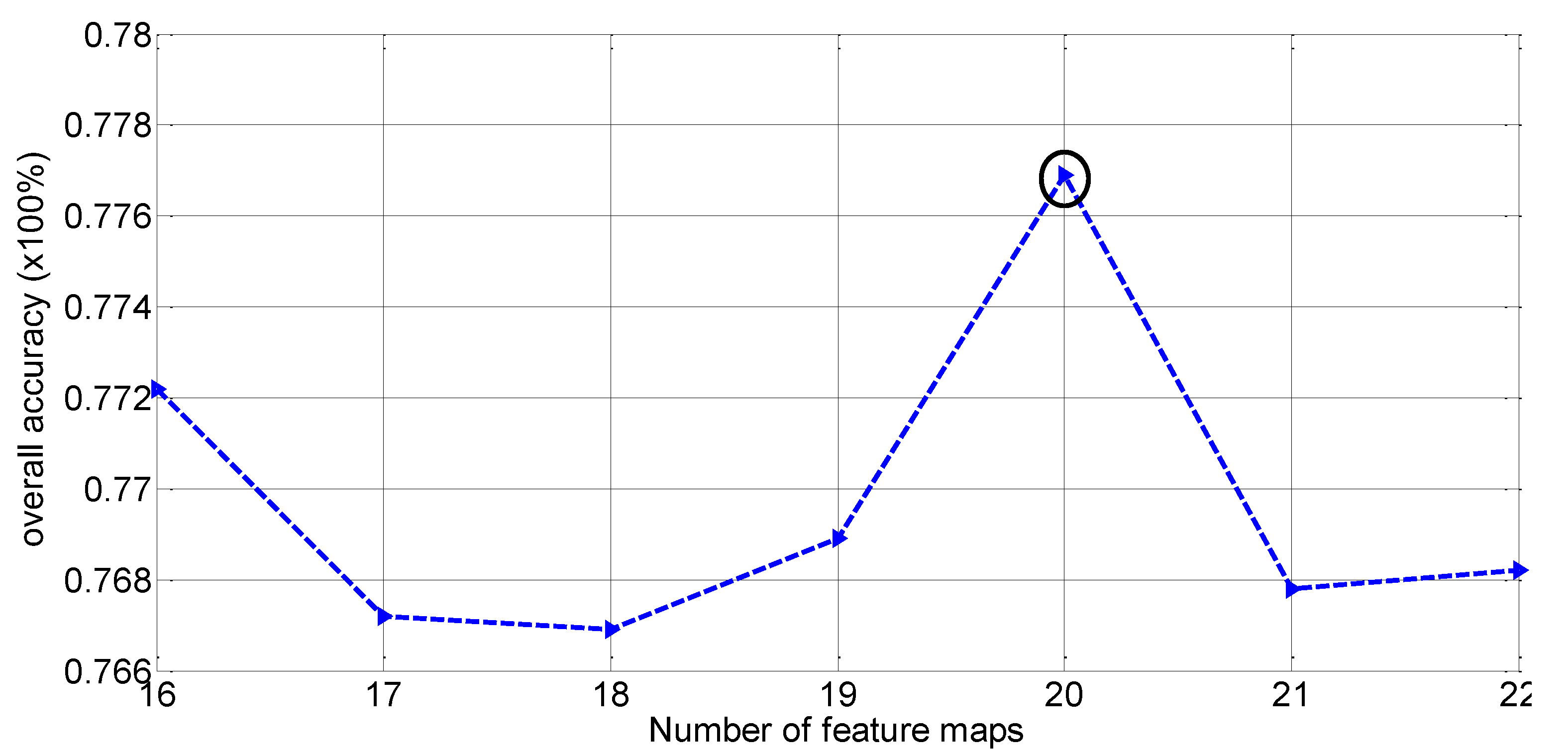[29], each layer owns the same number of feature-maps. The SanFrancisco-Bay SAR image is utilized as the dataset for an example. The results of this optimization are given in Figure 5, where the optimized value of the number of feature-maps is 20, which indicates a tradeoff between the representing capacity and the redundancy of features. In Figure 5 the peaks should be caused by the tradeoff between the representing ability and the redundancy of features. With increasing the number of feature-maps from 16 to 18, the redundancy of the features increases. However, the increase in representing ability cannot offset the affect of the redundancy at this time, which leads to the decrease in overall accuracy. When the number of feature-maps increases from 18 to 20, the increasing representing ability is the dominating factor, which leads to the increase in OA. As the number of feature-maps enlarges further, the redundancy plays a more important role, and the OA decreases again. This causes a peak of OA existing at point of 20.

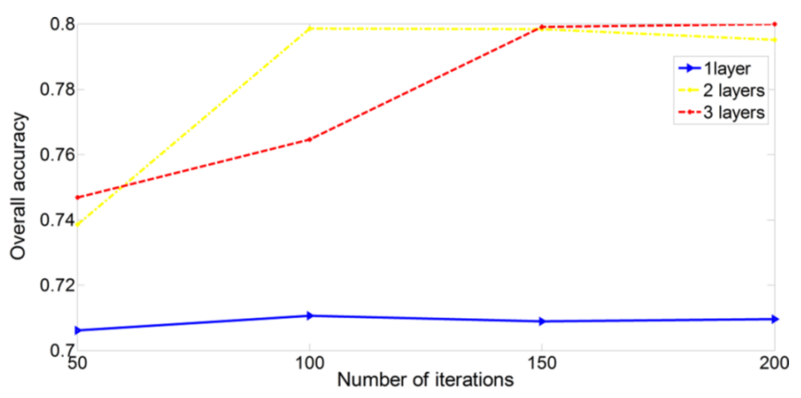
The rest other two parameters, which are the Number Of Iteration (NOI) and the Number Of Layers (NOL), are then optimized. The corresponding results are given in Figure 6, where the optimized NOL and NOI are selected as 2 and 100 (with overall accuracy of 79.33%). Although the CNN module with 3 layers after 150 iterations can achieve a slightly higher accuracy (80.01%), the time cost is much higher. Note that the same optimizations have also been done on the other two datasets and the same optimized value can be obtained. The kernel size in the first convolution layer is set to be 4 and the kernel size in the second convolution layer is set to be 5. The subsampling scale in the pooling layers is set to be 2.

The structural parameters of the GCA module and the classification module are then optimized. For the GCA module, the number of the fully connected layers is the only structural parameter to be optimized. As the amount of training samples is limited, the number of fully connected layers in the GCA module is set to be 2. The size of the kernels in the first convolution layer is 4 and in the second convolution layer is 5.

In order to evaluate the performance of the proposed algorithm, some conventional algorithms such as the Support Vector Machine (SVM) with radial basis function, Deep Belief Network (DBN) and the Stacked Auto-Encoder (SAE) are explored. To verify the effect of the feature fusing, the CNN with the smoothed image (SI-CNN) and the original image (OI-CNN) as the input are also explored. To verify the reasonableness of using the relevance of channels in the feature fusion, the Gated Heterogeneous Fusion Module (GHFM) proposed by Li et al. [15] is explored as the relative state-of-the-art algorithm for comparison.

To quantitatively describe the performance of the proposed and compared algorithms, some popular evaluation metrics are explored in this paper. The Overall Accuracy (OA) can be utilized to evaluate the overall classification accuracy of the algorithms. The OA is calculated as follows:

$$OA=\frac{N_{correct}}{N_{\mathit{total}}}$$

(16)

where N_total means the total number of samples contained in the whole testing set, and the N_correct refers to the number of testing samples which are correctly classified. The classification accuracy in each category is then utilized to evaluate the performance of algorithms in each terrain.

4.2. Results on Synthetic Image

This experiment is performed on the synthetic SAR image. The synthetic SAR image is selected because the boundaries between each two categories are known, which can be used for the evaluation of boundary-locating capability of the proposed and compared algorithms. The detail-keeping capability of the tested algorithms can also be evaluated by using the three narrow curving regions in the upper left part of the synthetic image. The right part of the synthetic image is textured regions with single-look speckle noise which can be utilized to verify the effect of super-pixel based smoothing. In this image there are 486 × 486 labeled samples.

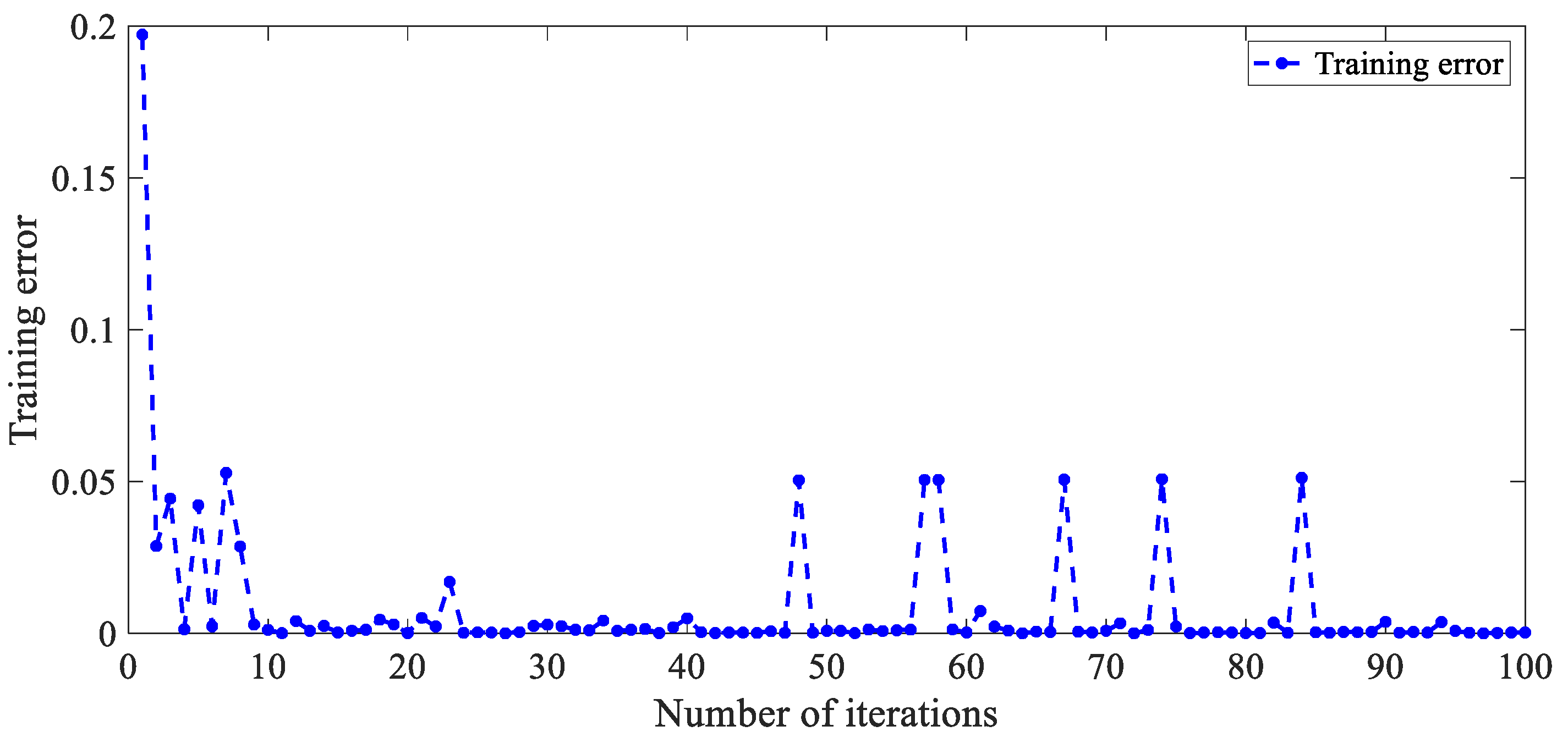
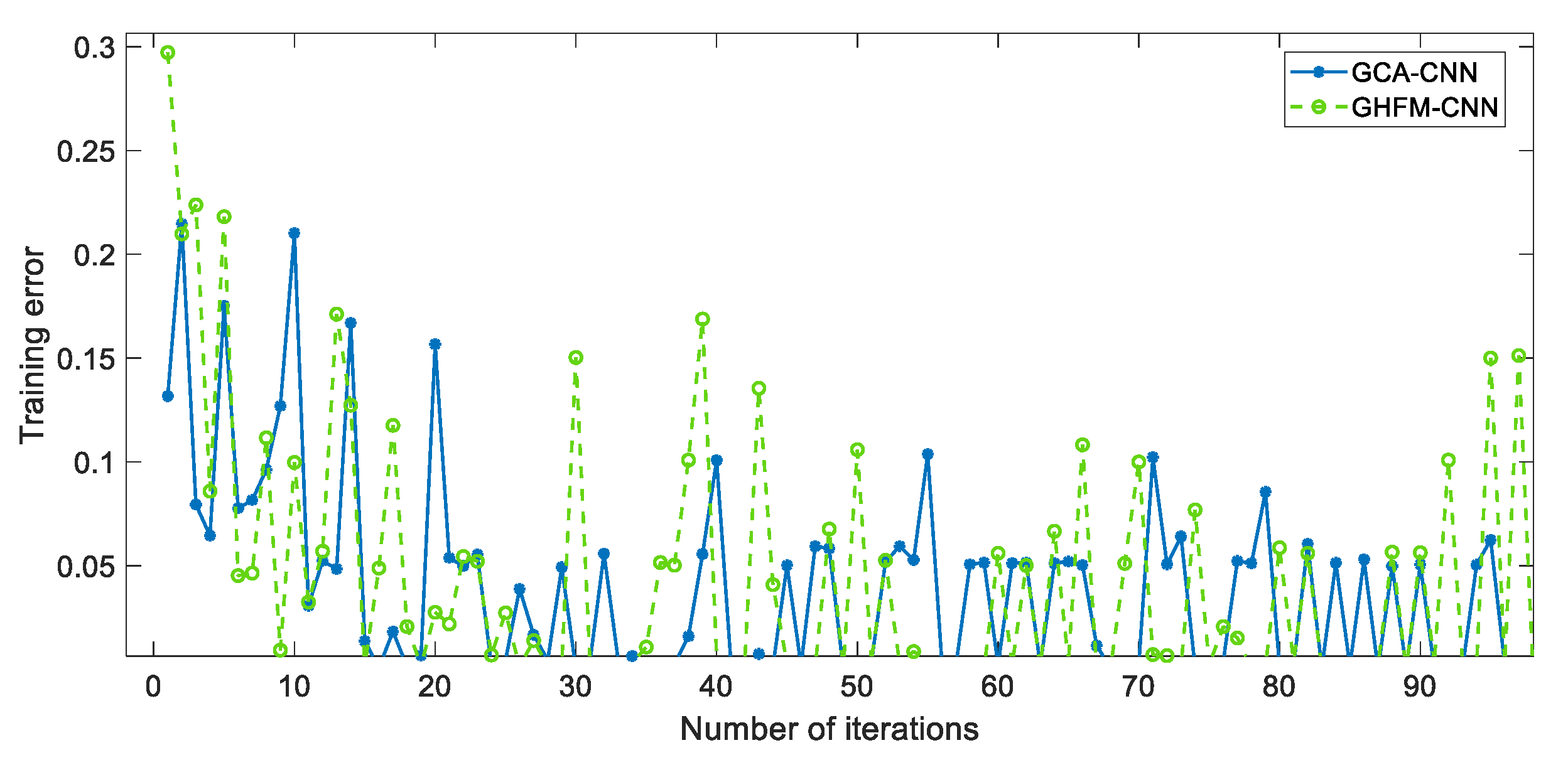
The learning rate of the dual-branches feature-extracted module is experimentally set to be 0.05. The learning rate of the GCA module and the classification module is set to be 0.01. For the DBN, SAE and SVM, the image patches are stretched into feature-vectors to feed into these classifiers. For the SVM, the gamma parameter of kernel is experimentally set to be 0.02 using grid research. The DBN exploited in this paper includes two hidden layers, and both own 100 neurons. The SAE used for comparison has three hidden layers. Each of the first two hidden layers has 200 neurons, while the third layer has 100 neurons. The size of the DBN and SAE are experimentally determined. To verify the reasonableness of the proposed gated channel attention mechanism. The convergence curve of the training error is plotted and demonstrated in Figure 7. As illustrated in Figure 7, the training error gradually converges to 0 (The peak values existed during the iteration number between 40 and 85 might be caused by the outlier samples). This result indicates that for an input sample, an optimized value of gated channel attention coefficients which represents the contribution of feature-maps and the relevance between channels can be obtained. The conclusion above demonstrates the existence of a suitable value of gated channel attention coefficients for an input sample, which proves the reasonableness of the gated channel attention mechanism. In Figure 7, there are some peaks existing in the curve when the training error gradually converges to 0. This can be explained by the training mechanism and the effect of the outliner training samples which are caused by the disturbance of speckle noise. In the explored SGD method 10 samples are randomly selected to form a mini-batch to train the neural network. If the outliner samples are divided into a mini-batch, the updating of the parameters in the GCA-CNN might be wrong, which leads to a small number of peaks in the Figure 7.

The classification accuracies corresponding to the proposed and the compared algorithms are illustrated in

Table 1. Classification results on synthetic SAR image.

Categories	GCA-CNN (%)	GHFM-CNN (%)	SI-CNN (%)	OI-CNN (%)	DBN (%)	SAE (%)	SVM (%)
class 1	95.17	94.77	94.89	95.81	92.98	94.43	86.07
class 2	97.12	97.06	97.94	97.59	97.43	96.26	91.39
class 3	96.22	96.08	96.15	98.10	96.17	96.64	84.14
class 4	98.37	98.65	98.74	98.65	96.43	96.13	96.54
class 5	98.46	97.17	98.01	90.31	96.82	95.51	79.57
class 6	88.38	91.41	91.93	91.73	70.86	73.30	65.44
class 7	93.77	91.25	93.54	90.89	84.21	77.78	82.08
class 8	96.22	96.73	96.36	96.08	94.91	93.60	89.07
OA	95.88	95.13	94.97	94.53	90.74	90.41	85.43

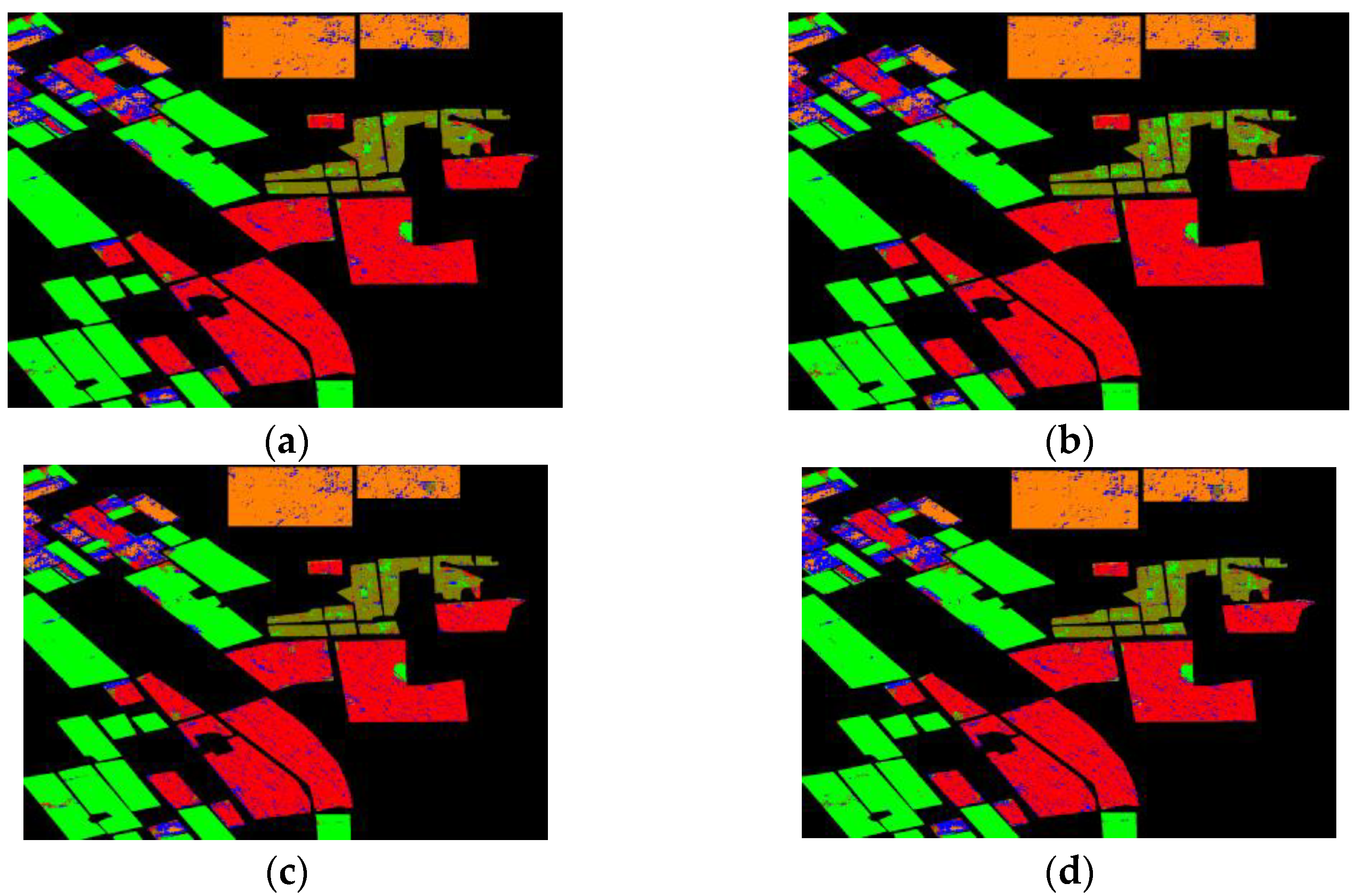
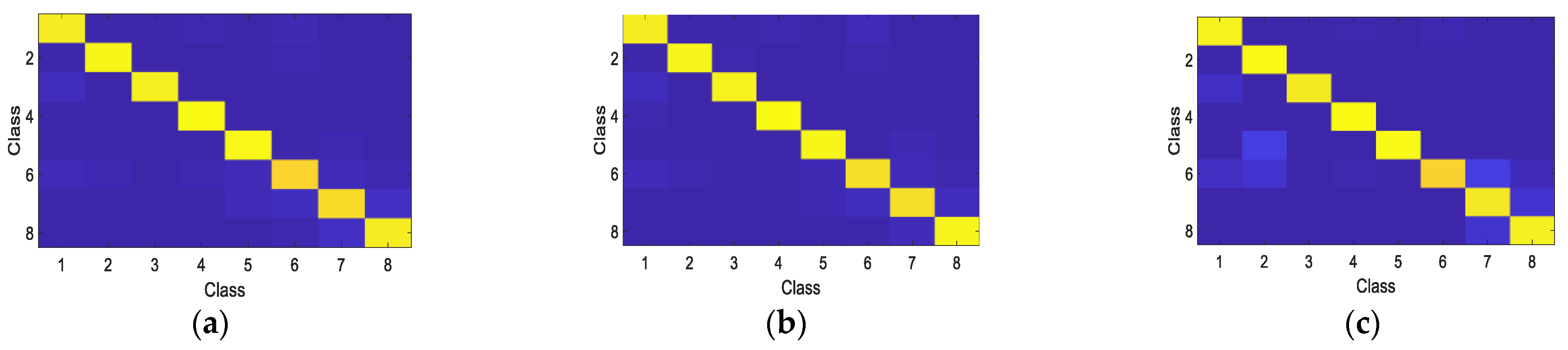
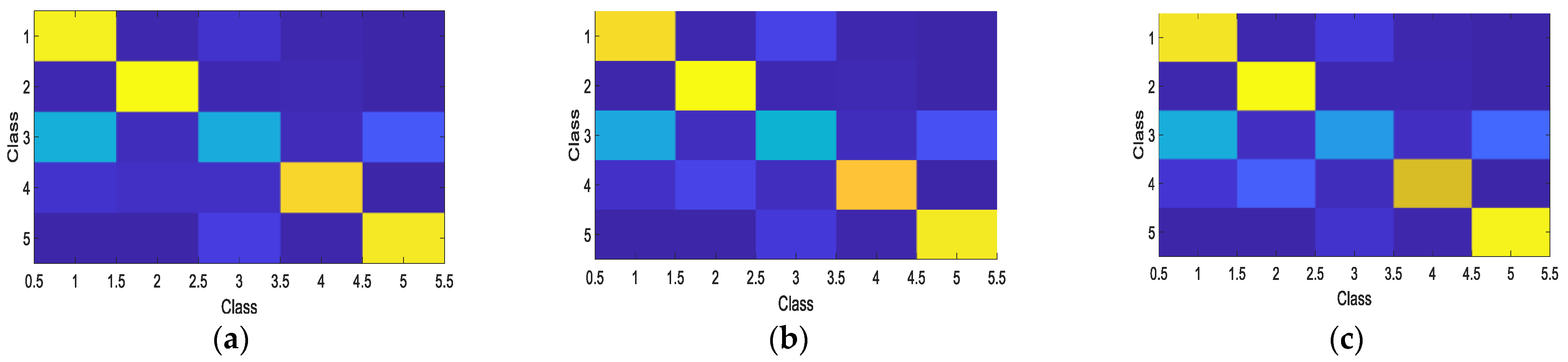
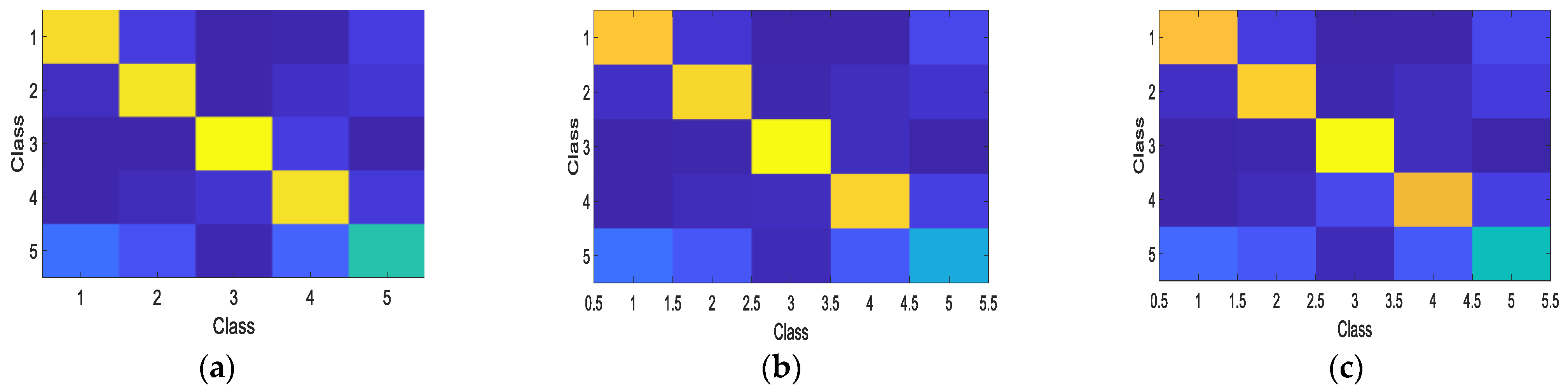
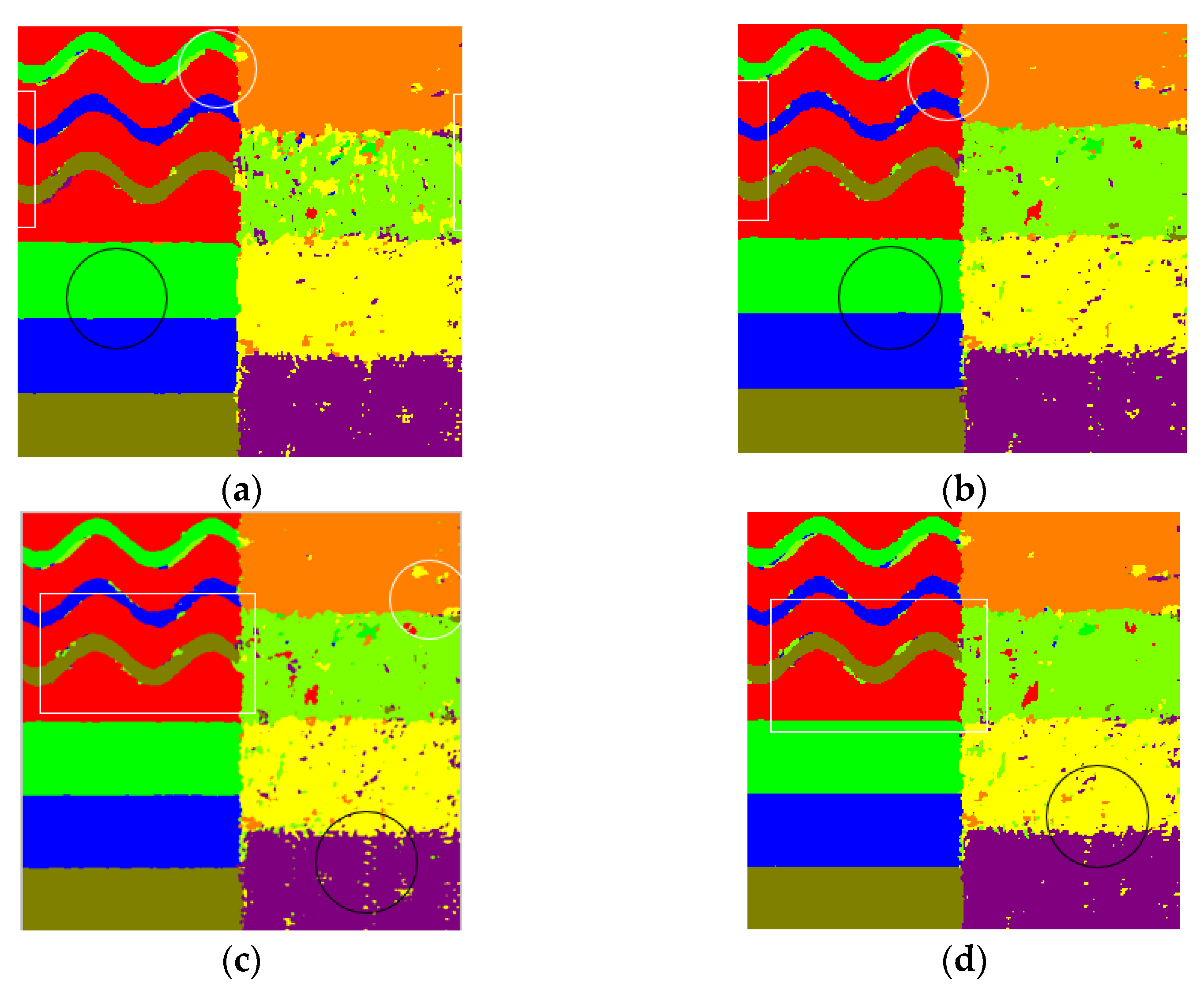
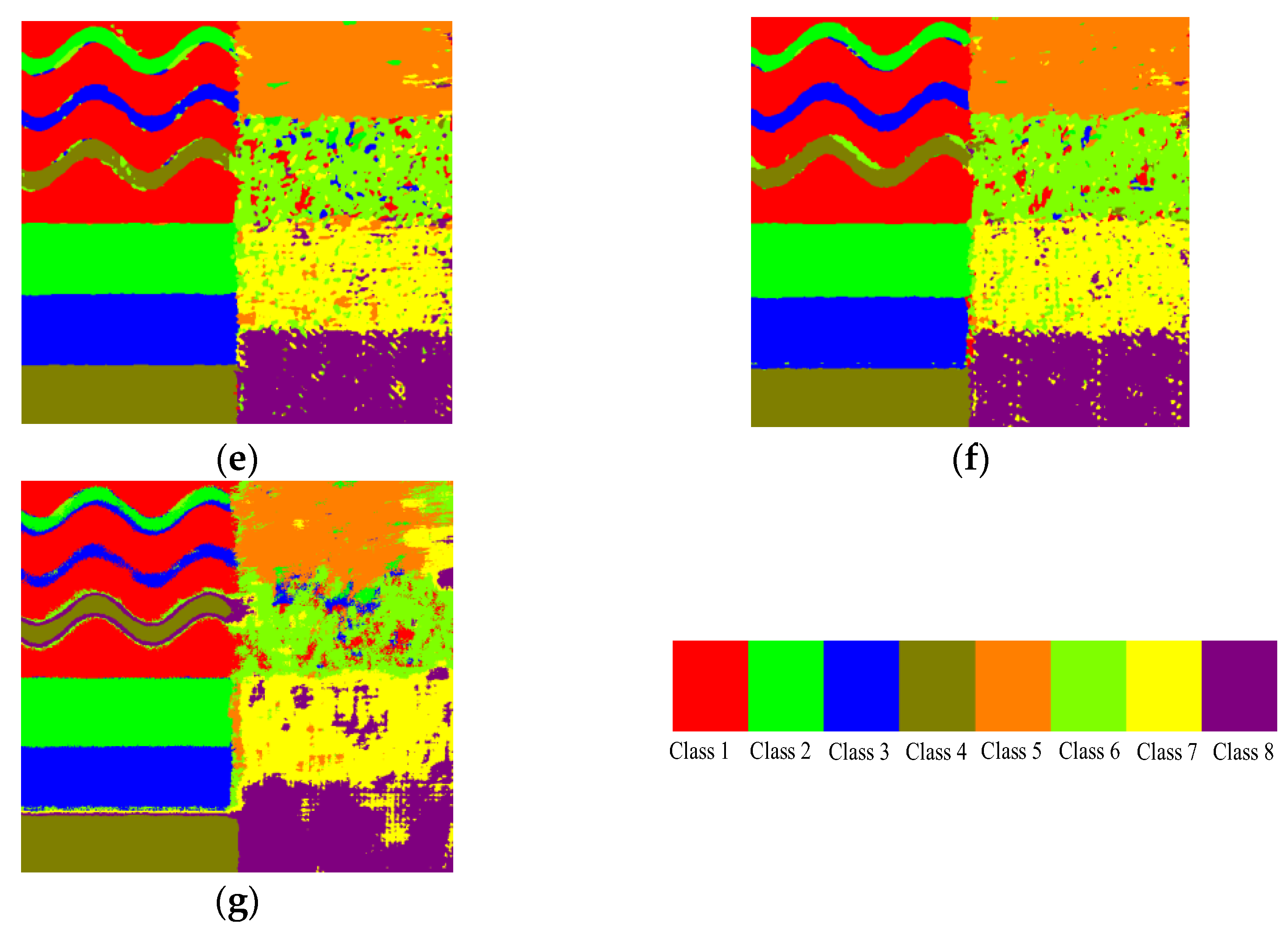
. The results shown in Table 1. The corresponding results in image form are given in Figure 8. The classification accuracies are also illustrated in Figure 9 in the form of confusion matrices for better visualization. As shown in Table 1, the proposed algorithm achieves the highest OA, which demonstrates the superiority of the performance of the GCA-CNN framework.

As shown by the results in Figure 8a, the proposed algorithm shows a combination between the smoothing of misclassification and the detail preserving. Comparing Figure 8b,c, it can be observed that some misclassification in the textured regions is eliminated by the super-pixel based smooth which takes advantage of the spatial neighborhood information (highlighted by circles). However, the detail preserving is weakened by the smoothing, as highlighted by the rectangles in white lines. By fusing the feature-maps, the smoothing of misclassification and the detail preserving can be complementary with each other to produce a better classification result. For the GHFM-CNN, the effect of fusing can be observed on the classification results. By comparing with Figure 8b,c, the fusing of smoothing of misclassification (highlighted by circles) and the detail keeping (highlighted by rectangles) can be seen on Figure 8d. However, by comparing Figure 8d with Figure 8a it can be observed that the smoothing of misclassification and the detail keeping of the GHFM-CNN are less effective than those of GCA-CNN. This result indicates that the proposed GCA fusion module is more effective than GHFM because of utilizing the relevance between channels. The DBN, SAE and SVM show much lower classification accuracy than the CNN because these classifiers are sensitive to speckle noise. The GHFM-CNN algorithm achieves the secondly highest overall accuracy, which indicates that utilizing the relevance between channels is effective for improving the classification accuracy.

In the results maps of these classifiers, there are a large number of misclassified points caused by the disturbance of speckle noise. The DBN, SAE and SVM receive the feature-vectors as input; however, the spatial correlation will be destroyed by stretching the image patches into feature-vectors which leads to the decline of immunity to noise.

However, the proposed GCA-CNN cannot outperform the compared algorithms for all categories. This can be explained by the mechanism of feature fusion. In some conditions, the feature maps extracted from the original image and the smoothed image cannot be complementary with each other. Consequently, the feature fusion will bring feature redundancy, which will lead to a reduction in classification accuracy. Because of this, the GCA-CNN cannot outperform the OI-CNN and the SI-CNN for some categories (such as class 2 and class 4). From another aspect, the training strategy in this paper tends to find the highest overall accuracy for all the explored algorithms. Consequently, the proposed GCA-CNN can outperform the other algorithms on OA but cannot achieve superiority on some categories.

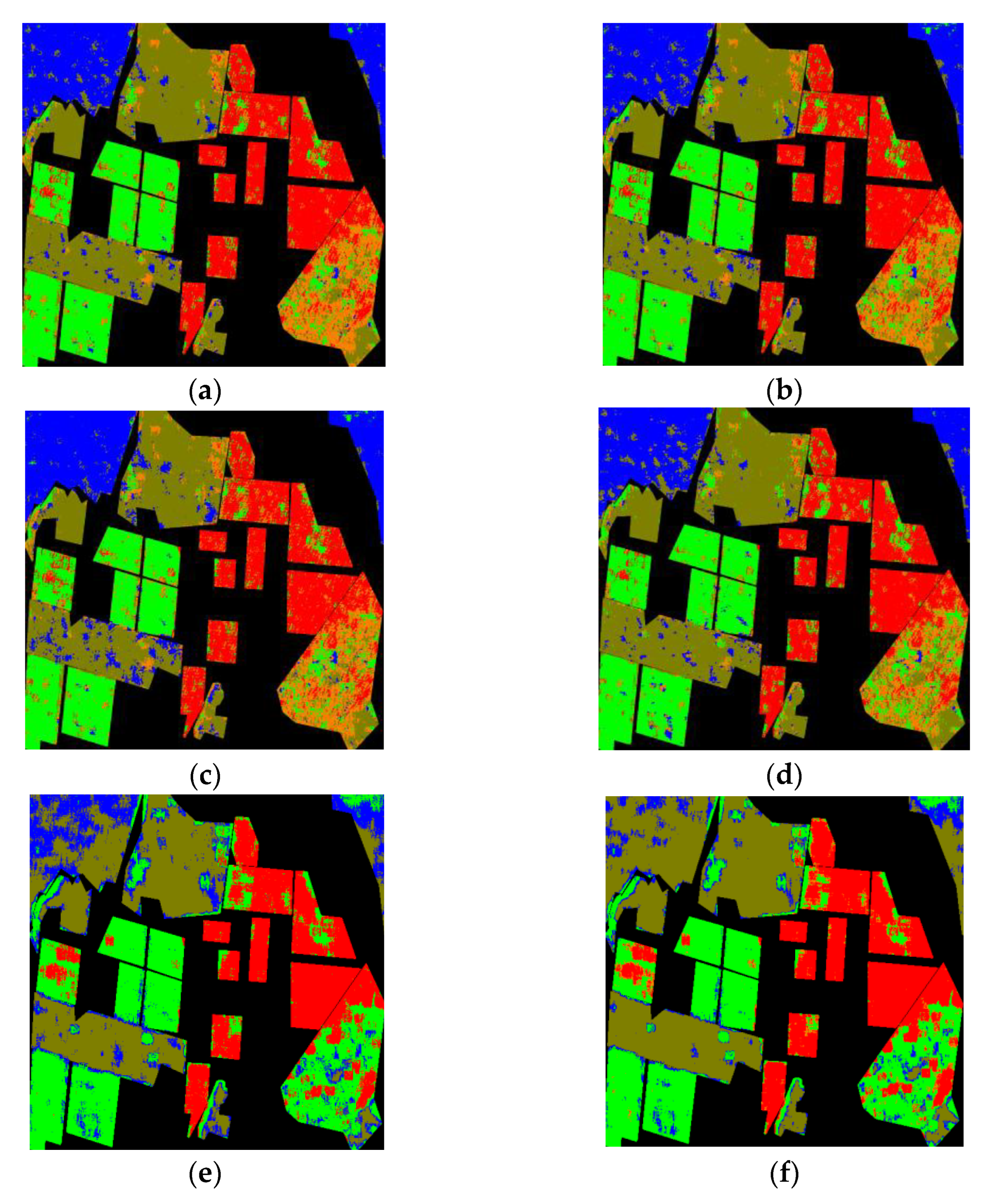
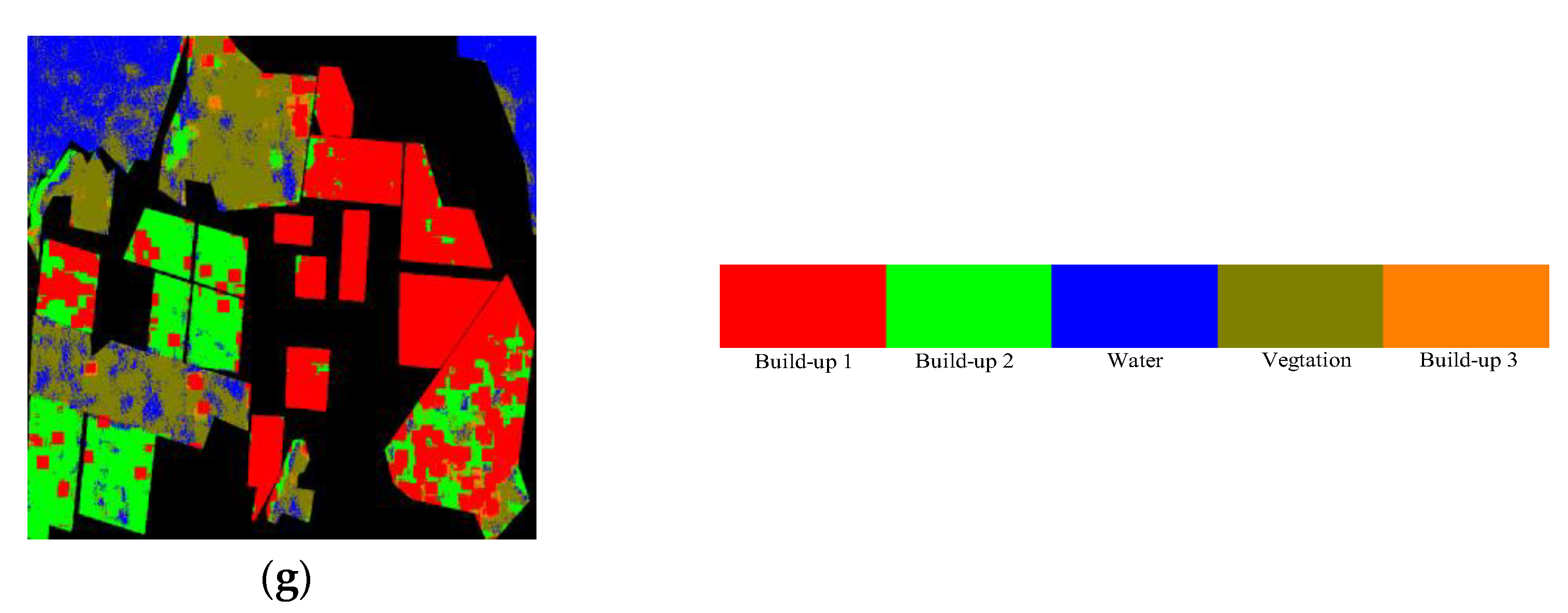
4.3. Results on SanFrancisco-Bay SAR Image

To further prove the superiority of GCA-CNN, the SanFrancisco-Bay SAR image with a high level of noise is explored. For the terrains contained in this image, the homogeneous regions and the boundary regions are included. The homogeneous and boundary regions are mixed to evaluate the fusion effect of smoothing the misclassification and detail keeping. In the explored SAR image there are totally 717,099 samples labeled, and 1000 samples are used as the training samples.

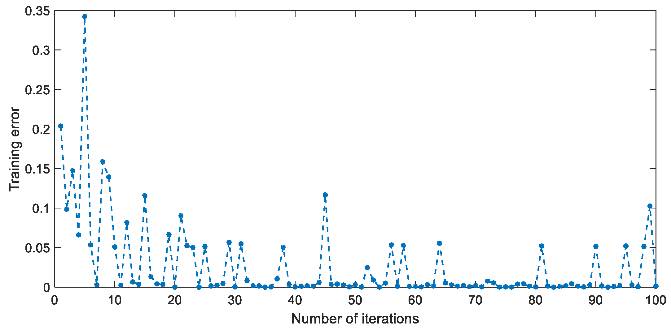
The learning rate of the feature-extraction network of GCA-CNN is also set to be 0.05, while that of the classification network is also experimentally set to be 0.01, which demonstrates the robustness of the parameters of the GCA-CNN framework. The learning rates of CNN are also set to be 0.05. To prove the reasonableness of the proposed gated channel attention coefficients on the real SAR image, the converging curve of the training error as the function of the number of iterations is shown in Figure 10. As given in Figure 10, that training error gradually converges to nearly zero on the real SAR image with high-level noise. This result indicates that the suitable gated channel attention coefficients can be found for a couple of input image-patches, which proves the reasonableness of the proposed gated channel attention mechanism.

For Figure 10, there is a series of alternations of peaks and valleys in the training error curve of the GCA-CNN. This can be explained by the high level of speckle noise and the inter-class similarity on the training samples. Because of these disturbances, the parameters of the GCA cannot converge to the optimized value but wander around the optimized parameters. This mechanism leads to the massive peaks in Figure 10. The OAs and the accuracies for each category of the proposed and compared algorithms are listed in

Table 2. Accuracies of algorithms on SanFrancisco-Bay SAR image.

Categories	GCA-CNN (%)	GHFM-CNN (%)	CNN (%) Smoothed	CNN (%) Original	DBN (%)	SAE (%)	SVM (%)
built-up 1	85.83	83.18	84.92	80.67	89.63	90.65	97.38
built-up 2	86.19	87.29	85.94	84.67	71.36	71.26	75.15
water	91.35	87.86	90.43	95.43	75.88	76.33	77.64
vegetation	85.21	85.74	84.34	77.73	70.84	71.35	70.43
built-up 3	48.49	38.28	43.71	45.27	5.12	4.97	5.78
OA	81.38	79.56	80.63	79.33	64.61	64.97	73.1

for comparison. For better visualization, the corresponding confusion matrices of the GCA-CNN, GHFM-CNN and the OI-CNN are given in Figure 11. In Figure 12, the result maps of all the algorithms are illustrated. In Table 2, it can be observed that the proposed GCA-CNN still achieves the highest OA (81.38%), which demonstrates the superiority of the proposed algorithm over the compared algorithms on the real SAR image. The CNN algorithm with smoothed, and the original SAR image as the input obtains the second and third highest OAs. This result indicates that the superiority of the proposed GCA-CNN derives from the adaptive fusion of FM₁ and FM₂. However, the GHFM-CNN achieves even lower accuracy than the CNN.

This is because the GHFM-CNN contains more parameters than the GCA-CNN, which can lead to over-fitting with limited training samples. As the real SAR image contains high-level noise and more complex features of terrains than the synthetic SAR image, the limited training samples are not enough to optimize the GHFM-CNN. This conclusion can be demonstrated by the converging curve shown in Figure 12. The superiority of GCA-CNN is supported by the classification result map of it (shown in Figure 11a), which shows a combination between smoothing of speckle noise and detail keeping. Comparing Figure 12a with Figure 12b, it can be seen that some isolated misclassified pixels or regions (especially for built-up 3) are eliminated in Figure 12a. This result proves that the smoothing within the super-pixel is effective. Comparing Figure 12a with Figure 12c, there is a conclusion that the superiority of the proposed algorithm derives from the detail keeping. As highlighted by the rectangles in white curves that more details are kept by the GCA-CNN. The classifcation results and the analysis above proved the reasonability of the fusion between FM₁ and FM₂.

For the algorithms which take the feature vector as the input (SAE, DBN and SVM), the corresponding OAs are much lower than those of CNN because these algorithms are vulnerable to noise. The expanding of the 2D image patch into 1D feature vector destroys the spatial correlations between the pixels, which results in lower immunity to noise. As shown in the classification result maps of these algorithms, a lot of misclassified pixels exist which demonstrates the interference of speckle noise.

It should be noted that the DBN, SAE and SVM achieve much higher accuracy on the terrain of build-up 1 than the GCA-CNN. This can be explained by the fact that these three classifiers are not capable enough to discriminate the build-up 1 and the similar terrains. It can be seen from the classification results that the build-up 1 is similar to the build-up 2 and the build-up 3. In addition, these three classifiers show a tendency to classify these terrains into build-up 1. As a result, the DBN, SAE and the SVM show much higher accuracy on build-up 1 than the GCA-CNN.

4.4. Results on Flevoland SAR Image

The Flevoland image is utilized to assess the robustness of GCA-CNN when the level of noise is lower. The terrains contained in the Radarsat-2 Flevoland SAR are less complex than those of SanFrancisco-Bay image, which leads to higher classification accuracy with limited training samples. This experiment explores the Flevoland SAR image to test whether the GCA-CNN can improve the classification accuracy on the SAR image which is easier to be classified. The Flevoland image contains five kinds of terrains. This image contains 539,507 labeled samples, and 1000 samples are selected in a random way to form the training set while the other labeled samples form the testing set.

The learning rate of the feature-extraction network is also experimentally set to be 0.05 while that of the classification network is still set to be 0.01. This result indicates that the parameters of the GCA-CNN framework are robust in different scenes. The learning rate of the CNN is experimentally optimized as 0.05. Structural parameters of the SAE and DBN are kept unchanged. The learning rates of SAE and DBN are experimentally set to be 0.03 and 0.05. To prove the robustness of the proposed GCA fusion module, the converging curve of the training error GCA-CNN on the Flevoland SAR image is illustrated in Figure 13. It can be seen in Figure 13 that the training error gradually converges to zero, which demonstrates the robustness and the reasonableness of the proposed GCA mechanism.

The OAs and the accuracies of all categories of terrains of the proposed and the compared algorithms are given in

Table 3. Accuracies on Flevoland SAR image.

Categories	GCA-CNN (%)	GHFM-CNN (%)	CNN (%) Original	CNN (%) Smoothed	DBN (%)	SAE (%)	SVM (%)
forest	88.83	87.21	87.92	90.79	96.59	86.64	87.38
farmland 1	96.83	95.73	95.94	96.47	96.18	82.33	96.87
farmland 2	34.79	33.75	33.43	33.69	29.35	10.26	32.64
urban	76.63	75.12	75.34	74.46	43.61	68.53	54.73
water	94.77	94.38	94.41	94.26	73.46	99.02	97.33
OA	86.62	85.27	85.48	85.63	81.30	81.51	82.71

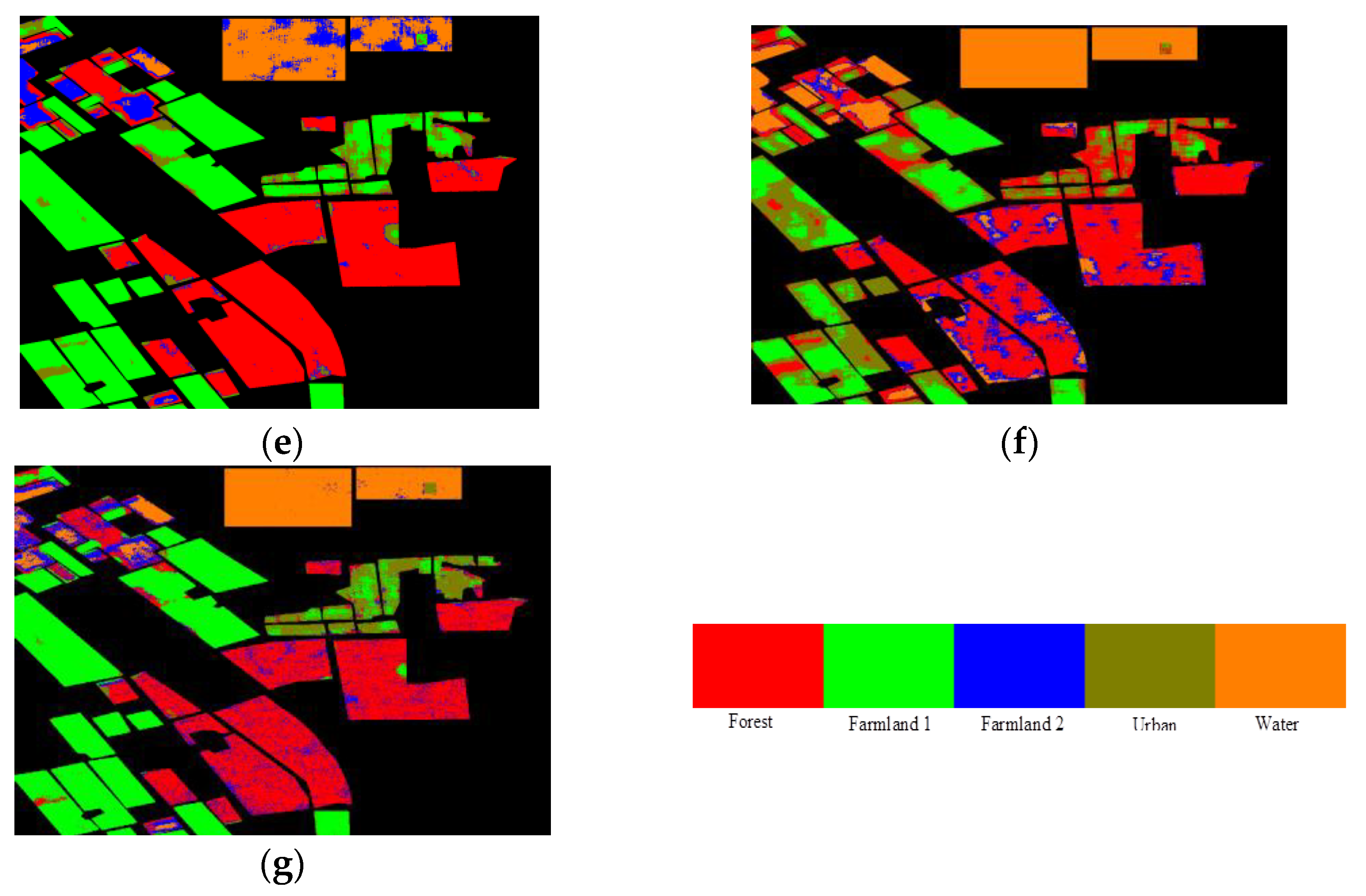
. The accuracies shown in Table 3 are illustrated in Figure 14 in the form of confusion matrices for more intuitive visualization. The results of these algorithms are given in Figure 15 for analysis. The GCA-CNN still achieves the highest OA. However, the improvement in OA brought by GCA-CNN is less obvious because the Flevoland SAR image is easier to be classified. The OAs obtained by the CNN with the original and smoothed SAR image as input are the second and third highest. Different from the other experiments, the CNN with the original image as the input image achieves higher OA than that with smoothed image as the input. This is because the interclass similarity caused by the speckle noise is lower than that of the synthetic SAR image and the SanFrancisco-Bay SAR image. The conclusion can be supported by the fact that the misclassified regions caused by the speckle noise existing in Flevoland image are much fewer than those in the SanFrancisco image.

As a result, in this real SAR image the detail keeping is more important than the smoothing of speckle because the noise level in this image is relatively lower. However, the super-pixel based smoothing may damage the details in the SAR image. Consequently, the CNN algorithm with the original image as the input obtains the higher OA.

The classification accuracy of GHFM-CNN is still lower than that of CNN because of the overfitting. The result demonstrates the superiority of the GCA module over the GHFM module. Firstly, the proposed GCA module explored the relevance between the channels of feature-maps, which is not considered by the GHFM. Secondly, the structure of GCA is simpler than that of GHFM, which leads to less parameters. As a result, the parameters of the GCA module can be trained with limited training samples. The DBN, SAE, SVM achieve lower overall accuracy than CNN and because of that these frameworks are vulnerable to speckle noise.

4.5. Results on TerraSAR-X SAR Image

The TerraSAR-X image with a high resolution of 0.6m is explored to evaluate the performance of the proposed GCA-CNN. This image contains three kinds of terrain, which are the forest, grass and the river. This image is used to evaluate the performance of the GCA-CNN on the high-resolution SAR image. The learning rates of the GCA module and the other parts of the GCA-CNN are set to be 0.01 and 0.05. For fair comparison, 1000 labeled samples are randomly selected for the training of GCA-CNN while the other labeled samples are left for the testing. The learning rate of the CNN is experimentally optimized as 0.05.

The experimental results of the GCA-CNN and the compared algorithms are given in

Table 4. Accuracies onTerraSAR-X SAR image.

Categories	OI-CNN (%)	SI-CNN (%)	GCA-CNN (%)	GHFM-CNN (%)
River	21.21	18.01	25.76	25.69
Forest	81.08	83.31	83.96	83.01
Grass	89.18	92.48	92.51	91.33
OA	79.62	81.76	82.44	82.24

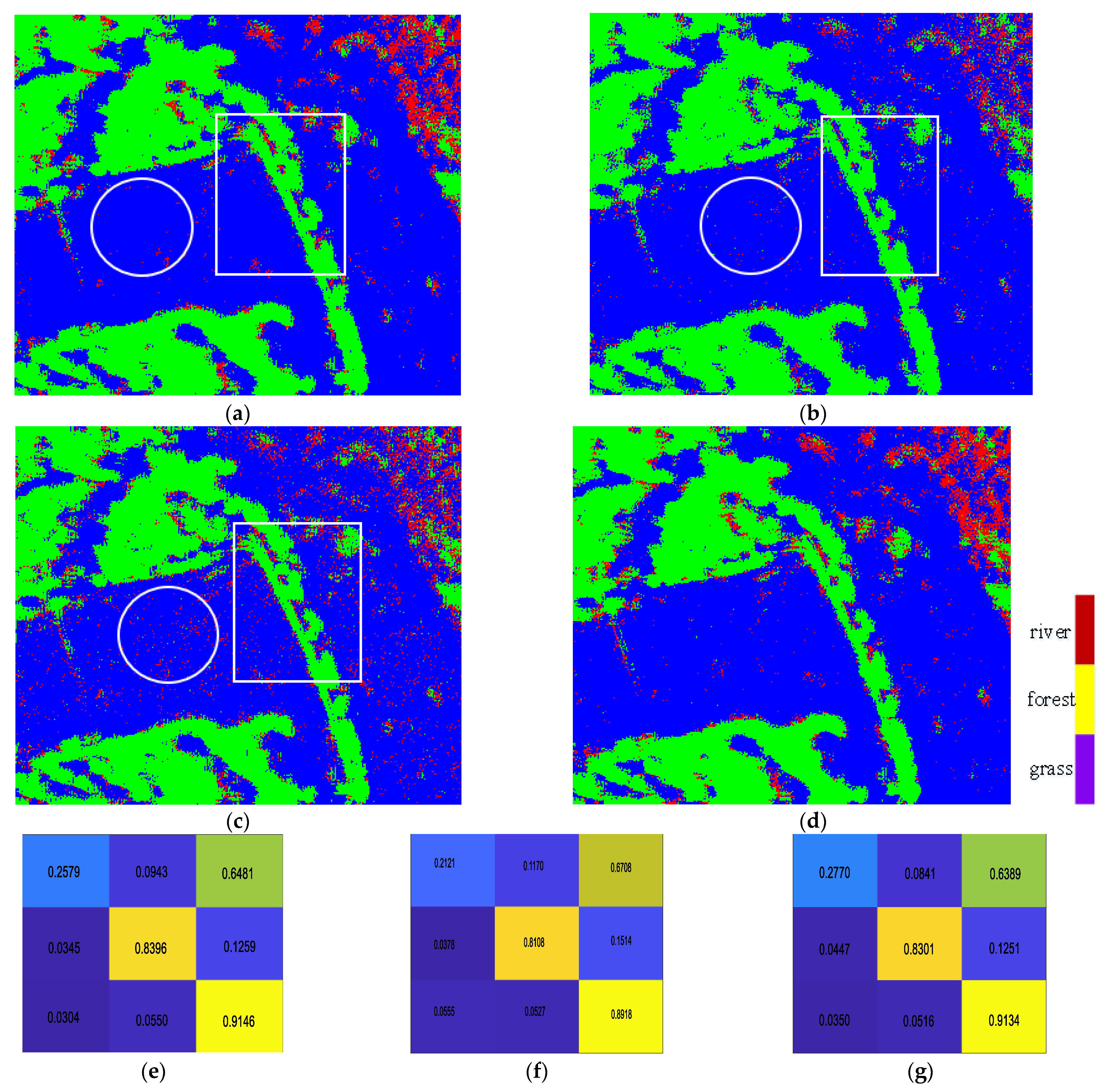
. The DBN, SAE and the SVM are vulnerable to speckle noise, which leads to low classification accuracies. The classification results of these algorithms are not listed for discussion. The corresponding confusion matrices are shown in Figure 16a for better visualization. For the sake of comparison, the accuracies are listed on the confusion matrices. The accuracies of the explored algorithms are then discussed according to result-maps. The mechanism of the combination of gated and channel attention is also discussed. From Table 4, it can be seen that the GCA-CNN can still achieve the highest classification accuracy among the explored algorithms in the high resolution image. As this image contains massive speckle noise and terrains with high inter-class similarity (such as the river), the proposed algorithm brings more than 3% improvement in the overall accuracy. This result demonstrates that the proposed GCA-CNN is effective for the classification of high-resolution SAR images with massive speckle noise. The GHFM-CNN based algorithms still reach the second highest overall accuracy, which demonstrates the superiority of the GCA-based fusion strategy. The super-pixel based smoothing also brings nearly 2% improvement in overall accuracy, which is caused by the high-level speckle noise in the TerraSAR-X image.

The classification results maps is shown in Figure 16 for discussions and demonstration. By comparing Figure 16a with Figure 16b,c, it indicates that the GCA-CNN can adaptively fuse the features of the original image and the smoothed image and complement them. Comparing Figure 16b,c, it can be seen that the results of the SI-CNN are much smoother than those of OI-CNN. However, the boundaries are much clearer and details (especially the ones highlighted by the white rectangle) are better preserved in Figure 16c. For the GCA-CNN, the advantages of both OI-CNN and the SI-CNN are absorbed. From the aspect of the reduction in speckle noise, by comparing Figure 16a with Figure 16c it can be seen that Figure 16a is much smoother than Figure 16c (highlighted by the white circle). For the details keeping, the boundaries in Figure 16a are clearer and the details (highlighted by the white rectangle) are better preserved than Figure 16b. By investigating the classificstion results of the terrain river, which is easy to misclassify due to its inter-class similarity, it can be seen that the results in Figure 16a make a complementary with those of Figure 16b,c. The discussion made above can be supported by the Figure 16e,f. The accuracy of river is obviously enhanced (about 4%) by the adaptive fusion. This conclusion indicates that the GCA fusion module can adaptively emphasize the features of the original image and the smoothed image for classifying the terrains with higher accuracy.

The mechanism of the GCA fusion module will be explained in a way of visualization. As the GCA is constructed by integrating the gated mechanism and the channel attention mechanism, the mechanism of GCA will be illustrated from two aspects: the emphasis of the contribution of feature-maps, and the difference in contribution between channels. An image patch containing the boundaries is cropped from the SAR image as the data resource for validation.

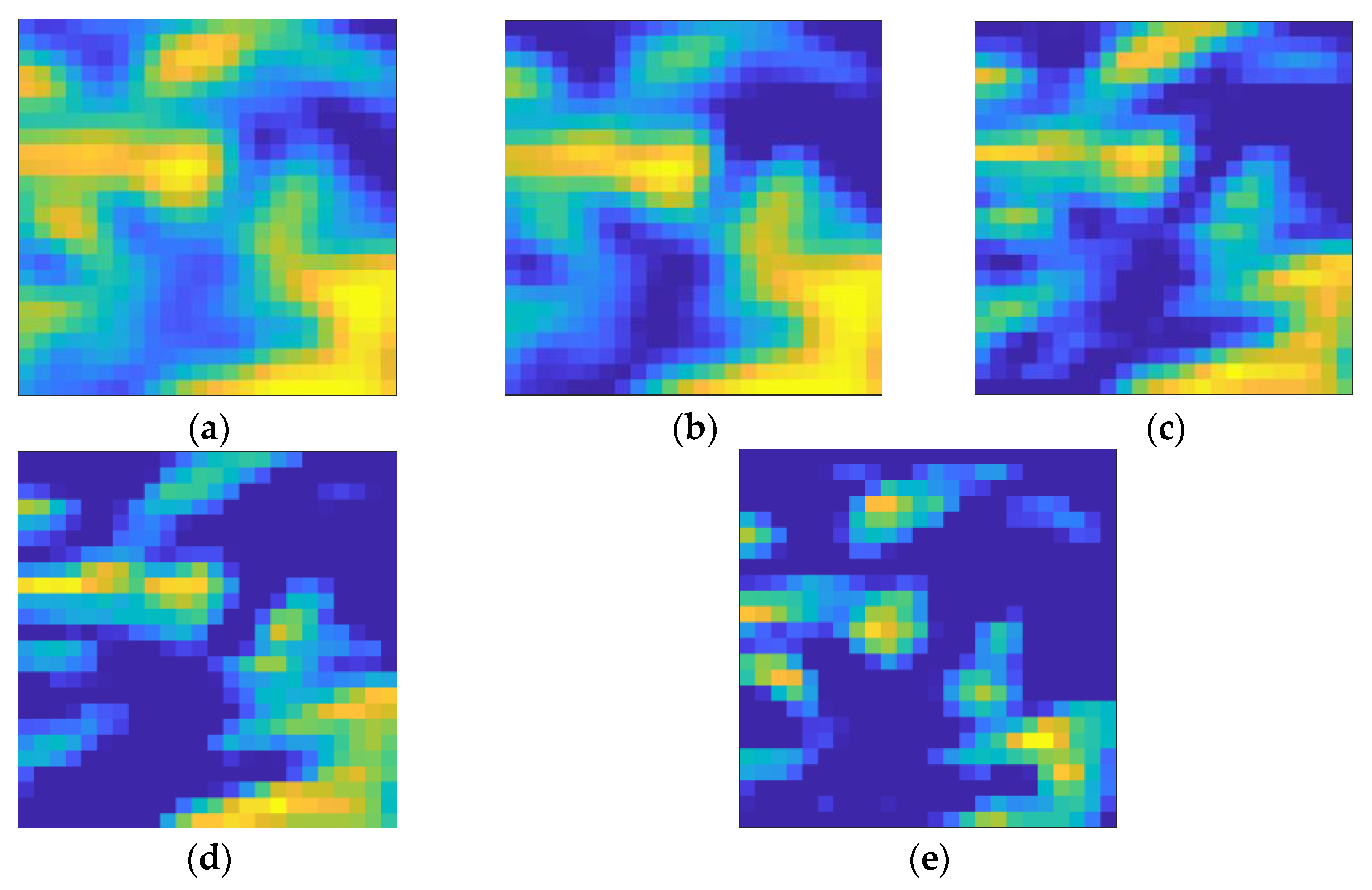
For the first aspect, two image patches from the original image and the smoothed image are shown in Figure 17a,b. Two feature maps extracted separately from the original image and the smoothed image are explored for comparison. These two feature maps are illustrated in Figure 17c,d, where it can be seen that the feature map from the original image contains more information of boundaries, while the feature map from the smoothed image contains less information on the boundaries. As calculated by the GCA module, the fusion coefficients of these two feature maps are 0.6937 and 0.3063, which gives the feature map extracted from the original image higher weight.

For the second aspect, two feature maps extracted from the original image are used for validation and these are shown in Figure 17c,e. There are clear differences between these two feature maps because the corresponding convolution kernels are different. Consequently, the contribution of these feature maps on classification are different. As calculated by GCA, the fusion coefficients of these two feature maps are 0.6937 and 0.2582, which shows an obvious difference. This result demonstrates that the difference between channels is well considered by the GCA module.

4.6. Discussions on the Effectiveness of the Adaptive Fusion

The superiority of the proposed GCA modules derives from two aspects: (1) the combination of Gated mechanism and channel attention mechanism; and (2) the strategy of adaptive fusion. To demonstrate the effectiveness of the adaptive fusion, some discussion will be made in this section. As shown in Figure 8b,c, the results show a complementarity between the OI-CNN and the SI-CNN. The CNN taking the super-pixel based smoothed image as the input can eliminate some misclassifications in the texture regions. On the other hand, the CNN which takes the original image as the input shows better boundary-keeping ability. As discussed above, for different kind of regions, the features corresponding to the smoothed image and the original image should have different impacts. For the texture regions, the original image is more important, and the smoothed image will be more important for the smoothed image. To quantitatively assess the effectiveness of the adaptive fusion, a fusion strategy with Equal Weights is explored for comparison. The corresponding classification network is denoted as EW-CNN. The comparison of results between the GCA-CNN, EW-CNN and the OI-CNN is shown in Figure 18.

In Figure 18, it can be seen that the performance of the EW-CNN is obviously lower than the GCA-CNN. For the real SAR images with complex characters of terrains, the performance of EW-CNN is even lower than the OI-CNN. This phenomenon is caused by the inappropriate fusion which reduces the discrimination of the features, and consequently leads to lower classification accuracy. By the discussion above, the effectiveness of the adaptive fusion can be proved.

4.7. Discussions on the Computational Complexity

The computational complexity of the proposed GCA-CNN and the compared algorithms is also discussed in this paper. The time complexity and the spatial complexity of these algorithms are discussed separately. For the conventional CNN, the time complexity can be expressed as: O(${\displaystyle {\sum }_{l=1}^D{M}_l^2{K}_l^2{C}_{l-1}{C}_l}+{\displaystyle {\sum }_{n=1}^N{F}_{n-1}{F}_n}$). In this expression, D and N denote the number of convolution layers and fully connected layers, respectively. The number K_l refers to the size of convolution kernels in the l^th layer, M_l refers to the size of the feature-maps in the l^th layer, C_l means the number of feature-maps in the l^th convolution layer, while F_n refers to the number of neurons in the n^th fully connected layer. Thus, for the explored CNN in this paper, the time complexity can be calculated as: O(27² × 4² × 20 + 12² × 5² × 20² + 320 × k), where k is the number of categories. For the GCA-CNN, the time complexity is calculated as O(2 × 27² × 4² × 20 + 2 × 12² × 5² × 20² + 320 × k + 20 × 40) (two branches, a fully connected layer in the GCA fusion module and a fully connected layer in the classifier module). It can be seen that the time complexity of the GCA-CNN is about twice that of CNN. However, the time cost of the GCA-CNN can be reduced by a half through the parallel computation of the two branches of GCA-CNN on two GPUs. As discussed above, the proposed GCA-CNN shows a tradeoff between the classification accuracy and the time cost. The DBN and the SAE are composed of fully connected layers, thus the time complexities of these two models are calculated as: O(27² × 100 + 100² + 100 × k) and O(27² × 200 + 200² + 200 × 100 + 100 × k), respectively. It can be seen that the time complexity of the GCA-CNN is larger than DBN and SAE, however, the GCA-CNN can achieve much higher classification accuracy. For the SVM the time complexity is calculated as O(27²N_s), where N_s is the number of support vectors. It can be seen that the SVM achieves the lowest time complexity.

For the spatial complexity, the DBN and SAE own obviously larger spatial complexity than the GCA-CNN and CNN because of the following two reasons: firstly, the numbers of neurons in DBN and SAE are much larger than those of GCA-CNN and CNN; and secondly, the mechanisms of local connection and weights sharing in the GCA-CNN and CNN reduce the spatial complexity significantly. The SVM still obtains the lowest spatial complexity, because only the support vectors make a contribution on the optimization of the parameters of SVM.

5. Conclusions

In this paper, a novel GCA-CNN network is proposed for the SAR image classification. This network consists of the dual-branches feature-extraction module, the proposed GCA feature fusion module and the classification module. The feature-extraction module receives the original image and super-pixel based smoothed image as the input. In the GCA module, a novel gated channel attention mechanism is proposed for the adaptive fusion of feature-maps by embedding the relevance between channels into the conventional gated mechanism. By the adaptive feature fusion, enhancing the overall accuracy and detail keeping can be realized at the same time. The effectiveness of the proposed GCA is demonstrated by experiments. The experimental results demonstrate the effectiveness of the proposed framework and the superiority over the compared algorithms. In the future, a new fusion strategy which considers the interaction between dual branches among multi-layers should be proposed based on the GCA. Furthermore, the relevance between channels should be considered by using the second order statistical property of the SAR image.

References

1. Krizhevsky, A.; Sutskever, I.; Hinton, G. ImageNet classification with deep convolutional neural networks. Adv. Neural Inf. Process. Syst. 2012, 25, 1097–1105. [Google Scholar] [CrossRef] [Green Version]
2. He, K.; Zhang, X.; Ren, S.; Sun, J. Deep Residual Learning for Image Recognition. In Proceedings of the IEEE Conference on Computer Vision and Pattern Recognition, Las Vegas, NV, USA, 27–30 June 2016; pp. 770–778. [Google Scholar]
3. Szegedy, C.; Liu, W.; Jia, Y.; Sermanet, P.; Reed, S.; Anguelov, D.; Rabinovich, A. Going deeper with convolutions. In Proceedings of the IEEE Conference on Computer Vision and Pattern Recognition, Boston, MA, USA, 7–12 June 2015; pp. 1–9. [Google Scholar]
4. Simonyan, K.; Zisserman, A. Very deep convolutional networks for large-scale image recognition. In Proceedings of the International Conference on Learning Representations, San Diego, CA, USA, 7–9 May 2015; pp. 1–14. [Google Scholar]
5. Zhou, Y.; Wang, H.; Xu, F.; Jin, Y. Polarimetric SAR Image Classification Using Deep Convolutional Neural Networks. IEEE Geosci. Remote Sens. Lett. 2016, 13, 1935–1939. [Google Scholar] [CrossRef]
6. Zhang, Z.; Wang, H.; Xu, F.; Jin, Y.Q. Complex-valued convolutional neural network and its application in polarimetric SAR image classification. IEEE Trans. Geosci. Remote Sens. 2017, 55, 7177–7188. [Google Scholar] [CrossRef]
7. Tan, X.; Li, M.; Zhang, P.; Wu, Y.; Song, W. Complex-valued 3-D convolutional neural network for PolSAR image classification. IEEE Geosci. Remote Sens. Lett. 2019, 17, 1022–1026. [Google Scholar] [CrossRef]
8. Duan, Y.; Liu, F.; Jiao, L.; Zhao, P.; Zhang, L. SAR image segmentation based on convolutional-wavelet neural network and markov random field. Pattern Recognit. 2017, 64, 255–267. [Google Scholar] [CrossRef]
9. Hou, B.; Kou, H.; Jiao, L. Classification of polarimetric SAR images using multilayer autoencoders and superpixels. IEEE J. Sel. Top. Appl. Earth Obs. Remote Sens. 2016, 9, 3072–3081. [Google Scholar] [CrossRef]
10. Liu, H.; Yang, S.; Gou, S.; Zhu, D.; Wang, R.; Jiao, L. Polarimetric SAR feature extraction with neighborhood preservation-based deep learning. IEEE J. Sel. Top. Appl. Earth Obs. Remote Sens. 2017, 10, 1456–1466. [Google Scholar] [CrossRef]
11. Chen, Y.; Jiang, H.; Li, C.; Jia, X.; Ghamisi, P. Deep feature extraction and classification of hyperspectral images based on convolutional neural networks. IEEE Trans. Geosci. Remote Sens. 2016, 54, 6232–6251. [Google Scholar] [CrossRef] [Green Version]
12. Zhang, A.; Yang, X.; Fang, S.; Ai, J. Region level SAR image classification using deep features and spatial constraints. ISPRS J. Photogramm. Remote Sens. 2020, 163, 36–48. [Google Scholar] [CrossRef]
13. Gao, F.; Huang, T.; Wang, J.; Sun, J.; Amir, H.; Yang, E. Dual-branch deep convolution neural network for polarimetric SAR image classification. Appl. Sci. 2017, 7, 447. [Google Scholar] [CrossRef]
14. Liang, W.; Wu, Y.; Li, M.; Cao, Y.; Hu, X. High-resolution SAR image classification using multi-scale deep feature fusion and covariance pooling manifold network. Remote Sens. 2021, 13, 328. [Google Scholar] [CrossRef]
15. Li, X.; Lei, L.; Sun, Y.; Li, M.; Kuang, G. Collaborative attention-based heterogeneous gated fusion network for land cover classification. IEEE Trans. Geosci. Remote Sens. 2020, 59, 3829–3845. [Google Scholar] [CrossRef]
16. Zhang, L.; Ma, W.; Zhang, D. Stacked sparse autoencoder in PolSAR data classification using local spatial information. IEEE Geosci. Remote Sens. Lett. 2016, 13, 1359–1363. [Google Scholar] [CrossRef]
17. Liu, F.; Jiao, L.; Hou, B.; Yang, S. PolSAR image classification based on Wishart DBN and local spatial information. IEEE Trans. Geosci. Remote Sens. 2016, 54, 3292–3308. [Google Scholar] [CrossRef]
18. Jie, H.; Li, S.; Gang, S.; Albanie, S. Squeeze-and-excitation networks. IEEE Trans. Pattern Anal. Mach. Intell. 2017, 42, 2011–2023. [Google Scholar]
19. Lécun, Y.; Bottou, L.; Bengio, Y.; Haffner, P. Gradient-based learning applied to document recognition. Proc. IEEE 1998, 86, 2278–2324. [Google Scholar] [CrossRef] [Green Version]
20. He, K.; Zhang, X.; Ren, S.; Sun, J. Delving Deep into Rectifiers: Surpassing Human-Level Performance on ImageNet Classification. Available online: https://arxiv.org/abs/1502.01852 (accessed on 2 February 2015).
21. Wang, Q.; Liu, S.; Chanussot, J.; Li, X. Scene classification with recurrent attention of VHR remote sensing images. IEEE Trans. Geosci. Remote Sens. 2018, 57, 1155–1167. [Google Scholar] [CrossRef]
22. Tong, W.; Chen, W.; Han, W.; Li, X.; Wang, L. Channel-attention-based DenseNet network for remote sensing image scene classification. IEEE J. Sel. Top. Appl. Earth Obs. Remote Sens. 2020, 13, 4121–4132. [Google Scholar] [CrossRef]
23. Zhao, Z.; Li, J.; Luo, Z.; Li, J.; Chen, C. Remote sensing image scene classification based on an enhanced attention module. IEEE Geosci. Remote Sens. Lett. 2020, 18, 1926–1930. [Google Scholar] [CrossRef]
24. Mei, X.; Pan, E.; Ma, Y.; Dai, X.; Huang, J.; Fan, F.; Ma, J. Spectral-spatial attention networks for hyperspectral image classification. Remote Sens. 2019, 11, 963. [Google Scholar] [CrossRef] [Green Version]
25. Yu, C.; Han, R.; Song, M.; Liu, C.; Chang, C.I. Feedback Attention-Based Dense CNN for Hyperspectral Image Classification. IEEE Trans. Geosci. Remote Sens. 2021, 60, 1–16. [Google Scholar] [CrossRef]
26. Ma, F.; Gao, F.; Sun, J.; Zhou, H.; Hussain, A. Attention graph convolution network for image segmentation in big SAR imagery data. Remote Sens. 2019, 11, 2586. [Google Scholar]
27. Achanta, R.; Shaji, A.; Smith, K.; Lucchi, A.; Fua, P.; Süsstrunk, S. SLIC superpixels compared to state-of-the-art superpixel methods. IEEE Trans. Pattern Anal. Mach. Intell. 2012, 34, 2274–2282. [Google Scholar] [CrossRef] [Green Version]
28. Zhang, A.; Yang, X.; Jia, L.; Ai, J.; Xia, J. SRAD-CNN for adaptive Synthetic Aperture Radar image classification. Int. J. Remote Sens. 2018, 40, 3461–3485. [Google Scholar]
29. Zhao, W.; Du, S. Spectral–spatial feature extraction for hyperspectral image classification: A dimension reduction and deep learning approach. IEEE Trans. Geosci. Remote Sens. 2016, 54, 4544–4554. [Google Scholar] [CrossRef]
Figure 1. The structure of LeNet-5.
Remotesensing 15 00362 g001
Figure 2. The workflow of the proposed GCA-CNN.
Remotesensing 15 00362 g002
Figure 3. The structure of the proposed GCA-CNN network.
Remotesensing 15 00362 g003
Figure 4. The explored SAR images and the corresponding groundtruth: (a) The synthetic SAR image; (b) Groundtruth of the synthetic SAR image; (c) The SanFrancisco-Bay SAR image (Radarsat-2); (d) The groundtruth of the SanFrancisco-Bay SAR image; (e) The Flevoland SAR image (Radarsat-2); (f) The groundtruth of the Flevoland SAR image; (g) The Lillestroem TerraSAR-X SAR image; (h) The groundtruth of the Lillestroem TerraSAR-X image.
Remotesensing 15 00362 g004aRemotesensing 15 00362 g004b
Figure 5. Optimizing the Number of feature maps.
Remotesensing 15 00362 g005
Figure 6. The optimized results of NOL and the NOI.
Remotesensing 15 00362 g006
Figure 7. The convergence curve of the training error on the synthetic image.
Remotesensing 15 00362 g007
Figure 8. The classification result maps on the synthetic SAR image: (a) The results of the GCA-CNN; (b) The classification results of the SI-CNN; (c) The results of the OI-CNN; (d) The results of GHFM-CNN; (e) The results of the DBN; (f) The results of the SAE; (g) The results of the SVM.
Remotesensing 15 00362 g008aRemotesensing 15 00362 g008b
Figure 9. The confusion matrices of: (a) GCA-CNN; (b) GHFM-CNN; and the (c) OI-CNN on the synthetic SAR image.
Remotesensing 15 00362 g009
Figure 10. The converging curve of GCA-CNN and GHFM-CNN on the SanFrancisco-Bay image.
Remotesensing 15 00362 g010
Figure 11. The confusion matrices of the (a) GCA-CNN, (b) GHFM-CNN and (c) OI-CNN on the SanFransisco-Bay image.
Remotesensing 15 00362 g011
Figure 12. The classification result maps on the SanFrancisco-Bay SAR image: (a) The classification results of the GCA-CNN; (b) The classification results of the SI-CNN; (c) The classification results of the OI-CNN; (d) The classification results of the GHFM-CNN; (e) The classification results of the DBN; (f) The classification results of the SAE; (g) The classification results of the SVM.
Remotesensing 15 00362 g012aRemotesensing 15 00362 g012b
Figure 13. The converging curve of GCA-CNN on the Flevoland image.
Remotesensing 15 00362 g013
Figure 14. The confusion matrices of (a) GCA-CNN, (b) GHFM-CNN and the (c) OI-CNN.
Remotesensing 15 00362 g014
Figure 15. The classification result on the Flevoland SAR image: (a) The results of the GCA-CNN; (b) The results of the SI-CNN; (c) The results of the OI-CNN; (d) The results of the GHFM-CNN; (e) The results of the DBN; (f) The results of the SAE; (g) The results of the SVM.
Remotesensing 15 00362 g015aRemotesensing 15 00362 g015b
Figure 16. The classification results on TerraSAR image: (a) Results of the GCA-CNN; (b) Results of the OI-CNN; (c) Results of the SI-CNN; (d) Results of the GHFM-CNN. (eg) The confusion matrices of the GCA-CNN, OI-CNN and the GHFM-CNN of TerraSAR image (For better visualization).
Remotesensing 15 00362 g016
Figure 17. The visualization of image patches and the corresponding feature-maps: (a) The image patch extracted from the original image; (b) The image patch extracted from the smoothed image; (c) a feature-map of the original image patch; (d) a feature-maps of the smoothed image patch; (e) a different feature-map of the original image patch.
Remotesensing 15 00362 g017
Figure 18. Accuracies of GCA-CNN, OI-CNN and the EW-CNN on three datasets.
Remotesensing 15 00362 g018