Numerical Modeling of Land Surface Temperature over Complex Geologic Terrains: A Remote Sensing Approach

Abstract

A physically-based image processing approach, based on a single-source surface energy balance framework, is developed here to model the land surface temperature (LST) over complex/rugged geologic terrains at medium to high spatial resolution (<10² m). This approach combines atmospheric parameters with a bulk-layer soil model and remote-sensing-based parameterization schemes to simulate surface temperature over bare surfaces. The model’s inputs comprise a digital elevation model, surface temperature data, and a set of land surface parameters including albedo, emissivity, roughness length, thermal conductivity, soil porosity, and soil moisture content, which are adjusted for elevation, solar time, and moisture contents when necessary. High-quality weather data were acquired from a nearby weather station. By solving the energy balance, heat, and water flow equations per pixel and subsequently integrating the surface and subsurface energy fluxes over time, a model-simulated temperature map/dataset is generated. The resulting map can then be contrasted with concurrent remote sensing LST (typically nighttime) data aiming to remove the diurnal effects and constrain the contribution of the subsurface heating component. The model’s performance and sensitivity were assessed across two distinct test sites in China and Iran, using point-scale observational data and regional-scale ASTER imagery, respectively. The model, known as the Surface Kinetic Temperature Simulator (SkinTES), has direct applications in resource exploration and geological studies in arid to semi-arid regions of the world.

1. Introduction

Land surface temperature (LST) is a critical state variable relevant to many land surface processes that is generally derived from thermal infrared remote sensing data [1,2,3]. LST has been used in several applications within the field of geology and natural resources [4,5,6], although it is predominantly used for mapping and monitoring thermal anomalies associated with geothermal and volcanic activities [7,8,9,10,11,12].

In geological studies, temperature measurements are assumed to arise from the combined effects of surface and subsurface processes, with the latter component being of fundamental importance to characterize and differentiate. However, owing to the prevailing effects of diurnal solar heating, the subsurface heating component is confidently recognized only when it presents a pronounced contrast against the background temperature trend [8,11,13]. In the majority of cases, though, the subsurface temperature signal becomes indistinguishable from the background mostly due to heterogeneity in the heating rates of surface and near-surface materials. This complexity is caused by multiple factors, encompassing meteorological forcing, surface physical properties (i.e., surface albedo, emissivity, thermal inertia, and surface roughness length), topography, vegetation cover, and soil moisture availability [5,13,14]. The cumulative effect of these factors has significantly restricted the practical application of remotely sensed LST data in geology and resource exploration.

To avoid the disturbances caused by topography and solar heating, LST has been commonly acquired during nighttime. Nevertheless, residual solar heating effects can persist until the pre-dawn hours [11,12,15,16]. Several methods have been proposed to remove the diurnal effects from remotely sensed LST data. These methods range from using a variable-sized box-shaped moving window to define a background temperature against which anomalous temperatures are characterized (e.g., [9]), to simplified statistical techniques deployed to determine a surface temperature baseline from which the topographic effects are removed [17]. The spatial-based insolation model introduced by Fu and Rich [18] represents another approach used to mitigate the solar and topographic effects in remote sensing temperature data. Coolbaugh, Kratt, Fallacaro, Calvin, and Taranik [7] developed empirical relationships to correct for surface albedo, thermal inertia, and topographic slope effects, aiming to generate a pseudo-temperature image that can be subtracted from the corresponding LST data. This approach has been further refined by Gutiérrez, et al. [19] by accounting for the altitude lapse rate effects. More recently, Malbéteau, et al. [20] developed an energy balance model for normalizing satellite-derived LST, accounting for illumination and elevation effects in topographically rugged terrains, assuming uniform albedo and emissivity values across the entire modeling domain.

Land surface modeling based on energy balance equations attempts to rigorously model energy and water exchanges at the interface of land and atmosphere using a combination of physical and empirical models [21]. Land surface models (LSMs) are widely used for mapping evapotranspiration [22,23,24], estimating soil moisture contents [25], modeling climatological variations and surface temperature patterns [1,26,27,28,29], and correcting the cooling effects of clouds on LST [30,31].

The majority of existing LSMs are developed for and applied to studies conducted at either point scale (10⁰ m) or regional and global scales (>10³ m) [1,25,32,33,34]. Spatial resolutions of >10² m, however, are considered too coarse for detailed mapping and modeling of surface temperature patterns in geologically heterogeneous environments [8]. At this scale, topography comprises a major source of spatial heterogeneity in the distribution of surface solar radiation and atmospheric forcing, the neglect of which can introduce significant uncertainties in modeling results [20,32,35]. In addition, the spatial heterogeneity introduced by complex geologic terrains is often inadequately integrated into the modeling processes. Thus far, investigations into the potential use of LSMs to quantitatively model and correct diurnal heating effects within medium- to high-resolution surface temperature data have been limited. Romaguera, Vaughan, Ettema, Izquierdo-Verdiguier, Hecker, and van der Meer [32] represent perhaps the only study of this kind, that assessed the application of the Noah LSM to correcting coarse-resolution (i.e., 3.5 km) geostationary satellite data at the mesoscale.

In this context, we introduce SKinTES (Surface Kinetic Temperature Simulator), a single-source energy balance model tailored specially for modeling LST dynamics over complex geological areas spanning hundreds to thousands of square kilometers. Developed in the Interactive Data Language (IDL) environment (Version 8.1, NV5 Geospatial Software), the code aims to overcome the limitations encountered when correcting LST data at sub-100 m scales for diurnal and terrain effects, although it can be used as a general tool for surface temperature modeling. The underlying hypothesis of the approach is that by modeling and removing the effects of diurnal temperature variations, one can uncover the subtle temperature anomalies (of either positive or negative form) associated with subsurface geologic processes. SKinTES is explicitly designed to retrieve the LST over bare surfaces and surfaces with sparse vegetation cover (defined by NDVI < 0.2) and is applicable under clear-sky conditions with minimal cloud cover and precipitation. A notable advantage of the model is its independence from in situ measurements, except for weather data, which are typically acquired from nearby weather stations. The model is built upon satellite-based parameterization schemes for parameter estimation and model implementation, with the capability to explicitly account for complex geology and rugged topography.

This article presents the theoretical basis of the model, outlines its parameterization schemes, and provides the first results obtained by applying the model to simulate surface temperature patterns at two distinct sites in China and Iran. The studies are conducted at two different spatial scales (point and regional scale) and across varying elevation ranges. The application of the model to specific geologic studies will be covered in a separate article.

2. Model Description

Assuming that the ground surface is a homogeneous medium, the temperature can be described by the following one-dimensional heat flow equation:

$$\frac{\mathsf{\partial }T}{\mathsf{\partial }t}=\mathsf{\kappa }\frac{{\mathsf{\partial }}^{2}T}{{\mathsf{\partial }z}^2}$$

(1)

where $T$ ($\mathrm{K}$), $t$ (s), and $z$ ($\mathrm{m}$) are temperature, time, and depth, respectively, and $\mathsf{\kappa }$ is thermal diffusivity (${\mathrm{m}}^2\cdot {\mathrm{s}}^{-1}$) with a dependency on soil moisture content. The surface energy balance equation at the earth–atmosphere interface determines the upper boundary condition:

$$S_g+R_a-R_g-H-\mathsf{\lambda }E-G=0$$

(2)

where $S_g$ ($\mathrm{W}\cdot {\mathrm{m}}^{-2}$) is the global shortwave solar radiation, $R_a$ is the downwelling longwave radiation from the atmosphere, $R_g$ is the upwelling longwave radiation from the ground, $H$ is the sensible heat flux, $\mathsf{\lambda }E$ is the latent heat flux, and $G$ is the surface heat flux positive downward. The expression of each term of the energy budget is given below.

2.1. Solar Radiation (Insolation)

The global broadband shortwave solar radiation ($S_g$) over rugged terrain is expressed as:

$$S_g=S_b+S_d+S_r$$

(3a)

where $S_b$, $S_d$, and $S_r$ are direct beam solar irradiance, diffuse irradiance from the sky, and adjacent terrain-reflected irradiance, respectively. The direct solar radiation is modeled as:

$$S_b=\left(1-{\mathsf{\alpha }}_g\right) \frac{G_{sc}}{d^2}\cos {\mathsf{\phi }}_z^{\prime }{\mathsf{\tau }}_b$$

(3b)

where $G_{sc}$ is the solar constant ($=1366.1 \mathrm{W}\cdot {\mathrm{m}}^{-2}$), $1/d^2$ is the relative Earth–Sun distance, ${\mathsf{\tau }}_b$ is the beam transmittance of the atmosphere defined in Appendix A, ${\mathsf{\phi }}_z^{\prime }$ is the local solar illumination angle (the angle between the normal to the surface and the sun), and ${\mathsf{\alpha }}_g$ (-) is the broadband surface albedo defined in Section 3.2.1. By using the slope (${\mathsf{\beta }}_S$) and aspect (${\mathsf{\beta }}_A$) angles derived from a digital elevation model (DEM), the local illumination angle of a sloping surface could be calculated:

$$\cos \hspace{0.17em}{\mathsf{\phi }}_z^{\prime }=sin\left({\mathsf{\phi }}_e\right)cos\left({\mathsf{\beta }}_S\right)+cos\left({\mathsf{\phi }}_e\right)sin\left({\mathsf{\beta }}_S\right)cos({\mathsf{\phi }}_a-{\mathsf{\beta }}_A)$$

(3c)

where ${\mathsf{\phi }}_e$ and ${\mathsf{\phi }}_a$ are the solar elevation angle and the solar azimuth angle, respectively, both of which are assumed to be spatially uniform at each given time.

The diffuse sky irradiance by the atmosphere on a slopping surface is formulated as [36]:

$$S_d=\left(1-{\mathsf{\alpha }}_g\right)\frac{G_{sc} }{d^2}\cos \hspace{0.17em}{\mathsf{\phi }}_z{V}_d {\mathsf{\tau }}_d$$

(3d)

where ${\mathsf{\phi }}_z$ is the solar zenith angle, $V_d$ (-) is the sky view factor (${0<V}_d\le 1$) defined as the ratio of diffuse sky irradiance at a pixel to the total possible irradiance on a flat surface under isotropic diffuse illumination conditions [37], and ${\mathsf{\tau }}_d$ is the diffuse transmittance of the atmosphere that together with ${\mathsf{\tau }}_b$ in Equation (3b) are parametrized by Yang’s model [38,39] (see Appendix A), recognized as one of the most reliable models for retrieving solar irradiance [40].

The terrain-reflected irradiance is expressed by:

$$S_r=\left(1-{\mathsf{\alpha }}_g\right)\overline{I_r} \overline{{\mathsf{\alpha }}_g} C_t$$

(3e)

where $\overline{{\mathsf{\alpha }}_g}$ is the average albedo of the adjacent terrain, and $C_t$ (-) is the terrain configuration factor (${0<C}_t\le 1$) defined as the area of surrounding slopes visible to the target point approximated by Dozier and Frew [36] as:

$$C_t\approx \frac{1+\cos \hspace{0.17em}{\mathsf{\beta }}_S}{2}-V_d$$

(3f)

$\overline{I_r}$ in Equation (3e) is the average irradiance arriving at adjacent slopes at a radius of about 0.5–1 km calculated by using $\cos \hspace{0.17em}\overline{{\mathsf{\phi }}_z^{\prime }}$ and $\overline{V_d}$ to approximate the direct and diffuse sky irradiance, respectively:

$$\overline{I_r}\approx \frac{G_{sc}}{d^2}(\mathit{cos}\hspace{0.17em}\overline{{\mathsf{\phi }}_z^{\prime }}{\mathsf{\tau }}_b+\mathit{cos}\hspace{0.17em}{\mathsf{\phi }}_z\overline{V_d} {\mathsf{\tau }}_d)$$

(3g)

Here, $\cos \hspace{0.17em}\overline{{\mathsf{\phi }}_z^{\prime }}$ is obtained by substituting the average slope ($\overline{{\mathsf{\beta }}_S}$) and aspect ($\overline{{\mathsf{\beta }}_A}$) in Equation (3c), and $\overline{V_d}$ is the average sky view factor of the neighboring pixels.

2.2. Longwave Radiations

The upwelling longwave radiation from the ground is calculated using Equation (4):

$$R_g={\mathsf{\epsilon }}_g\mathsf{\sigma }{T}_g^4$$

(4)

where $\mathsf{\sigma }$ is the Stephan–Boltzmann constant ($=$5.67 $\times$ 10⁻⁸ $\mathrm{k}\mathrm{g}{\cdot \mathrm{s}}^{-3}{\cdot \mathrm{K}}^{-4}$), $T_g$ ($\mathrm{K}$) is the ground surface (skin) temperature (to be determined), and ${\mathsf{\epsilon }}_g$ (-) is the surface broadband emissivity defined in Section 3.2.2.

The downwelling longwave radiation from the atmosphere is given by:

$$R_a={\mathsf{\epsilon }}_g{\mathsf{\epsilon }}_a\mathsf{\sigma }{V}_d{T}_a^4$$

(5a)

where $T_a$ ($\mathrm{K}$) is the measured air temperature at the screen level adjusted adiabatically for the altitude (see Section 3.1) and ${\mathsf{\epsilon }}_a$ (-) is the effective atmospheric emissivity (${0<\mathsf{\epsilon }}_a\le 1$) calculated using Prata’s model [41] for clear skies. ${\mathsf{\epsilon }}_a$ is adjusted by an experimental correction factor suggested by Alados, Foyo-Moreno, and Alados-Arboledas [42] to compensate for the underestimation of sky emissivity during the daily cycle.

In rugged terrains, a portion of the upwelling irradiance from adjacent slopes is emitted to and absorbed by the nearby surfaces, the magnitude of which depends on the terrain configuration factor (Equation (3f), the average temperature ($\overline{T_g}$), and emissivity ($\overline{{\mathsf{\epsilon }}_g}$) of the neighboring pixels. Since $\overline{T_g}$ is unknown at each time step, it is not straightforward to account for this flux exactly, though it can be approximated by assuming that $\overline{T_g}\approx T_a$:

$$R_g^t={\mathsf{\epsilon }}_g\overline{{\mathsf{\epsilon }}_g}{\mathsf{\sigma }C}_t{T}_a^4$$

(5b)

A portion of the $R_a$ is also re-emitted to the nearby terrain:

$$R_a^t=(1-\overline{{\mathsf{\epsilon }}_g})C_t\overline{V_d}{\mathsf{\epsilon }}_g{\mathsf{\epsilon }}_a\mathsf{\sigma }{T}_a^4$$

(5c)

2.3. Sensible Heat Flux

The sensible heat flux is implicitly computed using the Monin–Obukhov similarity theory [22,26]:

$$H={\mathsf{\rho }}_a{c}_m\frac{{\mathsf{\Theta }}_g-{\mathsf{\Theta }}_a}{r_a}$$

(6a)

where ${\mathsf{\rho }}_a$ is the air density (${\mathrm{k}\mathrm{g}\cdot \mathrm{m}}^{-3})$, $c_m$ is the specific heat of dry air $(\mathrm{J}\cdot {\mathrm{k}\mathrm{g}}^{-1}\cdot {\mathrm{K}}^{-1})$, ${\mathsf{\Theta }}_g$ ($\mathrm{K}$) is the potential surface temperature ($=T_g$ for bare surfaces), ${\mathsf{\Theta }}_a$ is the potential air temperature, and $r_a$ ($\mathrm{s}\cdot {\mathrm{m}}^{-1}$) is the aerodynamic resistance to heat transfer specified according to Equation (6b) [22,26]:

$$r_a=\frac{\left[\ln \hspace{0.17em}\left(\frac{z_s}{z_{0\mathrm{H}}}\right)-{\Psi }_H\left(\frac{z_s}{L}\right)+{\Psi }_H\left(\frac{z_{0\mathrm{H}}}{L}\right)\right]\left[\ln \hspace{0.17em}\left(\frac{z_s}{z_{0\mathrm{m}}}\right)-{\mathsf{\Psi }}_m\left(\frac{z_s}{L}\right)+{\mathsf{\Psi }}_m\left(\frac{z_{0\mathrm{m}}}{L}\right)\right]}{{k_r}^2 {\upsilon }_2}$$

(6b)

where ${\mathsf{\Psi }}_H$ and ${\mathsf{\Psi }}_m$ (-) are the stability correction factors for the heat flux and the momentum flux, $z_{0H}$ and $z_{0m}$ ($\mathrm{m}$) are the surface roughness length for heat transfer and momentum, respectively, ${\upsilon }_2$ ($\mathrm{m}\cdot {\mathrm{s}}^{-1}$) is the mean wind speed measured at a standard height of $z_s$ (i.e., 2 m), $k_r=0.41$ is the von Karman’s constant, and $L$ ($\mathrm{m}$) is the Obukhou stability length. ${\mathsf{\Psi }}_H$ and ${\mathsf{\Psi }}_m$ are determined using the equations described in Appendix B. Whereas $z_{0\mathrm{m}}$ is assigned for each land cover type (Section 3.2.5), $z_{0\mathrm{H}}$ is parametrized using the scheme proposed by Yang, et al. [43]. Since both $r_a$ and $H$, as well as $z_{0\mathrm{H}}$ and $T_g$ are unknown at each time step, an iterative solution is required, as described in Section 2.6.

2.4. Ground Heat Flux

The heat flux ($G$) conducted into the ground assuming a homogenous medium is given by [27]:

$$G=K(\mathsf{\theta }) \frac{T_g-T_1}{\mathsf{∆}z}$$

(7)

where $T_1$ ($K$) is the ground temperature in the uppermost layer ($z=1$) derived from Equation (9), $\mathsf{∆}z$ in the depth step size ($\mathrm{m}$), and $K$ (${\mathrm{W}\cdot \mathrm{m}}^{-1}\cdot {\mathrm{K}}^{-1}$) is the soil thermal conductivity with a dependency on soil moisture content ($\mathsf{\theta }$) described in Section 3.2.4.

2.5. Latent Heat Flux

In non-vegetated areas, the latent heat flux is primarily determined by evaporation, estimated here by using the Penman–Monteith equation [44]:

$$\mathsf{\lambda }E=\mathsf{\Omega }\frac{\mathsf{\Delta }\left(R_n-G\right)+{\mathsf{\rho }}_a{c}_m\frac{p_s-p_v}{r_a} }{\mathsf{\Delta }+\mathsf{\gamma }}$$

(8a)

where $R_n=S_g+R_a-R_g$ is the surface net radiation ($\mathrm{W}{\cdot \mathrm{m}}^{-2}$), $\mathsf{\Delta }$ ($\mathrm{k}\mathrm{P}\mathrm{a}{\cdot \mathrm{K}}^{-1}$) is the slope of the saturation vapor pressure curve in relation to temperature estimated by Equation (8b) [45], $\mathsf{\lambda }$ ($\mathrm{J}\cdot {\mathrm{k}\mathrm{g}}^{-1}$) is the latent heat, $\mathsf{\gamma }=c_m{p}_a/\mathsf{ϵ}\mathsf{\lambda }$ ($\mathrm{k}\mathrm{P}\mathrm{a}{\cdot \mathrm{K}}^{-1}$) is the psychrometric coefficient, $p_a$ ($\mathrm{k}\mathrm{P}\mathrm{a}$) is the actual (barometric) atmospheric pressure, $\mathsf{ϵ}=0.622$ (-) is the ratio of the molecular weight of water vapor to dry air, and $p_v$ and $p_s$ (in $\mathrm{k}\mathrm{P}\mathrm{a}$) are actual and saturation vapor pressure. $c_m$ and ${\mathsf{\rho }}_a$ are as defined previously.

$$\mathsf{\Delta }=\frac{p_{s\left(Tg\right)}-p_{s\left(Ta\right)}}{T_g-T_a}$$

(8b)

where $p_{s\left(Tg\right)}$ and $p_{s\left(Ta\right)}$ ($\mathrm{k}\mathrm{P}\mathrm{a}$) are the saturation vapor pressure at the surface and air temperature, respectively. $\mathsf{\Omega }$ (-) is the coefficient of evaporation (the ratio of actual to potential evaporation) and serves as an indication of water stress levels in the ecosystem [46]:

$$\mathsf{\Omega }=\frac{1+\frac{\mathsf{\Delta }}{\mathsf{\gamma }}}{1+\frac{\mathsf{\Delta }}{\mathsf{\gamma }}+\frac{g_a}{g_s}}$$

(8c)

where $g_a$ and $g_s$ are aerodynamic and surface conductances ($\mathrm{m}\cdot {\mathrm{s}}^{-1}$) quantifying how easily fluxes and water are transported from the surface to the atmosphere, respectively. $g_a$ is given by $1/r_a$ and $g_s$ is calculated according to Sakaguchi and Zeng [47] described in Appendix F. Over impermeable bedrocks where ${\mathsf{\theta }}_s=0$ (see below), $\mathsf{\Omega }$ is forced to zero (no evaporation).

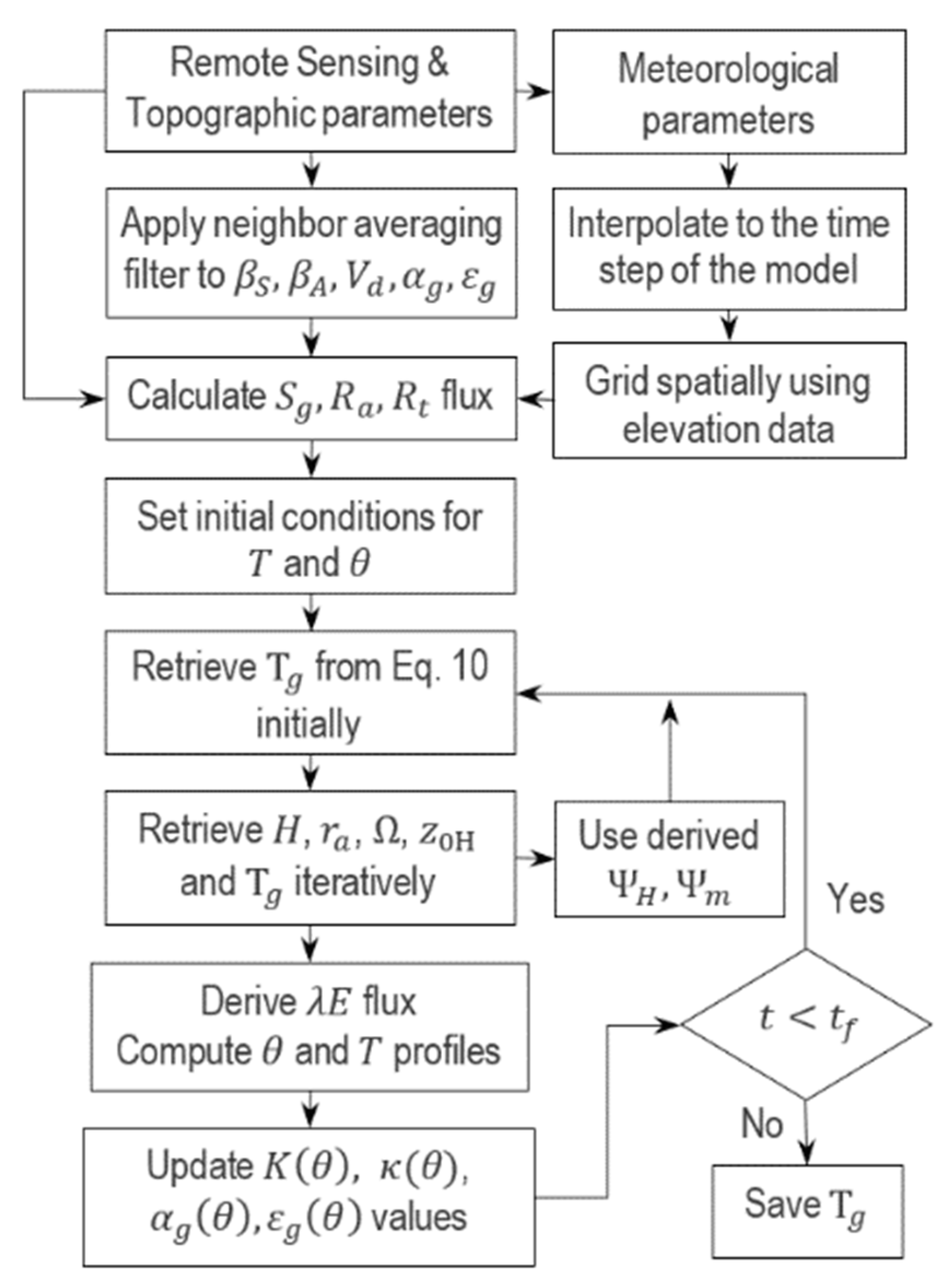
2.6. Numerical Solution of the Heat Flow Equation

The heat flow equation is converted into a set of ordinary differential equations of the form given in Equation (9) and solved using the Runge–Kutta 5th- and 6th-order methods:

$$\frac{dT}{dt}=\mathsf{\kappa }\left(\frac{T_{i+1}^n-{2T}_i^n+T_{i-1}^n}{{\mathsf{\Delta }z}^2}\right)$$

(9)

where $n$ and $i$ represent the time and spatial steps, respectively, and $\mathsf{\Delta }z$ $\left(\mathrm{m}\right)$ is the depth step size with $\mathsf{\kappa }$ being assumed to be a constant here (in practice, it is updated as a function of $\mathsf{\theta }$). The main advantage of this solution is that it is unconditionally stable allowing larger $\mathsf{∆}t$ steps to be used. The lower boundary is considered to be at some appropriate depth below which the diurnal heating wave is not reached (i.e., zero temperature gradient), which is usually at a depth between 1 and 3 m [27]. The upper boundary condition is obtained from Equation (2). By substituting Equations (3)–(9) into Equation (2) and rearranging the terms, a fourth-order polynomial for $T_g$ can be obtained, but since the solution of this nonlinear equation is computationally expensive, it is linearized using the first-order Taylor series expansion. As a consequence, the equation is reduced to:

$$T_g=\frac{\left(S_g+R_a+R_a^t+R_g^t+3{\mathsf{\epsilon }}_g\mathsf{\sigma }{T_a}^4+\frac{K{T}_1}{\mathsf{\Delta }z}\right)\left(1-\frac{\mathsf{\Omega }\mathsf{\Delta }}{\mathsf{\Delta }+\mathsf{\gamma }}\right)+\frac{{\mathsf{\rho }}_a{c}_m}{r_a} \left(T_a-\mathsf{\Omega }\frac{p_s\left(1-0.01R_H\right)}{\left(\mathsf{\Delta }+\mathsf{\gamma }\right)}\right)}{\frac{{\mathsf{\rho }}_a{c}_m}{r_a}+\left(\frac{K}{\mathsf{∆}z}+{4\mathsf{\epsilon }}_g\mathsf{\sigma }{T_a}^3\right)\left(1-\frac{\mathsf{\Delta }\mathsf{\Omega }}{\mathsf{\Delta }+\mathsf{\gamma }}\right)}$$

(10)

This equation runs at least 7× faster while introducing a maximum error of just 0.1 K in $T_g$ estimation, which is negligible when compared to other uncertainties.

The interval between the two boundaries is divided into i-computational layers of $\mathsf{∆}z$ thickness ($~$0.5–2.5 cm), with the possibility of increasing it exponentially downwards. In each iteration, $T_g$ is retrieved from Equation (10) and is used to update the subsurface temperature profile using Equation (9). By iterating for a predefined time (spin-up) period, a complete set of temperature values is achievable for each pixel as a function of time and depth, although the skin temperature values ($T_g$) at the end of the given interval are typically registered to be compared with measured temperature data (Figure 1).

2.7. Soil Water Flow Model

The volumetric soil water content ($\mathsf{\theta }$) is a key state variable governing the partitioning of available energy between latent and sensible heat fluxes [48]. Here, the flow of water in unsaturated soil is modeled using the linearized form of Richards’s equation:

$$\frac{\mathsf{\partial }\mathsf{\theta }}{\mathsf{\partial }t}=D_{\mathsf{\theta }}\frac{{\mathsf{\partial }}^2\mathsf{\theta }}{{\mathsf{\partial }z}^2}-k_h\frac{\mathsf{\partial }\mathsf{\theta }}{\mathsf{\partial }z}$$

(11a)

where $D_{\mathsf{\theta }}$ (${\mathrm{m}}^2\cdot {\mathrm{s}}^{-1}$) is the soil water diffusivity and $k_h$(${\mathrm{m}\cdot \mathrm{s}}^{-1}$) is a constant linearly related to $\mathsf{\theta }$ and $K_h$, the unsaturated soil hydraulic conductivity ($K_h={\mathsf{\theta }k}_h$). The analytical solution to Equation (11a) is given by Warrick [49]:

$${\mathsf{\varrho }}_n\left(Z_{\ast }\right)=\left\{\begin{array}{ll}\exp \hspace{0.17em}\left(\frac{-Z_{\ast }}{2}+\frac{T_{\ast }}{4}\right)F_{1}U\left(Z_{\ast },T_{\ast }\right)& n=1\\ \exp \hspace{0.17em}\left(\frac{-Z_{\ast }}{2}+\frac{T_{\ast }}{4}\right)F_{1}U\left(Z_{\ast },T_{\ast }\right)+{\displaystyle \sum _{i=2}^n}{(F}_i-F_{i-1}) U(Z_{\ast },[n-i+1]\mathsf{\Delta }{T}_{\ast })& n>1\end{array}\right.$$

(11b)

where $U$ is the solution for $(\mathsf{\theta }-{\mathsf{\theta }}_{\mathsf{\infty }})/{\mathsf{\theta }}_{\mathsf{\infty }}$ when $F\left(T_{\ast }\right)=1$ and $Z_{\ast }$, $T_{\mathrm{*}}$, $\mathsf{\varrho }$, and $F$ are normalized variables (-) as defined in Appendix C. Under clear-sky conditions, the net flux is assumed to be confined to the actual evaporation flux ($f=-E$) ($\mathrm{k}\mathrm{g}\cdot {\mathrm{m}}^{-2}\cdot {\mathrm{s}}^{-1}$). ${\mathsf{\theta }}_{\mathrm{\infty }}$ (${\mathrm{m}}^3\cdot {\mathrm{m}}^{-3}$) is the long-term average of soil moisture contents setting the lower boundary condition [50]. It is estimated from Warrick’s equation, as formulated in Appendix C.

Equation (11b) is applied to calculate the soil moisture distribution at any given depth during n-time steps of $\mathsf{\Delta }\mathrm{t}$ intervals. The evaporation flux ($-E$ in Equation (8a)) is fed into Equation (11b) to estimate the soil moisture profile and subsequently to calculate/update the $K(\mathsf{\theta })$ and $\mathsf{\kappa }(\mathsf{\theta })$ profiles alongside the ${\mathsf{\alpha }}_g\left(\mathsf{\theta }\right)$ and ${\mathsf{\epsilon }}_g\left(\mathsf{\theta }\right)$ parameters (see Figure 1). Considering that evaporation is a slow process, the soil moisture profile is updated every 20–30 min using the cumulative latent heat fluxes. The soil profile is assumed to be comprised of a uniform and homogeneous layer, and the soil water balance of each pixel is estimated independently. Soil water content is not permitted to drop below the residual (${\mathsf{\theta }}_r$) or exceed the saturated (${\mathsf{\theta }}_s$) soil water content. The water flow equations are only solved for pixels where ${\mathsf{\theta }}_s>0$. Over impermeable bedrocks, soil moisture is set to zero and thereby the heat transfer is calculated independent of $\mathsf{\theta }$. $D_{\mathsf{\theta }}$ is derived from the empirical soil hydraulic scheme described in Appendix D, using the average soil moisture profile. $K_h$ is treated as a constant (more on this in the Discussion section).

2.8. Iterative Retrieval of $r_a$ and $T_g$

Initially, the model assumes a neutral atmospheric condition at which ${\mathsf{\Psi }}_H={\mathsf{\Psi }}_m=0$ [23] and obtains an initial value for $r_a$ and subsequently for $\mathsf{\Omega }$ and $T_g$ using Equations (6b), (8c), and (10), respectively. $z_{0H}$ is initially assumed to be ${\frac{1}{7}z}_{0m}$ following Choudhury, Reginato, and Idso [51]. The obtained $H$ and $\mathsf{\zeta }$ (Equation (A1)) are then used to calculate new values for ${\mathsf{\Psi }}_H$ and ${\mathsf{\Psi }}_m$ (and $z_{0\mathrm{H}}$) using Equations (A3)–(A7). This process is repeated until a threshold level (e.g., $\mathsf{\Delta }H<1$) is satisfied (see Figure 1). The retrieved ${\mathsf{\Psi }}_m$ and ${\mathsf{\Psi }}_H$ are then used as initial values for the next time step to make the iterative process converge faster. In this way, the algorithm converges to the exact values after only one or two iterations.

The resulting $T_g$ is used to update the soil temperature profile and calculate the evaporation rate. The value of $\mathsf{\Delta }$ in Equation (8b) is calculated using the temperature of the previous time step ($T_g^{n-1}$) with an error of <1%, which can be treated as negligible.

2.9. Initial Conditions

The initial temperature profile of each pixel is assigned using a sinusoidal analytical model [52]:

$$T\left(z,t_0\right)=\overline{T_g}-\Delta T\exp \hspace{0.17em}\left(-\frac{z}{D_d}\right)\cos \hspace{0.17em}\left(\mathsf{\omega }{t}_0+{\mathrm{a}}_f-\frac{z}{D_d}\right)$$

(12)

where $\Delta T$ is the daily amplitude of the ground temperature, $D_d=\sqrt{\frac{2\mathsf{\kappa }}{\mathsf{\omega }}}$ is the damping depth ($\mathrm{m}$), $\mathsf{\omega }$ ($\mathrm{r}\mathrm{a}\mathrm{d}{\cdot \mathrm{s}}^{-1}$) is the angular frequency, ${\mathrm{a}}_{\mathrm{f}}$ ($\mathrm{r}\mathrm{a}\mathrm{d}$) is the phase angle of the time at which temperature is minimal, $z$ ($\mathrm{m}$) is the depth (positive downward), $\overline{T_g}$ is the mean daily surface temperature, and $\mathsf{\kappa }$ (${\mathrm{m}}^2\cdot {\mathrm{s}}^{-1}$) is thermal diffusivity, here assumed to remain constant with depth. When $T\left(0,t_0\right)$ is available from thermal remote sensing data, $\overline{T_g}$ could be obtained as $\overline{T_g}=T\left(0,t_0\right)+\mathsf{\Delta }\mathrm{T}\cos \hspace{0.17em}\left(\mathsf{\omega }{t}_0+{\mathrm{a}}_f\right)$. $\mathsf{\Delta }T$ could be approximated by either a pair of daytime and nighttime temperature data or by assuming it to be equivalent to the daily air temperature amplitude. As is discussed in Section 6, a spin-up period of several days would then be required to obtain realistic initial conditions.

For the soil moisture, the initial profile derived from the Warrick equation is combined with a simple moisture profile obtained by linear interpolation between $\mathsf{\theta }$ at the surface and ${\mathsf{\theta }}_{\mathrm{\infty }}$ at the bottom of the profile.

3. Parameter Estimation

3.1. Meteorological Parameters

Assuming that the atmospheric forcing is uniform across a given area at each moment, any observed variations could be presumed to arise from topographic elevation. Such conditions can then be represented by a single weather station located within or close to the study area. The meteorological parameters comprising air temperature ($T_a$), air pressure ($p_a$), and relative humidity ($R_H$) together with the calculated air density (${\mathsf{\rho }}_a$), are initially interpolated to a $\mathsf{\Delta }\mathrm{t}$ time step using the shape-preserving cubic spline method and are then spatially gridded using elevation data (Figure 1).

The power law ($\upsilon \left(Z\right)={\upsilon }_2{\left(\frac{Z}{Z_0}\right)}^a$, where $0.11<a\le 0.14$ is the exponential value for the vertical wind profile and $Z_0$ is the altitude of the weather station, is used to correct for the vertical profile of the wind speed (${\upsilon }_2$) against topographic height $Z$ ($\mathrm{m}$). This simplified model applies only to hilly terrains, and over complex topography it would be erroneous. Accurate and reliable prediction of the wind flow fields over complex terrains demands solving the Navier–Stokes equations using wind and topographic data (e.g., [53]), the discussion of which is beyond the scope of this article. Nonetheless, SKinTES has the capability of incorporating wind maps derived from specialist programs like WAsP (Roskilde, Denmark) into the analysis.

3.2. Remote Sensing Parameters

The topographic data and derived products (i.e., ${\mathsf{\beta }}_S$, ${\mathsf{\beta }}_A$, $V_d$, and $C_t$) are obtained from a high-spatial-resolution DEM. The remaining parameters are derived from remote sensing data as outlined below. Considering that each dataset comes from different sources/sensors, meticulous orthorectification is required (and applied) to ensure that they are spatially closely aligned with the underlying topography.

3.2.1. Broadband Surface Albedo

The broadband surface albedo in the range between $0.3 \mathrm{a}\mathrm{n}\mathrm{d} 3.0 \mathsf{\mu }\mathrm{m}$ is derived by applying narrow-to-broadband conversion coefficients to the corresponding satellite remote sensing data [54]. The narrow bands ($R_{\mathsf{\lambda }}$) (-) are initially corrected for topographic/illumination effect using the formulation provided in Richter [55]:

$$R_{\mathsf{\lambda }}^{\prime }=R_{\mathsf{\lambda }}\left(\frac{\cos \hspace{0.17em}{\mathsf{\phi }}_z}{\cos \hspace{0.17em}{\mathsf{\phi }}_z^{\prime }}\right){\left(\frac{\mathit{cos}\hspace{0.17em}{\mathsf{\phi }}_z^{\prime }}{\mathit{cos}\hspace{0.17em}{\mathsf{\phi }}_t}\right)}^M$$

(13)

where $\cos \hspace{0.17em}{\mathsf{\phi }}_z^{\prime }$ is the solar incident angle calculated from Equation (3c) for the image acquisition time, ${\mathsf{\phi }}_z$ is the corresponding solar zenith angle, ${\mathsf{\phi }}_t$ is defined as a function of ${\mathsf{\phi }}_z$, and $M$ (-) is an empirical parameter here set to 0.5 for non-vegetated terrain.

In dry regions, the volumetric soil water content ($\mathsf{\theta }$) has little variation over short time periods, and accordingly, ${\mathsf{\alpha }}_g$ can be treated independently of $\mathsf{\theta }$. Otherwise, their relationship is given by [56]:

$${\mathsf{\alpha }}_g\left(\mathsf{\theta }\right)={\mathsf{\alpha }}_d\exp \hspace{0.17em}\left({-a}_1\mathsf{\theta }\right)$$

(14)

where ${\mathsf{\alpha }}_d$ is dry surface albedo derived from topographic corrected data, and $a_1$ is an empirical coefficient determined as the slope of $-\mathrm{l}\mathrm{n}\left(\frac{{\mathsf{\alpha }}_g\left({\mathsf{\theta }}_0\right)}{{\mathsf{\alpha }}_d}\right)$ against ${\mathsf{\theta }}_0$, which is the soil moisture content at $t=0$.

The effect of the diurnal cycle on surface albedo is modeled according to Equation (15), which is a variant of the Dickinson model [57] here modified to incorporate albedo at the time of image acquisition (see Appendix E for the derivation):

$${\mathsf{\alpha }}_g\left(\mathsf{\mu }\right)={\mathsf{\alpha }}_g\frac{1+2d{\mathsf{\mu }}_0}{1+2d\mathsf{\mu }}$$

(15)

where $\mathsf{\mu }$ is the cosine of the solar zenith angle ($\cos \hspace{0.17em}{\mathsf{\phi }}_z$), ${\mathsf{\alpha }}_g$ is the satellite-derived surface albedo at the zenith angle ${\mathsf{\mu }}_0$ (corresponding to image acquisition time), and $d$ (-) is a constant here set to 0.15 according to Wang, et al. [58]. Equation (15) only applies to flat surfaces. For rugged terrains, $\mathsf{\mu }$ should be substituted with $\cos \hspace{0.17em}{\mathsf{\phi }}_z^{\prime }$ obtained from Equation (3c).

3.2.2. Broadband Surface Emissivity

The broadband surface emissivity (${\mathsf{\epsilon }}_g$) in the range between 8 and 13.5 μm is derived from narrowband emissivities following a linear conversion [59]. Surface emissivity is known to be strongly affected by soil moisture content ($\mathsf{\theta }$), the effect of which could be modeled using a logarithmic equation of the following form [60]:

$${\mathsf{\epsilon }}_g\left(\mathsf{\theta }\right)=b_0+b_1\mathsf{\theta }+b_2\ln \hspace{0.17em}\left(\mathsf{\theta }\right)$$

(16)

where $b_i$ are regression coefficients. $b_0$ could be determined by time series analysis of emissivity data during dry seasons when $\mathsf{\theta }\approx 0$. For broadband emissivity, $b_1$ is set to zero. Thus, given the remotely sensed soil moisture content (${\mathsf{\theta }}_0$) and broadband emissivity (${\mathsf{\epsilon }}_{g_0}$) at $t=0$, $b_2$ could be estimated for each image pixel as $b_2=\frac{{\mathsf{\epsilon }}_{g_0}-b_0}{\mathrm{l}\mathrm{n}\left({\mathsf{\theta }}_0\right)}$.

3.2.3. Soil Moisture Content

The thermal–optical trapezoid model described in Sadeghi, et al. [61] is used to estimate the volumetric soil moisture contents (${\mathrm{m}}^3\cdot {\mathrm{m}}^{-3}$). The $\mathsf{\theta }$ provided by this approach is known to be representative of the uppermost layer (i.e., 0–5 cm). The moisture contents of the lower layers are estimated/updated using the hydrological scheme described in Section 2.7.

3.2.4. Soil and Rock Thermal Properties

The surface thermal conductivity, $K\left(\mathsf{\theta }\right)$, is calculated as:

$$K\left(\mathsf{\theta }\right)={K_{dry}+K}_e\left(K_{sat}-K_{dry}\right)$$

(17a)

where $K_e$ (-) is the degree of saturation, and $K_{sat}$ and $K_{dry}$ (${\mathrm{W}\cdot \mathrm{m}}^{-1}{\cdot \mathrm{K}}^{-1}$) are the dry and saturated thermal heat conductivities derived from a modified form of the Johansen [62] model:

$$K_{sat}={\left(k_s\right)}^{1-{\mathsf{\theta }}_s}{k_w}^{{\mathsf{\theta }}_s}$$

(17b)

where ${\mathsf{\theta }}_s$ (${\mathrm{m}}^3\cdot {\mathrm{m}}^{-3}$) is the saturated volumetric soil water content, $k_w$ is the thermal conductivity of water (taken as $0.57{\mathrm{W}\cdot \mathrm{m}}^{-1}{\cdot \mathrm{K}}^{-1}$), and $k_s$ is that of solid particles assessed by using the generalized geometric mean method [63]:

$$k_s={\prod }_j{k}_{m_j}^{x_j} \mathrm{with} {\sum }_j{x}_j=1$$

(17c)

where $k_m$ is the thermal conductivity of mineral/rock $j$ with $x$ volumetric proportion, approximated here using the mineral abundance maps derived from topographically corrected multispectral remote sensing data (see the details in Section 4.2). A similar methodology, based on mineral maps, is used to calculate $C_s$ (${\mathrm{M}\mathrm{J}\cdot \mathrm{m}}^{-3}\cdot {\mathrm{K}}^{-1}$), the volumetric heat capacity of solid rocks.

For impermeable bedrock, $K_{dry}$ is assumed to be equal to $K_s$. For permeable rocks and soil media, it is given by:

$$K_{dry}=\frac{0.135\left(1-{\mathsf{\theta }}_s\right){\mathsf{\rho }}_s+64.7}{{\mathsf{\rho }}_s-0.947\left(1-{\mathsf{\theta }}_s\right){\mathsf{\rho }}_s}$$

(17d)

$${\mathsf{\rho }}_s={\sum }_j{\mathsf{\rho }}_{m_j}^{x_j} \mathrm{with} {\sum }_j{x}_j=1$$

(17e)

where ${\mathsf{\rho }}_m$ ($\mathrm{k}\mathrm{g}\cdot {\mathrm{m}}^{-3}$) is the mean bulk density of rock type $j$ with $x$ volumetric proportion.

3.2.5. Surface Roughness Length

The surface roughness length ($z_{0m}$) of bare surfaces typically spans several orders of magnitude, ranging from 0.0001 to 0.01 m. Here, $z_{0m}$ is parametrized using remote sensing land cover analysis guided by geological knowledge. In this approach, the study area is partitioned into N segments using supervised classification techniques and subsequently, a representative $z_{0m}$ value is assigned to each segment by considering the characteristics of the surface and a set of guidelines compiled from the literature for the roughness length of bare surfaces. In rugged terrains, the assigned values are further adjusted for the topographic slope effect (${\mathsf{\beta }}_S$, in degree) using a simple function proposed by Allen, Tasumi, and Trezza [23]:

$$z_{0m}={z^{\prime }}_{0m}\left(1+\frac{{\mathsf{\beta }}_S-5}{20}\right)$$

(18)

4. Numerical Experimentation

4.1. Study Sites

To give credibility to the developed model, its performance was tested over two different landscapes at two different spatial scales under a range of soil moisture, elevation, and meteorological conditions. This includes the Tongyu observation site located in the semiarid region of NE China ($44°{25}^{\prime }\mathrm{N},122°{52}^{\prime }\mathrm{E}$) at an elevation of 184 m [33] and the Qom area in Central Iran spanning between $34°{36}^{\prime }$ and $34°{42}^{\prime }$N, and $50°{40}^{\prime }$ and $50°{47}^{\prime }$E at elevations varying from 930 to 1600 m (see Figure 8a). The Tongyu site comprises point-scale observational data collected in 2005 and provided to us for the current study. It includes high-temporal-resolution meteorological data and soil temperature measurements at depths of 0, 2, 5, 10, 20, 50, and 80 cm recorded at half-hour intervals. This dataset was used to evaluate the model’s overall performance in simulating the diurnal surface temperature and energy flux densities, find the optimum settings for the step sizes, spin-up period, and initial conditions, and perform a sensitivity analysis. The Qom area, on the other hand, is comprised of a rugged topography (as depicted in Figure 8a) with a complex geologic setting characterized by a diverse range of sedimentary rocks, including sandstones, limestones, shales, and alluviums (as shown in Figure 8b) and ruled by an arid to semiarid climate. This site was covered by ASTER thermal remote sensing data.

4.2. Model Setup

The parameters of the first experiment are listed in

Table 1. Surface parameters of the Tongyu cropland station (after Xia [33]).

Model Parameter	Value
Surface albedo	0.28
Surface emissivity	0.964
Soil porosity	0.415
Sand (%)	58
Clay (%)	35
Saturation hydraulic conductivity (m2$\cdot$s−1)	7.11 $\times$ 10−6
Aerodynamic roughness length (m)	0.006

. The simulation was carried out for an eight-day period from 23 to 30 April 2005, which falls within the dry season of early spring with no vegetation cover (i.e., bare soil). The simulation in this study was synchronized with the timing of satellite data overpass (e.g., 10:30 a.m. to 10:30 p.m.). The measured surface temperature in conjunction with Equation (12) was used to set the initial temperature profile. The soil moisture profile was initialized by running the Warrick equation for 40 h and combining the results with a linearly interpolated moisture content between $\mathsf{\theta }$ and ${\mathsf{\theta }}_{\mathsf{\infty }}$. A spin-up period of six days was used to initialize the simulation.

The second study area was covered by a pair of day- and nighttime ASTER (Advanced Spaceborne Thermal Emission and Reflection Radiometer) thermal remote sensing satellite data on 10 and 15 August 2020. We derived surface kinetic temperature and surface emissivity data from AST08 and AST05 standard products, respectively (Figure 8c), using the GDAS model for the atmospheric moisture profile (earthdata.nasa.gov accessed on 3 October 2023). The datasets were initially orthorectified and their inherent stripping noise was removed in the frequency domain using the Fast Fourier Transform (FFT). The broadband surface emissivity was calculated following the conversion coefficients offered by Cheng, Liang, Yao, and Zhang [59] (i.e., ${\mathsf{\epsilon }}_g=0.025{\mathsf{\epsilon }}_{10}+0.057{\mathsf{\epsilon }}_{11}+0.237{\mathsf{\epsilon }}_{12}+0.333{\mathsf{\epsilon }}_{13}+0.146{\mathsf{\epsilon }}_{14}+0.197$, where ${\mathsf{\epsilon }}_{\mathrm{i}}$ are emissivities at channels 10–14). The plot of NDVI from VNIR bands against kinetic surface temperature was used to estimate the soil moisture content at the time of image acquisition. Given that the ASTER SWIR detector was no longer functional, the land surface broadband albedo was calculated from a topographically corrected Landsat-8 Level-2 data product acquired on 9 August 2020 by the following equation: ${\mathsf{\alpha }}_g=0.356a_2+0.130a_4+0.373a_5+0.085a_6+0.072a_7-0.0018$, where ${\mathsf{\alpha }}_i$ is the narrowband spectral reflectance of the band “i” of the instrument [54]. The multispectral datasets in combination with a 1:100 K geologic map and some field observations were used to assign the surface roughness length values. For this aim, the scene was classified into four land covers (i.e., sandstones, limestones, shales/marls, and alluviums; Figure 8b) and a $z_{0m}$ value ranging between 0.0015 and 0.02 m was assigned to each cover type. The daytime emissivity data were used to estimate the quartz content of the surface constituents. The abundance maps of clay, limestone, and sandstone were derived from the ASTER-SWIR bands [64] and the Landsat-8 Level-2 product, respectively. The clay and quartz abundance maps were used to calculate soil hydraulic parameters according to Appendix D. The thermal properties of rocks were mapped using Equations (17b)–(17e) and the values listed in

Table 2. Values of thermal conductivity (${\mathrm{k}}_{\mathrm{m}}$), mean density (${\mathsf{\rho }}_{\mathrm{m}}$), and volumetric heat capacity of solids (${\mathrm{C}}_{\mathrm{s}}$) used to map the rock thermal properties of the Qom study area.

Rock Type	${\mathbf{k}}_{\mathbf{m}}$$({\mathbf{W}\cdot \mathbf{m}}^{-1}\cdot {\mathbf{K}}^{-1}$)	${\mathsf{\rho }}_{\mathbf{m}}$$(\mathbf{k}\mathbf{g}{\cdot \mathbf{m}}^{-3}$)	${\mathbf{C}}_{\mathbf{s}}$$(\mathbf{M}\mathbf{J}{.\mathbf{m}}^{-3}\cdot {\mathbf{K}}^{-1}$)
Quartz	7.7	2650	-
Sandstone	3.0	2800	2.8
Limestone	2.5	2700	2.4
Shale	2.0	2650	2.5
Alluvium	2.0	2700	2.0

for thermal conductivity, mean density, and heat capacity. Elevation data at a 30 m spatial resolution were derived from the ALOS DEM (JAXA, Japan). The sky view factor was calculated following the procedure described in Zakšek, Oštir, and Kokalj [37], which involves a search radius of 20 pixels and 32 search directions. Initial conditions were derived from the pair of temperature datasets using the approach described in Section 2.9. The rest of the parameters were estimated according to the methods detailed in Section 3. In the end, raster inputs were aggregated to a 90 m pixel size to align with the measured temperature data. A six-day period, from 10 to 15 August 2020, was used to spin up the model. Historical meteorological data were obtained from the Qom weather station at three-hour intervals. Since the simulation time coincided with the dry season, no corrections were applied to ${\mathsf{\epsilon }}_g$ and ${\mathsf{\alpha }}_g$ for soil moisture contents.

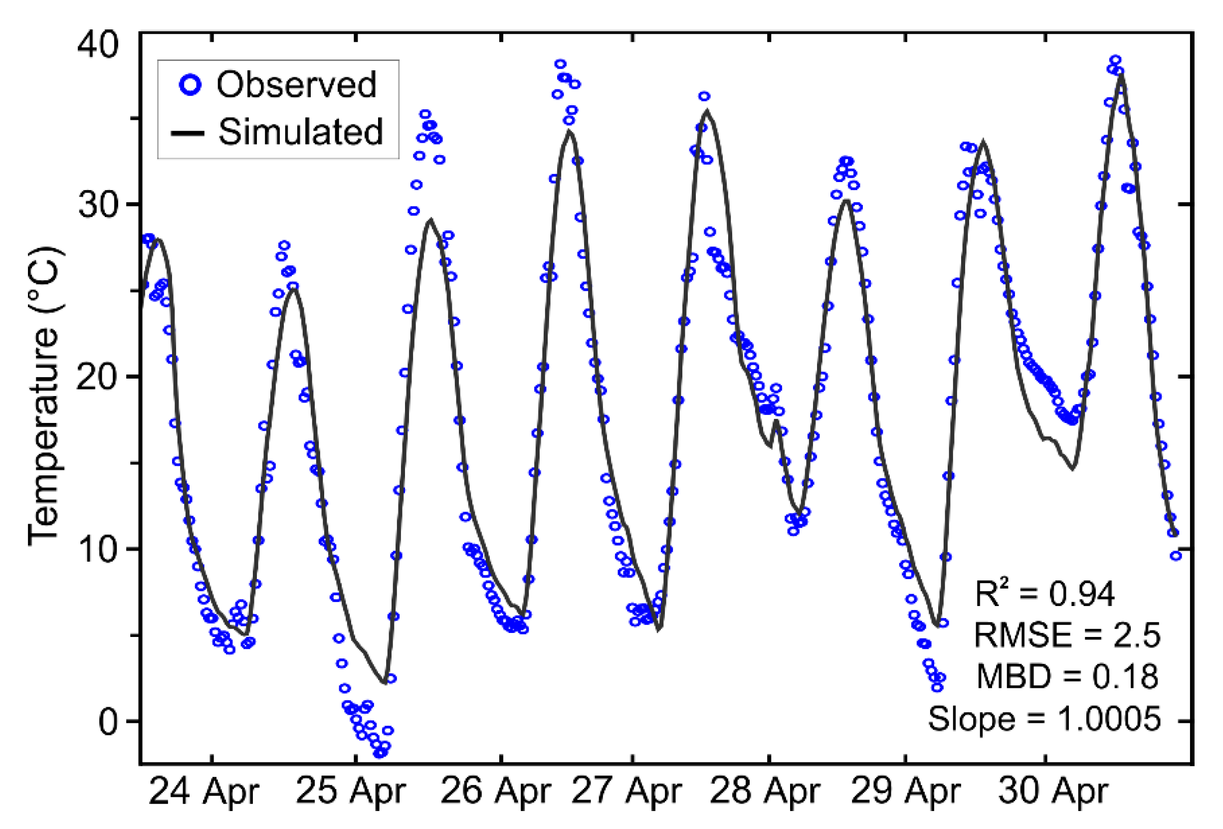
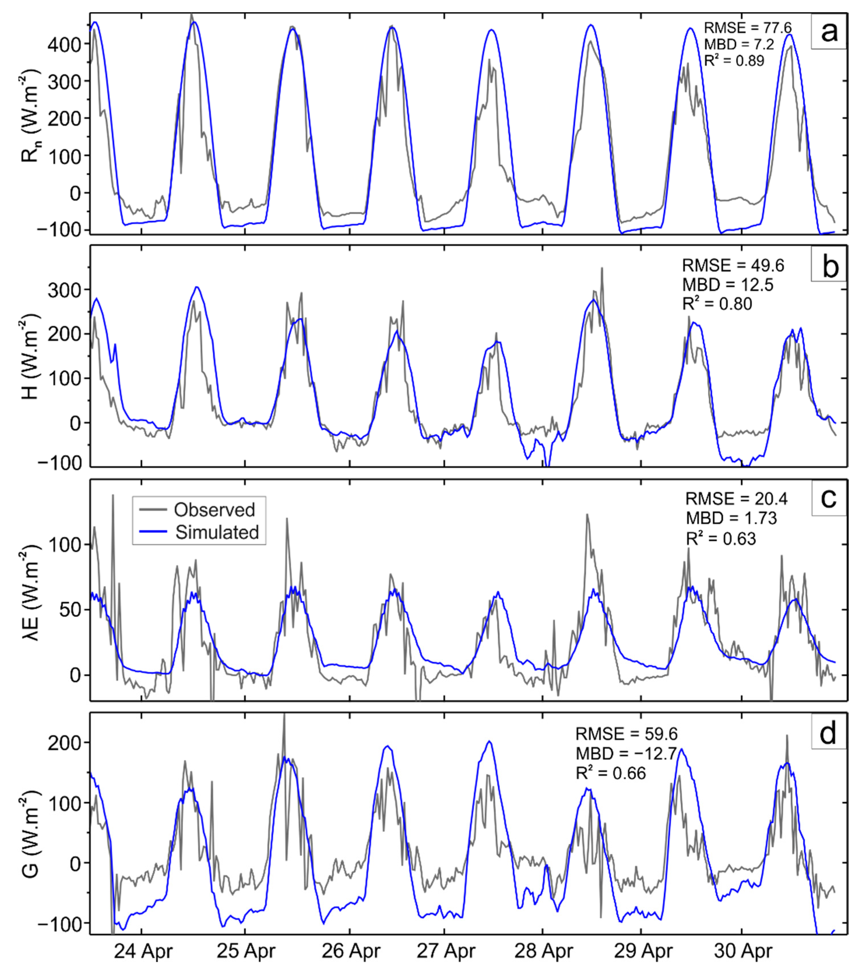
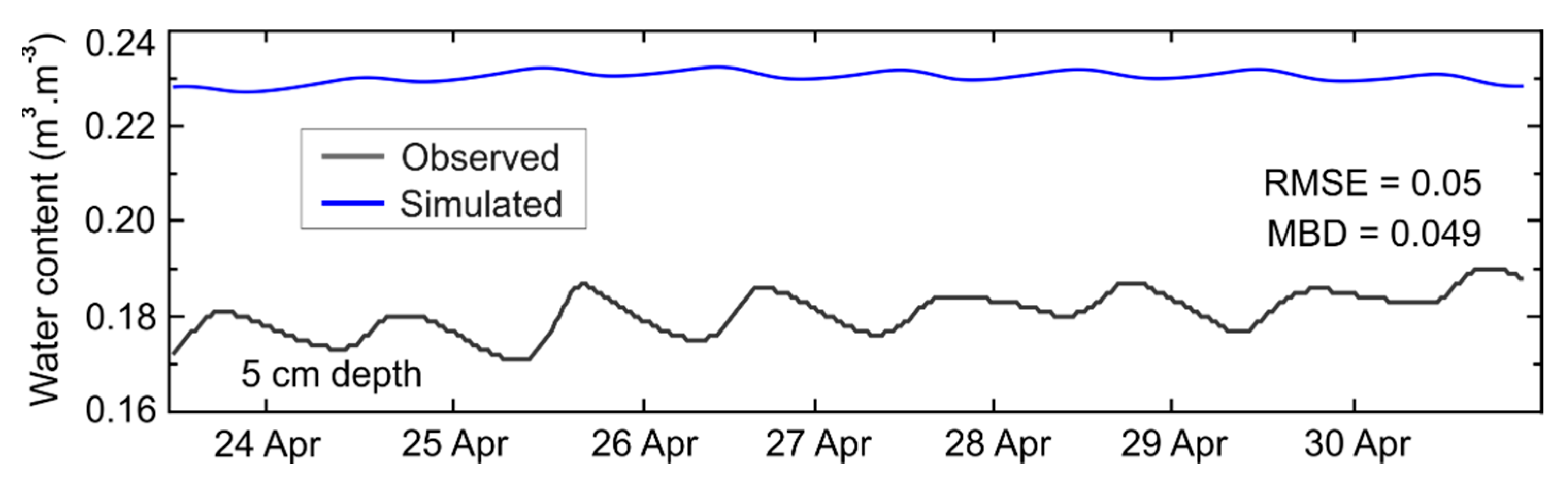
4.3. Model Evaluation

The model’s performance was evaluated using several statistical metrics, including the root mean square error (RMSE) and the mean bias deviation (MBD). These metrics help identify any systematic under- or overestimation tendencies in the model when compared to measured data. A linear regression analysis was also conducted on the paired data, with the regression line forced through the origin. The coefficient of determination, R², was used to evaluate the variance of the model. The absolute temperature difference between the simulated and measured data at the last time step was used as an additional metric for model performance evaluation.

4.4. Sensitivity Analysis

A sensitivity analysis was conducted to evaluate the impact of input parameter uncertainties on model performance. A total of 19 parameters were selected and each was permitted to vary by ±25% around its base value, with the three exceptions of $D_{\mathsf{\theta }}$, $k_h$, and $Z_{0m}$, which were allowed to vary one order of magnitude around their base values. The sensitivity of the model was assessed by calculating the RMSE and MBD for the increased ($O_{+}$) and decreased ($O_{-}$) outputs against the output from the base values.

5. Results

Figure 2 shows a comparison of simulated and observed surface temperatures ($T_g$) at the Tongyu station during a one-week period from 23 to 30 April 2005. The two datasets agree with each other to within 2.5 °C, exhibiting an MBD of 0.18 °C, R² of 0.94, and a regression slope of 1.0005. The largest discrepancies tend to occur around the daily maximums and minimums and the temperature disparity in the interval between them is minimal. Importantly, at the last time step, the temperature difference remains below 0.98 °C.

The observed and simulated energy fluxes for the same period accompanied by statistical errors are depicted in Figure 3. For the net radiation (Figure 3a), the RMSE and MBD are equal to 77.6 and 7.2 $\mathrm{W}{\cdot \mathrm{m}}^{-2}$, respectively, with 89% of the variance being described by the model. The bias, however, is not uniformly distributed throughout the simulation period, with some days (e.g., 25 April) showing excellent agreement with the observations. The most significant discrepancies tend to occur at night, when $R_n$ is largely underestimated.

The volumetric soil water content at 5 cm depth is systematically overestimated by the model (Figure 4). However, its difference with the observed values remains <0.05 ${\mathrm{m}}^3{\cdot \mathrm{m}}^{-3}$, as evidenced by an RMSE and MBD of 0.05 and 0.049 ${\mathrm{m}}^3{\cdot \mathrm{m}}^{-3}$, respectively. The model-simulated data also show a lower amplitude and a phase shift in the oscillations when compared to the measured data. The corresponding soil moisture profile along the depth, though not shown, closely aligns with the observations, with an RMSE of 0.018 and MBD of $-$0.004 ${\mathrm{m}}^3{\cdot \mathrm{m}}^{-3}$.

Although the update time interval of the soil moisture content (see Section 2.7) has no noticeable effect on the overall accuracy of the retrieved $\mathsf{\theta }$ (and $T_g$) values, it was found to have profound impacts on the overall processing time. Accordingly, for the sake of efficiency, the soil moisture profile was set to update every 20–30 min. The effect of step sizes on the overall performance of the model is summarized in Figure 5. It indicates that time spacing could be increased up to 180 s at the expense of a slight decline in the overall accuracy, though at $\mathsf{\Delta }t=240 \mathrm{s}$ the model starts to give unrealistic results. According to Figure 5, the optimal node spacing and time intervals fall within the ranges of 1.5–2.5 cm and 60–90 s, respectively. The optimal lower boundary condition was determined to be 1.0 m below the surface.

We tested to see whether the temporal resolution of meteorological data affects the accuracy of $T_g$ predictions and realized that by decreasing the interval from half an hour to three hours, the RMSE of the prediction remains almost unchanged. At four-hour intervals, however, we observed a 10% increase in RMSE and a 25% increase in MBD. Furthermore, by using the diurnal air temperature maxima/minima as inputs to Equation (12), the results closely resembled those depicted in Figure 2, with differences of <0.1 °C. By contrast, the spin-up period was found to profoundly affect the results, particularly the simulated temperature at the last time step (Figure 6). A decrease in the spin-up period was found to progressively increase the relative error such that at a spin-up rate of 12 h, the error reached 90% of the initial setting (i.e., spin-up rate of 13.5 days).

The sensitivity analysis results, as summarized in Figure 7, indicate that $T_a$, $\mathsf{\theta }$, ${\mathsf{\alpha }}_g$, $p_a$, and ${\mathsf{\epsilon }}_g$ are the principal sensitive parameters of the model when simulating the diurnal surface temperature pattern followed by the $Z_{0m}$ and ${\mathsf{\omega }}_0$ parameters (Figure 7b). By contrast, the simulated temperature at the last time step is mainly sensitive to ${ T}_a$ and to a lesser extent $\mathsf{\theta }$, ${\mathsf{\epsilon }}_g$, $K_{sat}$, and ${\mathsf{\omega }}_0$ (Figure 7a). Amongst the input parameters, $\mathsf{\theta }$, $K_{dry}$, and $Z_{0m}$ appear to be more sensitive to overestimations, whereas $T_a$, $p_a$, $K_{sat}$, and ${\mathsf{\alpha }}_g$ show sensitivity to both under- and overestimations. ${\mathsf{\epsilon }}_g$ show to be highly sensitive to underestimation. Notably, the model (explicitly Equation (11b)) has no sensitivity to the $k_h$ value, and thus it is treated as a constant ($=1.15741\times {10}^{-9} \mathrm{m}{\cdot \mathrm{s}}^{-1}$).

Figure 8c,d show the measured and model-simulated land surface temperatures across the Qom study area. The simulated temperature map (Figure 8d) appears to reproduce the spatial patterns of the ASTER-derived LST in large parts of the area. The RMSE and MBD between the paired data are equal to 1.74 and $-$0.35 °C, respectively. The simulated skin temperature accounts for 19% of the variance of the remotely sensed kinetic temperature data. The largest discrepancies are found over the north-facing slopes (depicted by U₁ in Figure 8d) and alluvial fans towards the south (U₂ in Figure 8d) over which the temperature is largely underestimated. By contrast, the temperatures in small patches toward the NE and central zones appear to be overestimated (O in Figure 8d). It is worth noting that while the remote sensing LST data of Figure 8c are used as a reference, there appears to be a dependency between the range and quality of temperature data and the applied atmospheric correction methodology, with MODIS-based atmospherically corrected images appearing to retain relatively poor quality.

6. Discussion

Under clear-sky conditions, there is an uncertainty of about 25 $\mathrm{W}\cdot {\mathrm{m}}^{-2}$ in the calculation of $R_n$ (Figure 3a) attributed to Prata’s model (${\mathsf{\epsilon }}_a$ in Equation (5a)) [65]. Given the low uncertainty of Yang’s model in estimating $S_g$ flux, measured to be <10 $\mathrm{W}\cdot {\mathrm{m}}^{-2}$ [35,40], and considering the systematic underestimation of $R_a$ by Prata’s model over the Tongyu site (indicated by MBD = $-$46.9 and RMSE = 54.5 $\mathrm{W}\cdot {\mathrm{m}}^{-2}$), it becomes evident that the main source of uncertainty in $R_n$ calculation (Figure 3a) is related to cloud effects. Under cloudy conditions, the overestimation of solar radiation during daytime is partly compensated by the underestimation of the downwelling longwave radiation [42]. During the night, however, clouds introduce a large discrepancy between the modeled and observed net radiation (Figure 3a). So, even the diurnal corrections of sky emissivity (Section 2.2) fail to alleviate the shortcomings of the model. Overall, Prata’s model appears to consistently underestimate $R_a$ flux by between 8 and 30%.

To understand the extent to which a clear sky model like SKinTES is affected by clouds, the ratio of downwelling longwave radiation in a cloudy sky ($R_{aC}$) to that of a clear sky ($R_a)$ was calculated ($\frac{R_{aC}}{R_a}=1+q_c{N}^2$, where $0.04\le q_c\le 0.25$ is an empirical constant dependent on cloud type/elevation and $0\le N\le 1$ is the cloudiness [42]) and plotted against cloudiness for different cloud types (Figure 9). The graph indicates that a cloudiness level up to 0.4 results in <4% (equivalent to <12 $\mathrm{W}{\cdot \mathrm{m}}^{-2}$) increase in $R_a$ flux, regardless of the cloud type. This signifies that the SKinTES model would not be confined to perfectly clear skies and that it could be confidently applied to partly cloudy conditions. Under a fully cloudy sky, however, $R_a$ would be underestimated by more than 25% using Prata’s model, which closely matches the 30% level observed in the Tongyu site. On the other hand, the presence of small cloud patches casting shadows over a pixel has a negligible effect on both the global solar radiation ($S_g$) and $T_g$ simulations, because blocking the direct sunbeam at around midday for up to five minutes (to mimic the effects of passing clouds) resulted in a mere 0.05 °C change in the RMSE of the retrieved $T_g$ values shown in Figure 6. This is important because, in practice, finding a temporal window with completely cloud-free skies to spin up the model is often challenging, if not impossible. It is important to note that since clear skies are a prerequisite for successful remote sensing data acquisition for geological applications, such problems could be largely circumvented by careful data selection/acquisition.

The discrepancy between the simulated and measured $T_g$ in Figure 2 is largely related to inaccuracies in estimating the ground heat flux, which in turn, is caused by systematic underestimation of $R_n$ flux (Figure 3a). During the night, the dominance of the ground heat flux in the energy balance directly affects the net longwave radiations, and thereby, the retrieved $T_g$ values (Figure 2) [26,34,66]. This is why evaporation maintained a positive rate throughout the nights (Figure 3c). By contrast, the underestimation of $T_g$ during midday hours (Figure 2) is likely related to the overestimation of soil moisture content (Figure 4).

The shift in the frequency of the soil moisture profile (Figure 4) can be attributed to positive evaporation rates at night and likely to the way $D_{\mathsf{\theta }}$ is calculated/updated under the assumption of a homogeneous soil profile, which neglects across-layer water flow [33,48]. The systematic overestimation of soil moisture content, however, is mostly due to an unrealistic initial condition (see Section 2.9), because by setting the initial conditions appropriately using the measured $\mathsf{\theta }$, for instance, the RMSE of Figure 4 declines to 0.02 ${\mathrm{m}}^3{\cdot \mathrm{m}}^{-3}$. This shows that coupling the Warrick equation with an advanced analytical model (e.g., the principle of maximum entropy) to set a more realistic initial condition can effectively predict the soil moisture dynamics in both space and time [50]. Similarly, the relatively accurate estimate of the latent heat flux (Figure 3c) indicates that the evaporation coefficient ($\mathsf{\Omega }$ function) effectively constrains potential evaporation [47] and that the Penman–Monteith equation is viable to calculate the diurnal latent heat of evaporation over bare surfaces, provided that it is coupled with the physically correct formula for Δ (Equation (8b) and an elaborate water budget [44,46].

The underestimation of $T_g$ over the alluvial deposits in the Qom area (U₂ in Figure 8d) is likely related to the cooling effect of evaporation caused by unusually high soil moisture contents (i.e., $0.18 {\mathrm{m}}^3{\cdot \mathrm{m}}^{-3}$) derived from the trapezoid method, as well as the tendency of the Warrick equation to overestimate soil moisture content under dry conditions [50] (Figure 4). In geologically heterogeneous and sparsely vegetated regions, the thermal–optical relationship often deviates from the norm, leading to higher uncertainties in soil moisture estimations. In such cases, the optical trapezoid model proposed by Sadeghi, Babaeian, Tuller and Jones [61] could provide an alternative means of mapping soil moisture contents. Furthermore, arid and semi-arid regions typically feature a very shallow soil layer underlain by impermeable bedrock among which the moisture flux is zero [66]. Ignoring this vertical heterogeneity has been identified as a significant source of errors in LSMs [48]. To account for this phenomenon, a multilayered soil model is planned for future incorporation into the SKinTES model.

On the other hand, the underestimation of $T_g$ over the north-facing slopes (U₁ in Figure 8d) can be attributed mostly to unrealistic initial conditions arising from the topographic slope and aspect of the daytime temperature data used to set Equation (12), although multiple reflections between the ground and sky (not yet accounted for in the model; Equation (3a)) may play a role. It is important to note that modeling the ground temperature profile correctly is crucial to avoid underestimating the land surface temperature [66]. While a longer spin-up period could potentially alleviate this issue (Figure 6), it is not a feasible option here due to computational expenses. In the current design, the spin-up period of SKinTES is confined to the interval between pairs of day- and nighttime temperature data. Over flat areas, a spin-up period of >60 h can yield reliable results (Figure 6). However, achieving more realistic initial conditions over north-facing slopes requires a tailored solution, which is currently under development. It is worth noting that the model’s relative insensitivity to the temporal resolution of meteorological data suggests that by adopting a proper interpolation technique (e.g., shape-preserving cubic spline), the impact of low temporal resolution in meteorological datasets can be largely circumvented during numerical modeling (e.g., [34]).

Over dry regions with limited soil water content, the surface temperature becomes highly sensitive to thermal inertia, and this parameter significantly influences the spatial distribution of temperature patterns [66,67]. The overestimation of temperature in Figure 8d is likely partly related to inaccuracies in the parameterization of surface thermal properties, particularly $K_{\mathrm{s}\mathrm{a}\mathrm{t}}$ values (Figure 7).

In geological applications, a low uncertainty is required for the model to effectively detect subtle subsurface temperature anomalies. Typically, uncertainties in the prediction of LST stem from two major sources: (i) uncertainty in input parameters, and (ii) model uncertainty due to simplified underlying assumptions [21]. When accurate estimates of incoming fluxes are used (equivalent to using measured fluxes as input to SKinTES), the model’s uncertainty was observed to reduce to <1.8 °C for the diurnal temperature profile and <0.5 °C for the temperature at the last time step (Figure 5). This level of uncertainty likely represents the inherent cumulative error of the model related to model realization. This is comparable to the detection limit of other similar methodologies, which has been reported to range between 2 °C and 5 °C [19,32].

Among the sensitive input parameters identified in Figure 7, surface albedo (${\mathsf{\alpha }}_g$) and emissivity (${\mathsf{\epsilon }}_g$) can be estimated with an accuracy greater than ±0.05 absolute units following the procedures described in Section 3.2. However, it is crucial to adjust these parameters for soil moisture content, because in dry regions such as the Qom, as an example, emissivity can vary by up to 0.04 units between dry and wet seasons. Failing to account for this variation could lead to a 3 °C uncertainty in $T_g$ estimation, a figure that exceeds the 1–2 °C variability reported in the study by Malbéteau, Merlin, Gascoin, Gastellu, Mattar, Olivera-Guerra, Khabba, and Jarlan [20].

The main challenge in simulating surface temperature patterns, however, is to generate a spatially distributed air temperature ($T_a$) with adequate accuracy (Figure 7). Under spatially uniform meteorological conditions, the predominant source of spatial variability in $T_a$ is the air temperature lapse rate, which is known to exhibit significant variability during diurnal and seasonal cycles, with the lowest rates (i.e., 0.0045–0.005 ${°\mathrm{C}\cdot \mathrm{m}}^{-1}$) occurring in summer and the steepest rates (i.e., 0.006–0.0075 ${°\mathrm{C}\cdot \mathrm{m}}^{-1}$) occurring in spring and autumn [68,69]. Consequently, in complex terrains with a high degree of elevation variability, uncertainties in the lapse rate can lead to significant uncertainties in the spatial gridding of $T_a$ (and to a lesser extent $p_a$) values.

To examine this effect, a random lapse rate ranging from 0.002 to $-$0.008 ${°\mathrm{C}\cdot \mathrm{m}}^{-1}$ was generated and used to adjust the $T_a$ values for the Tongyu site. The results were then compared to a temporally constant lapse rate of $-$0.0065 (and $-$0.005 ${°\mathrm{C}\cdot \mathrm{m}}^{-1}$) at a range of elevations. This analysis indicated that every 100 m increase in elevation causes an uncertainty of about 0.45 $°\mathrm{C}$ (0.29 $°\mathrm{C}$) in $T_a$ adjustment. On this premise, whenever a diurnal lapse rate profile is available from observations, it should be introduced into the model as an additional meteorological parameter. Otherwise, to reduce the interpolation errors arising from a temporally constant lapse rate, the model should be executed multiple times using a range of lapse rates aiming to either find the optimal lapse rate or to average the results out at the end of the simulation runs, as was practiced for the map in Figure 8d. This should help to reduce the uncertainty associated with a constant lapse rate. Similarly, the best way to assign $z_{0m}$ values while keeping its uncertainty below a specified threshold might be to evaluate a range of possible values for each cover type. Future studies should investigate the possibility of deriving the air temperature lapse rate from the MODIS Level-2 atmospheric profile product (MOD07_L2) and mapping $z_{0m}$ from the radar backscatter coefficient (${\mathsf{\sigma }}_0$) [70].

Over the Qom region, the simulated surface temperature shows a low error ($RMSE=1.74 °\mathrm{C}$) compared to measured data, yet the coefficient of determination is small ($R^2=0.19$). One reason could be the low range of variability in $T_g$ values ($7°\mathrm{C}$ according to Figure 8c), but it could also be due to sub-pixel variability not captured by the model over heterogeneous land cover, as discussed earlier. Based on this study, the main sources of spatial heterogeneity are air temperature lapse rate, soil moisture content, porosity, and saturated thermal heat conductivity, together with unrealistic initial conditions.

In the optimization process, analyzing the correlation between residual temperature (the difference between model-derived and measured temperature) and model parameters might be useful to reveal inappropriately specified input parameter(s). Once this step is completed, the results could be compared to remotely sensed LST to detect possible temperature anomalies. It is noteworthy to highlight that not all the discrepancies between simulated and measured LST data can be attributed to the subsurface heating contribution because uncertainties from other sources could be involved in the residual temperature map. This includes uncertainties in numerical modeling (model realization and input parameters, as discussed above), uncertainties in land surface temperature retrievals from thermal infrared data (for instance, for the ASTER instrument, this is equal to 1.2 K [71]), atmospheric correction errors, and instrumental noise (i.e., noise equivalent delta temperature; NEdT). In the Qom area, for instance, the type of atmospheric moisture profile (MODIS vs. GDAS model) used to obtain the AST08 product resulted in a systematic offset of $~10 °\mathrm{C}$ in the temperature products, with the GDAS-derived map (Figure 8c) yielding better performance (Alan Gillespie, personal communication). Adopting the best approach to compensate for these uncertainties is a subject of its own that will be addressed in follow-up research. Some aspects of the methodology that are yet to be determined include the detection limit (°$\mathrm{C}$) of the model and the smallest detectable temperature anomaly (m²). Note that since datasets from different sources/sensors are combined, the land surface modeling could be considered a multi-source data fusion framework. Accordingly, it could be subject to the same sort of problems associated with multimodal data analysis, comprising inconsistent data, missing values, noise, data misalignment, and resolution differences [72].

An important point to mention here is that the simulated and measured diurnal surface temperatures have their lowest deviation from each other on either side of the daily temperature maxima (see the graph in Figure 2 and also Figure 1 in Aït-Mesbah, Dufresne, Cheruy, and Hourdin [66]). On this basis, the best time to contrast the two datasets would be around 10–11 a.m. and/or 9–10 p.m., both of which correspond to the data acquisition time by polar remote sensing satellites (e.g., ASTER) in ascending and descending modes, respectively. This implies that the methodology developed here to highlight the subsurface heating component would not be restricted to nighttime data, as originally planned. Instead, it could be equally applied to simulate the LST during the daytime. This is significant because high-quality surface temperature data, such as the dataset from the ECOSTRESS thermal imaging instrument, are more abundant during the day than at night.

In terms of computational efficiency, SKinTES is optimized to fully leverage vectorized processing. Its core functionality revolves around just two loops, iterating through space and time. However, solving the heat and water flow equations remains a computationally intensive task, with the iterative retrieval of $r_a$ and $T_g$ (Section 2.8) contributing to it. Nevertheless, it takes approximately one second to obtain $T_g$ values for a single pixel and several hours to model the surface temperature over a small study area, which can be considered quite efficient given the complexity of the calculations involved. The most time-consuming aspect of the process is the preparation of input parameters.

7. Summary and Conclusions

A new single-source energy balance modeling scheme for bare surfaces, known as SKinTES, has been developed and successfully validated over two different sites in China and Iran. The model performs a reanalysis process by integrating energy fluxes across heterogeneous land surfaces at high spatial and temporal resolutions aiming to simulate the spatially distributed land surface temperature patterns. SKinTES inherits key features from the existing land surface models. Nevertheless, the scheme distinguishes itself by various novel aspects including (i) the formulation of ground surface temperature (as described in Equation (10)) derived from the surface heat balance equation, (ii) the incorporation of the intricate effects of complex topography and its associated processes into the modeling of solar insolation and longwave radiation fluxes (Equations (3)–(5)), (iii) the estimation of actual evaporation using the $\mathsf{\Omega }$ coefficient coupled to the Penman–Monteith equation, (iv) a hydrological scheme encompassing the linearized form of the Richards equation, (v) a procedure for correcting surface albedo and emissivity, accounting for zenith angle, topographic effect, and soil moisture contents, and (vi) the integration of geologic information in the form of lithology and mineral maps into the modeling processes.

The reasonable performance of the model in predicting the surface temperature patterns and partitioning of energy fluxes under the challenging conditions of the Tongyu site and Qom area indicates that the model is coherently built. Nevertheless, there remains room for further improvements such as (i) the implementation of a heterogeneous multi-layer soil model, (ii) the development of an analytic model to initialize the soil moisture profile, (iii) an improved model for temperature profile initiation, particularly over north-facing slopes, (iv) the inclusion of irradiance due to multiple reflections between the ground and sky, (v) the inclusion of sub-daily atmospheric advection and convection effects into the modeling domain, and (vi) improved parametrization schemes for soil moisture content, elevation lapse rate, and surface roughness length.

SKinTES has been designed to maintain low uncertainty in modeling the LST and is accurate to within a few (i.e., <3) degrees Celsius, which is comparable to the detection limit of other similar methodologies reported to be between 2 °$\mathrm{C}$ and 5 °$\mathrm{C}$ [19,32]. The model-simulated data could be deployed to remove the effects of diurnal temperature variation from remotely sensed surface temperature data to uncover the anomalous temperature zones, both positive and negative, arising from subsurface geologic processes. The model could also be adjusted to give an accurate estimate of the volumetric thermal inertia of the geologic materials at a high spatial resolution.

The methodology developed herein has the potential to advance/broaden the application of satellite-derived surface temperature data in the field of geology and resource exploration over arid to semiarid regions (which constitute approximately one-third of Earth’s total land area). Notable applications include targeting blind geothermal systems, exploration of oil and gas resources, detection of shallow groundwater systems, hydrothermal monitoring, mineral exploration under cover, and volcanology.

References

1. Lawrence, D.M.; Oleson, K.W.; Flanner, M.G.; Thornton, P.E.; Swenson, S.C.; Lawrence, P.J.; Zeng, X.; Yang, Z.-L.; Levis, S.; Sakaguchi, K.; et al. Parameterization improvements and functional and structural advances in Version 4 of the Community Land Model. J. Adv. Model. Earth Syst. 2011, 3, M03001. [Google Scholar]
2. Liang, S.; Wang, J. Land-Surface Temperature and Thermal Infrared Emissivity. In Advanced Remote Sensing, 2nd ed.; Liang, S., Li, X., Wang, J., Eds.; Academic Press: Boston, MA, USA, 2012; pp. 235–271. [Google Scholar]
3. Hulley, G.C.; Ghent, D.; Göttsche, F.M.; Guillevic, P.C.; Mildrexler, D.J.; Coll, C. Land Surface Temperature. In Taking the Temperature of the Earth; Hulley, G.C., Ghent, D., Eds.; Elsevier: Amsterdam, The Netherlands, 2019; pp. 57–127. [Google Scholar]
4. Becker, M.W. Potential for Satellite Remote Sensing of Ground Water. Groundwater 2006, 44, 306–318. [Google Scholar] [CrossRef] [PubMed]
5. Watson, K. Geologic applications of thermal infrared images. Proc. IEEE 1975, 63, 128–137. [Google Scholar] [CrossRef]
6. Majumdar, T.J.; Mitra, D.S.; Nasipuri, P. Study of surface temperature anomalies over the oil fields in the Cambay Basin, India using Aster nighttime data. Int. J. Geoinform. 2010, 6, 55–64. [Google Scholar]
7. Coolbaugh, M.; Kratt, C.; Fallacaro, A.; Calvin, W.M.; Taranik, J.V. Detection of geothermal anomalies using Advanced Spaceborne Thermal Emission and Reflection Radiometer (ASTER) thermal infrared images at Bradys Hot Springs, Nevada, USA. Remote Sens. Environ. 2007, 106, 350–359. [Google Scholar] [CrossRef]
8. Vaughan, R.G.; Keszthelyi, L.P.; Lowenstern, J.B.; Jaworowski, C.; Heasler, H. Use of ASTER and MODIS thermal infrared data to quantify heat flow and hydrothermal change at Yellowstone National Park. J. Volcanol. Geotherm. Res. 2012, 233–234, 72–89. [Google Scholar] [CrossRef]
9. Murphy, S.W.; Filho, C.R.d.S.; Oppenheimer, C. Monitoring volcanic thermal anomalies from space: Size matters. J. Volcanol. Geotherm. Res. 2011, 203, 48–61. [Google Scholar] [CrossRef]
10. van der Meer, F.; Hecker, C.; van Ruitenbeek, F.; van der Werff, H.; de Wijkerslooth, C.; Wechsler, C. Geologic remote sensing for geothermal exploration: A review. Int. J. Appl. Earth Obs. Geoinf. 2014, 33, 255–269. [Google Scholar]
11. Hewson, R.; Mshiu, E.; Hecker, C.; van der Werff, H.; van Ruitenbeek, F.; Alkema, D.; van der Meer, F. The application of day and night time ASTER satellite imagery for geothermal and mineral mapping in East Africa. Int. J. Appl. Earth Obs. Geoinf. 2020, 85, 101991. [Google Scholar] [CrossRef]
12. Neale, C.M.U.; Jaworowski, C.; Heasler, H.; Sivarajan, S.; Masih, A. Hydrothermal monitoring in Yellowstone National Park using airborne thermal infrared remote sensing. Remote Sens. Environ. 2016, 184, 628–644. [Google Scholar] [CrossRef]
13. Taranik, J.V.; Coolbaugh, M.; Vaughan, R.G.; Bedell, R.; Crósta, A.P.; Grunsky, E. An Overview of Thermal Infrared Remote Sensing with Applications to Geothermal and Mineral Exploration in the Great Basin, Western United States. In Remote Sensing and Spectral Geology; Society of Economic Geologists: Littleton, CO, USA, 2009; Volume 16. [Google Scholar]
14. Elachi, C.; van Zyl, J. Introduction to the Physics and Techniques of Remote Sensing; John Wiley & Sons, Inc.: Hoboken, NJ, USA, 2006; p. 552. [Google Scholar]
15. Coolbaugh, M.; Taranik, J.V.; Brant, A. Mapping of surface geothermal anomalies at Steamboat Springs, NV. using NASA Thermal Infrared Multispectral Scanner (TIMS) and Advanced Visible and Infrared Imaging Spectrometer (AVIRIS) data. In Proceedings of the 14th Thematic Conference, Applied Geologic Remote Sensing, Las Vegas, NV, USA, 6–8 November 2000; pp. 623–663. [Google Scholar]
16. Allis, R.G.; Nash, G.D.; Johnson, S.D. Conversion of Thermal Infrared Surveys to Heat Flow: Comparisons from Dixie Valley, Nevada, and Wairakei, New Zealand; The Geothermal Resources Council: Davis, CA, USA, 1999; pp. 499–504. [Google Scholar]
17. Ulusoy, İ.; Labazuy, P.; Aydar, E. STcorr: An IDL code for image based normalization of lapse rate and illumination effects on nighttime TIR imagery. Comput. Geosci. 2012, 43, 63–72. [Google Scholar] [CrossRef]
18. Fu, P.; Rich, P.M. Design and implementation of the Solar Analyst: An ArcView extension for modeling solar radiation at landscape scales. In Proceedings of the 19th Annual ESRI User Conference, San Diego, CA, USA, 26–30 July 1999. [Google Scholar]
19. Gutiérrez, F.J.; Lemus, M.; Parada, M.A.; Benavente, O.M.; Aguilera, F.A. Contribution of ground surface altitude difference to thermal anomaly detection using satellite images: Application to volcanic/geothermal complexes in the Andes of Central Chile. J. Volcanol. Geotherm. Res. 2012, 237, 69–80. [Google Scholar] [CrossRef]
20. Malbéteau, Y.; Merlin, O.; Gascoin, S.; Gastellu, J.P.; Mattar, C.; Olivera-Guerra, L.; Khabba, S.; Jarlan, L. Normalizing land surface temperature data for elevation and illumination effects in mountainous areas: A case study using ASTER data over a steep-sided valley in Morocco. Remote Sens. Environ. 2017, 189, 25–39. [Google Scholar]
21. Liang, S.; Wang, K.; Zhang, X.; Wild, M. Review on Estimation of Land Surface Radiation and Energy Budgets from Ground Measurement, Remote Sensing and Model Simulations. IEEE J. Sel. Top. Appl. Earth Obs. Remote Sens. 2010, 3, 225–240. [Google Scholar] [CrossRef]
22. Su, Z. The Surface Energy Balance System (SEBS) for estimation of turbulent heat fluxes. Hydrol. Earth Syst. Sci. 2002, 6, 85–100. [Google Scholar] [CrossRef]
23. Allen, R.G.; Tasumi, M.; Trezza, R. Satellite-Based Energy Balance for Mapping Evapotranspiration with Internalized Calibration (METRIC)—Model. J. Irrig. Drain. Eng. 2007, 133, 380–394. [Google Scholar] [CrossRef]
24. Bastiaanssen, W.G.M.; Menenti, M.; Feddes, R.A.; Holtslag, A.A.M. A remote sensing surface energy balance algorithm for land (SEBAL). 1. Formulation. J. Hydrol. 1998, 212, 198–212. [Google Scholar] [CrossRef]
25. Merlin, O.; Chehbouni, A.G.; Kerr, Y.H.; Njoku, E.G.; Entekhabi, D. A combined modeling and multispectral/multiresolution remote sensing approach for disaggregation of surface soil moisture: Application to SMOS configuration. IEEE Trans. Geosci. Remote Sens. 2005, 43, 2036–2050. [Google Scholar] [CrossRef]
26. Zheng, D.; van der Velde, R.; Su, Z.; Wang, X.; Wen, J.; Booij, M.J.; Hoekstra, A.Y.; Chen, Y. Augmentations to the Noah Model Physics for Application to the Yellow River Source Area. Part II: Turbulent Heat Fluxes and Soil Heat Transport. J. Hydrometeorol. 2015, 16, 2677–2694. [Google Scholar] [CrossRef]
27. Kahle, A.B. A simple thermal model of the Earth’s surface for geologic mapping by remote sensing. J. Geophys. Res. 1977, 82, 1673–1680. [Google Scholar] [CrossRef]
28. Dozier, J.; Outcalt, S.I. An Approach toward Energy Balance Simulation over Rugged Terrain. Geogr. Anal. 1979, 11, 65–85. [Google Scholar] [CrossRef]
29. Ghausi, S.A.; Tian, Y.; Zehe, E.; Kleidon, A. Radiative controls by clouds and thermodynamics shape surface temperatures and turbulent fluxes over land. Proc. Natl. Acad. Sci. USA 2023, 120, e2220400120. [Google Scholar] [CrossRef]
30. Jia, A.; Ma, H.; Liang, S.; Wang, D. Cloudy-sky land surface temperature from VIIRS and MODIS satellite data using a surface energy balance-based method. Remote Sens. Environ. 2021, 263, 112566. [Google Scholar] [CrossRef]
31. Jia, A.; Liang, S.; Wang, D. Generating a 2-km, all-sky, hourly land surface temperature product from Advanced Baseline Imager data. Remote Sens. Environ. 2022, 278, 113105. [Google Scholar] [CrossRef]
32. Romaguera, M.; Vaughan, R.G.; Ettema, J.; Izquierdo-Verdiguier, E.; Hecker, C.A.; van der Meer, F.D. Detecting geothermal anomalies and evaluating LST geothermal component by combining thermal remote sensing time series and land surface model data. Remote Sens. Environ. 2018, 204, 534–552. [Google Scholar] [CrossRef]
33. Xia, Z. Simulation of the Bare Soil Surface Energy Balance at the Tongyu Reference Site in Semiarid Area of North China. Atmos. Ocean. Sci. Lett. 2010, 3, 330–335. [Google Scholar] [CrossRef]
34. Saito, H.; Šimůnek, J. Effects of meteorological models on the solution of the surface energy balance and soil temperature variations in bare soils. J. Hydrol. 2009, 373, 545–561. [Google Scholar] [CrossRef]
35. Chen, X.; Su, Z.; Ma, Y.; Yang, K.; Wang, B. Estimation of surface energy fluxes under complex terrain of Mt. Qomolangma over the Tibetan Plateau. Hydrol. Earth Syst. Sci. 2013, 17, 1607–1618. [Google Scholar] [CrossRef]
36. Dozier, J.; Frew, J. Rapid calculation of terrain parameters for radiation modeling from digital elevation data. IEEE Trans. Geosci. Remote Sens. 1990, 28, 963–969. [Google Scholar] [CrossRef]
37. Zakšek, K.; Oštir, K.; Kokalj, Ž. Sky-View Factor as a Relief Visualization Technique. Remote Sens. 2011, 3, 398–415. [Google Scholar] [CrossRef]
38. Yang, K.; Huang, G.W.; Tamai, N. A hybrid model for estimating global solar radiation. Sol. Energy 2001, 70, 13–22. [Google Scholar] [CrossRef]
39. Yang, K.; Koike, T.; Ye, B. Improving estimation of hourly, daily, and monthly solar radiation by importing global data sets. Agric. For. Meteorol. 2006, 137, 43–55. [Google Scholar] [CrossRef]
40. Behar, O.; Sbarbaro, D.; Marzo, A.; Gonzalez, M.T.; Vidal, E.F.; Moran, L. Critical analysis and performance comparison of thirty-eight (38) clear-sky direct irradiance models under the climate of Chilean Atacama Desert. Renew. Energy 2020, 153, 49–60. [Google Scholar] [CrossRef]
41. Prata, A.J. A new long-wave formula for estimating downward clear-sky radiation at the surface. Q. J. R. Meteorol. Soc. 1996, 122, 1127–1151. [Google Scholar] [CrossRef]
42. Alados, I.; Foyo-Moreno, I.; Alados-Arboledas, L. Estimation of downwelling longwave irradiance under all-sky conditions. Int. J. Climatol. 2012, 32, 781–793. [Google Scholar] [CrossRef]
43. Yang, K.; Koike, T.; Ishikawa, H.; Kim, J.; Li, X.; Liu, H.; Liu, S.; Ma, Y.; Wang, J. Turbulent Flux Transfer over Bare-Soil Surfaces: Characteristics and Parameterization. J. Appl. Meteorol. Climatol. 2008, 47, 276–290. [Google Scholar] [CrossRef]
44. Allen, R.G.; Pereira, L.S.; Raes, D.; Smith, M. Crop Evapotranspiration: Guidelines for Computing Crop Water Requirements. FAO 1998, 300, D05109. [Google Scholar]
45. McArthur, A.J. The Penman form equations and the value of Delta: A small difference of opinion or a matter of fact? Agric. For. Meteorol. 1992, 57, 305–308. [Google Scholar] [CrossRef]
46. Peng, L.; Zeng, Z.; Wei, Z.; Chen, A.; Wood, E.F.; Sheffield, J. Determinants of the ratio of actual to potential evapotranspiration. Glob. Chang. Biol. 2019, 25, 1326–1343. [Google Scholar] [CrossRef]
47. Sakaguchi, K.; Zeng, X. Effects of soil wetness, plant litter, and under-canopy atmospheric stability on ground evaporation in the Community Land Model (CLM3.5). J. Geophys. Res. Atmos. 2009, 114, D01107. [Google Scholar] [CrossRef]
48. Zheng, D.; van der Velde, R.; Su, Z.; Wang, X.; Wen, J.; Booij, M.J.; Hoekstra, A.Y.; Chen, Y. Augmentations to the Noah Model Physics for Application to the Yellow River Source Area. Part I: Soil Water Flow. J. Hydrometeorol. 2015, 16, 2659–2676. [Google Scholar] [CrossRef]
49. Warrick, A.W. Analytical solutions to the one-dimensional linearized moisture flow equation for arbitrary input. Soil Sci. 1975, 120, 79–84. [Google Scholar] [CrossRef]
50. Sadeghi, M.; Tuller, M.; Warrick, A.W.; Babaeian, E.; Parajuli, K.; Gohardoust, M.R.; Jones, S.B. An analytical model for estimation of land surface net water flux from near-surface soil moisture observations. J. Hydrol. 2019, 570, 26–37. [Google Scholar] [CrossRef]
51. Choudhury, B.J.; Reginato, R.J.; Idso, S.B. An analysis of infrared temperature observations over wheat and calculation of latent heat flux. Agric. For. Meteorol. 1986, 37, 75–88. [Google Scholar] [CrossRef]
52. Holmes, T.R.H.; Owe, M.; De Jeu, R.A.M.; Kooi, H. Estimating the soil temperature profile from a single depth observation: A simple empirical heatflow solution. Water Resour. Res. 2008, 44, W02412. [Google Scholar] [CrossRef]
53. Blocken, B.; van der Hout, A.; Dekker, J.; Weiler, O. CFD simulation of wind flow over natural complex terrain: Case study with validation by field measurements for Ria de Ferrol, Galicia, Spain. J. Wind Eng. Ind. Aerodyn. 2015, 147, 43–57. [Google Scholar]
54. Liang, S. Narrowband to broadband conversions of land surface albedo I: Algorithms. Remote Sens. Environ. 2001, 76, 213–238. [Google Scholar] [CrossRef]
55. Richter, R. Correction of satellite imagery over mountainous terrain. Appl. Opt. 1998, 37, 4004–4015. [Google Scholar] [CrossRef]
56. Alkhaier, F.; Flerchinger, G.N.; Su, Z. Shallow groundwater effect on land surface temperature and surface energy balance under bare soil conditions: Modeling and description. Hydrol. Earth Syst. Sci. 2012, 16, 1817–1831. [Google Scholar] [CrossRef]
57. Dickinson, R.E. Land Surface Processes and Climate—Surface Albedos and Energy Balance. In Advances in Geophysics, Saltzman, B., Ed.; Elsevier: Amsterdam, The Netherlands, 1983; Volume 25, pp. 305–353. [Google Scholar]
58. Wang, Z.; Barlage, M.; Zeng, X.; Dickinson, R.E.; Schaaf, C.B. The solar zenith angle dependence of desert albedo. Geophys. Res. Lett. 2005, 32, L05403. [Google Scholar] [CrossRef]
59. Cheng, J.; Liang, S.; Yao, Y.; Zhang, X. Estimating the Optimal Broadband Emissivity Spectral Range for Calculating Surface Longwave Net Radiation. IEEE Geosci. Remote Sens. Lett. 2013, 10, 401–405. [Google Scholar] [CrossRef]
60. Mira, M.; Valor, E.; Caselles, V.; Rubio, E.; Coll, C.; Galve, J.M.; Niclos, R.; Sanchez, J.M.; Boluda, R. Soil Moisture Effect on Thermal Infrared (8–13-μm) Emissivity. IEEE Trans. Geosci. Remote Sens. 2010, 48, 2251–2260. [Google Scholar] [CrossRef]
61. Sadeghi, M.; Babaeian, E.; Tuller, M.; Jones, S.B. The optical trapezoid model: A novel approach to remote sensing of soil moisture applied to Sentinel-2 and Landsat-8 observations. Remote Sens. Environ. 2017, 198, 52–68. [Google Scholar] [CrossRef]
62. Johansen, O. Thermal Conductivity of Soils; University of Trondheim: Torgarden, Norway, 1975. [Google Scholar]
63. Côté, J.; Konrad, J.-M. A generalized thermal conductivity model for soils and construction materials. Can. Geotech. J. 2005, 42, 443–458. [Google Scholar] [CrossRef]
64. Kurata, K.; Yamaguchi, Y. Integration and Visualization of Mineralogical and Topographical Information Derived from ASTER and DEM Data. Remote Sens. 2019, 11, 162. [Google Scholar] [CrossRef]
65. Flerchinger, G.N.; Xaio, W.; Marks, D.; Sauer, T.J.; Yu, Q. Comparison of algorithms for incoming atmospheric long-wave radiation. Water Resour. Res. 2009, 45, W03423. [Google Scholar] [CrossRef]
66. Aït-Mesbah, S.; Dufresne, J.L.; Cheruy, F.; Hourdin, F. The role of thermal inertia in the representation of mean and diurnal range of surface temperature in semiarid and arid regions. Geophys. Res. Lett. 2015, 42, 7572–7580. [Google Scholar] [CrossRef]
67. Dai, Y.; Wei, N.; Yuan, H.; Zhang, S.; Shangguan, W.; Liu, S.; Lu, X.; Xin, Y. Evaluation of Soil Thermal Conductivity Schemes for Use in Land Surface Modeling. J. Adv. Model. Earth Syst. 2019, 11, 3454–3473. [Google Scholar] [CrossRef]
68. Navarro-Serrano, F.; López-Moreno, J.I.; Azorin-Molina, C.; Alonso-González, E.; Tomás-Burguera, M.; Sanmiguel-Vallelado, A.; Revuelto, J.; Vicente-Serrano, S.M. Estimation of near-surface air temperature lapse rates over continental Spain and its mountain areas. Int. J. Climatol. 2018, 38, 3233–3249. [Google Scholar] [CrossRef]
69. Minder, J.R.; Mote, P.W.; Lundquist, J.D. Surface temperature lapse rates over complex terrain: Lessons from the Cascade Mountains. J. Geophys. Res. Atmos. 2010, 115, W03423. [Google Scholar] [CrossRef]
70. Marticorena, B.; Kardous, M.; Bergametti, G.; Callot, Y.; Chazette, P.; Khatteli, H.; Le Hégarat-Mascle, S.; Maillé, M.; Rajot, J.-L.; Vidal-Madjar, D.; et al. Surface and aerodynamic roughness in arid and semiarid areas and their relation to radar backscatter coefficient. J. Geophys. Res. Earth Surf. 2006, 111, F03017. [Google Scholar] [CrossRef]
71. Hulley, G.C.; Hughes, C.G.; Hook, S.J. Quantifying uncertainties in land surface temperature and emissivity retrievals from ASTER and MODIS thermal infrared data. J. Geophys. Res. Atmos. 2012, 117, D23113. [Google Scholar]
72. Chlaily, S.; Mura, M.D.; Chanussot, J.; Jutten, C.; Gamba, P.; Marinoni, A. Capacity and Limits of Multimodal Remote Sensing: Theoretical Aspects and Automatic Information Theory-Based Image Selection. IEEE Trans. Geosci. Remote Sens. 2021, 59, 5598–5618. [Google Scholar] [CrossRef]
73. Paulson, C.A. The Mathematical Representation of Wind Speed and Temperature Profiles in the Unstable Atmospheric Surface Layer. J. Appl. Meteorol. 1970, 9, 857–861. [Google Scholar] [CrossRef]
74. Saito, H.; Šimůnek, J.; Mohanty, B.P. Numerical Analysis of Coupled Water, Vapor, and Heat Transport in the Vadose Zone. Vadose Zone J. 2006, 5, 784–800. [Google Scholar] [CrossRef]
Figure 1. Simplified workflow of the SKinTES land surface model for simulating surface temperature patterns ( T g ) in a per-pixel fashion. The acronyms are α g : surface albedo; ε g : surface emissivity; β S : topographic slope; β A : topographic aspect; θ : soil moisture content; κ ( θ ) : thermal diffusivity; K ( θ ) : thermal conductivity; T : soil temperature profile; t : time; and t f : overall simulation time.
Remotesensing 15 04877 g001
Figure 2. Comparison between model-simulated and observed land surface temperatures at the Tongyu cropland station for the period from 23 to 30 April 2005. The temperature difference at the last time point is 0.98 °C.
Remotesensing 15 04877 g002
Figure 3. Time series of observed and simulated surface fluxes at the Tongyu cropland station for the period from 23 to 30 April 2005. (a) Net radiation flux ( R n ), (b) sensible heat flux ( H ), (c) latent heat flux ( λ E ), and (d) ground heat flux ( G ). The simulated sensible heat flux (Figure 3b) is highly correlated with the observed values (R2 = 80), with MBD and RMSE values recorded at 12.5 and 49.6 W m 2 , respectively. The largest disparities are observed during the nights of April 28th and 30th. The latent heat flux (Figure 3c) has the lowest simulation error, with RMSE and MBD values of 20.4 and 1.73 W m 2 , respectively, even though only 63% of the variance is explained. On the other hand, the simulated ground heat flux agrees rather well with the observations during the day but tends to be underestimated at night, with RMSE up to 59.6, MBD of 12.7 W m 2 , and R2 of 0.66. Crucially, the sum of sensible, latent, and ground heat fluxes stays within ± 3.3 % of the net radiation ( R n ), implying that the energy balance is well preserved in the model.
Remotesensing 15 04877 g003
Figure 4. The model-simulated versus measured volumetric soil moisture content at 5 cm depth at the Tongyu station for the period from 23 to 30 April 2005.
Remotesensing 15 04877 g004
Figure 5. Impact of space ( Δ z ) and time ( Δ t ) step sizes on model performance calculated by using the Tongyu datasets.
Remotesensing 15 04877 g005
Figure 6. Relative error of the simulated surface temperature at the last time point as a function of the spin-up period calculated relative to the spin-up period of 13.5 days.
Remotesensing 15 04877 g006
Figure 7. Sensitivity of the SKinTES model to its input parameters. (a) Surface temperature yielded at the last time step corresponding to 10:30 p.m. on 30 April 2005. (b) Diurnal surface temperature pattern. O + and O denote changes in the model outputs due to increased and decreased input parameters, assessed in comparison to the base output using the absolute temperature difference ( Δ T ) and RMSE metrics, respectively. The abbreviations are, T a : air temperature; p a : air pressure; υ 2 : wind speed; R H : relative humidity; θ , θ S , and θ r : actual, saturated, and residual volumetric soil water contents; θ : soil moisture content at depth; D θ : soil water diffusivity; K h : soil hydraulic conductivity; K d r y and K s a t : dry and saturated thermal heat conductivities; C s : volumetric thermal heat capacity of solids; Z 0 m : surface roughness length for momentum; α g : surface albedo; ε g : surface emissivity; ω 0 and b : empirical parameters related to surface conductance; h 1 : thickness of the topsoil layer.
Remotesensing 15 04877 g007
Figure 8. (a) Shaded-relief digital elevation model of the Qom study area. (b) Generalized geologic map of the area displayed on ASTER-VNIR color composite imagery. The abbreviated geologic units are reddish sandstones, siltstones, and conglomerates (SS), marly sandstones (mSS), limestones (LS), marls and bituminous shales (SH), and Quaternary alluvium and Pliocene conglomerate (Qal). (c) ASTER nighttime kinetic temperature data from 15 August 2020, superimposed on the shaded relief image. The data are atmospherically corrected using the GDAS model and filtered to remove the stripping noise using FFT. (d) Simulated land surface temperature data concurrent to the image data in (c) calculated using an air temperature lapse rate of 0.0075 ° C m 1 . The RMSE, MBD, R2, and slope of the regression line between the datasets of Figure 8c,d are equal to 1.74 °C, 0.35 °C, 0.19, and 0.9997, respectively. Ui and O represent areas wherein the temperature is under- and overestimated, respectively.
Remotesensing 15 04877 g008
Figure 9. The effects of cloudiness on downwelling longwave radiation ( R a C R a ) for different cloud types.
Remotesensing 15 04877 g009