Article

Embedded Yolo-Fastest V2-Based 3D Reconstruction and Size Prediction of Grain Silo-Bag

1
College of Engineering, China Agricultural University, Beijing 100083, China
2
College of Electrical and Information Engineering, Jiangsu University, Zhenjiang 212013, China
3
National Key Laboratory of Intelligent Agricultural Power Equipment, Luoyang 471039, China
4
Beijing Key Laboratory of Optimized Design for Modern Agricultural Equipment, Beijing 100083, China
*
Author to whom correspondence should be addressed.
Remote Sens. 2023, 15(19), 4846; https://doi.org/10.3390/rs15194846
Submission received: 23 August 2023 / Revised: 25 September 2023 / Accepted: 29 September 2023 / Published: 7 October 2023
(This article belongs to the Special Issue Advanced Sensing and Image Processing in Agricultural Applications)

Abstract

:
Contactless and non-destructive measuring tools can facilitate the moisture monitoring of bagged or bulk grain during transportation and storage. However, accurate target recognition and size prediction always impede the effectiveness of contactless monitoring in actual use. This paper developed a novel 3D reconstruction method upon multi-angle point clouds using a binocular depth camera and a proper Yolo-based neural model to resolve the problem. With this method, this paper developed an embedded and low-cost monitoring system for the in-warehouse grain bags, which predicted targets’ 3D size and boosted contactless grain moisture measuring. Identifying and extracting the object of interest from the complex background was challenging in size prediction of the grain silo-bag on a conveyor. This study first evaluated a series of Yolo-based neural network models and explored the most appropriate neural network structure for accurately extracting the grain bag. In point-cloud processing, this study constructed a rotation matrix to fuse multi-angle point clouds to generate a complete one. This study deployed all the above methods on a Raspberry Pi-embedded board to perform the grain bag’s 3D reconstruction and size prediction. For experimental validation, this study built the 3D reconstruction platform and tested grain bags’ reconstruction performance. First, this study determined the appropriate positions (−60°, 0°, 60°) with the least positions and high reconstruction quality. Then, this study validated the efficacy of the embedded system by evaluating its speed and accuracy and comparing it to the original Torch model. Results demonstrated that the NCNN-accelerated model significantly enhanced the average processing speed, nearly 30 times faster than the Torch model. The proposed system predicted the objects’ length, width, and height, achieving accuracies of 97.76%, 97.02%, and 96.81%, respectively. The maximum residual value was less than 9 mm. And all the root mean square errors were less than 7 mm. In the future, the system will mount three depth cameras for achieving real-time size prediction and introduce a contactless measuring tool to finalize grain moisture detection.

1. Introduction

China is a large country with a high food production and consumption demand. To date, grain transportation mainly relies on grain bags, while bulk grain transportation counts about 20% [1]. Excessive grain moisture content will directly deteriorate the grain quality during transport and storage, resulting in a large amount of food loss [2,3]. Contactless and non-destructive testing has recently emerged as an important technology for measuring grain moisture content. However, the thickness of the sample under test significantly impacts the measurements [4,5]. For bulk grain, the thickness of the grain under test can be adjusted by adding a limit structure, but this is difficult to achieve for bagged grain. When the bagged grain is large, multi-point measurements over a large bag are always used to obtain more accurate and reliable detecting results. Overall, it is essential to comprehensively predict the 3D sizes of the grain bag under test to reduce the size effect over the measurements and favor advanced contactless testing. The present paper aims to investigate an effective contactless measuring method and develop an integrated and low-cost monitoring system to predict the 3D sizes of the in-warehouse grain bags accurately.
Visual 3D reconstruction technology is one of the popular methods in object size prediction. Some studies obtain multi-angle point clouds with a binocular depth camera and then use the reconstructed object to predict size [6]. In agriculture, many scholars use the visual 3D reconstruction technology to rebuild the plant’s point clouds with the aim of studying plant growth or phenotyping [7,8]. Usually, when reconstructing the plant or fruit 3D models, most scholars place the object in an open scene and away from the background so that pass-through filtering can easily remove the background [9,10]. However, bagged or bulk grain to be transferred to the warehouse is usually placed and measured on a conveyor. The grain is close to the background, and regular filtering methods are invalid for background removal [11]. Determining an effective way to extract the target from the background is necessary.
Yolo-series neural networks [12] are a research hotspot for object detection of agricultural products when machine vision technology is employed. You only look once (Yolo) models directly utilize the network structure of convolutional neural networks (CNNs) [13] to process the entire image and predict the target’s class and location. As a visual depth camera, the binocular depth camera has the ability to acquire the target’s RGB images and depth information simultaneously, which enables point-cloud acquisition [14,15]. Introducing Yolo can be a novel way to realize the target extraction of each point cloud and dedicate it to the 3D reconstruction of bagged grain. However, the point clouds captured by the binocular depth camera always possess many blurs and deficiencies produced by background and system noises [11]. In particular, when the target and background have a similar depth, the target cannot be effectively recognized and extracted from each depth image. Therefore, this study contributes a novel method to the 3D reconstruction by proposing a reconstruction method while adopting a Yolo-based neural network model that can accurately extract the bagged grain from the nearby environment.
Raspberry Pi is a low-cost and credit-card-sized embedded computer that can connect to a depth camera to implement object detection and provide a set of GPIO (General Purpose Input Output) pins to control the hardware [16,17]. This paper aims to integrate a hardware control system, object detection model, and visual 3D reconstruction model onto a single Raspberry Pi. However, deploying neural network models on an embedded system always invokes some problems [18], such as heavy weight, insufficient computing capability, and low running speed. Most of the early lightweight object detection models are built upon MobileNet-SSD (single-shot multibox detector) [19]. Installing these models on some high-end smartphones can achieve sufficient high running speed [20]. However, deploying and running the model on a low-cost advanced RISC Machine (ARM) device is slow due to the insufficient ARM cores for running neural networks. Therefore, it is urgent to investigate a lightweight and appropriate Yolo model to favor the object detection task for the present study. This study explores and evaluates the most recent Yolo-series, including Yolo v3 [21], Yolo v5 [22], Yolo v6 [23], YoloX [24], Yolo v7 [25], and Yolo-Fastest V2 [26], for extracting the bagged grain from a conveyor background. This study further explores how to accelerate the operating process of the selected neural network on the ARM board to reduce the entire running speed.
In summary, benefiting the application of fast and non-contact size prediction of bulk or bagged grain during transportation, this work develops an embedded 3D reconstruction system incorporating binocular camera shooting and a Yolo-based object detection model. Using the established image acquisition system, we investigate and evaluate most Yolo-series neural network models to deal with the captured point clouds and extract the grain bag from the background. The most appropriate model should achieve high accuracy and running speed while favoring the lightweight demand. Moreover, this study deploys the selected model on Raspberry Pi for processing and further explores the acceleration method to reduce the processing time. The paper explores a proper 3D reconstruction method to fuse multi-angle point clouds and effectively reconstruct the target. Finally, this article tests and validates the efficacy of the proposed 3D reconstruction model for predicting different grain bag sizes.

2. Materials and Methods

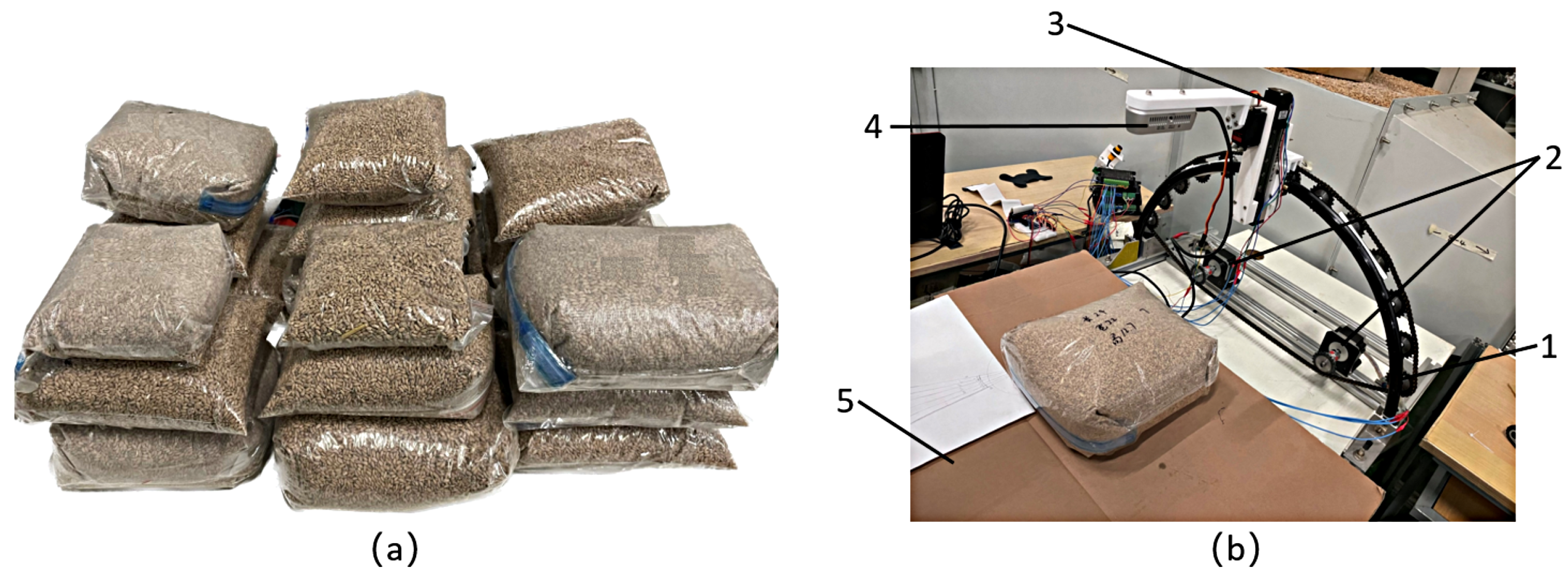
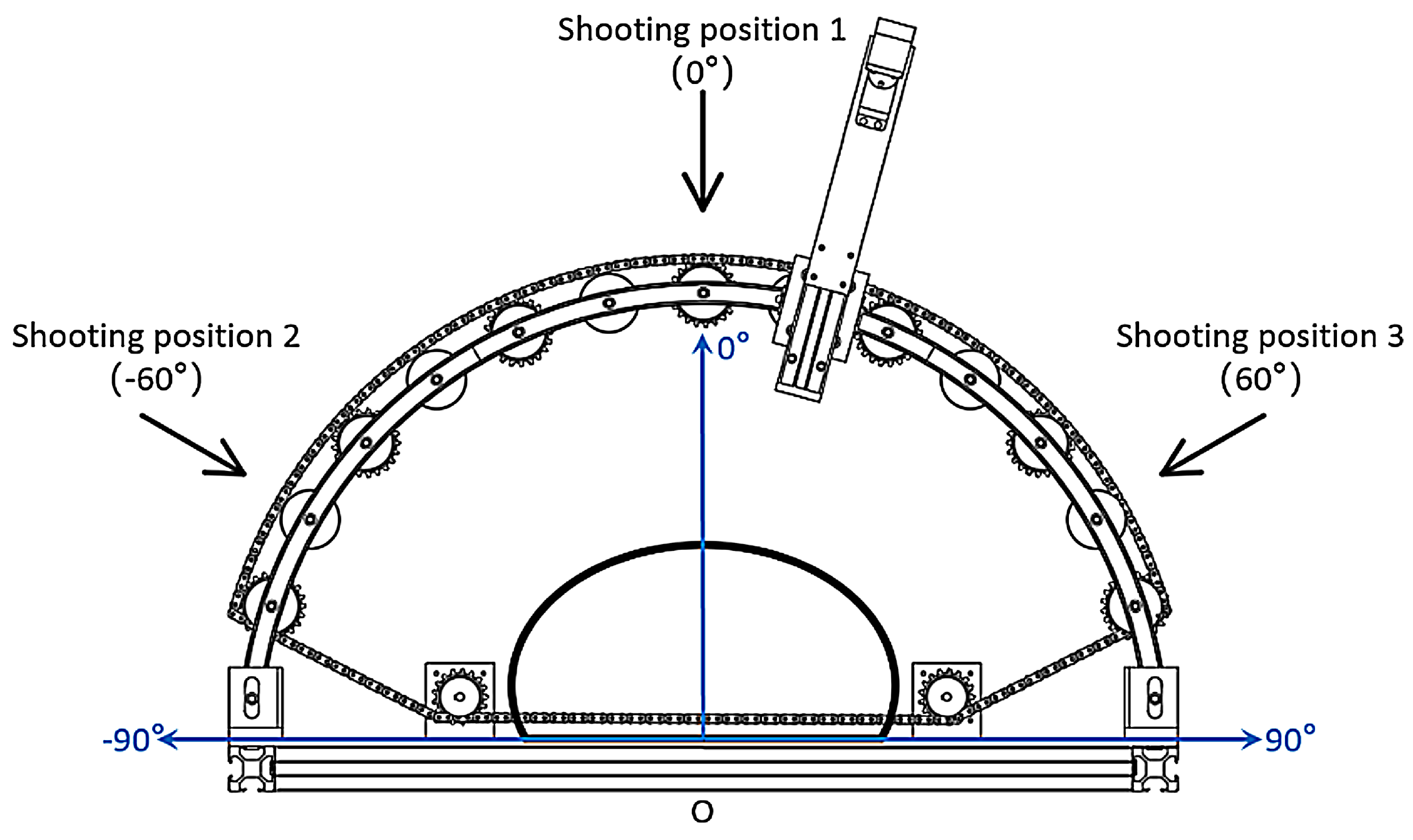
2.1. Image Acquisition System and Dataset Construction

This work prepares 36 bagged-grain samples with different sizes, as shown in Figure 1a, and constructs the dataset using the corresponding multi-angle depth images. Among them, 10 samples are for training Yolo-series models, 5 for determining the best shooting angles, and 21 for testing and validating the reconstruction method and size prediction. During the data acquisition process, the sample is always placed in the middle of the rail and on a plate or a conveyor. Figure 1b shows the proposed image acquisition system, which mainly composes a camera rotating module, shooting-height control module, and camera shooting module.
The camera shooting module incorporates a Raspberry Pi 4B processor and a RealSense D435i depth camera with a 640 × 480 pixel depth image resolution. The images are saved in PNG format. The Raspberry Pi controls all the hardware and modules. Specifically, the camera rotating module employs a motor to move the camera over the circular rail. The shooting-height control module vertically lifts or drops the camera so that we can collect depth images of the sample at different angles and from various heights. Before acquiring images, the acquisition system moves the camera to a certain height. Then, the system starts from the 10° position at the lower right end of the circular rail, collects a depth image every 3°–5°, and stops at 10° on the right. Afterward, the system lifts the camera and repeats the mentioned image acquisition process. In total, this work collects images at 6 heights over 10 samples, resulting in 2394 single-angle depth images.
After collecting all the single-angle depth images, this study produces the rendered images. According to the depth value of each pixel in a depth image, we assign each pixel with the corresponding RGB color value and generate a complete RGB-rendered image. These 2394 rendered images are classified as positive, as shown in Figure 2b. Then, this study prepares another 2394 rendered negative images with the following process. We crop each rendered image so that the grain bags on these images are incomplete. We then enlarge the cropped images to the pixel dimensions of 640 × 480 as those of the positive images. These processed images are marked as negative, as shown in Figure 2c. Consequently, this study obtained a dataset of 4788 images with 50% positive (2394 rendered images) and 50% negative (also 2394 rendered images) images.
LabelImg software is then employed to annotate all the 4788 rendered-depth images. This work annotates the positive or negative of each image. This work then converts all labeled images into visual object class (VOC) format, forming the dataset for Yolo-series neural network models. This study employs 80% of the dataset to train various Yolo-series models and tests the model performance with the remaining 20% of the dataset. This means the training dataset includes 3830 images, and the test dataset has 958 images.

2.2. Bagged-Grain Identification Model Selection

2.2.1. Yolo-Series Neural Networks Training and Model Selection

This paper considers and compares six Yolo-series networks for bagged-grain identification, including Yolo v3, Yolo v5, Yolo v6, YoloX, Yolo v7, and Yolo-Fastest V2. The dataset of 3830 images, incorporating positive and negative rendered-depth images, is utilized for training these models. The main configuration parameters of the computer for training are Intel Core i9-13900K CPU, GeForce RTX 3090 GPU, and 32 GB running memory, and the development environment is Windows 11, PyCharm, CUDA 11.7, and Python 3.9 combined with Torch 2.0.1. For training purposes, we set the initial learning rate of 0.0001, the batch size of 32, the subdivision of 8, and the iteration period of 100. After training each Yolo model, we choose the representative network with the highest recognition accuracy. Then, we test all the selected Yolo models using the test dataset. Since the system requires deploying a neural network model on Raspberry Pi, we compare model size, running speed, and recognition accuracy among all the six selected models to find the optimal one. Therefore, we choose some indicators for testing models, having mean average accuracy (mAP), single frame detection time, and model size.
Table 1 provides the test results. All the other five models, except YoloX, achieve an identification accuracy higher than 99%. The YoloX also achieves a high mAP of 95%. The test verifies that these Yolo-series models can adequately complete the bagged-grain identification task. When considering the single frame detection time and model size, the Yolo-Fastest V2 demonstrates an extraordinary performance, achieving 0.02 s and 0.91 M, respectively. The overall performance of Yolo-Fastest V2 on the bagged-grain identification from the background is more appropriate for the present study than others for spending the least running time and possessing the smallest model size while achieving high accuracy. Therefore, this study selects the Yolo-Fastest V2 for developing the embedded system.

2.2.2. Yolo-Series Neural Networks Training

Figure 3 displays the network structure of the Yolo-Fastest V2 model, whose report studies are still few [26,27,28,29]. Instead of using the original backbone network, the model adopts the ShuffleNet V2 [30] network for the backbone feature extraction, reducing the memory access cost. Such a backbone network also helps enhance the speed and reduce the model weight. As is seen, the model employs the Yolo v5 Anchor matching mechanism to predict the actual detection frame. In addition, Yolo-Fastest V2’s feature map can be decoupled into three different feature maps. Classifying foreground–background and detecting class utilizes the same network branch and shares the parameters, thus achieving a lightweight model.

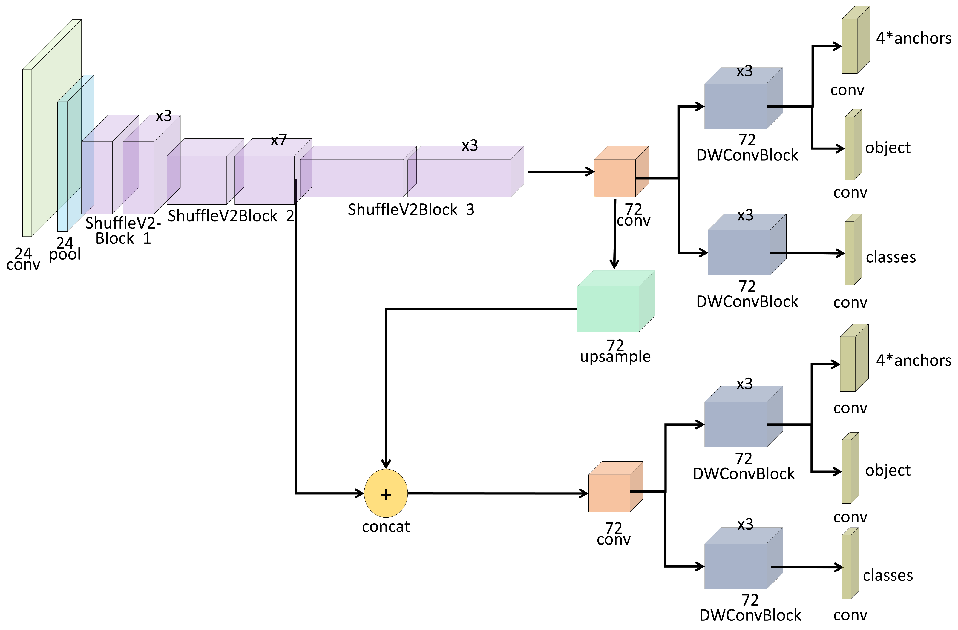
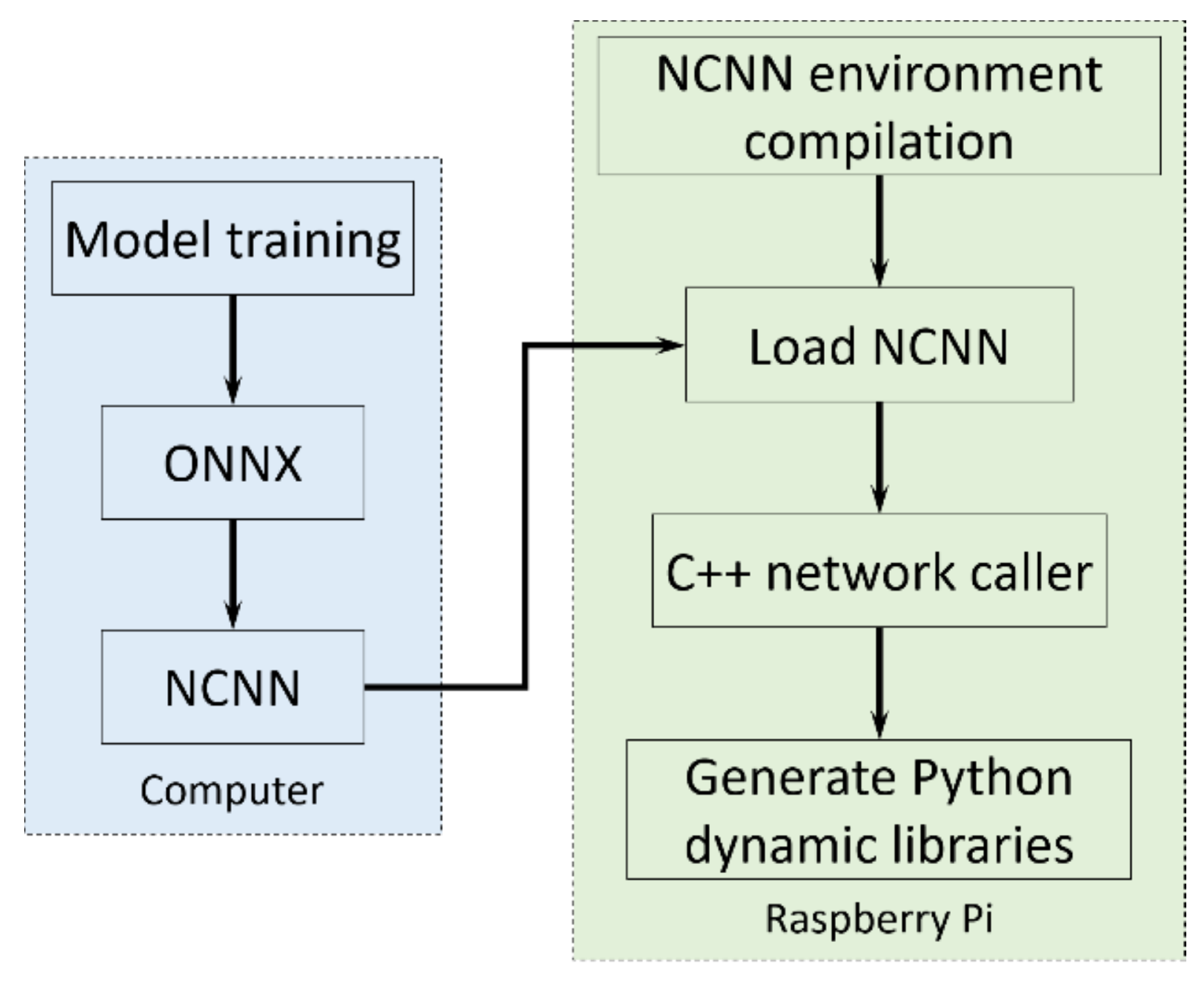
2.2.3. Yolo-Fastest V2 Acceleration on Embedded System

Figure 4 displays the process for accelerating the embedded Yolo-Fastest V2 model. The nano computer neural network (NCNN) is a neural network forward computing framework available for deploying a network on an embedded device [31,32,33]. NCNN initiates its use on mobile phones and achieves, and now it begins to accommodate the Raspberry Pi application. The first step is implemented on a computer, marked by a blue rectangle. This study converts the derived Yolo-Fastest V2 model into the Open Neural Network Exchange ONNX [34] file type and finally converts it to an NCNN model file. Then, this study completes the second step in a Raspberry Pi board, marked by a green rectangle. This study compiles the NCNN environment in a Raspberry Pi and then deploys the NCNN model. Implementing the C++ language for network calls can alleviate the call burden and speed up the embedded system. Finally, this study encapsulates the Python dynamic library using C++ version-based network calling programs.

2.3. Three-Dimensional Reconstruction of Grain Bags

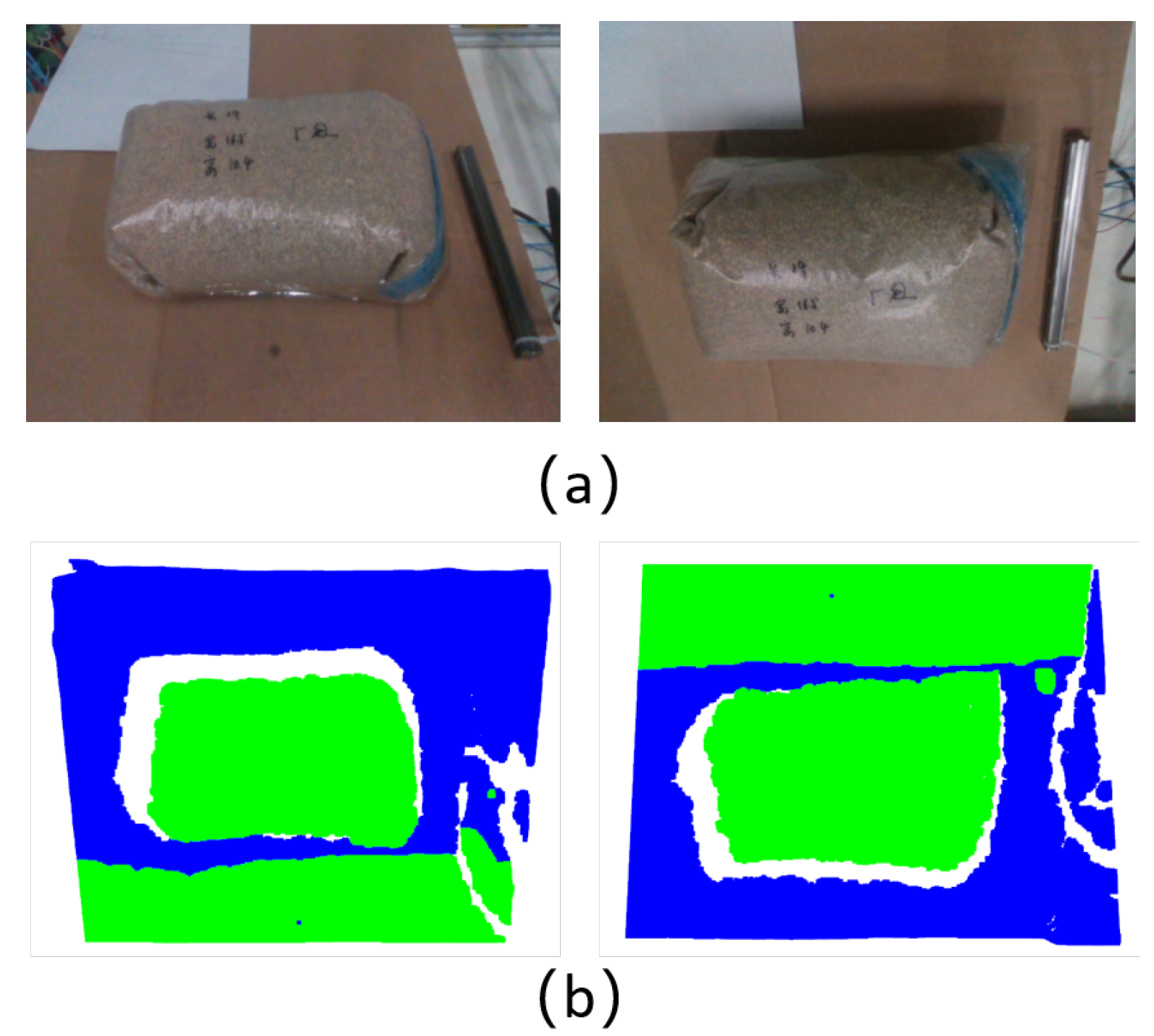
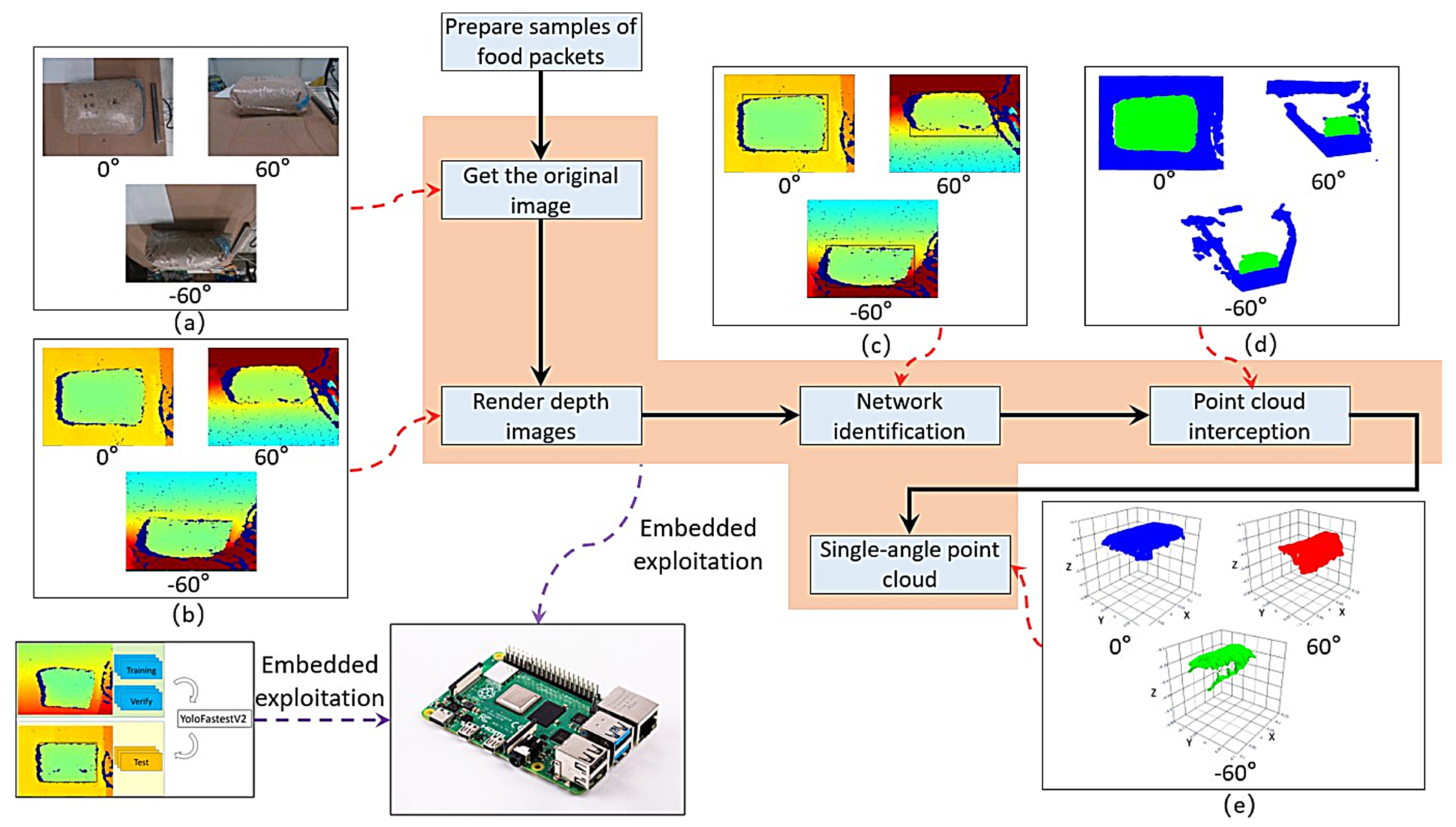
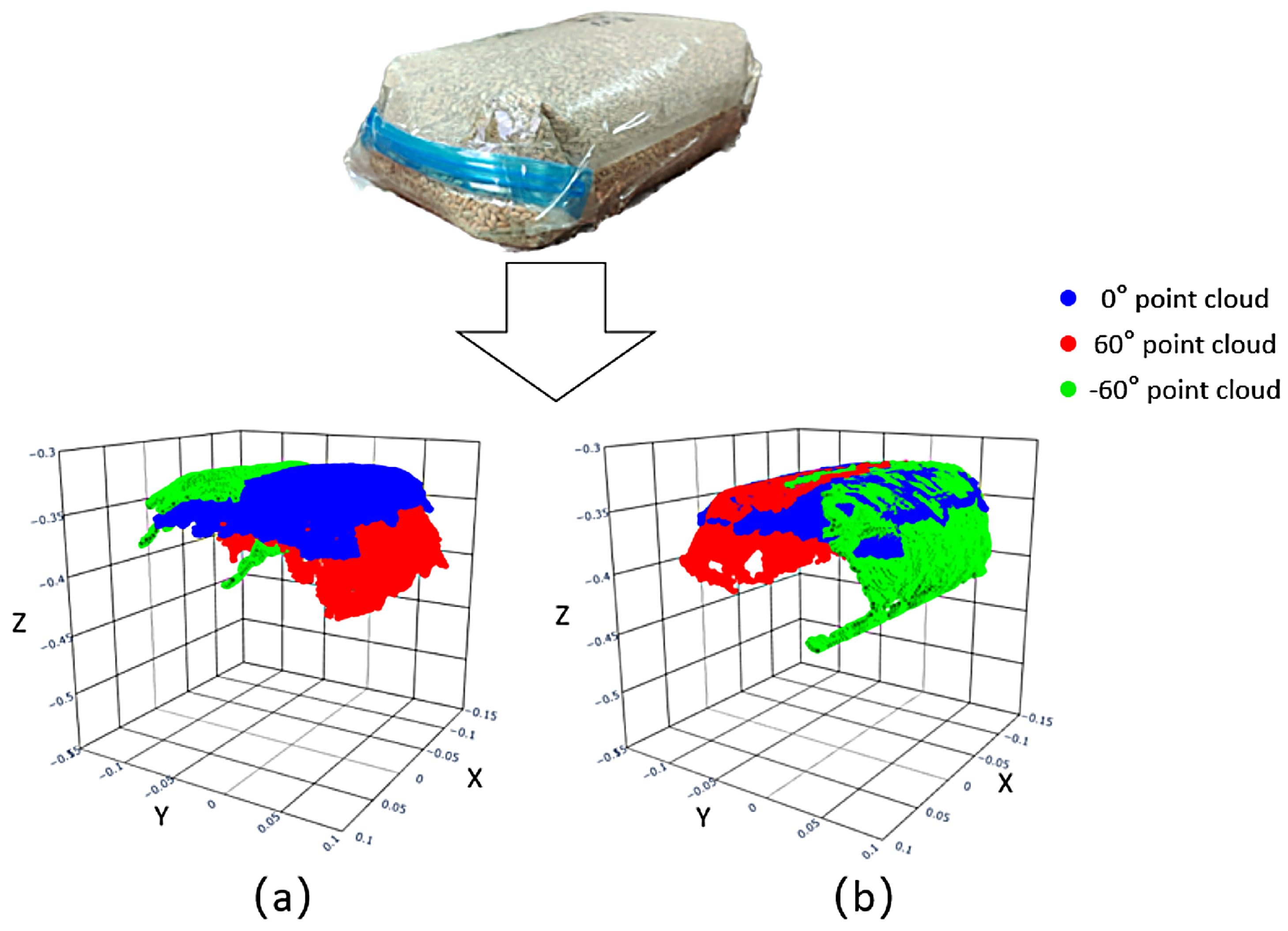
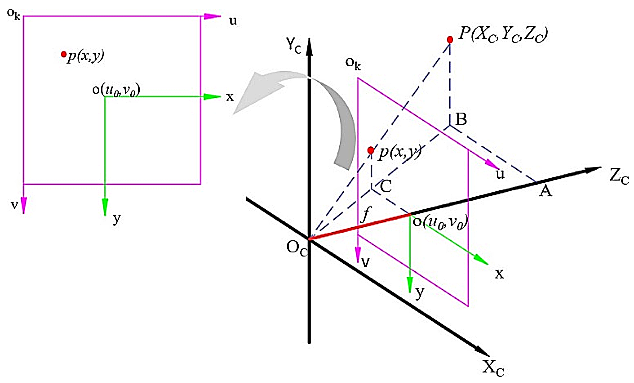
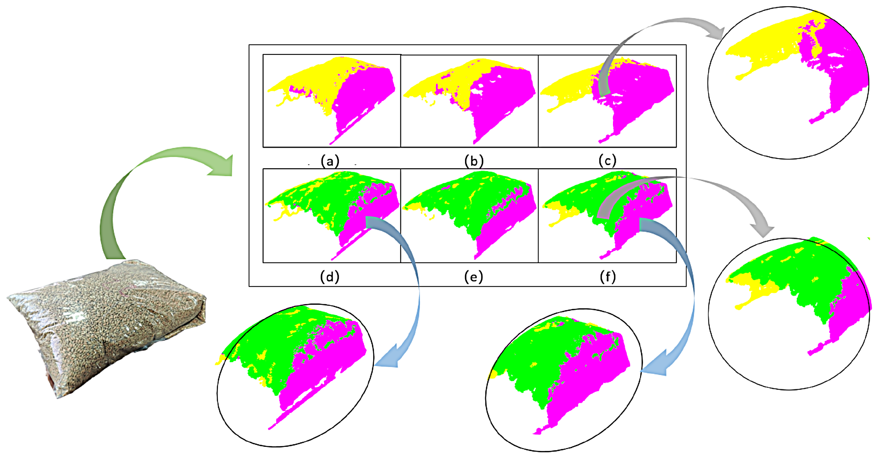
2.3.1. Single-Angle Point-Cloud Extraction Method

Before reconstructing the 3D model for the grain bag, the system is required to collect point-cloud data from different angles. Figure 5 demonstrates the point-cloud acquisition system and the camera shooting of an object at different angles. The angular coordinate’s original 0° is located at the top-head over the grain bag under test. The angle decreases to −90° when the camera rotates to the left and increases to 90° when the camera moves to the right. The collected point clouds are then fused to form a complete point cloud for the object.
When rotating the camera and acquiring a point cloud at a tilt angle, the bag’s surface will have the same depth as the plate plane in the image. Figure 6 demonstrates the point cloud processed by a pass-through filter and denotes a problem in that the green region involves both the bag’s surface and the background. Denoising methods like pass-through filtering are unavailable to remove the background interference and sorely extract the object.
This study develops a novel single-angle point-cloud extraction method using the proposed Yolo-Fastest V2 model to eliminate the background interference and obtain the clear grain bag point clouds. This study provides the transformation between different coordinates shown in Figure 7. Three coordinates are involved, including the pixel, image, and camera coordinates. In the figure, O C X C Y C Z C denotes the camera coordinate, oxy is the image coordinate, and o k uv is the pixel coordinate.
The image and pixel coordinates are two-dimensional, while the camera coordinate is three-dimensional. Any point P ( X C , Y C , Z C ) in the camera coordinate converts to the point p ( x , y ) in the image coordinate via the pinhole camera model. The point p then converts to point in pixel coordinate according to the conversion relationship between the image and pixel coordinates. The conversion from the image coordinate to the pixel coordinate is expression as follows:
u = x d x + u 0 v = y d y + v 0
The matrix form of Equation (1) yields:
u v 1 = 1 d x 0 u 0 0 1 d y v 0 0 0 1 x y 1
where u 0 and v 0 are the location coordinate values of the image coordinate system origin in the pixel coordinate system, x and y are the point p in the 2D image coordinate, and u and v denote the corresponding point in the pixel coordinate.
Using the principle of triangle similarity, we can convert a point in image coordinate to the camera coordinate. Shown by coordinate conversion diagram, the triangle A B O C is similar to the triangle o C O C , and the triangle P B O C is similar to p C O C , which yields A B o C = A O c o O c = P B p C = X C x = Z C f = Y C y . Thus, two coordinates are converted following the equation below:
x = f X C Z C y = f Y C Z C
The matrix form of Equation (3) obtains:
Z C x y 1 = f 0 0 0 0 f 0 0 0 0 1 0 X C Y C Z C 1
where X C , Y C , and Z C represent point P in the 3D camera coordinate, and f is the camera focal length. This study extracts the point cloud of grain bags with the described transformation matrix between coordinates. Figure 8 demonstrates extracting and acquiring the point cloud at each camera shooting angle. The object under test is imaged at different angles, shown in Figure 8a. First, the system employs the Yolo-Fastest V2 model to identify the object in the rendered-depth images (Figure 8b) using a rectangular box, thus obtaining Figure 8c. The system also receives the box’s spatial information in the pixel coordinate and converts it to the corresponding one in the 3D camera coordinate using Equation (2) and Equation (4). Therefore, the 3D object is found and marked by the 3D bounding box. The system intercepts the content within the 3D bounding box and further denoises the content with the pass-through filter, obtaining the final point cloud per each shooting angle (Figure 8d). As a consequence, Figure 8d exhibits the point cloud after Yolo-Fastest V2 model-based identification and interception. Figure 8e presents the extracted single-angle point clouds in the 3D camera coordinate.

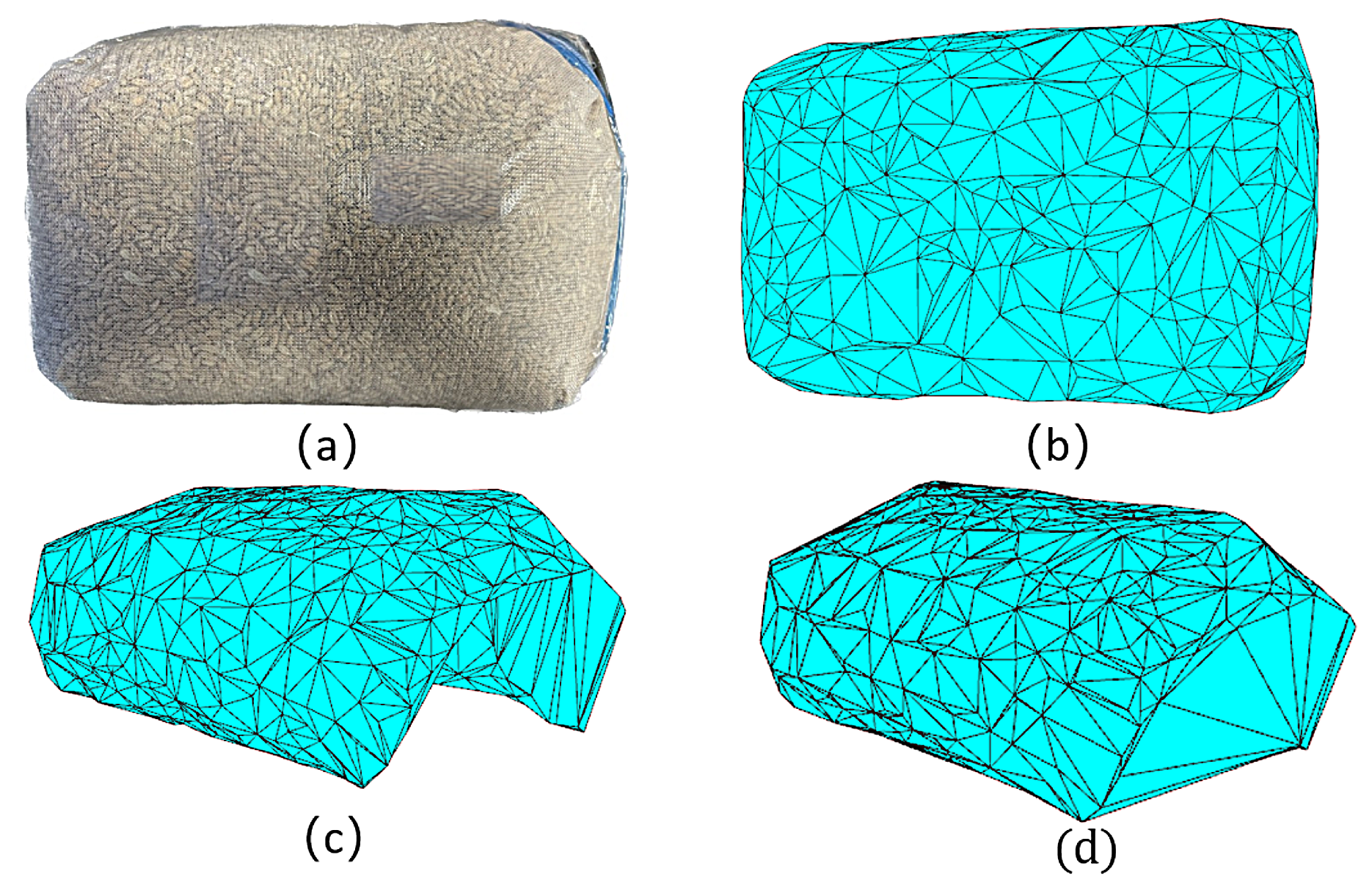
2.3.2. Multi-Angle Point-Cloud Fusion and Surface Reconstruction

After obtaining the single point clouds over the circular rail at different angles, this study investigates the method to properly fuse the point clouds as presented in Figure 9. All the point clouds obtained at different angles are converted to the 3D camera coordinate and are viewed shooting at 0° by default. As a result, the converted point clouds captured at multiple angles overlap and interweave, and the fusion obtains the Figure 9a. Such a problem impedes reconstructing and mapping a correct 3D point-cloud model for the object under test. It is necessary to build a rotation matrix concerning the shooting angle and rotate all the point clouds except the one at 0° to the proper angular position. Since the camera rotates around the X-axis of the camera coordinate, the rotation matrix is written as follows:
p i = 1 0 0 0 cos θ sin θ 0 sin θ cos θ p o
where θ value is the camera shooting angle, and P o and P i represent the original and processed point clouds, respectively. The refined fusion by using the rotation matrix above is presented in Figure 9b. Since the images only cover the optical information of the grain bag’s top surface, the fused 3D model will not reconstruct other characters, such as front, back, and bottom surfaces. So, the fused 3D model has extensive absent areas. Although the Poisson surface [35] reconstruction method is widely used owing to establishing triangles in the low-density region, the fused point cloud is insufficient to reconstruct a complete 3D model of the object by such a method. Thus, this article adopts the α -shape three-dimensional surface reconstruction algorithm [36,37].
The mechanism of the α -shape reconstruction algorithm is to create a polygon shell to simulate the missing regions of an object [38]. The polygon’s vertices are the data on the point cloud. A constant α determines the fineness of the polygon. The smaller the α , the finer the polygon, and the shell is more similar to the actual object. Figure 10 employs the α -shape reconstruction algorithm and tests different α parameters for making up the missing regions and generating a complete bagged-grain 3D model. The figure demonstrates the refined 3D models using two α parameters ( α = 0.1 and α = 0.04). The comparison reveals that only when the α parameter is sufficiently large ( α = 0.1), the refined model is complete with missing or broken parts. Therefore, this study determines α = 0.1 to compensate for the lost regions of the reconstructed 3D model. The system then implements the open3D point-cloud processing library to measure the maximum ( X i m a x , Y i m a x , and Z i m a x ) and minimum ( X i m i n , Y i m i n , and Z i m i n ) values along the X, Y, and Z axes of the i t h reconstructed 3D grain bag model. The system calculates Δ X i the length, Δ Y i the width, and Δ Z i the height for the corresponding object under test. Finally, the system multiplies the Δ X i , Δ Y i , and Δ Z i by a coordinate size conversion coefficient to obtain the target’s actual size. Such a conversion coefficient has been obtained by calibrating the depth camera before its use. Hereto, the size prediction of a bagged grain under test has been completed.

3. Results and Discussion

3.1. Optimal Camera Shooting Layout

Developing an integrated and low-cost monitoring system requires high size prediction accuracy and minimal measurements. This study performs camera shooting tests to determine the optimal shooting angle combination for employing minimal point clouds while achieving high-quality 3D reconstruction. This study prepares 30 angle-combination layouts to reconstruct 5 different grain bags. This study evaluates all the layouts for their performance on reconstruction and size prediction, and Table 2 provides the accuracy per sample and the average accuracy.
The camera shooting test denotes that some two-angle layouts cannot provide a complete 3D reconstruction, and neither can some three angles. As exhibited in Table 2, the reconstructions of (−10°, 10°), (−20°, 20°), (−10°, 0°, 10°), and (−20°, 0°, 20°) reconstruct incomplete bag models and result in a low averaged accuracy due to lacking some lateral information of the target. This study adopts those combinations with an accuracy higher than 97%, which is viewed as accurate. We further investigate the proper and most efficient shooting angle combination among the selected ones to achieve a fast 3D reconstruction. Table 2 also reveals the fact that the average accuracy increases and gradually stabilizes with the presence of additional lateral information. This study chooses six angle combinations, including (−40°, 40°), (−50°, 50°), (−60°, 60°), (−40°, 0°, 40°), (−50°, 0°, 50°), and (−60°, 0°, 60°), for the sake of a minimal shooting layout and the lowest cost. Figure 11 visualizes the results and zooms into the details.
Figure 11 presents the reconstructions of the selected camera shooting combinations and found that two-angle reconstructions lack extensive points on the upper front surface and denote a missing area. The circles zoom the corresponding area in both (−60°, 60°) and (−60°, 0°, 60°) reconstructions. The comparison apparently denotes the vacancy in the (−60°, 60°) one. As is seen, the three-angle reconstruction scheme performs better than the two-angle combinations. This work further compares different three-angle reconstructions and determines the most proper one. In the (−40°, 0°, 40°) and (−60°, 0°, 60°) images, the ellipses zoom the target’s right-bottom area, and the (−40°, 0°, 40°) reconstruction present plenty of blank points. This is because the captured cloud information focuses more on the top-head and less on the alter. When increasing the deflected shooting angle, the reconstruction of the top surface remains the same while the number of blank points is seen to decrease. The (−60°, 0°, 60°) camera shooting layout produces the best result among the proposed three-angle reconstructions. Therefore, this paper selects the angle-combination layout (−60°, 0°, 60°) to reconstruct the grain bag.

3.2. Yolo-Fastest V2 Recognition Speed and Recognition Effect

This study performs tests of 21 grain bags to evaluate the embedded system’s acceleration effect. This work deploys the Torch and NCNN models of the Yolo-Fastest V2 on Raspberry Pi, respectively, and tests the time spent for recognizing 21 groups of samples per shooting angle. According to the previous study, this work adopts the three-angle camera shooting layout (−60°, 0°, 60°). Table 3 provides the recognition time of the two models.
Table 3 shows that the Torch model spends 2660 ms on average for recognizing each point cloud. On the other hand, the NCNN model achieves a much faster recognition task that spends an average recognition time of 82 ms. Figure 12 compares the time spent by each model on recognizing each sample, finding that the NCNN model is nearly 30 times faster than the counterpart. As exhibited, the NCNN greatly accelerates the recognition task on each grain bag sample, thus efficiently accelerating the entire reconstruction process.

3.3. Point Cloud Extraction and 3D Reconstruction Results

This study evaluates the performance of reconstructing 21 bagged-grain samples using the multi-angle point-cloud fusion method proposed in Section 2.3. Table 4 provides each predicted sample size, and Figure 13 compares the predicted value to the measured value. Table 4 demonstrates that the average accuracies of size prediction in length, width, and height are 97.76%, 97.02%, and 96.81%, respectively. Figure 13 compares the size prediction with the actual measurement. In the three plots (a), (b), and (c), the red line in the figure is y = x, and the star denotes the coordinate point composed of the predicted and the measured value. The closer the coordinate point is to y = x, the smaller the error between the predicted and the measured value. The coefficient of determination R 2 and the root mean square error RMSE between the predicted and the measured value are calculated. For length predictions, RMSE is 5.38 mm, and R 2 is 0.9748. The width of RMSE is 5.79 mm, R 2 is 0.9393. For height, the RMSE is 3.45 mm, and the R 2 is 0.9352. All the stars in the three plots are close enough to the straight diagonal line, indicating the normality assumption for the proposed size prediction method. We then calculate the residuals between the prediction and the measured value to quantify their relationship and examine the homoscedasticity of our method. Figure 13d–f show the residual plots between the prediction and fitted value corresponding to each sample’s length, width, and height. In these figures, the straight line exhibits the zero, and the dot denotes the residual. As calculated, all the residuals are close enough to zero, where the maximum residual value of length is 8.53 mm, the one for width is 8.78 mm, and the one for height is 6.94 mm. Moreover, the residuals in the three plots are roughly evenly scattered around zero with no obvious patterns, showing the proposed method is also homoscedasticity. Therefore, our proposed method can appropriately predict the size of grain bags. The main error is dedicated to mechanical construction. Three parts assemble the circular rail, resulting in a non-negligible mechanical construction error. Such a built structure causes the shooting angle deviation and contributes to the primary source of the size prediction error. Moreover, the calibration of the depth camera affects the correctness of the coordinate size conversion, which also contributes to the size prediction error.

4. Conclusions

The present article developed and built an embedded binocular vision system for online measuring in-warehouse grain bag sizes while proposing a novel size prediction method for deep learning and three-dimensional reconstruction. This article verified the proposed method by performing abundant and reasonable tests and concluded as follows:
(1)
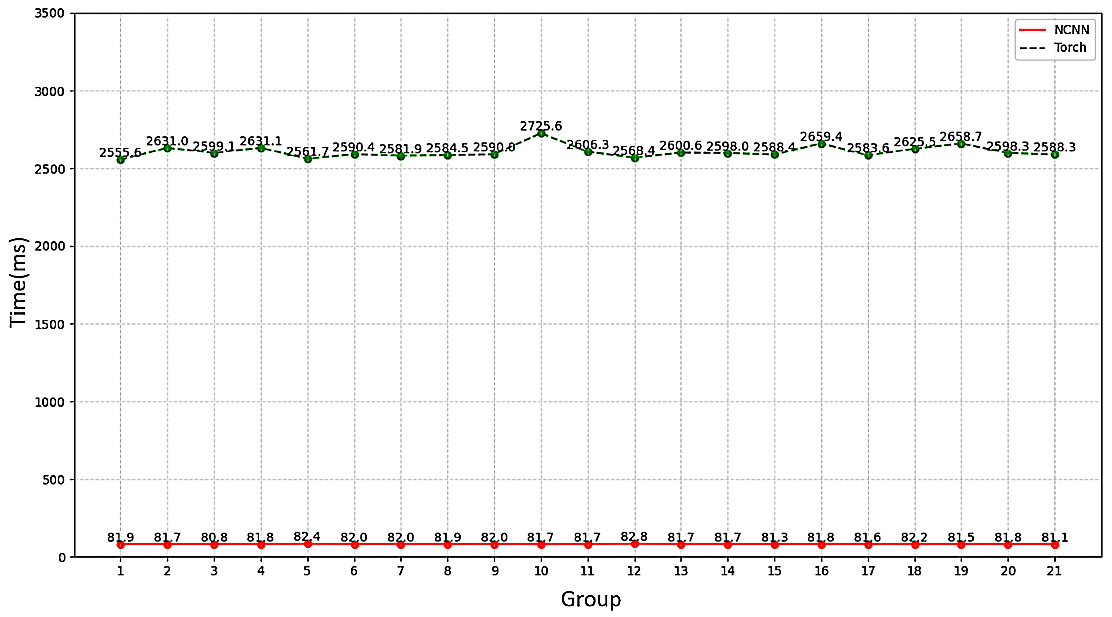
This study trained six Yolo-series neural networks and comprehensively determined the most appropriate one for the system, known as the Yolo-Fastest V2 model. This study deployed the Yolo model on a Raspberry Pi board and introduced the NCNN model to accelerate the embedded system. Tests verified that the NCNN model-based embedded system spent 82 ms on average for processing each single frame image, which was nearly 30 times faster than the original embedded system. From this, this paper developed a novel point-cloud extraction method using the Yolo-Fastest V2 model. This study performed experiments and verified the method’s efficacy in removing interference and obtaining the grain bag point cloud at each shooting angle.
(2)
This work investigated the camera shooting layout by conducting 30 angle-combination layouts to reconstruct five different grain bags and determined the optimal one (−60°, 0°, 60°). Hence, this study constructed the rotation matrix to fuse multi-angle point clouds and merged the α -shape three-dimensional surface reconstruction algorithm into the embedded system to derive a complete 3D model of the target under test. This work further achieved size prediction by obtaining the length, width, and height from the 3D model. The experimental results verified the proposed size prediction method that the averaged accuracies were greater than 96%; moreover, the root mean square error RMSE was less than 7 mm, the maximum residual value was less than 9 mm, and the coefficient of determination R 2 was greater than 0.92.
Overall, the proposed method and embedded Raspberry Pi system met the requirement of online size prediction of in-warehouse bagged and bulk grains and will pave the way for real-time contactless grain moisture monitoring. A more accurate feedback control system will be required to reduce mechanical assembly errors and improve reconstruction accuracy.

Author Contributions

Conceptualization, S.G. and X.M.; methodology, S.G. and D.D.; software, S.G. and D.D.; validation, S.G., X.M. and D.D.; formal analysis, S.G. and X.M.; investigation, S.G. and D.D.; resources, S.G., D.D. and Z.W.; data curation, S.G. and X.M.; writing—original draft preparation, S.G. and X.M.; writing—review and editing, X.M., S.W., D.C. and Z.W.; visualization, D.D. and Z.W.; supervision, X.M. and S.W.; project administration, X.M. and D.C.; funding acquisition, X.M. and Z.W. All authors have read and agreed to the published version of the manuscript.

Funding

This work was supported by the Jiangsu Province Modern Agricultural Equipment and Technology Collaborative Innovation Center Project (XTCX2005), and National Natural Science Foundation Project (32201687).

Data Availability Statement

The data used in this study are available upon request from the corresponding author via email.

Conflicts of Interest

The authors declare no conflict of interest.

References

  1. Promote the saving and loss reduction of grain transportation. China Finance 2022, 1, 28–29.
  2. Song, C. Analysis of Grain Storage Loss Causes and Loss Reduction Measures. Modern Food 2023, 29, 1–3. [Google Scholar]
  3. Han, W. Cause analysis of grain storage loss and countermeasures to reduce consumption and loss. Grain Food Ind. 2022, 29, 61–64. [Google Scholar]
  4. Liu, J.; Qiu, S. Development and application of portable detection device for grain moisture content based on microstrip microwave sensor. J. Food Saf. Qual. Insp. 2022, 13, 5485–5494. [Google Scholar]
  5. Liu, J.; Qiu, S.; Wei, Z. Real-time measurement of moisture content of paddy rice based on microstrip microwave sensor assisted by machine learning strategies. Chemosensors 2022, 10, 376. [Google Scholar] [CrossRef]
  6. Andujar, D.; Ribeiro, A. Using depth cameras to extract structural parameters to assess the growth state and yield of cauliflower crops. Comput. Electron. Agric. 2016, 122, 67–73. [Google Scholar] [CrossRef]
  7. Yin, Y.; Liu, G.; Li, S.; Zheng, Z.; Si, Y.; Wang, Y. A Method for Predicting Canopy Light Distribution in Cherry Trees Based on Fused Point Cloud Data. Remote Sens. 2023, 15, 2516. [Google Scholar] [CrossRef]
  8. Jiang, Y.; Li, C.; Paterson, A. Quantitative analysis of cotton canopy size in field conditions using a consumer-grade RGB-D camera. Front. Plant Sci. 2018, 8, 2233. [Google Scholar] [CrossRef] [PubMed]
  9. Wang, Y.; Chen, Y. Fruit morphological measurement based on three-dimensional reconstruction. Agronomy 2020, 10, 455. [Google Scholar] [CrossRef]
  10. Xie, W.; Wei, S. Morphological measurement for carrot based on three-dimensional reconstruction with a ToF sensor. Postharvest. Biol. Technol. 2023, 197, 112216. [Google Scholar] [CrossRef]
  11. Zhang, L.; Xia, H.; Qiao, Y. Texture Synthesis Repair of RealSense D435i Depth Images with Object-Oriented RGB Image Segmentation. Sensors 2020, 20, 6725. [Google Scholar] [CrossRef] [PubMed]
  12. Jiang, P.; Ergu, D. A Review of Yolo algorithm developments. Procedia Comput. Sci. 2022, 199, 1066–1073. [Google Scholar] [CrossRef]
  13. Kattenborn, T.; Leitloff, J. Review on Convolutional Neural Networks (CNN) in vegetation remote sensing. ISPRS J. Photogramm. Remote Sens. 2021, 173, 24–49. [Google Scholar] [CrossRef]
  14. Lu, W.; Zou, M. Visual Recognition-Measurement-Location Technology for Brown Mushroom Picking Based on YOLO v5-TL. J. Agric. Mach. 2022, 53, 341–348. [Google Scholar]
  15. Jing, L.; Wang, R. Detection and positioning of pedestrians in orchard based on binocular camera and improved YOLOv3 algorithm. J. Agric. Mach. 2020, 51, 34–39+25. [Google Scholar]
  16. Elhassouny, A. Trends in deep convolutional neural Networks architectures: A review. In Proceedings of the 2019 International Conference of Computer Science and Renewable Energies, Agadir, Morocco, 22–24 July 2019; pp. 1–8. [Google Scholar]
  17. Wang, D.; Cao, W.; Zhang, F. A review of deep learning in multiscale agricultural sensing. Remote Sens. 2022, 14, 559. [Google Scholar] [CrossRef]
  18. Gonzalez-Huitron, V.; León-Borges, J. Disease detection in tomato leaves via CNN with lightweight architectures implemented in Raspberry Pi 4. Comput. Electron. Agric. 2021, 181, 105951. [Google Scholar] [CrossRef]
  19. Fan, W.; Hu, J.; Wang, Q. Research on mobile defective egg detection system based on deep learning. J. Agric. Mach. 2023, 54, 411–420. [Google Scholar]
  20. Zeng, T.; Li, S. Lightweight tomato real-time detection method based on improved YOLO and mobile deployment. Comput. Electron. Agric. 2023, 205, 107625. [Google Scholar] [CrossRef]
  21. Zhao, L.; Li, S. Object detection algorithm based on improved YOLOv3. Electronics 2020, 9, 537. [Google Scholar] [CrossRef]
  22. Zhao, J.; Zhang, X. A wheat spike detection method in UAV images based on improved YOLOv5. Remote Sens. 2021, 13, 3095. [Google Scholar] [CrossRef]
  23. Yung, N.; Wong, W. Safety helmet detection using deep learning: Implementation and comparative study using YOLOv5, YOLOv6, and YOLOv7. In Proceedings of the 2022 International Conference on Green Energy, Computing and Sustainable Technology, Miri Sarawak, Malaysia, 26–28 October 2022; pp. 164–170. [Google Scholar]
  24. Ji, W.; Pan, Y. A real-time apple targets detection method for picking robot based on ShufflenetV2-YOLOX. Agriculture 2022, 12, 856. [Google Scholar] [CrossRef]
  25. Wang, C.; Bochkovskiy, A. YOLOv7: Trainable bag-of-freebies sets new state-of-the-art for real-time object detectors. In Proceedings of the IEEE/CVF Conference on Computer Vision and Pattern Recognition, Vancouver, BC, Canada, 18–22 June 2023; pp. 7464–7475. [Google Scholar]
  26. Dog-qiuqiu/Yolo-FastestV2: Based on Yolo’s Low-Power, Ultra-Lightweight Universal Target Detection Algorithm, the Parameter is only 250k, and the Speed of the Smart Phone Mobile Terminal Can Reach 300fps+. Available online: https://github.com/dog-qiuqiu/Yolo-FastestV2github.com (accessed on 3 July 2022).
  27. Zhang, H.; Xu, D.; Cheng, D. An Improved Lightweight Yolo-Fastest V2 for Engineering Vehicle Recognition Fusing Location Enhancement and Adaptive Label Assignment. IEEE J. Sel. Top. Appl. Earth Obs. Remote Sens. 2023, 16, 2450–2461. [Google Scholar] [CrossRef]
  28. Cao, C.; Wan, S.; Peng, G.; He, D.; Zhong, S. Research on the detection method of alignment beacon based on the spatial structure feature of train bogies. In Proceedings of the 2022 China Automation Congress, Chongqing, China, 2–4 December 2022; pp. 4612–4617. [Google Scholar]
  29. Wang, Y.; Bu, H.; Zhang, X. YPD-SLAM: A Real-Time VSLAM System for Handling Dynamic Indoor Environments. Sensors 2022, 22, 8561. [Google Scholar] [CrossRef]
  30. Chen, Z.; Yang, J.; Jiao, H. Garbage classification system based on improved ShuffleNet v2. Resour. Conserv. Recycl. 2022, 178, 106090. [Google Scholar] [CrossRef]
  31. Huang, Y.; Chen, R.; Chen, Y.; Ding, S. A Fast bearing Fault diagnosis method based on lightweight Neural Network RepVGG. In Proceedings of the 4th International Conference on Advanced Information Science and System, Sanya, China, 25–27 November 2022; pp. 1–6. [Google Scholar]
  32. Li, J.; Li, Y.; Zhang, X.; Zhan, R. Application of mobile injection molding pump defect detection system based on deep learning. In Proceedings of the 2022 2nd International Conference on Consumer Electronics and Computer Engineering, Guangzhou, China, 14–16 January 2022; pp. 470–475. [Google Scholar]
  33. Yang, D.; Yang, L. Research and Implementation of Embedded Real-time Target Detection Algorithm Based on Deep Learning. J. Phys. Conf. Ser. 2022, 2216, 012103. [Google Scholar] [CrossRef]
  34. Lin, W.F.; Tsai, D.Y. Onnc: A compilation framework connecting onnx to proprietary deep learning accelerators. In Proceedings of the 2019 IEEE International Conference on Artificial Intelligence Circuits and Systems, Hsinchu, Taiwan, 18–20 March 2019; pp. 214–218. [Google Scholar]
  35. Peng, S.; Jiang, C. Shape as points: A differentiable poisson solver. Adv. Neural Inf. Process. Syst. 2021, 34, 13032–13044. [Google Scholar]
  36. Fu, Y.; Li, C.; Zhu, J. Alpha-shape Algorithm Constructs 3D Model of Jujube Tree Point Cloud. J. Agric. Eng. 2020, 36, 214–221. [Google Scholar]
  37. Huang, X.; Zheng, S.; Zhu, N. High-Throughput Legume Seed Phenotyping Using a Handheld 3D Laser Scanner. Remote Sens. 2022, 14, 431. [Google Scholar] [CrossRef]
  38. Cai, Z.; Jin, C.; Xu, J. Measurement of potato volume with laser triangulation and three-dimensional reconstruction. IEEE Access 2020, 8, 176565–176574. [Google Scholar] [CrossRef]
Figure 1. (a) Thirty-six bagged-grain samples with different sizes. (b) Image acquisition device: 1. circular rail, 2. circular rail motor, 3. shooting-height control module, 4. binocular depth camera, and 5. plate.
Remotesensing 15 04846 g001
Figure 2. Dataset of rendered single-angle depth images. (a) Original RGB images of four grain bag samples, (b) corresponding positive depth images that have complete grain bag samples, and (c) negative depth images that only have a part of the grain bag samples.
Remotesensing 15 04846 g002
Figure 3. Yolo-Fastest V2 model structure. The network structure uses ShuffleNet V2 for the feature extraction and small object prediction, consisting of three Shuffle2Block convolution blocks. Moreover, the structure obtains the feature map by utilizing the convolution of the third convolution block, namely ShuffleV2Block 3. The structure transfers the feature map to the 1 × 1 convolution and yields the upsample. The upsampling features can be fused with the feature map by ShuffleV2Block 2 using a concatenation. The fused feature map is upscaled and can be utilized to predict larger objects.
Remotesensing 15 04846 g003
Figure 4. Flowchart for accelerating Yolo-Fastest V2 embedded model.
Remotesensing 15 04846 g004
Figure 5. Schematic diagram of camera shooting of the grain bag at different angles. The blue line denotes the x–y coordinate of the camera shooting system, with −90° at the left end, 0° in the middle, and 90° at the right end. The system moves the camera over the circular rail and captures original RGB sample images at different shooting angles.
Remotesensing 15 04846 g005
Figure 6. Point clouds captured at different angles and processed by a pass-through filter. (a) Original image of two bagged-grain samples, and (b) corresponding point-cloud images. The green part in (b) represents the plane of multiple objects at the same depth. The point-cloud images denote that the background cannot be effectively removed when the point clouds are processed by pass-through filtering.
Remotesensing 15 04846 g006
Figure 7. Diagram of transformation between different coordinate systems. The figure on the right displays the coordinate transformation from camera coordinate ( O C X C Y C Z C ) to pixel coordinate ( o k uv), where the camera coordinate is three-dimensional, and the pixel coordinate is two-dimensional. Using the proposed matrix, the point P in the three-dimensional coordinate converts to the point p in the two-dimensional coordinate. The figure on the left demonstrates that the pixel and image coordinates are all two-dimensional but have an obvious difference. Equation (1) quantifies such a difference between two coordinates.
Remotesensing 15 04846 g007
Figure 8. Entire process for acquiring the grain bag point cloud at a single angle. (a) The original RGB image, (b) rendered-depth image, (c) recognized image and the bounding box by Yolo-Fastest V2 model, (d) point-cloud interception after pass-through filtering, and (e) extracted single-angle point clouds in the 3D camera coordinate.
Remotesensing 15 04846 g008
Figure 9. Fused point clouds. (a) Original fused point-cloud image, and (b) refined fused point cloud image.
Remotesensing 15 04846 g009
Figure 10. Compensation of the reconstructed 3D models with different α parameters. (a) Top view of the object to be photographed, (b) top view of the 3D reconstruction, (c) lateral view of the 3D reconstruction refinement with α = 0.04, and (d) lateral view of the 3D reconstruction refinement with α = 0.1.
Remotesensing 15 04846 g010
Figure 11. 3D Reconstruction test with six angle combinations, including (a) (−40°, 40°), (b) (−50°, 50°), (c) (−60°, 60°), (d) (−40°, 0°, 40°), (e) (−50°, 0°, 50°), and (f) (−60°, 0°, 60°). Among them, the comparison between (c) and (f), marked by a circle, denotes a better reconstruction of the front end achieved by shooting angles of (−60°, 0°, 60°). The comparison between (d) and (f), marked by an oval, denotes a better reconstruction of the side end achieved by angles of (−60°, 0°, 60°).
Remotesensing 15 04846 g011
Figure 12. Averaged recognition time of the Torch and NCNN models. The green dotted line is for the Torch model recognition time, and the red line exhibits the NCNN model recognition time. In comparison, the recognition speed of the NCNN model is much faster than that of the Torch model.
Remotesensing 15 04846 g012
Figure 13. Comparison between the predicted size and measurement of the bagged-grain sample under test, (a) for the length, (b) for the width, and (c) for the height. The star denotes the intersection between the predicted size and the corresponding measurement of the grain bag, and the red line represents the assumption of y = x. Subfigures (df) indicate the residual values of length, width, and height data for each grain sample, respectively. The middle line denotes the zero.
Remotesensing 15 04846 g013
Table 1. Comparison of Yolo neural network detection results.
InternetmAP 1 (%)Single Frame Detection Time (s)Model Size (M)
Yolo v399.500.3158.65
Yolo v599.650.066.72
Yolo v699.120.064.63
YoloX95.450.168.94
Yolo v799.560.188.71
Yolo-Fastest V299.450.020.91
1 Mean average precision.
Table 2. The average accuracy of reconstruction for camera shooting tests.
Angle CombinationThe Average Accuracy of the Model Size
Reconstruction for Each Grain Package (%)
Average Accuracy
(%)
Group 1 Group 2 Group 3 Group 4 Group 5
(−10°, 10°)80.4582.2382.3985.9883.4382.90
(−20°, 20°)84.2187.3791.9987.4290.4988.30
(−30°, 30°)93.9394.8295.7396.4591.9594.58
(−40°, 40°)95.3197.4598.1197.6596.9797.10
(−50°, 50°)94.5697.4997.3097.6198.4297.08
(−60°, 60°)96.6298.9397.6097.0997.2497.50
(−10°, 0°, 10°)80.9482.4681.2687.7283.4383.16
(−20°, 0°, 20°)84.1487.3793.1588.0490.4988.64
(−30°, 0°, 30°)93.6895.0995.7397.0292.2294.75
(−40°, 0°, 40°)95.2597.9697.1396.8296.8396.80
(−50°, 0°, 50°)96.0297.5097.6997.0598.7097.39
(−60°, 0°, 60°)96.3698.9397.2497.0998.0997.54
(−40°, −10°, 10°, 40°)95.2298.6796.9496.7197.3896.98
(−50°, −10°, 10°, 50°)97.7498.1397.5096.9499.1697.89
(−60°, −10°, 10°, 60°)97.8398.9397.0597.0998.6297.90
(−40°, −20°, 20°, 40°)94.8498.9697.3796.6098.0397.16
(−50°, −20°, 20°, 50°)97.2398.6197.9396.8399.1897.95
(−60°, −20°, 20°, 60°)98.2098.9397.4197.0998.7498.08
(−40°, −30°, 30°, 40°)93.9899.0797.0197.2797.2096.91
(−50°, −30°, 30°, 50°)96.6899.0797.5797.0198.7197.81
(−60°, −30°, 30°, 60°)97.8498.6697.0197.0998.1097.74
(−40°, −10°, 0°, 10°, 40°)95.2298.6797.0596.7197.3897.01
(−50°, −10°, 0°, 10°, 50°)97.7498.1497.3796.9499.1697.87
(−60°, −10°, 0°, 10°, 60°)97.8398.9397.9397.0998.6298.08
(−40°, −20°, 0°, 20°, 40°)94.8498.9697.4196.6098.0397.17
(−50°, −20°, 0°, 20°, 50°)97.2398.6197.0196.8399.1897.77
(−60°, −20°, 0°.20°, 60°)98.2098.9397.5797.0998.7498.11
(−40°, −30°, 0°, 30°, 40°)94.1199.3497.0197.2097.4797.03
(−50°, −30°, 0°, 30°, 50°)96.6899.0797.5797.0198.9897.86
(−60°, −30°, 0°, 30°, 60°)97.7298.6696.9497.0998.3797.75
Table 3. Recognition time of Torch and NCNN models.
PlaceModelRecognition Time (ms)
Group 1Group 2Group 3Group 4Group 5Group 6Group 7
NCNN81.5681.9581.4081.3582.1282.4082.19
Torch2550.132528.782639.192550.342550.492618.772626.05
60°NCNN80.4680.8580.3481.5183.3380.7181.80
Torch2542.582659.312607.072727.882509.182563.882591.62
−60°NCNN83.6082.4280.7882.4081.7782.9381.99
Torch2567.952704.992551.162615.122625.322588.572528.04
Average timeNCNN81.8781.7480.8481.7582.4182.0181.99
Torch2553.552631.022599.142631.112661.662590.412591.90
PlaceModelRecognition Time (ms)
Group 8Group 9Group 10Group 11Group 12Group 13Group 14
NCNN81.8282.6881.8981.8681.7681.2582.40
Torch2551.682618.472701.532529.372537.952532.292671.35
60°NCNN82.4681.7982.6980.7583.9180.7680.98
Torch2623.252589.182759.842694.282598.162591.172526.22
−60°NCNN81.3581.4680.3982.3582.8683.1081.58
Torch2578.592562.292715.372595.192569.142678.232596.31
Average timeNCNN81.8781.9781.6581.6582.8481.7081.65
Torch2584.502589.982725.582606.282568.422600.562597.96
PlaceModelRecognition Time (ms)
Group 15Group 16Group 17Group 18Group 19Group 20Group 21
NCNN80.8281.8281.2882.2581.3880.8981.29
Torch2592.252691.152567.792612.392701.422641.282554.71
60°NCNN80.4780.4180.5781.5981.3681.8680.70
Torch2631.592612.342554.712618.232658.912596.322658.82
−60°NCNN82.5683.1782.8382.6881.8482.5981.18
Torch2541.242674.752628.382645.822615.762557.352551.26
Average timeNCNN81.2881.8081.5682.1781.5381.7881.06
Torch2588.362659.412583.632625.482658.702598.322588.26
Table 4. Prediction of the point-cloud reconstruction size.
GroupLength (mm)Precision
(%)
Width (mm)Precision
(%)
Height (mm)Precision
(%)
Measured
Value
Predicted
Value
ErrorMeasured
Value
Predicted
Value
ErrorMeasured
Value
Predicted
Value
Error
1153151.941.0699.42155158.313.3197.868587.822.8296.68
2225233.068.0696.42190187.932.0798.919094.644.6494.84
3240248.538.5396.45180187.317.3195.949088.431.5798.26
4235243.128.1296.54160167.327.3295.43105107.132.1397.97
5240234.715.2997.80170177.117.1195.82104110.946.9493.33
6205210.435.4397.35175180.125.1297.07118120.322.3298.03
7240235.654.3598.19226232.646.6497.06127130.963.9696.88
8235239.424.4298.11175168.726.2896.41105100.284.7295.51
9283277.325.6897.99225228.833.8398.309896.421.5898.39
10235241.216.2197.36195203.788.7895.508586.911.9197.75
11220226.346.3497.12185189.964.9697.328992.973.9795.54
12210206.333.6798.25185190.625.6296.969593.291.7198.2
13174170.613.3998.05167163.793.2198.077875.462.5496.74
14165169.454.4597.30150155.325.3296.458385.382.3897.13
15186183.782.2298.81177171.585.4296.94109102.696.3194.21
16250256.216.2196.75212215.463.4698.1110299.892.1197.93
17248244.563.4498.61192196.344.3497.74121117.363.6496.99
18251255.564.5698.18215209.475.5397.079496.732.7397.09
19256251.124.8898.09197190.146.8696.528688.062.0697.60
20263267.454.4598.31230221.768.2496.428184.383.3895.83
21272277.715.7197.90220225.475.4797.51112106.842.1698.07
Average
accuracy
97.76 97.02 96.81
Disclaimer/Publisher’s Note: The statements, opinions and data contained in all publications are solely those of the individual author(s) and contributor(s) and not of MDPI and/or the editor(s). MDPI and/or the editor(s) disclaim responsibility for any injury to people or property resulting from any ideas, methods, instructions or products referred to in the content.

