


Soil Salinity Estimation for South Kazakhstan Based on SAR Sentinel-1 and Landsat-8,9 OLI Data with Machine Learning Models
 ,
,  ,
,  ,
,  ,
,  , and
, and
Abstract
:1. Introduction
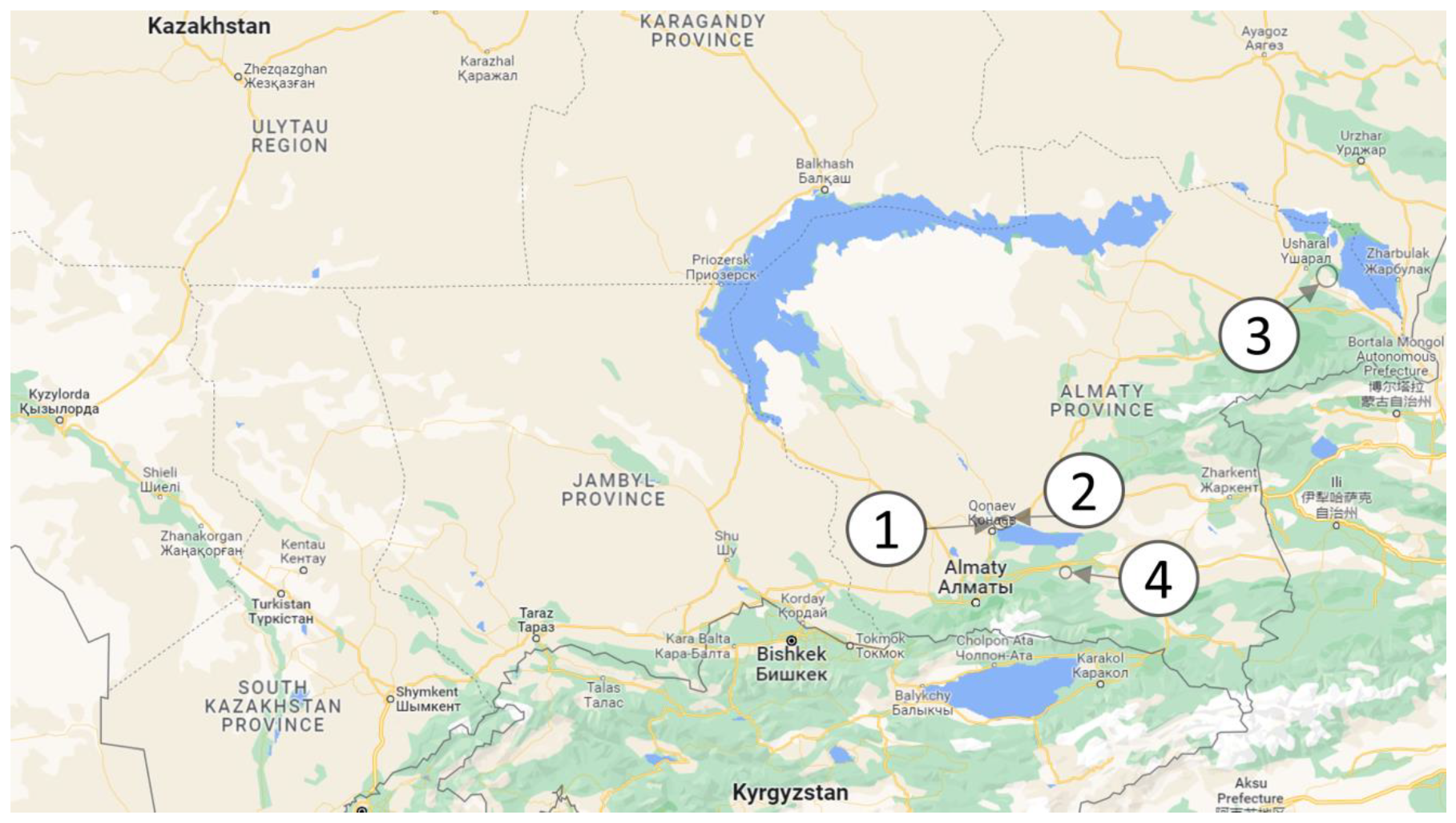
- A set of field data for the study of salinity in the southern regions of Kazakhstan was prepared;
- The method of soil salinity assessment based on SAR data proposed earlier in the literature was supplemented;
- The method of salinity assessment was extended by using a combination of multispectral and SAR radar data;
- A comparative analysis of machine learning algorithms solving the salinity estimation problem on the proposed data set is performed;
- The significant input parameters (features) were selected and their effect was estimated using the methods of explainable machine learning (EML);
- The boundaries of the joint use of obtained field data were determined;
- The obtained modeling results were compared with the results of one of the known models of soil salinity assessment.
2. Related Works
2.1. Classical Salinity Estimation Methods Based on Spectral Data
2.2. Machine Learning Methods in Salinity Estimation Problems
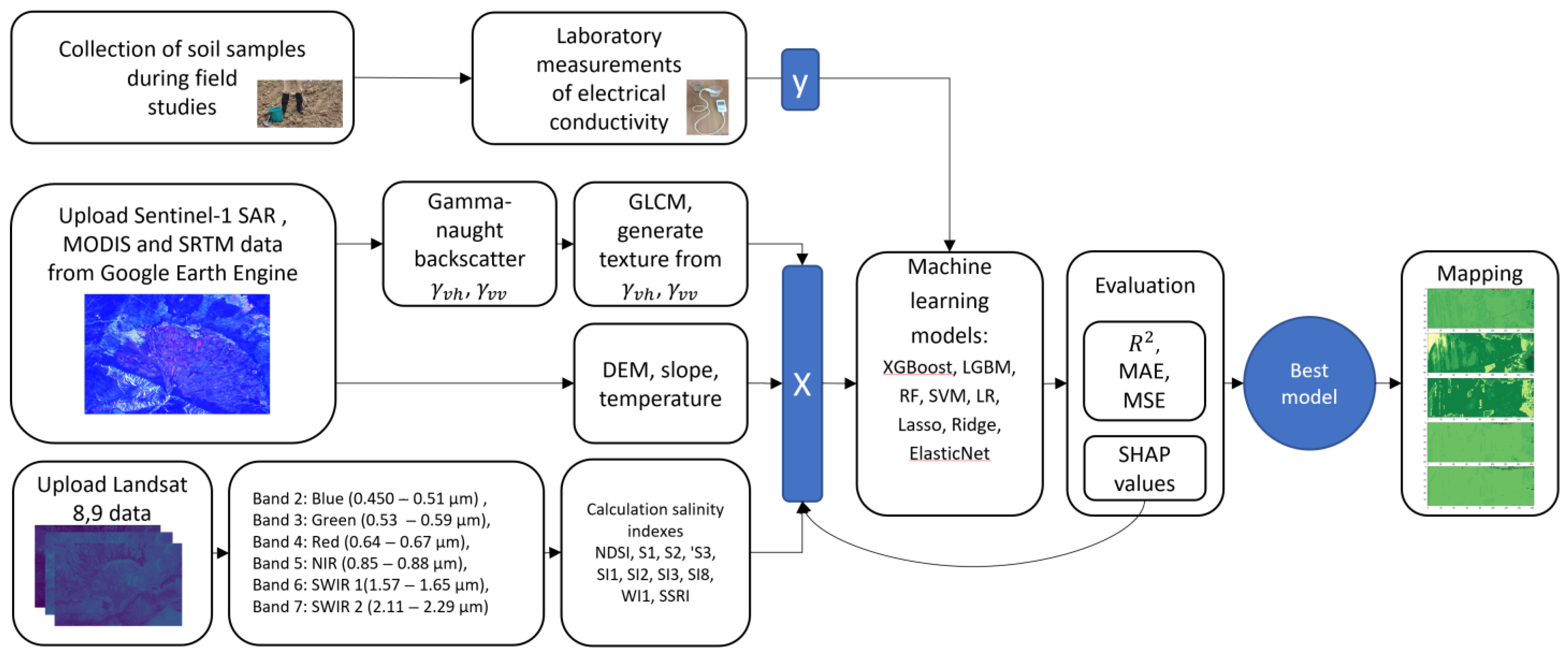
3. Method
- Obtaining the salinity data using the field studies;
- Obtaining the radar, multispectral and SRTM data from Google Earth Engine;
- Extraction of linear back scattering intensity in VV and VH polarizations;
- Texture analysis using the GLCM method;
- Application of the machine learning algorithms and evaluation of the quality of the trained model;
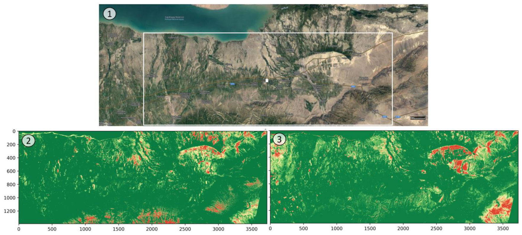
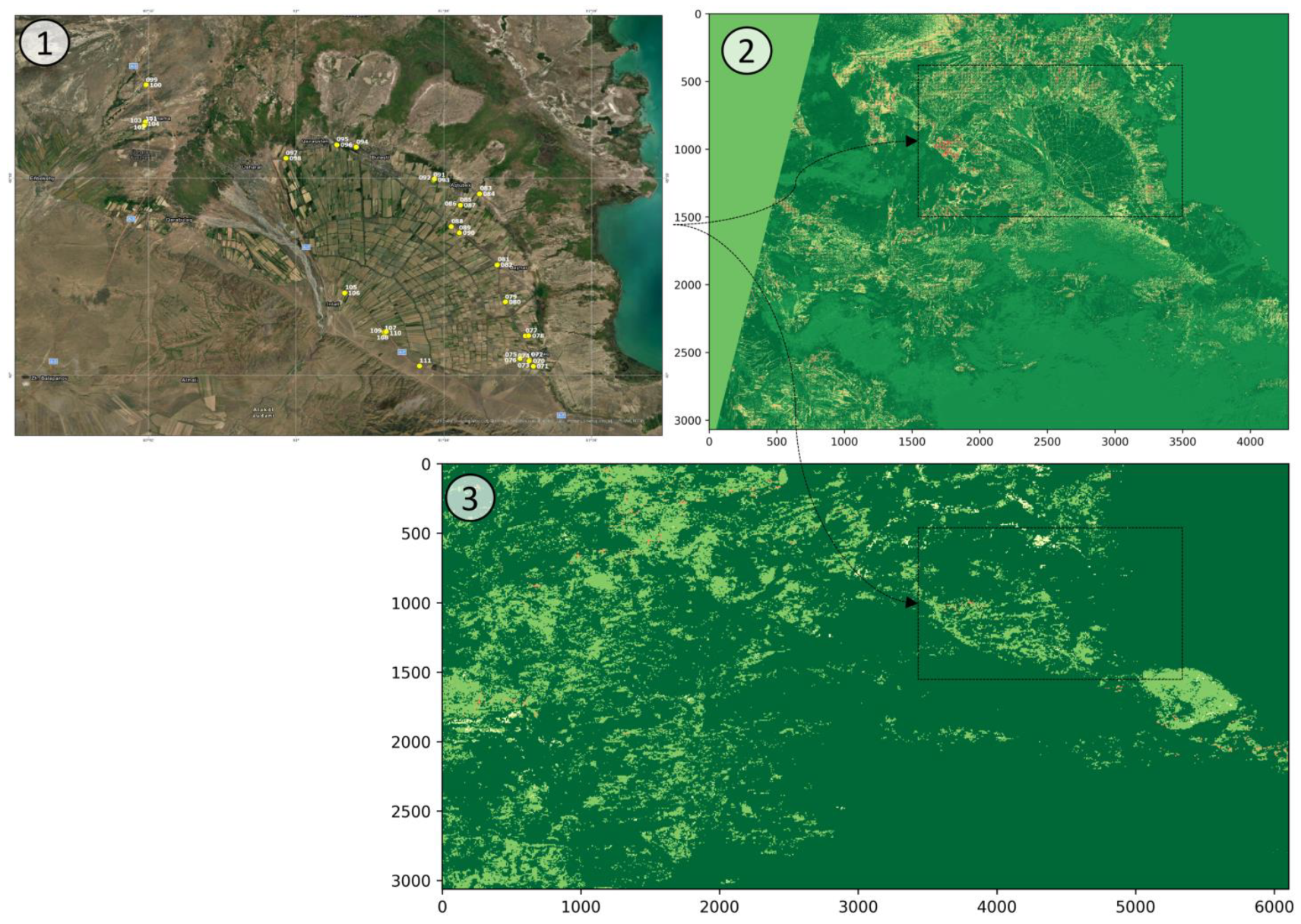
- Mapping the selected areas of the territory.
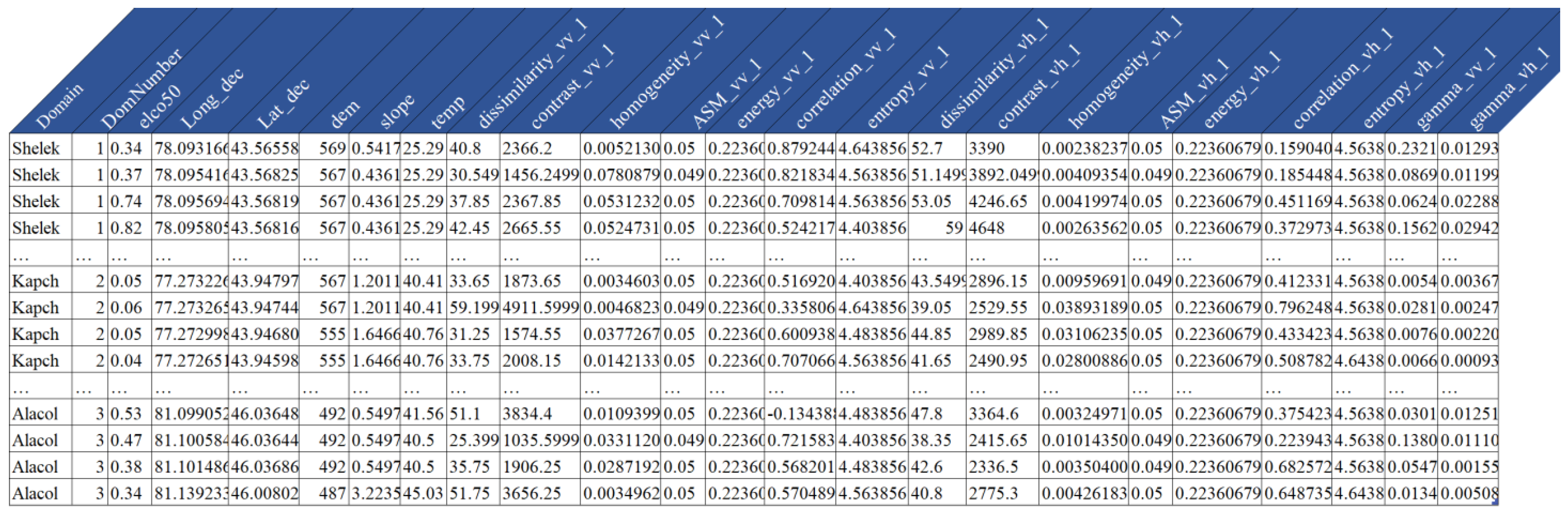
3.1. Data Preparation
3.2. Analysis of Data
3.3. Machine Learning Models
4. Results
4.1. Evaluation of Regression Models
4.2. Analysis of Influence of Input Parameters
5. Discussion
- XGBRegressor has the best quality indicators for the considered regressors; LightGBM is the second in terms of quality indicators.
- The results of the constructed regression are significantly better on moist cultivated soil (Shelek) than on the entire data set.
- The quality of work on the datasets from Alakol and Kapchagay is low. It can be assumed that sampling in a local area of hilly terrain (Kapchagay) and large sampling areas in the Alakol region require a more laborious process of soil data generation, for example, in the form of five-spot sampling [38].
- Comparison of the results of the XGB regressor with the Mtemp model shows that the models produce significantly different results. It can be assumed that a possible reason for the discrepancy is that Mtemp was trained without using data from the regions of Kazakhstan.
6. Conclusions
- A labeled data set is proposed for the electrical conductivity of soils in Southern Kazakhstan, which differ significantly in their geographical location;
- The method of soil salinity estimation described in [33] has been modified and extended with optical data;
- An analysis of several types of machine learning models was performed and it was shown that boosting regression models generally gives the best result;
- The results of the developed model are compared with the results of the Mtemp model [44] and it is shown that the developed model provides better agreement with ground-based measurements of electrical conductivity for this region.
- This study is based on a relatively small amount of field data, which differ significantly in geophysical indicators of collection sites and collection times;
- The quality of the work on the regressors significantly depends on the settings. Despite the search for the best combinations of parameters, it is not possible to analyze all combinations in a limited study;
- The considered set of input parameters is not exhaustive. It is quite acceptable to use the remote sensing data both close to the time of sampling and remote in time.
- Evaluate the effect on the data of optical range, including infrared, on regression quality, depending on the time of remote sensing data acquisition;
- Evaluate the impact of optical and radar data collected within the vegetation growth season (April–August) or for a longer period of time;
- Apply deep learning models to account for terrain parameters;
- Evaluate the possibilities of using multispectral images acquired from a UAV for mapping of focal salinity of agricultural fields.
Supplementary Materials
Author Contributions
Funding
Data Availability Statement
Conflicts of Interest
Abbreviations
| AI | Artificial intelligence |
| BC | Backscattering coefficient |
| BEX | Base exchange index |
| CARS | Competitive adaptive sampling with re-weighting |
| DEM | Digital elevation models |
| DSM | Digital surface model |
| EC | Electrical conductivity |
| ELV | Ground elevation model |
| EML | Explainable machine learning |
| FFNN | Feed-forward neural networks |
| GA | Genetic algorithm |
| GIS | Geographical information system |
| GLCM | Gray level co-occurrence matrix |
| GPS | Global positioning system |
| GQISWI | Groundwater quality index for seawater intrusion |
| LST | Land surface temperature |
| MAE | Mean absolute error |
| ML | Machine learning |
| MSE | Mean squared error |
| NDSI | Normalized differential salinity index |
| R2 | Coefficient of determination |
| RF | Random forest |
| RMSE | Root mean square error |
| SAR | Synthetic Aperture Radar |
| SHAP | SHapley Additive exPlanations |
| SRTM | Shuttle radar topography mission |
| SVM | Support vector machine |
| SWI | Seawater intrusion |
| UAVs | Unmanned aerial vehicles |
| varMAE | variance of MAE |
| varMSE | variance of MSE |
| VarR2 | variance of R2 |
| VIP | variable in projection |
Appendix A. Results of Machine Learning Models Using SAR Data
| Dataset | Regressor | MAE | MSE | VarMAE | VarMSE | Duration | ||
| Alakol | XGB | 0.259 | 0.345 | −1.166 | 0.027 | 0.354 | 2.621 | 15.78875 |
| RF | 0.291 | 0.437 | −6.881 | 0.026 | 0.307 | 135.626 | 18.61323 | |
| LR | 0.646 | 1.139 | −39.321 | 0.048 | 0.857 | 3832.852 | 0.302191 | |
| Lasso | 0.257 | 0.386 | −1.103 | 0.025 | 0.466 | 2.082 | 0.297237 | |
| ElasticNet | 0.257 | 0.386 | −1.103 | 0.025 | 0.466 | 2.082 | 0.294212 | |
| LGBM | 0.257 | 0.386 | −1.103 | 0.025 | 0.466 | 2.082 | 14.26181 | |
| Ridge | 0.322 | 0.468 | −4.645 | 0.022 | 0.479 | 31.485 | 0.595438 | |
| SVM | 0.26 | 0.407 | −1.787 | 0.028 | 0.466 | 12.747 | 0.342054 | |
| Kapchagay | XGB | 0.695 | 3.47 | −0.267 | 0.146 | 19.541 | 0.967 | 7.313395 |
| RF | 1.132 | 5.466 | −11.663 | 0.139 | 18.937 | 664.386 | 21.02584 | |
| LR | 1.412 | 5.04 | −10.429 | 0.085 | 14.996 | 517.132 | 0.341087 | |
| Lasso | 0.821 | 3.57 | −1.212 | 0.099 | 19.35 | 11.81 | 0.328122 | |
| ElasticNet | 0.821 | 3.57 | −1.212 | 0.099 | 19.35 | 11.81 | 0.31415 | |
| LGBM | 0.772 | 3.501 | −1.058 | 0.103 | 19.255 | 11.672 | 18.87905 | |
| Ridge | 0.905 | 3.798 | −2.641 | 0.09 | 18.475 | 37.292 | 0.699129 | |
| SVM | 0.683 | 3.541 | −0.34 | 0.138 | 20.373 | 1.377 | 0.373001 | |
| Shelek | XGB | 0.665 | 0.864 | 0.473 | 0.032 | 0.209 | 0.038 | 50.68989 |
| RF | 0.673 | 0.893 | 0.432 | 0.028 | 0.187 | 0.074 | 21.53441 | |
| LR | 0.813 | 1.25 | 0.186 | 0.037 | 0.567 | 0.245 | 0.352057 | |
| Lasso | 1.1 | 1.778 | −0.104 | 0.028 | 0.374 | 0.02 | 0.330147 | |
| ElasticNet | 1.1 | 1.778 | −0.104 | 0.028 | 0.374 | 0.02 | 0.311206 | |
| LGBM | 0.733 | 0.975 | 0.387 | 0.026 | 0.154 | 0.034 | 24.82316 | |
| Ridge | 0.821 | 1.016 | 0.349 | 0.019 | 0.125 | 0.038 | 0.698132 | |
| SVM | 0.888 | 1.243 | 0.233 | 0.031 | 0.296 | 0.04 | 0.386967 | |
| Full Dataset | XGB | 0.644 | 1.991 | 0.282 | 0.024 | 3.542 | 0.046 | 28.14647 |
| RF | 0.738 | 2.318 | 0.093 | 0.026 | 3.956 | 0.131 | 28.71924 | |
| LR | 0.913 | 2.515 | −0.02 | 0.027 | 3.805 | 0.033 | 0.406411 | |
| Lasso | 0.991 | 2.522 | −0.043 | 0.023 | 3.372 | 0.005 | 0.380981 | |
| ElasticNet | 0.991 | 2.522 | −0.043 | 0.023 | 3.372 | 0.005 | 0.355016 | |
| LGBM | 0.814 | 2.178 | 0.183 | 0.033 | 3.721 | 0.029 | 11.27983 | |
| Ridge | 0.884 | 2.421 | 0.044 | 0.023 | 3.849 | 0.023 | 1.218743 | |
| SVM | 0.791 | 2.27 | 0.139 | 0.031 | 3.681 | 0.018 | 0.627324 |
Appendix B. Results of Machine Learning Models Using SAR Data and Spectral Indices
| Dataset | Regressor | MAE | MSE | VarMAE | VarMSE | Duration | ||
| Alakol | XGB | 0.262 | 0.393 | −0.713 | 0.035 | 0.419 | 2.186 | 22.36715 |
| RF | 0.324 | 0.512 | −7.397 | 0.034 | 0.392 | 201.885 | 19.18279 | |
| LR | 2.862 | 39.064 | −1615.6 | 6.169 | 20,898.03 | 19,891,723 | 0.36007 | |
| Lasso | 0.289 | 0.47 | −1.323 | 0.033 | 0.619 | 3.127 | 0.32513 | |
| ElasticNet | 0.289 | 0.47 | −1.323 | 0.033 | 0.619 | 3.127 | 0.30421 | |
| LGBM | 0.289 | 0.47 | −1.323 | 0.033 | 0.619 | 3.127 | 7.095027 | |
| Ridge | 0.379 | 0.56 | −6.025 | 0.032 | 0.539 | 63.356 | 1.782234 | |
| SVM | 0.291 | 0.468 | −1.398 | 0.032 | 0.608 | 3.588 | 0.345077 | |
| Kapchagay | XGB | 0.66 | 3.153 | −0.342 | 0.135 | 18.206 | 1.532 | 10.36428 |
| RF | 0.9 | 4.667 | −7.927 | 0.147 | 19.196 | 572.823 | 25.85497 | |
| LR | – | – | – | – | – | – | – | |
| Lasso | 0.821 | 3.57 | −1.212 | 0.099 | 19.35 | 11.81 | 0.321146 | |
| ElasticNet | 0.821 | 3.57 | −1.212 | 0.099 | 19.35 | 11.81 | 0.310198 | |
| LGBM | 0.757 | 3.335 | −0.779 | 0.12 | 17.878 | 6.863 | 8.376564 | |
| Ridge | 0.919 | 4.044 | −3.189 | 0.102 | 19.936 | 57.022 | 2.297855 | |
| SVM | 0.675 | 3.518 | −0.286 | 0.137 | 20.212 | 1.221 | 0.424862 | |
| Shelek | XGB | 0.508 | 0.579 | 0.654 | 0.02 | 0.101 | 0.018 | 46.30717 |
| RF | 0.576 | 0.75 | 0.527 | 0.03 | 0.161 | 0.065 | 23.09414 | |
| LR | – | – | – | – | – | – | – | |
| Lasso | 1.1 | 1.778 | −0.104 | 0.028 | 0.374 | 0.02 | 0.336103 | |
| ElasticNet | 1.1 | 1.778 | −0.104 | 0.028 | 0.374 | 0.02 | 0.30322 | |
| LGBM | 0.655 | 0.793 | 0.508 | 0.024 | 0.115 | 0.024 | 9.146147 | |
| Ridge | 0.74 | 0.94 | 0.395 | 0.031 | 0.183 | 0.088 | 1.973743 | |
| SVM | 0.971 | 1.473 | 0.1 | 0.03 | 0.388 | 0.028 | 0.391953 | |
| Full Dataset | XGB | 0.569 | 1.889 | 0.339 | 0.023 | 3.49 | 0.057 | 28.16568 |
| RF | 0.692 | 2.349 | 0.058 | 0.032 | 3.925 | 0.276 | 39.8665 | |
| LR | 0.923 | 2.43 | −0.095 | 0.023 | 2.712 | 0.184 | 0.409904 | |
| Lasso | 0.991 | 2.522 | −0.043 | 0.023 | 3.372 | 0.005 | 0.375001 | |
| ElasticNet | 0.991 | 2.522 | −0.043 | 0.023 | 3.372 | 0.005 | 0.338127 | |
| LGBM | 0.69 | 1.935 | 0.325 | 0.03 | 3.707 | 0.048 | 11.27485 | |
| Ridge | 0.795 | 2.211 | 0.145 | 0.02 | 3.66 | 0.055 | 4.66742 | |
| SVM | 0.811 | 2.242 | 0.145 | 0.029 | 3.573 | 0.015 | 0.791433 |
Appendix C. Regressor Results Using an Optimized Set of Spectral Indices
| Full Dataset | XGB | 0.587 | 1.93 | 0.305 | 0.027 | 3.455 | 0.048 | 23.44931 |
| RF | 0.706 | 2.485 | −0.064 | 0.032 | 3.792 | 0.486 | 27.9018 | |
| LR | 0.8 | 2.147 | 0.136 | 0.021 | 3.152 | 0.057 | 0.404916 | |
| Lasso | 0.991 | 2.522 | −0.043 | 0.023 | 3.372 | 0.005 | 0.378987 | |
| ElasticNet | 0.991 | 2.522 | −0.043 | 0.023 | 3.372 | 0.005 | 0.352054 | |
| LGBM | 0.646 | 1.939 | 0.321 | 0.023 | 3.733 | 0.046 | 10.58872 | |
| Ridge | 0.732 | 2.043 | 0.266 | 0.02 | 3.742 | 0.037 | 1.028286 | |
| SVM | 0.556 | 1.958 | 0.336 | 0.032 | 3.936 | 0.059 | 0.628671 |
Appendix D. Results of Regressors with Optimized SAR Dataset and Optical Indices
| Full Dataset | XGB | 0.575 | 1.858 | 0.356 | 0.023 | 3.526 | 0.061 | 36.6489 |
| RF | 0.685 | 2.275 | 0.109 | 0.027 | 3.875 | 0.176 | 23.21074 | |
| LR | 0.88 | 2.412 | −0.065 | 0.021 | 3.024 | 0.225 | 0.240527 | |
| Lasso | 0.991 | 2.522 | −0.043 | 0.023 | 3.372 | 0.005 | 0.152631 | |
| ElasticNet | 0.991 | 2.522 | −0.043 | 0.023 | 3.372 | 0.005 | 0.155417 | |
| LGBM | 0.671 | 1.971 | 0.314 | 0.023 | 3.89 | 0.051 | 3.863818 | |
| Ridge | 0.764 | 2.104 | 0.221 | 0.02 | 3.671 | 0.033 | 1.490418 | |
| SVM | 0.71 | 2.053 | 0.273 | 0.029 | 3.786 | 0.034 | 0.38091 |
References
- Li, X.; Wang, Z.; Song, K.; Zhang, B.; Liu, D.; Guo, Z. Assessment for salinized wasteland expansion and land use change using GIS and remote sensing in the west part of Northeast China. Environ. Monit. Assess. 2007, 131, 421–437. [Google Scholar]
- Metternicht, G.I.; Zinck, J. Remote sensing of soil salinity: Potentials and constraints. Remote Sens. Environ. 2003, 85, 1–20. [Google Scholar]
- Muhetaer, N.; Nurmemet, I.; Abulaiti, A.; Xiao, S.; Zhao, J. An Efficient Approach for Inverting the Soil Salinity in Keriya Oasis, Northwestern China, Based on the Optical-Radar Feature-Space Model. Sensors 2022, 22, 7226. [Google Scholar] [CrossRef]
- Taghadosi, M.M.; Hasanlou, M.; Eftekhari, K. Soil salinity mapping using dual-polarized SAR Sentinel-1 imagery. Int. J. Remote Sens. 2019, 40, 237–252. [Google Scholar] [CrossRef]
- Grissa, M.; Abdelfattah, R.; Mercier, G.; Zribi, M.; Chahbi, A.; Lili-Chabaane, Z. Empirical model for soil salinity mapping from SAR data. In Proceedings of the 2011 IEEE International Geoscience and Remote Sensing Symposium, Vancouver, BC, Canada, 24–29 July 2011; pp. 1099–1102. [Google Scholar]
- Tripathi, A.; Tiwari, R.K. A simplified subsurface soil salinity estimation using synergy of SENTINEL-1 SAR and SENTINEL-2 multispectral satellite data, for early stages of wheat crop growth in Rupnagar, Punjab, India. Land Degrad. Dev. 2021, 32, 3905–3919. [Google Scholar] [CrossRef]
- Mohamed, S.A.; Metwaly, M.M.; Metwalli, M.R.; AbdelRahman, M.A.; Badreldin, N. Integrating Active and Passive Remote Sensing Data for Mapping Soil Salinity Using Machine Learning and Feature Selection Approaches in Arid Regions. Remote Sens. 2023, 15, 1751. [Google Scholar]
- Nurmemet, I.; Ghulam, A.; Tiyip, T.; Elkadiri, R.; Ding, J.-L.; Maimaitiyiming, M.; Abliz, A.; Sawut, M.; Zhang, F.; Abliz, A. Monitoring soil salinization in Keriya River Basin, Northwestern China using passive reflective and active microwave remote sensing data. Remote Sens. 2015, 7, 8803–8829. [Google Scholar] [CrossRef]
- Singh, A.; Dwivedi, R. Delineation of salt-affected soils through digital analysis of Landsat MSS data. Remote Sens. 1989, 10, 83–92. [Google Scholar] [CrossRef]
- Metternicht, G.; Zinck, J. Spatial discrimination of salt-and sodium-affected soil surfaces. Int. J. Remote Sens. 1997, 18, 2571–2586. [Google Scholar] [CrossRef]
- Fernandez-Buces, N.; Siebe, C.; Cram, S.; Palacio, J. Mapping soil salinity using a combined spectral response index for bare soil and vegetation: A case study in the former lake Texcoco, Mexico. J. Arid. Environ. 2006, 65, 644–667. [Google Scholar] [CrossRef]
- Masoud, A.; Koike, K. Arid land salinization detected by remotely-sensed landcover changes: A case study in the Siwa region, NW Egypt. J. Arid. Environ. 2006, 66, 151–167. [Google Scholar] [CrossRef]
- Gabdullin, B.; Zhogolov, A.; Savin, I.Y.; Otarov, A.; Ibrayeva, M.; Golovanov, D. Application of multi-spectral satellite data for interpretation of soil salinization of the irrigated areas (case study of Southern Kazakhstan). Vestn. Mosk. Univ. Seriya 5 Geogr. 2016, 5, 34–41. Available online: https://vestnik5.geogr.msu.ru/jour/article/view/172/173 (accessed on 5 May 2023).
- Gorji, T.; Yildirim, A.; Sertel, E.; Tanik, A. Remote sensing approaches and mapping methods for monitoring soil salinity under different climate regimes. Int. J. Environ. Geoinform. 2019, 6, 33–49. [Google Scholar]
- Allbed, A.; Kumar, L. Soil salinity mapping and monitoring in arid and semi-arid regions using remote sensing technology: A review. Adv. Remote Sens. 2013, 2, 373–385. [Google Scholar] [CrossRef]
- Abbas, A.; Khan, S.; Hussain, N.; Hanjra, M.A.; Akbar, S. Characterizing soil salinity in irrigated agriculture using a remote sensing approach. Phys. Chem. Earth Parts A/B/C 2013, 55, 43–52. [Google Scholar]
- Scudiero, E.; Skaggs, T.H.; Corwin, D.L. Regional-scale soil salinity assessment using Landsat ETM+ canopy reflectance. Remote Sens. Environ. 2015, 169, 335–343. [Google Scholar]
- Rahmati, M.; Hamzehpour, N. Quantitative remote sensing of soil electrical conductivity using ETM+ and ground measured data. Int. J. Remote Sens. 2017, 38, 123–140. [Google Scholar] [CrossRef]
- Fan, X.; Weng, Y.; Tao, J. Towards decadal soil salinity mapping using Landsat time series data. Int. J. Appl. Earth Obs. Geoinf. 2016, 52, 32–41. [Google Scholar]
- Qu, Y.-H.; Duan, X.-L.; Gao, H.-Y.; Chen, A.-P.; An, Y.-Q.; Song, J.-L.; Zhou, H.-M.; He, T. Quantitative retrieval of soil salinity using hyperspectral data in the region of Inner Mongolia Hetao irrigation district. Spectrosc. Spectr. Anal. 2009, 29, 1362–1366. [Google Scholar]
- Dutkiewicz, A.; Lewis, M.; Ostendorf, B. Evaluation and comparison of hyperspectral imagery for mapping surface symptoms of dryland salinity. Int. J. Remote Sens. 2009, 30, 693–719. [Google Scholar]
- Fallah Shamsi, S.R.; Zare, S.; Abtahi, S.A. Soil salinity characteristics using moderate resolution imaging spectroradiometer (MODIS) images and statistical analysis. Arch. Agron. Soil Sci. 2013, 59, 471–489. [Google Scholar]
- Zhang, T.-T.; Qi, J.-G.; Gao, Y.; Ouyang, Z.-T.; Zeng, S.-L.; Zhao, B. Detecting soil salinity with MODIS time series VI data. Ecol. Indic. 2015, 52, 480–489. [Google Scholar]
- Phonphan, W.; Tripathi, N.K.; Tipdecho, T.; Eiumnoh, A. Modelling electrical conductivity of soil from backscattering coefficient of microwave remotely sensed data using artificial neural network. Geocarto Int. 2014, 29, 842–859. [Google Scholar]
- Zeng, W.; Zhang, D.; Fang, Y.; Wu, J.; Huang, J. Comparison of partial least square regression, support vector machine, and deep-learning techniques for estimating soil salinity from hyperspectral data. J. Appl. Remote Sens. 2018, 12, 022204. [Google Scholar]
- Vermeulen, D.; van Niekerk, A. Machine learning performance for predicting soil salinity using different combinations of geomorphometric covariates. Geoderma 2017, 299, 1–12. [Google Scholar]
- Akramkhanov, A.; Vlek, P.L. The assessment of spatial distribution of soil salinity risk using neural network. Environ. Monit. Assess. 2012, 184, 2475–2485. [Google Scholar] [PubMed]
- Mukhamediev, R.I.; Symagulov, A.; Kuchin, Y.; Yakunin, K.; Yelis, M. From classical machine learning to deep neural networks: A simplified scientometric review. Appl. Sci. 2021, 11, 5541. [Google Scholar]
- Allbed, A.; Kumar, L.; Aldakheel, Y.Y. Assessing soil salinity using soil salinity and vegetation indices derived from IKONOS high-spatial resolution imageries: Applications in a date palm dominated region. Geoderma 2014, 230, 1–8. [Google Scholar]
- Nosair, A.M.; Shams, M.Y.; AbouElmagd, L.M.; Hassanein, A.E.; Fryar, A.E.; Abu Salem, H.S. Predictive model for progressive salinization in a coastal aquifer using artificial intelligence and hydrogeochemical techniques: A case study of the Nile Delta aquifer, Egypt. Environ. Sci. Pollut. Res. 2022, 29, 9318–9340. [Google Scholar]
- Mukhamediev, R.I.; Kuchin, Y.; Amirgaliyev, Y.; Yunicheva, N.; Muhamedijeva, E. Estimation of Filtration Properties of Host Rocks in Sandstone-Type Uranium Deposits Using Machine Learning Methods. IEEE Access 2022, 10, 18855–18872. [Google Scholar]
- Wang, J.; Ding, J.; Yu, D.; Teng, D.; He, B.; Chen, X.; Ge, X.; Zhang, Z.; Wang, Y.; Yang, X. Machine learning-based detection of soil salinity in an arid desert region, Northwest China: A comparison between Landsat-8 OLI and Sentinel-2 MSI. Sci. Total Environ. 2020, 707, 136092. [Google Scholar] [PubMed]
- Hoa, P.V.; Giang, N.V.; Binh, N.A.; Hai, L.V.H.; Pham, T.-D.; Hasanlou, M.; Tien Bui, D. Soil salinity mapping using SAR Sentinel-1 data and advanced machine learning algorithms: A case study at Ben Tre Province of the Mekong River Delta (Vietnam). Remote Sens. 2019, 11, 128. [Google Scholar]
- Merembayev, T.; Amirgaliyev, Y.; Saurov, S.; Wójcik, W. Soil Salinity Classification Using Machine Learning Algorithms and Radar Data in the Case from the South of Kazakhstan. J. Ecol. Eng. 2022, 23, 61–67. [Google Scholar]
- Quinlan, J.R. Induction of decision trees. Mach. Learn. 1986, 1, 81–106. [Google Scholar]
- Rivest, R.L. Learning decision lists. Mach. Learn. 1987, 2, 229–246. [Google Scholar]
- Haralick, R.M.; Shanmugam, K.; Dinstein, I.H. Textural features for image classification. IEEE Trans. Syst. Man Cybern. 1973, 6, 610–621. [Google Scholar]
- Ma, G.; Ding, J.; Han, L.; Zhang, Z.; Ran, S. Digital mapping of soil salinization based on Sentinel-1 and Sentinel-2 data combined with machine learning algorithms. Reg. Sustain. 2021, 2, 177–188. [Google Scholar]
- Yang, N.; Yang, S.; Cui, W.; Zhang, Z.; Zhang, J.; Chen, J.; Ma, Y.; Lao, C.; Song, Z.; Chen, Y. Effect of spring irrigation on soil salinity monitoring with UAV-borne multispectral sensor. Int. J. Remote Sens. 2021, 42, 8952–8978. [Google Scholar]
- Wei, G.; Li, Y.; Zhang, Z.; Chen, Y.; Chen, J.; Yao, Z.; Lao, C.; Chen, H. Estimation of soil salt content by combining UAV-borne multispectral sensor and machine learning algorithms. PeerJ 2020, 8, e9087. [Google Scholar]
- Guan, Y.; Grote, K.; Schott, J.; Leverett, K. Prediction of soil water content and electrical conductivity using random Forest methods with UAV multispectral and ground-coupled geophysical data. Remote Sens. 2022, 14, 1023. [Google Scholar]
- Chen, B.; Zheng, H.; Luo, G.; Chen, C.; Bao, A.; Liu, T.; Chen, X. Adaptive estimation of multi-regional soil salinization using extreme gradient boosting with Bayesian TPE optimization. Int. J. Remote Sens. 2022, 43, 778–811. [Google Scholar]
- Fathizad, H.; Ardakani, M.A.H.; Sodaiezadeh, H.; Kerry, R.; Taghizadeh-Mehrjardi, R. Investigation of the spatial and temporal variation of soil salinity using random forests in the central desert of Iran. Geoderma 2020, 365, 114233. [Google Scholar]
- Ivushkin, K.; Bartholomeus, H.; Bregt, A.K.; Pulatov, A.; Kempen, B.; de Sousa, L. Global mapping of soil salinity change. Remote Sens. Environ. 2019, 231, 111260. [Google Scholar]
- Guan, X.; Wang, S.; Gao, Z.; Lv, Y. Dynamic prediction of soil salinization in an irrigation district based on the support vector machine. Math. Comput. Model. 2013, 58, 719–724. [Google Scholar] [CrossRef]
- Wei, L.; Yuan, Z.; Yu, M.; Huang, C.; Cao, L. Estimation of arsenic content in soil based on laboratory and field reflectance spectroscopy. Sensors 2019, 19, 3904. [Google Scholar] [CrossRef]
- Shahabi, M.; Jafarzadeh, A.A.; Neyshabouri, M.R.; Ghorbani, M.A.; Valizadeh Kamran, K. Spatial modeling of soil salinity using multiple linear regression, ordinary kriging and artificial neural network methods. Arch. Agron. Soil Sci. 2017, 63, 151–160. [Google Scholar]
- Khan, N.M.; Rastoskuev, V.V.; Shalina, E.V.; Sato, Y. Mapping salt-affected soils using remote sensing indicators—A simple approach with the use of GIS IDRISI. In Proceedings of the 22nd Asian Conference on Remote Sensing, Singapore, 5–9 November 2001. [Google Scholar]
- Bannari, A.; Guedon, A.; El-Harti, A.; Cherkaoui, F.; El-Ghmari, A. Characterization of slightly and moderately saline and sodic soils in irrigated agricultural land using simulated data of advanced land imaging (EO-1) sensor. Commun. Soil Sci. Plant Anal. 2008, 39, 2795–2811. [Google Scholar] [CrossRef]
- Tripathi, N.; Rai, B.K.; Dwivedi, P. Spatial modeling of soil alkalinity in GIS environment using IRS data. In Proceedings of the 18th Asian Conference in Remote Sensing, Kuala Lumpur, Malaysia, 20–24 October 1997; pp. A.8.1–A.8.6. [Google Scholar]
- Nicolas, H.; Walter, C. Detecting salinity hazards within a semiarid context by means of combining soil and remote-sensing data. Geoderma 2006, 134, 217–230. [Google Scholar]
- Khan, N.M.; Rastoskuev, V.V.; Sato, Y.; Shiozawa, S. Assessment of hydrosaline land degradation by using a simple approach of remote sensing indicators. Agric. Water Manag. 2005, 77, 96–109. [Google Scholar]
- Abbas, A.; Khan, S. Using remote sensing techniques for appraisal of irrigated soil salinity. In Proceedings of the International Congress on Modelling and Simulation (MODSIM), Aucklend, New Zealand, 10–13 December 2007; pp. 2632–2638. [Google Scholar]
- Guo, B.; Zang, W.; Zhang, R. Soil salizanation information in the Yellow River Delta based on feature surface models using Landsat 8 OLI data. IEEE Access 2020, 8, 94394–94403. [Google Scholar] [CrossRef]
- Yu, X.; Chang, C.; Song, J.; Zhuge, Y.; Wang, A. Precise monitoring of soil salinity in China’s Yellow River Delta using UAV-borne multispectral imagery and a soil salinity retrieval index. Sensors 2022, 22, 546. [Google Scholar] [CrossRef]
- USGS EROS Archive, Landsat Archives, Landsat 8 OLI (Operational Land Imager) and TIRS (Thermal Infrared Sensor) Level-1 Data Products. Available online: https://doi.org/10.5066/F71835S6 (accessed on 5 May 2023).
- Richards, L.A. Diagnosis and Improvement of Saline and Alkali Soils; LWW: Philadelphia, PA, USA, 1954; Volume 78. [Google Scholar]
- Measuring Soil Salinity. Available online: https://www.agric.wa.gov.au/soil-salinity/measuring-soil-salinity (accessed on 5 May 2023).
- Scikit-Learn. Machine Learning in Python. Available online: https://scikit-learn.org/stable/ (accessed on 5 May 2023).
- Pang, G.; Wang, T.; Liao, J.; Li, S. Quantitative Model Based on Field-Derived Spectral Characteristics to Estimate Soil Salinity in Minqin County, China. Soil Sci. Soc. Am. J. 2014, 78, 546–555. [Google Scholar] [CrossRef]
- Linardatos, P.; Papastefanopoulos, V.; Kotsiantis, S. Explainable ai: A review of machine learning interpretability methods. Entropy 2020, 23, 18. [Google Scholar] [CrossRef] [PubMed]
- Lundberg, S.M.; Lee, S.-I. A unified approach to interpreting model predictions. Adv. Neural Inf. Process. Syst. 2017, 30, 1–10. [Google Scholar]
- Mukhamediev, R.I.; Popova, Y.; Kuchin, Y.; Zaitseva, E.; Kalimoldayev, A.; Symagulov, A.; Levashenko, V.; Abdoldina, F.; Gopejenko, V.; Yakunin, K. Review of Artificial Intelligence and Machine Learning Technologies: Classification, Restrictions, Opportunities and Challenges. Mathematics 2022, 10, 2552. [Google Scholar] [CrossRef]
- Friedman, J.H. Greedy function approximation: A gradient boosting machine. Ann. Stat. 2001, 29, 1189–1232. [Google Scholar] [CrossRef]
- Chen, T.; Guestrin, C. Xgboost: A scalable tree boosting system. In Proceedings of the 22nd Acm Sigkdd International Conference on Knowledge Discovery and Data Mining, San Francisco, CA, USA, 13–17 August 2016; pp. 785–794. [Google Scholar]
- Ke, G.; Meng, Q.; Finley, T.; Wang, T.; Chen, W.; Ma, W.; Ye, Q.; Liu, T.-Y. Lightgbm: A highly efficient gradient boosting decision tree. In Proceedings of the 31st Conference on Neural Information Processing Systems (NIPS 2017), Long Beach, CA, USA, 4–9 December 2017; Paper ID 1786. Available online: https://proceedings.neurips.cc/paper_files/paper/2017/file/6449f44a102fde848669bdd9eb6b76fa-Paper.pdf (accessed on 1 August 2023).
- Al Daoud, E. Comparison between XGBoost, LightGBM and CatBoost using a home credit dataset. Int. J. Comput. Inf. Eng. 2019, 13, 6–10. [Google Scholar]
- Bentéjac, C.; Csörgő, A.; Martínez-Muñoz, G. A comparative analysis of gradient boosting algorithms. Artif. Intell. Rev. 2021, 54, 1937–1967. [Google Scholar] [CrossRef]
- Breiman, L. Random forests. Mach. Learn. 2001, 45, 5–32. [Google Scholar] [CrossRef]
- Cortes, C.; Vapnik, V. Support-vector networks. Mach. Learn. 1995, 20, 273–297. [Google Scholar] [CrossRef]
- Yu, H.-F.; Huang, F.-L.; Lin, C.-J. Dual coordinate descent methods for logistic regression and maximum entropy models. Mach. Learn. 2011, 85, 41–75. [Google Scholar] [CrossRef]
- Santosa, F.; Symes, W.W. Linear inversion of band-limited reflection seismograms. SIAM J. Sci. Stat. Comput. 1986, 7, 1307–1330. [Google Scholar] [CrossRef]
- Tikhonov, A.N.; Goncharsky, A.; Stepanov, V.V.e.; Yagola, A.G. Numerical Methods for the Solution of Ill-Posed Problems; Springer Science & Business Media: Berlin/Heidelberg, Germany, 1995; Volume 328. [Google Scholar]
- Hoerl, A.E.; Kennard, R.W. Ridge regression: Applications to nonorthogonal problems. Technometrics 1970, 12, 69–82. [Google Scholar] [CrossRef]
- Zou, H.; Hastie, T. Regularization and variable selection via the elastic net. J. R. Stat. Soc. Ser. B Stat. Methodol. 2005, 67, 301–320. [Google Scholar] [CrossRef]
- Li, J.; Zhang, T.; Shao, Y.; Ju, Z. Comparing machine learning algorithms for soil salinity mapping using topographic factors and Sentinel-1/2 data: A case study in the Yellow River delta of China. Remote Sens. 2023, 15, 2332. [Google Scholar] [CrossRef]
- He, K.; Zhang, X.; Ren, S.; Sun, J. Deep residual learning for image recognition. In Proceedings of the IEEE Conference on Computer Vision and Pattern Recognition Workshops (CVPRW), Las Vegas, NV, USA, 26 June–1 July 2016; pp. 770–778. [Google Scholar]
- Redmon, J.; Farhadi, A. Yolov3: An incremental improvement. arXiv 2018, arXiv:1804.02767. [Google Scholar]
- Taigman, Y.; Yang, M.; Ranzato, M.; Wolf, L. Deepface: Closing the gap to human-level performance in face verification. In Proceedings of the IEEE Conference on Computer Vision and Pattern Recognition, Columbus, OH, USA, 23–28 June 2014; pp. 1701–1708. [Google Scholar]
- Ronneberger, O.; Fischer, P.; Brox, T. U-net: Convolutional networks for biomedical image segmentation. In Medical Image Computing and Computer-Assisted Intervention–MICCAI 2015, 18th International Conference, Munich, Germany, 5–9 October 2015, Part III 18; Springer International Publishing: Berlin/Heidelberg, Germany, 2015; pp. 234–241. [Google Scholar]
- Gu, Q.; Han, Y.; Xu, Y.; Ge, H.; Li, X. Extraction of saline soil distributions using different salinity indices and deep neural networks. Remote Sens. 2022, 14, 4647. [Google Scholar] [CrossRef]
- Mukhamediev, R.I.; Symagulov, A.; Kuchin, Y.; Zaitseva, E.; Bekbotayeva, A.; Yakunin, K.; Assanov, I.; Levashenko, V.; Popova, Y.; Akzhalova, A. Review of some applications of unmanned aerial vehicles technology in the resource-rich country. Appl. Sci. 2021, 11, 10171. [Google Scholar] [CrossRef]
- Wang, D.; Chen, H.; Wang, G.; Cong, J.; Wang, X.; Wei, X. Salinity inversion of severe saline soil in the yellow river estuary based on UAV multi-spectra. Sci. Agric. Sin. 2019, 52, 1698–1709. [Google Scholar]
- Hu, J.; Peng, J.; Zhou, Y.; Xu, D.; Zhao, R.; Jiang, Q.; Fu, T.; Wang, F.; Shi, Z. Quantitative estimation of soil salinity using UAV-borne hyperspectral and satellite multispectral images. Remote Sens. 2019, 11, 736. [Google Scholar] [CrossRef]
- Mukhamediev, R.; Amirgaliyev, Y.; Kuchin, Y.; Aubakirov, M.; Terekhov, A.; Merembayev, T.; Yelis, M.; Zaitseva, E.; Levashenko, V.; Popova, Y.; et al. Operational Mapping of Salinization Areas in Agricultural Fields Using Machine Learning Models Based on Low-Altitude Multispectral Images. Drones 2023, 7, 357. [Google Scholar] [CrossRef]


| Name | Description |
|---|---|
| Target value | |
| elco50 | Soil salinity, field data |
| Features generated using SAR Sentinel-1 data | |
| dissimilarity_vv | Dissimilarity of gray level co-occurrence matrix for polarization VV |
| contrast_vv | Contrast of gray level co-occurrence matrix for polarization VV |
| homogeneity_vv | Homogeneity of gray level co-occurrence matrix for polarization VV |
| energy_vv | Energy of gray level co-occurrence matrix for polarization VV |
| entropy_vv | Entropy of gray level co-occurrence matrix for polarization VV |
| gamma_vh | Linear backscatter intensity in VV polarization |
| gamma_vv | Linear backscatter intensity in VH polarization |
| dissimilarity_vh | Dissimilarity of gray level co-occurrence matrix for polarization VH |
| contrast_vh | Contrast of gray level co-occurrence matrix for polarization VH |
| homogeneity_vh | Homogeneity of gray level co-occurrence matrix for polarization VH |
| energy_vh | Energy of gray level co-occurrence matrix for polarization VH |
| entropy_vh | Entropy of gray level co-occurrence matrix for polarization VH |
| correlation_vv | Correlation VV |
| correlation_vh | Correlation VH |
| ASM_vh | Angular second moment VH |
| ASM_vv | Angular second moment VV |
| Environmental features | |
| Long_dec | Longitude in decimal coordinates WGS84 |
| Lat_dec | Latitude in decimal coordinates WGS84 |
| Altitude | Measured of altitude by GPS |
| temp | MODIS land surface temperature |
| slope | Calculated slope from DEM |
| Spectral indexes (see Table 2) |
| Spectral Indexes | Ref. |
|---|---|
| [48] | |
| [49] | |
| [49] | |
| [49] | |
| [50] | |
| [51] | |
| [52] | |
| [53] | |
| [54] | |
| [55] | |
| * | |
| * | |
| * |
| Salinity Class | Class Number | Number of Samples | EC1:5 Range for Loams (dS/m) |
|---|---|---|---|
| Non-saline | 0 | 60 | 0–0.18 |
| Slightly saline | 1 | 42 | 0.19–0.36 |
| Moderately saline | 2 | 41 | 0.37–0.72 |
| Highly saline | 3 | 21 | 0.73–1.45 |
| Severely saline | 4 | 43 | >1.45 |
| Regression Model | Abbreviation | Method | References |
|---|---|---|---|
| XGBoost | XGB | Ensemble learning method based the gradient boosted trees algorithm. | [65] |
| LightGBM | LGBM | Ensemble learning method based the gradient boosted trees algorithm. | [66,67,68] |
| Random forest | RF | Ensemble learning method based on bagging technique | [69] |
| Support vector machines | SVM | Linear and non-linear classification based on the technique named kernel trick | [70] |
| Linear regression | LR | Linear approach to modeling impact of independent variables to dependent value or target variable. | [71] |
| Lasso regression | Lasso | Based on the use of such a regularization mechanism that not only helps in reducing overfitting but it can help in feature selection. | [72] |
| Ridge regression | Ridge | A regularization mechanism is used to prevent over-training (overfitting). | [73,74] |
| Elastic net | ElasticNet | Hybrid of ridge regression and lasso regularization | [75] |
| Accuracy Index | Abbreviation | Equation | Explanation |
|---|---|---|---|
| Determination coefficient | , | where is the actual value; is the estimated value (the value of the hypothesis function) for the i-th sample; is a part of the training sample (the set of labeled objects) | |
| Mean Absolute Error | MAE | where n is a simple size; when evaluating the performance of the model on the test set n is the size of the test set | |
| Mean squared error | MSE |
| Dataset | Regression Model | MAE | MSE | VarMAE | VarMSE | Duration | ||
|---|---|---|---|---|---|---|---|---|
| Full Dataset | XGB | 0.644 | 1.991 | 0.282 | 0.024 | 3.542 | 0.046 | 28.14647 |
| RF | 0.738 | 2.318 | 0.093 | 0.026 | 3.956 | 0.131 | 28.71924 | |
| LR | 0.913 | 2.515 | −0.02 | 0.027 | 3.805 | 0.033 | 0.406411 | |
| Lasso | 0.991 | 2.522 | −0.043 | 0.023 | 3.372 | 0.005 | 0.380981 | |
| ElasticNet | 0.991 | 2.522 | −0.043 | 0.023 | 3.372 | 0.005 | 0.355016 | |
| LGBM | 0.814 | 2.178 | 0.183 | 0.033 | 3.721 | 0.029 | 11.27983 | |
| Ridge | 0.884 | 2.421 | 0.044 | 0.023 | 3.849 | 0.023 | 1.218743 | |
| SVM | 0.791 | 2.27 | 0.139 | 0.031 | 3.681 | 0.018 | 0.627324 |
| Dataset | Regression Model | MAE | MSE | VarMAE | VarMSE | Duration | ||
|---|---|---|---|---|---|---|---|---|
| Full Dataset | XGB | 0.569 | 1.889 | 0.339 | 0.023 | 3.49 | 0.057 | 28.16568 |
| RF | 0.692 | 2.349 | 0.058 | 0.032 | 3.925 | 0.276 | 39.8665 | |
| LR | 0.923 | 2.43 | −0.095 | 0.023 | 2.712 | 0.184 | 0.409904 | |
| Lasso | 0.991 | 2.522 | −0.043 | 0.023 | 3.372 | 0.005 | 0.375001 | |
| ElasticNet | 0.991 | 2.522 | −0.043 | 0.023 | 3.372 | 0.005 | 0.338127 | |
| LGBM | 0.69 | 1.935 | 0.325 | 0.03 | 3.707 | 0.048 | 11.27485 | |
| Ridge | 0.795 | 2.211 | 0.145 | 0.02 | 3.66 | 0.055 | 4.66742 | |
| SVM | 0.811 | 2.242 | 0.145 | 0.029 | 3.573 | 0.015 | 0.791433 |
| Dataset | Regressor | MAE | MSE | VarMAE | VarMSE | Duration | ||
|---|---|---|---|---|---|---|---|---|
| Full Dataset | XGB | 0.677 | 2.053 | 0.227 | 0.027 | 3.329 | 0.034 | 29.84913 |
| RF | 0.744 | 2.445 | −0.117 | 0.026 | 3.258 | 0.444 | 29.09285 | |
| LR | 0.919 | 2.309 | −0.017 | 0.016 | 2.727 | 0.072 | 0.403919 | |
| Lasso | 0.969 | 2.449 | −0.047 | 0.021 | 3.032 | 0.011 | 0.383972 | |
| ElasticNet | 0.969 | 2.449 | −0.047 | 0.021 | 3.032 | 0.011 | 0.347101 | |
| LGBM | 0.763 | 2.029 | 0.205 | 0.026 | 3.131 | 0.032 | 10.7253 | |
| Ridge | 0.881 | 2.274 | 0.049 | 0.021 | 2.897 | 0.019 | 1.139951 | |
| SVM | 0.747 | 2.117 | 0.183 | 0.03 | 3.279 | 0.034 | 0.633299 |
| Dataset | Regressor | MAE | MSE | VarMAE | VarMSE | Duration | ||
|---|---|---|---|---|---|---|---|---|
| Full Dataset. The set of features are optimized. | XGB | 0.575 | 1.858 | 0.356 | 0.023 | 3.526 | 0.061 | 32.16551 |
| RF | 0.681 | 2.242 | 0.138 | 0.027 | 3.877 | 0.128 | 32.89764 | |
| LR | 0.88 | 2.412 | −0.065 | 0.021 | 3.024 | 0.225 | 0.386937 | |
| Lasso | 0.991 | 2.522 | −0.043 | 0.023 | 3.372 | 0.005 | 0.351073 | |
| ElasticNet | 0.991 | 2.522 | −0.043 | 0.023 | 3.372 | 0.005 | 0.335103 | |
| LGBM | 0.694 | 1.929 | 0.33 | 0.032 | 3.766 | 0.048 | 10.12191 | |
| Ridge | 0.764 | 2.104 | 0.221 | 0.02 | 3.671 | 0.033 | 1.68862 | |
| SVM | 0.71 | 2.053 | 0.273 | 0.029 | 3.786 | 0.034 | 0.608407 |
Disclaimer/Publisher’s Note: The statements, opinions and data contained in all publications are solely those of the individual author(s) and contributor(s) and not of MDPI and/or the editor(s). MDPI and/or the editor(s) disclaim responsibility for any injury to people or property resulting from any ideas, methods, instructions or products referred to in the content. |
© 2023 by the authors. Licensee MDPI, Basel, Switzerland. This article is an open access article distributed under the terms and conditions of the Creative Commons Attribution (CC BY) license (https://creativecommons.org/licenses/by/4.0/).
Share and Cite
Mukhamediev, R.I.; Merembayev, T.; Kuchin, Y.; Malakhov, D.; Zaitseva, E.; Levashenko, V.; Popova, Y.; Symagulov, A.; Sagatdinova, G.; Amirgaliyev, Y. Soil Salinity Estimation for South Kazakhstan Based on SAR Sentinel-1 and Landsat-8,9 OLI Data with Machine Learning Models. Remote Sens. 2023, 15, 4269. https://doi.org/10.3390/rs15174269
Mukhamediev RI, Merembayev T, Kuchin Y, Malakhov D, Zaitseva E, Levashenko V, Popova Y, Symagulov A, Sagatdinova G, Amirgaliyev Y. Soil Salinity Estimation for South Kazakhstan Based on SAR Sentinel-1 and Landsat-8,9 OLI Data with Machine Learning Models. Remote Sensing. 2023; 15(17):4269. https://doi.org/10.3390/rs15174269
Chicago/Turabian StyleMukhamediev, Ravil I., Timur Merembayev, Yan Kuchin, Dmitry Malakhov, Elena Zaitseva, Vitaly Levashenko, Yelena Popova, Adilkhan Symagulov, Gulshat Sagatdinova, and Yedilkhan Amirgaliyev. 2023. "Soil Salinity Estimation for South Kazakhstan Based on SAR Sentinel-1 and Landsat-8,9 OLI Data with Machine Learning Models" Remote Sensing 15, no. 17: 4269. https://doi.org/10.3390/rs15174269
APA StyleMukhamediev, R. I., Merembayev, T., Kuchin, Y., Malakhov, D., Zaitseva, E., Levashenko, V., Popova, Y., Symagulov, A., Sagatdinova, G., & Amirgaliyev, Y. (2023). Soil Salinity Estimation for South Kazakhstan Based on SAR Sentinel-1 and Landsat-8,9 OLI Data with Machine Learning Models. Remote Sensing, 15(17), 4269. https://doi.org/10.3390/rs15174269