
Remote Sensing Monitoring of Drought in Southwest China Using Random Forest and eXtreme Gradient Boosting Methods

Abstract
:1. Introduction
2. Materials and Methods
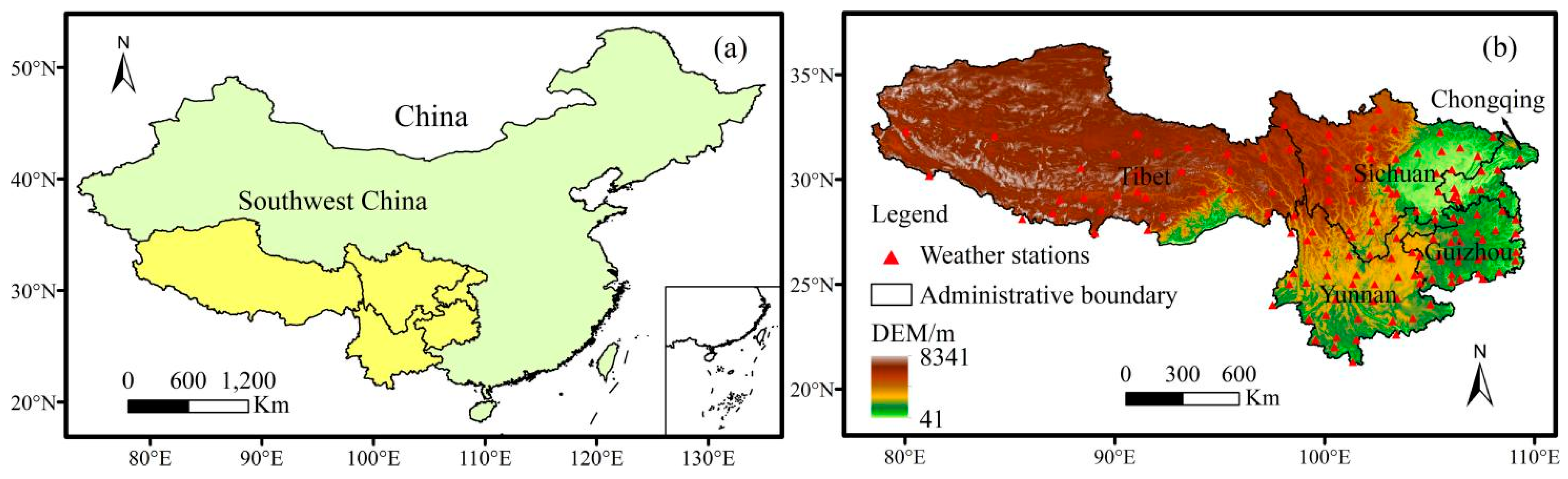
2.1. Study Areas
2.2. Data
2.2.1. Data Sources
2.2.2. Data Preprocessing
2.3. Methods
2.3.1. Calculation of Remote Sensing and Meteorological Drought Indices
2.3.2. ML Model
- (1)
- RF Model
- (2)
- XGBoost Model
- (A)
- XGBoost belongs to the category of rule-based models. Those models are generally better suited than DL algorithms for the datasets of moderate or small size.
- (B)
- XGBoost models have a higher accuracy due to the introduction of second-order Taylor expansion. The base learner of XGBoost can be a DT or a linear classifier, implying higher flexibility.
- (C)
- XGBoost models are convenient to build in that they can attain highly optimized performance by following a standard hyperparameter search process implemented using stratified k-fold nested cross-validation (CV). Because of the regularization term, XGBoost can also be easily trained in such a way as to reduce overfitting.
- (D)
- XGBoost can incorporate elements of cost-sensitive learning where a cost matrix can help influence the model to produce fewer false negatives.
- (E)
- XGBoost supports column sampling, and it can reduce computational load and accelerate the calculation. It has been used successfully to win several ML competitions.
- (F)
2.3.3. CV Method
2.3.4. Indicators of Model Accuracy Assessment
3. Results
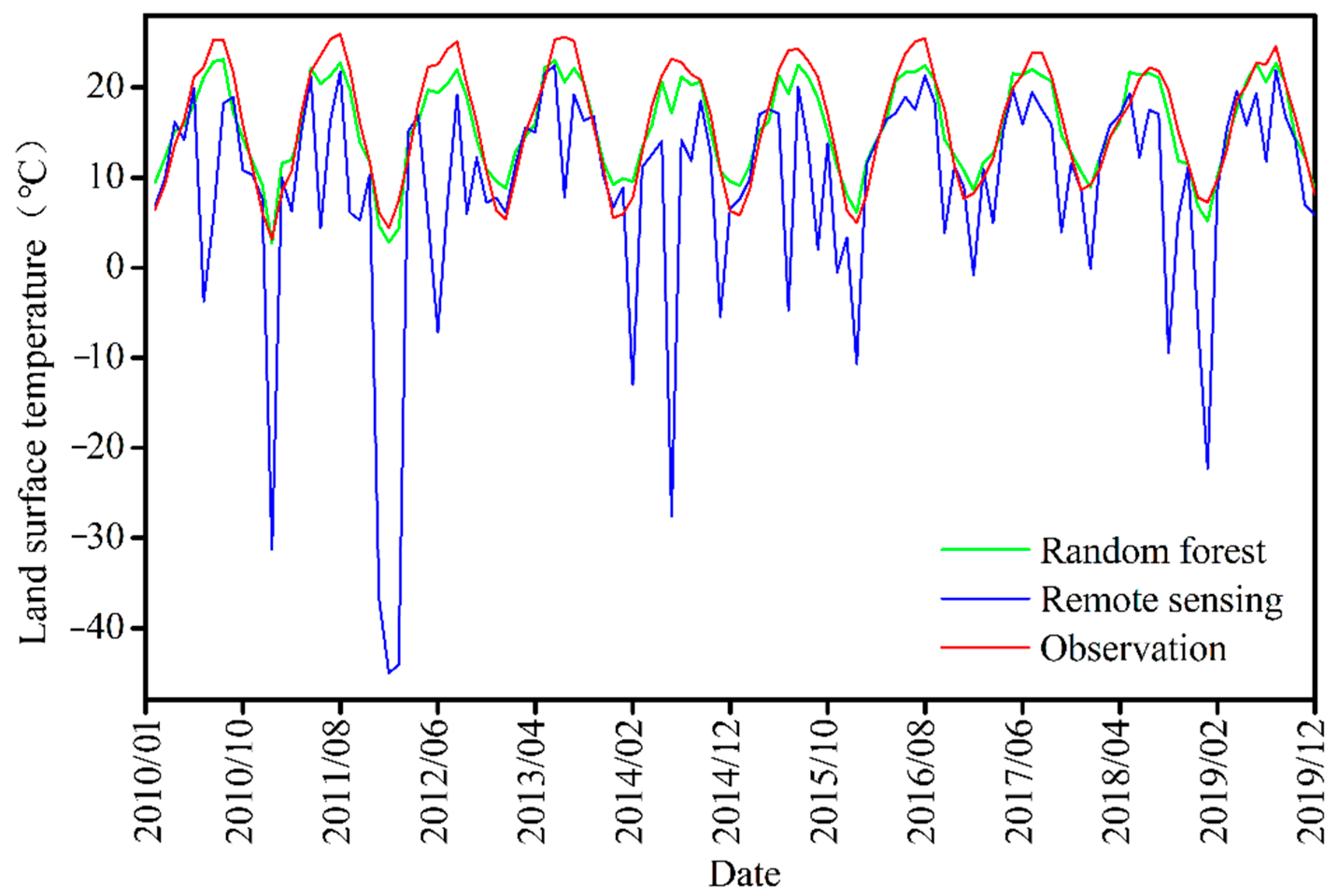
3.1. Reconstructing the LST Using an RF Model
3.1.1. Construction of an RF Model
3.1.2. Evaluation and Validation of Model Accuracy
3.2. Remote Sensing-Based Drought Monitoring Using XGBoost
3.2.1. Selection of Input and Output Parameters
3.2.2. Building a Remote Sensing-Based Drought Monitoring Model Using XGBoost
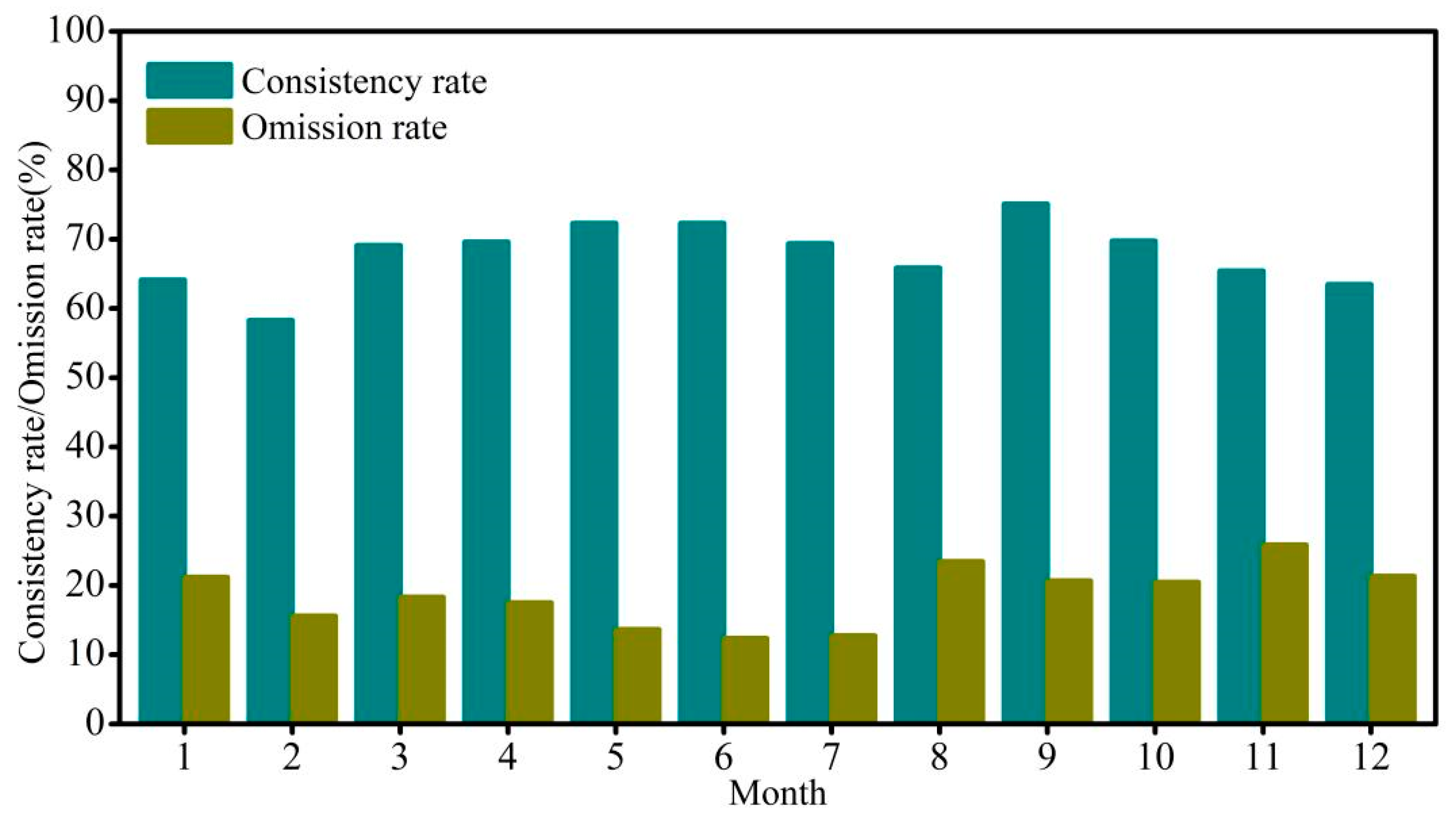
3.2.3. Model Accuracy Evaluation
4. Discussion
5. Summary and Conclusions
Author Contributions
Funding
Institutional Review Board Statement
Informed Consent Statement
Data Availability Statement
Conflicts of Interest
References
- Lemos, M.C.; Eakin, H.; Dilling, L.; Worl, J. Social Sciences, Weather, and Climate Change. Meteorol. Monogr. 2019, 59, 26.1–2625. [Google Scholar] [CrossRef]
- Vicente-Serrano, S.M.; Quiring, S.M.; Pena-Gallardo, M.; Yuan, S.S.; Dominguez-Castro, F. A Review of Environmental Droughts: Increased Risk under Global Warming? Earth-Sci. Rev. 2020, 201, 102953. [Google Scholar] [CrossRef]
- Masson-Delmotte, V.; Zhai, P.M.; Pirani, A.; Connors, S.L.; Péan, C.; Berger, S.; Huang, M.T.; Yelekçi, O.; Yu, R.; Zhou, B.Q. Climate Change 2021: The Physical Science Basis. In Contribution of Working Group I to the Sixth Assessment Report of the Intergovernmental Panel on Climate Change; IPCC: Geneva, Switzerland, 2021; Volume 2. [Google Scholar]
- Dai, A.G. Drought under Global Warming: A Review. Wiley Interdiscip. Rev. Clim. Chang. 2011, 2, 45–65. [Google Scholar] [CrossRef]
- Yuan, X.C.; Tang, B.J.; Wei, Y.M.; Liang, X.J.; Yu, H.; Jin, J.L. China’s Regional Drought Risk under Climate Change: A Two-stage Process Assessment Approach. Nat. Hazards 2015, 76, 667–684. [Google Scholar] [CrossRef]
- Jin, J.L.; Song, Z.Z.; Cui, Y.; Zhou, Y.L.; Jiang, S.M.; He, J. Research Progress on the Key Technologies of Drought Risk Assessment and Control. Shuili Xuebao 2016, 47, 398–412. [Google Scholar]
- Huang, J.P.; Chen, W.; Wen, Z.P.; Zhang, G.J.; Li, Z.X.; Zuo, Z.Y.; Zhao, Q.Y. Review of Chinese Atmospheric Science Research over the Past 70 Years: Climate and climate change. Sci. China Earth Sci. 2019, 49, 1514–1550. [Google Scholar] [CrossRef]
- Danandeh, M.A.; Rikhtehgar, G.A.; Yaseen, Z.M.; Sorman, A.U.; Abualigah, L. A Novel Intelligent Deep Learning Predictive Model for Meteorological Drought Forecasting. J. Ambient Intell. Humaniz. Comput. 2022, 14, 10441–10455. [Google Scholar] [CrossRef]
- Rahimi, B.S. Monitoring of Hydrological Drought in Khazar Basin. Watershed Eng. Manag. 2023. [CrossRef]
- Zhang, Q.; Yao, Y.B.; Li, Y.H.; Huang, J.P.; Ma, Z.G.; Wang, Z.L.; Wang, S.P.; Wang, Y.; Zhang, Y. Progress and Prospect on the Study of Causes and Variation Regularity of Droughts in China. Acta Meteorol. Sin. 2020, 78, 500–521. [Google Scholar] [CrossRef]
- Wang, Y.S.; Xiao, T.G.; Dong, X.F. Characteristics of Long-Cycle Abrupt Drought-Flood Alternations in Southwest China and Atmospheric Circulation in Summer from 1961, to 2019. Plateau Meteorol. 2021, 40, 760–772. [Google Scholar]
- Huan, D.B.; Fan, K.; Xu, Z.Q. Strengthened Relationship between Summer Barents Sea Ice and Autumn Southwest China Drought after the Mid-and Late-1990s. Trans. Atmos. Sci. 2022, 45, 167–178. [Google Scholar]
- Yao, Y.B.; Zhang, Q.; Wang, J.S.; Shang, J.L.; Wang, Y.; Shi, J.; Han, L.Y. The Response of Drought to Climate Warming in Southwest in China. Ecol. Environ. Sci. 2014, 23, 1409–1417. [Google Scholar]
- Yao, Y.B.; Zhang, Q.; Wang, J.S.; Shang, J.L.; Wang, Y.; Shi, J.; Han, L.Y. Temporal-spatial Abnormity of Drought for Climate Warming in Southwest China. Resour. Sci. 2015, 37, 1774–1784. [Google Scholar]
- Sun, Z.X.; Zhang, Q.; Sun, R.; Deng, B. Characteristics of the Extreme High Temperature and Drought and Their Main Impacts in Southwestern China of 2022. J. Arid Meteorol. 2022, 40, 764–770. [Google Scholar]
- Vicente-Serrano, S.M.; Beguería, S.; López-Moreno, J.I. A Multiscalar Drought Index Sensitive to Global Warming: The Standardized Precipitation Evapotranspiration Index. J. Clim. 2010, 23, 1696–1718. [Google Scholar] [CrossRef]
- Mi, Q.C. Construction and Prediction of the Ensemble Drought Index. Master’s Thesis, Shenyang Agricultural University, Shenyang, China, 2022. [Google Scholar]
- Guo, N.; Wang, X.P.; Wang, L.; Wang, L.J.; Hu, D.; Sha, S. Review of Drought Monitoring based on Remote Sensing Technology. Adv. Meteorol. Sci. Technol. 2020, 10, 10–20. [Google Scholar]
- Han, H.Z.; Bai, J.J.; Yan, J.W.; Yang, H.Y.; Ma, G. A Combined Drought Monitoring Index based on Multi-sensor Remote Sensing Data and Machine Learning. Geocarto Int. 2021, 36, 1161–1177. [Google Scholar] [CrossRef]
- West, H.; Quinn, N.; Horswell, M. Remote Sensing for Drought Monitoring & Impact Assessment: Progress, Past Challenges and Future Opportunities. Remote Sens. Environ. 2019, 232, 111291. [Google Scholar]
- Jiao, W.; Wang, L.; Mccabe, M.F. Multi-sensor Remote Sensing for Drought Characterization: Current Status, Opportunities and a Roadmap for the Future. Remote Sens. Environ. 2021, 256, 112313. [Google Scholar] [CrossRef]
- Qin, Q.M.; Wu, Z.H.; Zhang, T.Y.; Sagan, V.; Zhang, Z.X.; Zhang, Y.; Zhang, C.Y.; Ren, H.Z.; Sun, Y.H.; Xu, W.; et al. Optical and Thermal Remote Sensing for Monitoring Agricultural Drought. Remote Sens. 2021, 13, 5092. [Google Scholar] [CrossRef]
- Son, B.; Im, J.; Park, S.; Lee, J. Satellite-based Drought Forecasting: Research Trends, Challenges, and Future Directions. Korean J. Remote Sens. 2021, 37, 815–831. [Google Scholar]
- Li, Z. Drought Characteristics and Prediction Models in Northeast China. Ph.D. Thesis, Shenyang Agricultural University, Shenyang, China, 2021. [Google Scholar]
- Mullapudi, A.; Vibhute, A.D.; Mali, S.; Patil, C.H. A Review of Agricultural Drought Assessment with Remote Sensing Data: Methods, Issues, Challenges and Opportunities. Appl. Geomat. 2023, 15, 1–13. [Google Scholar] [CrossRef]
- Kogan, F.N. Application of Vegetation Index and Brightness Temperature for Drought Detection. Adv. Space Res. 1995, 15, 91–100. [Google Scholar] [CrossRef]
- Wan, Z.; Zhang, Y.; Zhang, Q.; Li, Z.L. Quality Assessment and Validation of the MODIS Global Land Surface Temperature. Int. J. Remote Sens. 2004, 25, 261–274. [Google Scholar] [CrossRef]
- Sandholt, I.; Rasmussen, K.; Andersen, J. A Simple Interpretation of the Surface Temperature/Vegetation Index Space for Assessment of Surface Moisture Status. Remote Sens. Environ. 2002, 79, 213–224. [Google Scholar] [CrossRef]
- Yin, Z.; Qin, G.; Guo, L.; Tang, X.; Wang, J.; Li, H. Coupling Antecedent Rainfall for Improving the Performance of Rainfall Thresholds for Suspended Sediment Simulation of Semiarid Catchments. Sci. Rep. 2022, 12, 4816. [Google Scholar] [CrossRef]
- Wu, Z.Y.; Cheng, D.D.; He, H.; Li, Y.; Zhou, J.H. Research Progress of Composite Drought Index. Water Resour. Prot. 2021, 37, 36–45. [Google Scholar]
- Krajewski, W.F.; Ciach, G.J.; McCollum, J.R.; Bacotiu, C. Initial Validation of the Global Precipitation Climatology Project Monthly Rainfall over the United States. J. Appl. Meteorol. 2000, 39, 1071–1086. [Google Scholar] [CrossRef]
- Shen, X.; Walker, J.P.; Ye, N.; Wu, X.; Brakhasi, F.; Boopathi, N.; Zhu, L.; Yeo, I.Y.; Kim, E.; Kerr, Y.; et al. Evaluation of the Tau-omega Model over Bare and Wheat-covered Flat and Periodic Soil Surfaces at P-and L-band. Remote Sens. Environ. 2022, 273, 112960. [Google Scholar] [CrossRef]
- Balti, H.; Abbes, A.B.; Mellouli, N.; Imed, R.F.; Sang, Y.F.; Lamolle, M. A Review of Drought Monitoring with Big Data: Issues, Methods, Challenges and Research Directions. Ecol. Inform. 2020, 60, 101136. [Google Scholar] [CrossRef]
- Park, S.; Im, J.; Jang, E.; Rhee, J. Drought Assessment and Monitoring Through Blending of Multi-sensor Indices using Machine Learning Approaches for Different Climate Regions. Agric. For. Meteorol. 2016, 216, 157–169. [Google Scholar] [CrossRef]
- Heydari, H.; Valadan, Z.M.J.; Maghsoudi, Y.; Dehavi, S. An Investigation of Drought Prediction Using Various Remote-sensing Vegetation Indices for Different Time Spans. Int. J. Remote Sens. 2018, 39, 1871–1889. [Google Scholar] [CrossRef]
- Shen, R.; Huang, A.; Li, B.; Guo, J. Construction of a Drought Monitoring Model Using Deep Learning Based on Multi-source Remote Sensing Data. Int. J. Appl. Earth Obs. Geoinf. 2019, 79, 48–57. [Google Scholar] [CrossRef]
- Cao, J.; Zhang, Z.; Tao, F.; Zhang, L.; Luo, Y.; Zhang, J. Integrating Multi-source Data for Rice Yield Prediction across China Using Machine Learning and Deep Learning Approaches. Agric. For. Meteorol. 2021, 297, 108275. [Google Scholar] [CrossRef]
- Sardar, V.; Chaudhari, S.; Anchalia, A.; Kakati, A.; Paudel, A.; Bhavana, B.N. Ensemble Learning with CNN and BMO for Drought Prediction. In Proceedings of the 2022 IEEE 3rd Global Conference for Advancement in Technology (GCAT), Bangalore, India, 7–9 October 2022; pp. 1–6. [Google Scholar]
- Kafy, A.A.; Bakshi, A.; Saha, M.; Faisal, A.A.; Almulhim, A.L.; Rahaman, Z.A.; Mohammad, P. Assessment and Prediction of Index Based Agricultural Drought Vulnerability Using Machine Learning Algorithms. Sci. Total Environ. 2023, 867, 161394. [Google Scholar] [CrossRef]
- Zhao, Y.Y.; Zhang, J.H.; Bai, Y.; Zhang, S.; Yang, S.S.; Henchiri, M.; Seka, A.M.; Nanzad, L. Drought Monitoring and Performance Evaluation based on Machine Learning Fusion of Multi-Source Remote Sensing Drought Factors. Remote Sens. 2022, 14, 6398. [Google Scholar] [CrossRef]
- Ali, S.; Khorrami, B.; Jehanzaib, M.; Tariq, A.; Ajmal, M.; Arshad, A.; Shafeeque, M.; Dilawar, A.; Basit, I.; Zhang, L. Spatial Downscaling of GRACE Data Based on XGBoost Model for Improved Understanding of Hydrological Droughts in the Indus Basin Irrigation System (IBIS). Remote Sens. 2023, 15, 873. [Google Scholar] [CrossRef]
- Dikshit, A.; Pradhan, B.; Santosh, M. Artificial Neural Networks in Drought Prediction in the 21st Century—A Scientometric Analysis. Appl. Soft Comput. 2022, 114, 108080. [Google Scholar] [CrossRef]
- Dikshit, A.; Pradhan, B. Interpretable and Explainable AI (XAI) Model for Spatial Drought Prediction. Sci. Total Environ. 2021, 801, 149797. [Google Scholar] [CrossRef]
- Ji, Y.H.; Zhou, G.S.; Wang, S.D.; Wang, L.X. Increase in Flood and Drought Disasters during 1500–2000, in Southwest China. Nat. Hazards 2015, 77, 1853–1861. [Google Scholar] [CrossRef]
- Fu, R.; Chen, R.; Wang, C.; Chen, X.; Gu, H.; Wang, C.; Xu, B.; Liu, G.; Yin, G. Generating High-Resolution and Long-Term SPEI Dataset over Southwest China through Downscaling EEAD Product by Machine Learning. Remote Sens. 2022, 14, 1662. [Google Scholar] [CrossRef]
- Mei, P.; Liu, J.; Liu, C.; Liu, J.N. A Deep Learning Model and Its Application to Predict the Monthly MCI Drought Index in the Yunnan Province of China. Atmosphere 2022, 13, 1951. [Google Scholar] [CrossRef]
- Zhang, Z.B.; Yang, Y.; Zhang, X.P.; Chen, Z.J. Wind Speed Changes and Its Influencing Factors in Southwestern China. Acta Ecol. Sin. 2014, 34, 471–481. [Google Scholar]
- Zhang, Q.; Li, Y.Q. Climatic Variation of Rainfall and Rain Day in Southwest China for Last 48 Years. Plateau Meteorol. 2014, 33, 372–383. [Google Scholar]
- Li, Q.; Wang, X.M.; Zhou, G.B.; Zhang, Y.P.; He, Y. Temporal and Spatial Distribution Characteristics of Short-time Heavy Rainfall during Southwest Vortex Rainstorm in Sichuan Basin. Plateau Meteorol. 2020, 39, 960–972. [Google Scholar]
- Zhang, Y.D.; Zhang, X.H.; Liu, S.R. Correlation Analysis on Normalized Difference Vegetation Index (NDVI) of Different Vegetations and Climatic Factors in Southwest China. Chin. J. Appl. Ecol. 2011, 22, 323–330. [Google Scholar]
- Zhao, Q.Q.; Zhang, J.P.; Zhao, T.B.; Li, J.H. Vegetation Changes and Its Response to Climate Change in China Since. Plateau Meteorol. 2021, 40, 292–301. [Google Scholar]
- Gruber, A.; Scanlon, T.; Robin, V.D.S.; Wagner, W.; Dorigo, W. Evolution of the ESA CCI Soil Moisture Climate Data Records and Their Underlying Merging Methodology. Earth Syst. Sci. Data 2019, 11, 717–739. [Google Scholar] [CrossRef]
- Dorigo, W.; Wagner, W.; Albergel, C.; Albrecht, F.; Balsamo, G.; Brocca, L.; Chung, D.; Ertl, M.; Forkel, M.; Gruber, A.; et al. ESA CCI Soil Moisture for Improved Earth System Understanding: State-of-the Art and Future Directions. Remote Sens. Environ. 2017, 203, 185–215. [Google Scholar] [CrossRef]
- Guo, X.; Yu, H.B.; Ma, Z.C.; Cao, C.M. Analysis of Spatial and Temporal Variations of Soil Moisture Content and Drought Degree based on MODIS. Resour. Soil. Water Conserv. 2019, 26, 185–189. [Google Scholar]
- Ma, H.X.; Chen, C.C.; Song, Y.Q.; Ye, S.; Hu, Y.M. Analysis of Vegetation Cover Change and Its Driving over the Past Ten Years in Qinghai Province. Resour. Soil. Water Conserv. 2018, 25, 137–145. [Google Scholar]
- GB/T 20481-2017; National Standard of the People’s Republic of China. Meteorological Drought Level. Standardization Administration of China: Beijing, China, 2018.
- Poornima, S.; Pushpalatha, M. Drought Prediction based on SPI and SPEI with Varying Timescales using LSTM Recurrent Neural Network. Soft Comput. 2019, 23, 8399–8412. [Google Scholar] [CrossRef]
- Zhao, J.P.; Zhang, X.F.; Liao, C.H.; Bao, H.Y. TVDI based Soil Moisture Retrieval from Remotely Sensed Data Over Large Arid Areas. Remote Sens. Technol. Appl. 2011, 26, 742–750. [Google Scholar]
- Wang, M.C.; Yang, S.T.; Dong, G.T.; Bai, J. Estimating Soil Water in Northern China based on Vegetation Temperature Condition Index. Arid. Land Geogr. 2012, 35, 446–455. [Google Scholar]
- Zhang, M.; Zhang, X.; Hu, G.C.; Wang, N. Applicability Analysis of Remote Sensing based Drought Indices in Drought Monitoring of Apple in Luochuan. Remote Sens. Technol. Appl. 2021, 36, 187–197. [Google Scholar]
- Li, X.H.; Mao, F.Y.; Wang, L.; Yang, J.K. Future Drought Projection of Southwestern China based on CMIP5 Model and MCI Index. In Proceedings of the 2021, 7th International Conference on Hydraulic and Civil Engineering & Smart Water Conservancy and Intelligent Disaster Reduction Forum (ICHCE & SWIDR), Nanjing, China, 6–8 November 2021; pp. 266–276. [Google Scholar]
- Breiman, L. Random Forests. Mach. Learn. 2001, 45, 5–32. [Google Scholar] [CrossRef]
- Park, S.; Im, J.; Park, S.; Rhee, J. Drought Monitoring using High Resolution Soil Moisture Through Multi-sensor Satellite Data Fusion over the Korean Peninsula. Agric. For. Meteorol. 2017, 237, 257–269. [Google Scholar] [CrossRef]
- Li, S.; Xu, X. Study on Remote Sensing Monitoring Model of Agricultural Drought based on Random Forest Deviation Correction. INMATEH-Agric. Eng. 2021, 64, 413–422. [Google Scholar] [CrossRef]
- Gu, Q.Y.; Han, Y.; Xu, Y.P.; Yao, H.Y.; Niu, H.F.; Huang, F. Laboratory Research on Polarized Optical Properties of Saline-alkaline Soil based on Semi-empirical Models and Machine Learning Methods. Remote Sens. 2022, 14, 226. [Google Scholar] [CrossRef]
- Bharathidason, S.; Venkataeswaran, C.J. Improving Classification Accuracy Based on Random Forest Model with Uncorrelated High Performing Trees. Int. J. Comput. Appl. 2014, 101, 26–30. [Google Scholar] [CrossRef]
- Chen, T.Q.; Guestrin, C. Xgboost: A Scalable Tree Boosting System. In Proceedings of the 22nd ACM SIGKDD International Conference on Knowledge Discovery and Data Mining, San Francisco, CA, USA, 13–17 August 2016; pp. 785–794. [Google Scholar]
- Xiao, Y.; Zhao, W.; Ma, M.; He, K. Gap-free LST Generation for MODIS/Terra LST Product Using a Random Forest-Based Reconstruction Method. Remote Sens. 2021, 13, 2828. [Google Scholar] [CrossRef]
- Cheng, Y.; Li, Y.X.; Wu, H.P.; Li, F.; Li, Y.Z.; He, L. Reconstructing Modis LST Products Over Tibetan Plateau based on Random Forest. In Proceedings of the IGARSS 2020-2020, IEEE International Geoscience and Remote Sensing Symposium, Waikoloa, HI, USA, 26 September–2 October 2020; IEEE: Piscataway, NJ, USA, 2020; pp. 6226–6229. [Google Scholar]
- Sun, M.; Gong, A.; Zhao, X.; Liu, N.; Si, L.; Zhao, S. Reconstruction of a Monthly 1 km NDVI Time Series Product in China Using Random Forest Methodology. Remote Sens. 2023, 15, 3353. [Google Scholar] [CrossRef]
- Zhao, W.; Duan, S.B. Reconstruction of Daytime Land Surface Temperatures under Cloud-covered Conditions Using Integrated MODIS/Terra Land Products and MSG Geostationary Satellite Data. Remote Sens. Environ. 2020, 247, 111931. [Google Scholar] [CrossRef]
- Wang, S.Y.; Zhang, Y.; Meng, X.H.; Song, M.H.; Shang, L.Y.; Su, Y.Q.; Li, Z.G. Fill the Gaps of Eddy Covariance Fluxes Using Machine Learning Algorithms. Plateau Meteorol. 2020, 39, 1348–1360. [Google Scholar]
- Chen, Y.; Ma, L.X.; Yu, D.S.; Feng, K.Y.; Wang, X.; Song, J. Improving Leaf Area Index Retrieval Using Multi-Sensor Images and Stacking Learning in Subtropical Forests of China. Remote Sens. 2021, 14, 148. [Google Scholar] [CrossRef]
- Zhang, R.; Chen, Z.Y.; Xu, L.J.; Ou, C.Q. Meteorological Drought Forecasting based on a Statistical Model with Machine Learning Techniques in Shaanxi Province, China. Sci. Total Environ. 2019, 665, 338–346. [Google Scholar] [CrossRef] [PubMed]
- Li, H.; Zhu, Y. Xgboost Algorithm Optimization Based on Gradient Distribution Harmonized Strategy. J. Comput. Appl. 2020, 40, 1633. [Google Scholar]
- Han, Y.X.; Wu, J.P.; Zhai, B.N.; Pan, Y.X.; Huang, G.M.; Wu, L.F.; Zeng, W.Z. Coupling a Bat Algorithm with Xgboost to Estimate Reference Evapotranspiration in the Arid and Semiarid Regions of China. Adv. Meteorol. 2019, 2019, 9575782. [Google Scholar] [CrossRef]
- Zhang, B.; Salem, F.K.A.; Hayes, M.J.; Simth, K.H.; Tadesse, T.; Wardlow, B.D. Explainable Machine Learning for the Prediction and Assessment of Complex Drought Impacts. Sci. Total Environ. 2023, 898, 165509. [Google Scholar]
- Babcock, C.; Finely, A.O.; Bradford, J.B.; Kolka, R.K.; Birdsey, R.A.; Ryan, M.G. LiDAR based prediction of forest biomass using hierarchial models with spatially varying coefficients. Remote Sens. Env. 2015, 169, 113–127. [Google Scholar] [CrossRef]
- Brenning, A. Spatial Cross-validation and Bootstrap for the Assessment of Prediction Rules in Remote Sensing: The R Package Sperrorest. In Proceedings of the 2012, IEEE International Geoscience and Remote Sensing Symposium, Munich, Germany, 22–27 July 2012; pp. 5372–5375. [Google Scholar]
- Cracknell, M.J.; Reading, A.M. Geological Mapping Using Remote Sensing Data: A Comparison of Five Machine Learning Algorithms, Their Response to Variations in the Spatial Distribution of Training Data and the Use of Explicit Spatial Information. Comput. Geosci. 2014, 63, 22–33. [Google Scholar] [CrossRef]
- Sharma, R.C.; Hara, K.; Hirayama, H. A Machine Learning and Cross-Validation Approach for the Discrimination of Vegetation Physiognomic Types Using Satellite Based Multispectral and Multitemporal Data. Scientifica 2017, 2017, 9806479. [Google Scholar] [CrossRef]
- Ramezan, A.; Warner, C.A.; Maxwell, T.E.A. Evaluation of Sampling and Cross-validation Tuning Strategies for Regional-scale Machine Learning Classification. Remote Sens. 2019, 11, 185. [Google Scholar] [CrossRef]
- Maxwell, A.E.; Warner, T.A.; Fang, F. Implementation of Machine-learning Classification in Remote Sensing: An Applied Review. Int. J. Remote Sens. 2018, 39, 2784–2817. [Google Scholar] [CrossRef]
- Duro, D.C.; Franklin, S.E.; Dubé, M.G. A Comparison of Pixel-based and Object-based Image Analysis with Selected Machine Learning Algorithms for the Classification of Agricultural Landscapes Using SPOT-5 HRG Imagery. Remote Sens. Environ. 2012, 118, 259–272. [Google Scholar] [CrossRef]
- Stone, M. Cross-validatory Choice and Assessment of Statistical Predictions. J. R. Stat. Soc. Ser. B (Methodol.) 1974, 36, 111–133. [Google Scholar] [CrossRef]
- Battineni, G.; Sagaro, G.G.; Nalini, C.; Amenta, F.; Tayebati, S.K. Comparative Machine-learning Approach: A Follow-up Study on Type 2 Diabetes Predictions by Cross-validation Methods. Machines 2019, 7, 74. [Google Scholar] [CrossRef]
- Shen, R.P.; Guo, J.; Zhang, J.X.; Li, L.X. Construction of a Drought Monitoring Model Using the Random Forest Based on Remote Sensing. J. Geo-Inf. Sci. 2017, 19, 125–133. [Google Scholar]
- Deng, J.H. Deep Learning—Principles, Models and Practice; Posts & Telecom Press: Beijing, China, 2021; pp. 47–50. [Google Scholar]
- Price, J.C. Using Spatial Context in Satellite Data to Infer Regional Scale Evapotranspiration. IEEE Trans. Geosci. Remote Sens. 1990, 28, 940–948. [Google Scholar] [CrossRef]
- Wang, R.J.; Li, X.H.; Zhou, R.J.; Wang, L. Applicability Analysis of Three Meteorological Drought Indices in Sichuan Province. Resour. Environ. Yangtze Basin 2021, 30, 734–744. [Google Scholar]
- Jia, H.J. Construction and Application of Remote Sensing Drought Monitoring Model based on Machine Learning in Southwestern China. Master’s Thesis, Chengdu University of Information Technology, Chengdu, China, 2022. [Google Scholar]
- Xie, W.S.; Zhang, Q.; Li, W.; Wu, B.Y. Analysis of the Applicability of Drought Indexes in the Northeast, Southwest and Middle-lower Reaches of Yangtze River of China. Plateau Meteorol. 2021, 40, 1136–1146. [Google Scholar]
- Duan, H.X.; Wang, S.P.; Feng, J.Y. The National Drought Situation and Its Impact and Causes in 2010. J. Arid Meteorol. 2011, 29, 126–132. [Google Scholar]
- Duan, H.X.; Wang, S.P.; Feng, J.Y. The National Drought Situation and Its Impact and Causes in the Summer of 2011. J. Arid Meteorol. 2011, 29, 392–400. [Google Scholar]
- Duan, H.X.; Wang, S.P.; Feng, J.Y. The National Drought Situation and Its Impact and Causes in 2011. J. Arid Meteorol. 2012, 30, 136–147. [Google Scholar]
- Chen, Y. Remote Sensing Retrieval of Soil Moisture Content Based on Ensemble Learning. Master’s Thesis, University of Electronic Science and Technology of China, Chengdu, China, 2020. [Google Scholar]
- Jia, Y.Q.; Zhang, B. Spatial-temporal Variability Characteristics of Extreme Drought Events based on Daily SPEI in the Southwest China in Recent 55 Years. Sci. Geogr. Sin. 2018, 38, 474–483. [Google Scholar]
- Wang, C.X.; Zhang, S.Q.; Chen, W.X.; Sun, R. Applicability and Revision of MCI in Sichuan Province. Chin. Agric. Sci. Bull. 2019, 35, 115–121. [Google Scholar]


| Type | Index | Formula | Note | Reference |
|---|---|---|---|---|
| Drought index calculated based on remote sensing information | NDVI | and are near-infrared and red bands, respectively. | [22] | |
| EVI | is the blue band; G, C1, C2 and L are empirical coefficients. | |||
| TRMM- SPI | SPI is calculated using the TRMM3B43 data. | [57] | ||
| VCI | NDVImin and NDVImax are the minimum and maximum values of the NDVI, respectively; the smaller the VCI, the more likely drought will occur. | [25] | ||
| TCI | LSTmax and LSTmin are the maximum and minimum values of LST, respectively; the smaller the TCI, the more severe the drought may be. | |||
| VTCINDVI | a1, b1, a2, and b2 are the regression equation coefficients of the dry and wet edge in the relationship between the NDVI and LST, respectively. The value ranges of the four indices are all between (0,1). Among these, the smaller the value of VTCINDVI and VTCIEVI, the more severe the drought may be, and the larger the value of TVDINDVI and TVDIEVI, the more severe the drought may be. | [22,34,58,59,60] | ||
| VTCIEVI | ||||
| TVDINDVI | ||||
| TVDIEVI | ||||
| VSWINDVI | The smaller the VSWINDVI and VSWIEVI, the more severe the drought may be. | |||
| VSWIEVI | ||||
| Drought index calculated based on meteorological station data | SPEI | ( (; | Calculated according to the Thornthwaite method recommended by Vicente-Serrano. p is the cumulative probability, W is the cumulative probability weighted moment, and c0, c1, c2, d1, d2, and d3 are all constant values. | [56] |
| MCI | Ka is the seasonal adjustment coefficient, SPIW60 is the standardized weighted precipitation index for the past 60 days, MI30 is the relative humidity index for the past 30 days, SPI90 is the SPI for the past 90 days, SPI150 is the SPI for the past 150 days, and a, b, c, and d are the weight coefficients of these indices. | [56,61] |
| Drought Grade | Type | SPEI/MCI Value |
|---|---|---|
| 1 | No drought | −0.5< |
| 2 | Mild drought | (−1.0, −0.5] |
| 3 | Moderate drought | (−1.5, −1.0] |
| 4 | Severe drought | (−2.0, −1.5] |
| 5 | Extreme drought | ≤−2.0 |
| Parameter | Meaning | Optimal Parameter |
|---|---|---|
| max_features | Maximum number of features used by a single decision tree | auto |
| max_depth | Maximum depth of the tree | 15 |
| min_samples_split | Minimum number of samples required to split a node | 2 |
| min_samples_leaf | Minimum number of samples contained in each leaf node | 1 |
| n_estimators | Number of decision trees to build | 537 |
| bootstrap | With or without put-back sampling | True |
| criterion | Evaluation criteria for segmentation quality | mse |
| Accuracy Assessment Indicator | Training Set | Testing Set |
|---|---|---|
| RMSE | 1.172 | 2.236 |
| MAE | 0.847 | 1.719 |
| EVS | 0.901 | 0.858 |
| CC | 0.944 ** | 0.908 ** |
| Drought Index | SM | TRMM-SPI | VCI | TCI | VTCINDVI | VTCIEVI | TVDINDVI | TVDIEVI | VSWINDVI | VSWIEVI |
|---|---|---|---|---|---|---|---|---|---|---|
| SPEI1 | 0.488 ** | 0.835 ** | 0.101 | 0.105 | 0.044 | 0.066 * | −0.097 | −0.071 | 0.187 | 0.096 * |
| SPEI3 | 0.499 ** | 0.568 ** | 0.096 | 0.090 | 0.021 | 0.004 | −0.083 | −0.064 | 0.105 | 0.078 |
| SPEI6 | 0.471 ** | 0.414 ** | 0.110 | 0.067 | 0.080 | 0.062 | −0.057 | −0.034 | 0.128 | 0.088 |
| Parameter | Meaning | Optimal Parameter |
|---|---|---|
| n_estimators | Number of submodels | 203 |
| max_depth | Maximum depth of the tree | 2 |
| learning_rate | Learning rate of the resulting model at each iteration | 0.06 |
| min_child_weight | Minimum number of samples contained in each leaf node | 2 |
| Subsample | Proportion of random sampling | 0.8 |
| Gamma | Controls whether to post-prune | 0 |
| colsample_bytree | Controls the proportion of each random sampling column | 1 |
| colsample_bylevel | Proportion of column sampling for each node splitting in each tree | 0.5 |
| reg_alpha | Weight of the L1 regularization term | 0.01 |
| eval_metric | Measures the validation data | mse |
| Accuracy Assessment Indicator | Training Set | Testing Set |
|---|---|---|
| RMSE | 0.135 | 0.435 |
| MAE | 0.095 | 0.328 |
| EVS | 0.976 | 0.782 |
| CC | 0.982 ** | 0.868 ** |
| Drought Grade | Number of Weather Stations with Consistent Drought Grade/Total Number of Weather Stations under Each Drought Grade | Consistency Rate (%) |
|---|---|---|
| Extreme drought | 91/339 | 26.84 |
| Severe drought | 712/1134 | 62.79 |
| Moderate drought | 1512/2077 | 72.80 |
| Mild drought | 1861/2624 | 70.92 |
| No drought | 10,624/11,106 | 96.87 |
| Total | 14,852/17,280 | 85.65 |
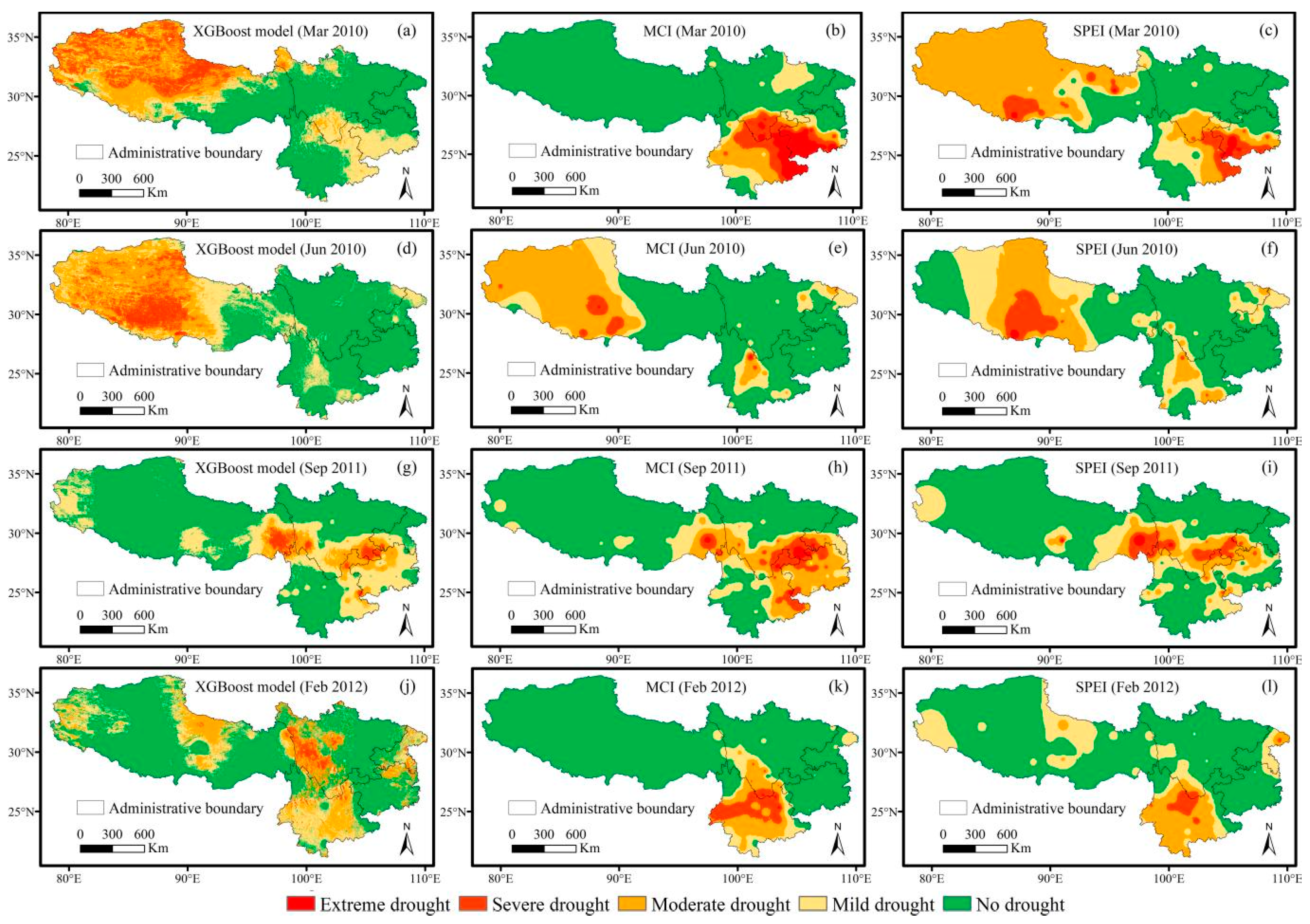
| Season\Region | Sichuan | Chongqing | Yunnan | Guizhou | Tibet |
|---|---|---|---|---|---|
| March 2010 | Mild-to-severe drought in the southern region during the first 10-day period, with the drought relieved during the third 10-day period | No apparent drought | Mild-to-severe drought in the southern region and extreme drought locally in the northern region during the first 10-day period with the drought relieved during the third 10-day period | Mild-to-severe drought in the southern region and extreme drought in the southwestern region during the first 10-day period with the drought relieved during the third 10-day period | Mild-to-severe drought in the central region with an extreme drought locally during the first 10-day period with the drought continuing into the third 10-day period |
| June 2010 | No apparent drought | No apparent drought | Moderate drought in the central region during the second 10-day period and a mild drought in the central and northern regions during the third 10-day period | No apparent drought | Mild-to-extreme drought in the central region, with an extreme drought mainly occurring near Nyima County of Nagqu City |
| September 2011 | Drought of moderate severity and above in the southeastern region, with a severe drought locally | Drought of moderate severity and above in the southwestern region, with a severe drought locally | Drought of moderate severity and above in the northeastern region with a severe drought locally | Drought of moderate severity and above in most regions with a severe drought in northwestern and eastern regions | Moderate-to-severe drought in central and eastern regions |
| February 2012 | Mild drought in the southwestern region during the first 10-day period with a moderate drought locally, and a severe drought in the central and western and southern regions during the third 10-day period | Moderate-to-severe drought in the central and northern regions | Mild drought in the western region during the first 10-day period, and a moderate-to-severe drought in most parts during the second 10-day period, with an extreme drought locally in the western region | No apparent drought | Mild-to-moderate drought in central and southern regions |
Disclaimer/Publisher’s Note: The statements, opinions and data contained in all publications are solely those of the individual author(s) and contributor(s) and not of MDPI and/or the editor(s). MDPI and/or the editor(s) disclaim responsibility for any injury to people or property resulting from any ideas, methods, instructions or products referred to in the content. |
© 2023 by the authors. Licensee MDPI, Basel, Switzerland. This article is an open access article distributed under the terms and conditions of the Creative Commons Attribution (CC BY) license (https://creativecommons.org/licenses/by/4.0/).
Share and Cite
Li, X.; Jia, H.; Wang, L. Remote Sensing Monitoring of Drought in Southwest China Using Random Forest and eXtreme Gradient Boosting Methods. Remote Sens. 2023, 15, 4840. https://doi.org/10.3390/rs15194840
Li X, Jia H, Wang L. Remote Sensing Monitoring of Drought in Southwest China Using Random Forest and eXtreme Gradient Boosting Methods. Remote Sensing. 2023; 15(19):4840. https://doi.org/10.3390/rs15194840
Chicago/Turabian StyleLi, Xiehui, Hejia Jia, and Lei Wang. 2023. "Remote Sensing Monitoring of Drought in Southwest China Using Random Forest and eXtreme Gradient Boosting Methods" Remote Sensing 15, no. 19: 4840. https://doi.org/10.3390/rs15194840
APA StyleLi, X., Jia, H., & Wang, L. (2023). Remote Sensing Monitoring of Drought in Southwest China Using Random Forest and eXtreme Gradient Boosting Methods. Remote Sensing, 15(19), 4840. https://doi.org/10.3390/rs15194840