Next Article in Journal
Contributions of Climate Variability and Anthropogenic Activities to Confined Groundwater Storage in Hengshui, North China Plain
Previous Article in Journal
GSDerainNet: A Deep Network Architecture Based on a Gaussian Shannon Filter for Single Image Deraining
Previous Article in Special Issue
Activities to Promote the Moon as an Absolute Calibration Reference
 
 
remotesensing-logo
Article Menu

Article Menu

Article

Towards Operational Fiducial Reference Measurement (FRM) Data for the Calibration and Validation of the Sentinel-3 Surface Topography Mission over Inland Waters, Sea Ice, and Land Ice

by
Elodie Da Silva
1,
Emma R. Woolliams
2,
Nicolas Picot
3,
Jean-Christophe Poisson
4,
Henriette Skourup
5,
Geir Moholdt
6,
Sara Fleury
7,
Sajedeh Behnia
2,
Vincent Favier
8,
Laurent Arnaud
8,
Jérémie Aublanc
9,
Valentin Fouqueau
4,
Nicolas Taburet
9,
Julien Renou
9,
Hervé Yesou
10,
Angelica Tarpanelli
11,
Stefania Camici
11,
Renée Mie Fredensborg Hansen
5,
Karina Nielsen
5,
Frédéric Vivier
12,
François Boy
3,
Roger Fjørtoft
3,
Mathilde Cancet
1,
Ramiro Ferrari
1,
Ghislain Picard
8,
Mohammad J. Tourian
13,
Nicolaas Sneeuw
13,
Eric Munesa
1,
Michel Calzas
14,
Adrien Paris
15,
Emmanuel Le Meur
8,
Antoine Rabatel
8,
Guillaume Valladeau
4,
Pascal Bonnefond
16,
Sylvie Labroue
9,
Ole Andersen
5,
Mahmoud El Hajj
1,*,
Filomena Catapano
17 and
Pierre Féménias
18
add Show full author list remove Hide full author list
1
NOVELTIS, 31670 Labège, France
2
NPL, National Physical Laboratory, Teddington TW11 0LW, UK
3
CNES, Centre National d’Etudes Spatiales, 31401 Toulouse, France
4
vorteX.io, 31670 Labège, France
5
DTU Space, National Space Institute, Technical University of Denmark, 2800 Kongens Lyngby, Denmark
6
NPI, Norwegian Polar Institute, 9296 Tromsø, Norway
7
LEGOS, Laboratoire d'Etudes en Géophysique et Océanographie Spatiales, 31400 Toulouse, France
8
IGE, Institut des Géosciences de l'Environnement, Université Grenoble Alpes, 38000 Grenoble, France
9
CLS, Collecte Localisation Satellites, 31520 Ramonville-Saint-Agne, France
10
SERTIT, Service Régional de Traitement d'Image et de Télédétection, 67000 Strasbourg, France
11
CNR-IRPI, Consiglio Nazionale delle Ricerche—Istituto di Ricerca per la Protezione Idrologica, 06100 Perugia, Italy
12
LOCEAN, Laboratoire d'Océanographie et du Climat: Expérimentations et Approches Numériques, 75005 Paris, France
13
GIS, Institute of Geodesy, University of Stuttgart, 70174 Stuttgart, Germany
14
DT-INSU, 29280 Plouzané, France
15
Hydro Matters, 31460 Le Faget, France
16
SYRTE, Observatoire de Paris—Université PSL, CNRS, 75000 Paris, France
17
Rhea Group, 00044 Frascati, Italy
18
ESA ESRIN, European Space Agency, 00044 Frascati, Italy
*
Author to whom correspondence should be addressed.
Remote Sens. 2023, 15(19), 4826; https://doi.org/10.3390/rs15194826
Submission received: 10 August 2023 / Revised: 25 September 2023 / Accepted: 29 September 2023 / Published: 5 October 2023

Abstract

:
The Copernicus Sentinel-3 Surface Topography Mission (STM) Land Altimetry provides valuable surface elevation information over inland waters, sea ice, and land ice, thanks to its synthetic aperture radar (SAR) altimeter and its orbit that covers high-latitude polar regions. To ensure that these measurements are reliable and to maximise the return on investment, adequate validation of the geophysical retrieval methods, processing algorithms, and corrections must be performed using independent observations. The EU-ESA project St3TART (started July 2021) aims to generalise the concept of Fiducial Reference Measurements (FRMs) for the Copernicus Sentinel-3 STM. This work has gathered existing data, made new observations during field campaigns, and ensured that these observations meet the criteria of FRM standards so that they can be used to validate Sentinel-3 STM Land Altimetry products operationally. A roadmap for the operational provision of the FRM, including the definition, consolidation, and identification of the most relevant and cost-effective methods and protocols to be maintained, supported, or implemented, has been developed. The roadmap includes guidelines for SI traceability, definitions of FRM measurement procedures, processing methods, and uncertainty budget estimations.

1. Introduction

The Copernicus Sentinel-3 Surface Topography Mission (STM), based on a constellation of two satellites, provides valuable surface topography and elevation information over a wide range of Earth surface types [1,2]. As well as measuring the sea surface topography and wave conditions, the mission provides valuable surface elevation information over inland waters, sea ice, and land ice, thanks to its synthetic aperture radar (SAR) altimeter (the SAR Radar Altimeter instrument; SRAL) which retrieves high-resolution along-track elevation measurements, and to its orbit that covers high-latitude polar regions [3,4]. In addition, new thematic products have been defined for Sentinel-3 altimetry measurements, enabling processing chains to be adapted to the surfaces observed.
The Copernicus Sentinel-3 STM must be adequately validated to ensure that the geophysical retrieval methods can be used with confidence [5]. The mission requirements traceability document (MRTD) [6] defines what an adequate validation involves. Validation requires a two-step approach. First, the uncertainties associated with the altimeter measurements, their corrections, e.g., for atmospheric and geophysical phenomena, and the processing algorithms must be considered. Second, these uncertainties should be validated through comparison with independent observations, which themselves have strong traceability to the international system of units, the SI.
The decisions in designing a set of independent observations to be compared with the satellite product depend on surface type. These comparisons can be performed through the use of a field campaign based on a single satellite overpass or using permanent or semi-permanent stations, taking continuous measurements for longer periods of time. They can use other remote methods (e.g., from an aircraft, unmanned aerial vehicles (UAVs), or other satellites) or in situ methods in contact with the surface. Aside from the uncertainties associated with the independent measurements themselves, there are also uncertainties associated with translating the independent measurements (local measurand) into the Sentinel-3 STM product (satellite measurand), i.e., how to perform the spatial transformation between the ground (or in air or on/below water) measurements and the satellite observations.
The validation of satellite altimetry products has traditionally relied on a wide range of approaches that have been independently developed by different communities. This means that for traditional approaches there are a wide range of different procedures for making and comparing measurements and different levels of uncertainty evaluation and traceability. The concept of Fiducial Reference Measurements (FRMs) [7] presents an opportunity to standardise and enhance the validation process. The FRM framework provides a set of guidelines that instil the necessary confidence in the validation of satellite products.
FRMs are a suite of “independent, fully characterised, and traceable (to a community-agreed reference, ideally the SI) measurements, tailored specifically to address the calibration/validation needs of a satellite borne sensor and that follow the guidelines outlined by the GEO/CEOS Quality Assurance framework for Earth Observation (QA4EO)” [8]. QA4EO was endorsed by the Committee on Earth Observation Satellites (CEOS) in 2010, as part of the Group on Earth Observation (GEO) efforts to build an interoperable ‘system of systems’ for Earth observation data.
The St3TART project (Sentinel-3 Topography Mission Assessment through Reference Techniques), co-funded by the ESA and the EU [1,2] Copernicus Program, aimed to prepare a roadmap in view of the operational provision of FRMs to support the validation activities and foster the exploitation of the Sentinel-3 SAR altimeter land data products over inland waters, sea ice, and land ice areas [9]. This paper presents a synthesis of the protocols defined within St3TART for the Cal/Val of the Sentinel-3 Topographic Mission over those surfaces and details the need for FRM data within these activities and a roadmap for future work.
In this paper, Section 2 discusses what the requirements are for measurements to be considered as FRMs and describes the opportunities and challenges for FRMs over different surfaces. Section 3 describes the methodology for the St3TART project, which includes reviewing existing approaches and performing some field campaigns, as well as establishing a webportal for data dissemination. Section 4 collates some results from this analysis and defines a strategy for developing FRMs over each surface type. Section 5 presents recommendations for a roadmap of how FRMs can be established.

2. Requirements for FRMs for S3 Topography Products

This work explores the opportunities to provide FRM datasets for the calibration and validation of surface topography thematic data products for inland waters, land ice, and sea ice. First, in this section, we consider what is required for an in situ or airborne dataset to be considered FRM and present the concept of FRM approaches for different surfaces. We also present how such datasets can be made available to a broad user community through a central data hub.

2.1. FRMs as QA4EO References

Goryl et al. [7] indicate a set of ‘mandatory defining characteristics’ for a measurement set to be considered to be an ‘FRM’. These requirements are designed to ensure the stability of the non-satellite observations, to support robust uncertainty assessment (including error correlation structures), and to ensure that the uncertainty associated with transforming the measurand to match the satellite observation is considered. These defining characteristics are established to ensure that ‘FRMs’ comply with the core QA4EO principle that “data and derived products are easily accessible in an open manner and have an associated indicator of quality traceable to reference standards (preferably SI) so users can assess suitability for their applications, i.e., ‘fitness for purpose’”. Since 2010, several projects have established guidelines for how to apply metrological principles to FRMs and to the satellite data themselves [10], and these guidelines are available on the QA4EO website [8].
While QA4EO recognises that SI traceability may not be feasible for all measurements, the accompanying guidelines are based on metrological concepts and strongly imply a metrological approach. Metrology, the science of measurement, is the discipline responsible for ensuring that SI units are stable over centuries, internationally consistent, and coherent. These benefits are realised through traceability, and the central tenets are comparison and uncertainty analysis. This means that for FRMs, their traceability to references shall be documented and understood, and uncertainties are to be propagated through that traceability chain: from laboratory calibrations of instruments, through the uncertainties associated with field measurements, to the uncertainties inherent in converting the instrument measurand to the satellite measurand and those associated with any averaging or otherwise combining data from different times and spatial positions. Furthermore, FRMs themselves should be validated through comparisons between them, or between different instruments at an FRM site.
Note that the term ‘FRM’ can be used both for the measurements (data points) themselves, and for the infrastructure established (i.e., the instruments and processing chain). It can also be used both for measurements that support the ‘fundamental data record’ from the satellite (level 1 or early level 2 data) and measurements that support ‘thematic data products.’ In this paper, we consider Sentinel-3 STM thematic data products, as described in Section 2.3.2.

2.2. Applying a Metrological Approach to Uncertainty Analysis

A metrological uncertainty analysis involves five steps. The first, and arguably most important and difficult, is identifying the measurand(s) of interest, as well as identifying the measurement model: an analytical function that describes how the measurand is calculated from more fundamental ‘input quantities.’ The second step defines the route to traceability. It can help to document this with equations, and in diagrams. The third step is to document what is known about each (non-negligible) source of uncertainty. This will include the magnitude of the standard uncertainty, its probability distribution function, and information about how the uncertainty in that input quantity is converted to uncertainty in the main measurand, through sensitivity coefficients. As well as this, it is important to consider how the unknown error due to that source of uncertainty may be correlated between different measurements at different times or in different locations (i.e., in what ways the unknown errors are ‘systematic’ or ‘random’ in different dimensions). The fourth step is to calculate the measurands and their associated uncertainties. Uncertainty propagation should be performed according to the principles of the Guide to the Expression of Uncertainty in Measurement [11] and can use either the law of propagation of uncertainties, which approximates the uncertainty propagation using locally linear Taylor series expansion, or Monte Carlo methods, which approximate the uncertainty propagation via statistical means and by sampling the uncertainty distributions. Monte Carlo methods can cope with more sophisticated measurement functions; however, they are computationally expensive and may not be possible for very large datasets. Finally, in the fifth step, the uncertainty information should be stored for long-term data preservation purposes, so that future scientists can understand the detail of what has occurred and disseminate it, usually in summary form, for today’s users.

2.3. FRMs in Comparison with Satellite Data

2.3.1. Purpose and Types of Comparisons

The purpose of the FRM is to support the calibration and validation of the satellite altimeter observational datasets by providing non-satellite (in situ and ground-based aircraft and shipborne remote sensing techniques) references for comparisons. From a conceptual perspective, the results of such comparisons could be interpreted in three different ways:
(a)
To validate that observation values are within an expected tolerance;
(b)
To evaluate the uncertainty associated with the satellite observation;
(c)
To validate independently determined uncertainties.
Traditionally, comparisons have been used for approach (a), i.e., to monitor whether satellite and reference measurements agree within the stated satellite ‘absolute accuracy’ requirements, a term that is intended to specify an acceptable bias to agreed references. Approach (b) relies on the (usually unjustified) assumption that non-satellite measurements have negligible uncertainty compared to satellite observations and that any transfer or representation uncertainty in converting from the non-satellite measurand to the satellite measurand is also negligible.
A fully metrological approach would follow approach (c), described above. All uncertainties associated with the comparison would be independently determined and then validated through the comparison. These uncertainties would include those associated with the satellite altimeter observations, those associated with the measurements made by the FRM instruments, and those associated with transforming the non-satellite measurements to match the measurand of the satellite—i.e., transferring measurements in time and space. In such an analysis, the error correlation structures (i.e., systematic/random behaviour in time and space) should also be considered.

2.3.2. Satellite Thematic Data Product (TDP)

A metrological approach starts with defining the measurand and, because it is the purpose of an FRM to provide validation of the satellite data product, a metrological approach to an FRM must start by understanding the satellite’s measurand. Satellite datasets are processed through several stages to obtain a series of different measurands, usually moving from a raw measured signal up to a geophysical product of interest. There can be benefits of providing an FRM comparison for the different satellite measurands at different stages of this processing.
The most basic product provided by the European Space Agency (ESA) (as with other space agencies) is the level 1 dataset [12], known by the ESA as the ‘fundamental data record’ (FDR) if it follows QA4EO principles itself [13]. This is processed from the truly raw data of level 0. For SRAL, the level 1B products contain geolocated, multi-looked, and fully calibrated high-resolution power echoes that come from the unfocused SAR processing, with an along-track resolution of 320 m or 450 m, depending on the processing used. FRM approaches for level 1 are based on transponder measurements [14]. In level 2 processing, from the radar echoes, the range measurement is computed using a retracking algorithm which aims to estimate the time when the echo is received (epoch) inside a window and add this to the window delay (an instrumental parameter corresponding to the time when the acquisition window starts) [15]. As each surface leads to a different type of SAR echo, a different retracking algorithm is needed for each surface. This range is then subtracted from the orbital height and corrections are applied to account for atmospheric delays and geophysical phenomena such as tides. The uncertainty in range estimation is, consequently, directly linked to the quality of epoch estimation and to the retracking algorithm used. Geophysical and environmental corrections and their associated uncertainties may be evaluated in different ways. The outcome of this is the surface height, which is itself further processed to obtain the desired ‘thematic data products’ (TDPs): higher level satellite data that follow QA4EO principles.
For inland waters and land ice, the standard retracker currently used is the OCOG retracker [16], which is an empirical retracker that computes the epoch from the centre of gravity of the power integral of the radar echo. This approach has significant limits, especially where there are multi-peak echoes, and physical-based retracking models are under development. These physical-based models consider the specular nature [17] of the returned signal over small inland water bodies, and/or the penetration in the media (over land ice). Whatever retracker is used, it is also important to note that the satellite track varies from orbit to orbit. Over a large lake, this is dealt with by defining a virtual station as a larger area over which the lake surface is considered an equipotential surface and therefore different tracks can be combined. Over rivers, a choice can be made between creating a similar virtual station and correcting individual tracks to a particular position using a model of the height variation in the river between the tracks and the virtual station, or by providing the specific track position as part of the satellite dataset.
Ice sheets have complex terrains with significant surface undulations and slopes, varying from gentle slopes and variable roughness in the inland to higher slopes and rougher terrain along the coast, sometimes including a flatter floating part known as ice shelves. Such complex surfaces can result in complex returned echo waveforms with multiple peaks. Most commonly, the first reflection is used to identify the ‘point of closest approach’ (POCA) to the satellite. The geolocation of POCA will depend on the surface topography and can deviate by several kilometres from the satellite nadir ground track. Since the satellite orbits vary by several hundred metres between different overpasses, the repeated POCA tracks deviate even more due to the additional impact of variable topography. The TDP therefore consists of both the slant-corrected POCA range and its geolocation. For both land ice and sea ice, additional complexity comes from the fact that the Ku-band radar penetrates and scatters within the top snow layer, both slowing the return signal and providing a different reference to what is measured using other techniques, such as laser altimetry.
For sea ice, the primary objective is to derive the sea ice thickness. Here, as shown in Figure 1, the principle is that radar signals can discriminate between ice floes and leads (fractures in sea ice, where calm ocean water occurs) based on the shape of the returned radar echo [5,18,19,20]. From this discrimination of observations, the differences between the retracked surface height anomalies originating from floes and leads (interpolated into the floe observations) are computed [20,21,22,23]. This difference is denoted as the radar freeboard (height of sea ice above local water level). The radar freeboard is further processed to account for the radar penetration in the snow layer above the ice, which slows the signal, to give the sea ice freeboard [24]. The sea ice thickness is then determined by considering the buoyancy of the ice (from the densities of ice and sea water) and accounting for the weight of snow (depth and density) that is not measured by the radar.

2.3.3. Overview of FRM Requirements for the Different Surfaces

Inland water observations include those over large lakes, where the altimeter data are similar (but not identical) to ocean waters and smaller lakes and rivers, which require separate dedicated processing [25,26]. The open loop tracking of SRAL has enabled far smaller water bodies to be measured, bringing a new era of inland waters to satellite altimetry [27]; however, signal contamination from the surrounding land is still often challenging, as discussed in the previous section. For inland waters, permanent stations have been established to monitor the long-term temporal variability of the water surface. Nevertheless, these permanent stations, often supported by existing structures such as bridges and piers, are rarely at the exact location of the satellite nominal overpass, considering in addition that the actual overpass fluctuates from orbit to orbit. Comparisons are instead made to a ‘virtual station’, which is an area on a lake where the height is averaged, or a position on a river where all measurements, from satellite or other approaches, can be corrected to those in [28]. Such a translation is based on a river profile, or a lake profile, obtained during field campaign measurements using boats, UAVs, or aircraft.
Sea ice thickness observations are based on altimeter measurements of ice floes and leads, as shown in Figure 1, with corrections to account for snow and the buoyancy of the ice. Independent measurements can be made to be compared with the satellite for each step of the processing chain: the airborne radar can be compared with the radar freeboard [29], other airborne [30] and in situ [31,32] methods can be used to validate sea ice freeboard and sea ice thickness, and submarine measurements [33], which provide sea ice draft (the part of the sea ice below the water surface) measurements, can also be converted into sea ice thickness measurements. Currently, the only permanent stations for sea ice observations are ocean moorings continuously measuring the sea ice draft with upward-looking sonar at a fixed point in space [34,35,36,37]. Due to the continuous movement of sea ice, the time averaged sea ice draft will thus provide a spatial average of the ice pack. Semi-permanent stations can be installed in buoys embedded in, and moving with, the sea ice [34,38,39]; such observations will provide continuous measurements following the same ice floe and will not provide spatial variations in the ice pack unless multiple buoys are deployed in an array. Aircraft campaigns are also important for sea ice product validation [40].
For land ice, satellite altimetry is used for two complementary purposes: either to generate or georeference a digital surface model (DSM) for the ice surface (e.g., [41,42]) or to monitor changes in surface elevation over time (e.g., [43,44]). For DSM applications, a widespread coverage of data is needed over a period short enough that the snow/ice surface will not have changed significantly. For surface elevation changes, it is important to monitor the same locations repeatedly over long time periods. Radar altimetry data over land ice can be hard to interpret when there are complex surface variations within the signal footprint. Over such surfaces, the returned waveforms can have a complex set of peaks and be affected by penetration in the medium. Independent reference measurements can be collected in airborne or snow vehicle campaigns or from semi-permanent stations on the ice. Such stations can be sensitive to drifting snow and other temporary changes, and need to be precisely georeferenced, accounting for topography.

2.3.4. Types of FRM

The FRM consists of observations from instruments that are independent of the satellite observations and their processing, that can be compared with the satellite. In general, the FRM observations cannot themselves be directly compared with the satellite measurand but must be transformed to be comparable.
FRMs can consist of permanent, semi-permanent, or campaign-based observations. Long-term data series from permanent stations may be supplemented by campaign-based observation to determine the surface profile between the location of the fixed station and the point of satellite overpass. For land ice, the in situ observations made are not entirely permanent as the devices are mounted on ice that slowly moves. This movement is far more pronounced with the constantly changing sea ice surface. These long-term observations are conducted as the equipment floats with the ice or observes ice moving past. For both ice campaigns, using aircrafts, UAVs, or moving platforms on the surface is extremely important.
Most FRM techniques are based on forms of remote sensing: using radar, lidar, or ultrasound measurements to determine distances to the surface. These relative measurements also require knowledge of the position of the platform, whether that is mounted to a bridge over a river, fixed above the ice, or on an aircraft or other moving structure. The platform position is generally measured using a Global Navigation Satellite System (GNSS) receiver. Sometimes, contact methods can be used where the GNSS is in contact with the surface, for example, mounted on a raft pulled behind a boat or sled. There is considerable synergy on the FRM techniques used on the different surfaces, and thus there are advantages of considering the different FRMs as part of an overall system of systems.

2.3.5. Establishing the Measurand from the FRM Observations for Comparison

In general, with an FRM, the FRM observations need to be transformed (translated) to match the satellite product measurand. The satellite measurand for these thematic products is not necessarily the 20 Hz height measurements. As discussed in previous sections, it may be the average height in a virtual station defined on a lake, the average sea ice thickness, or a set of geolocated POCA measurements over land ice. Figure 2 schematically shows how the FRM observations are transformed to match the satellite product measurand. The diagram shows how the nadir satellite track (black dotted line) passes over all of the types of sites considered in this paper. Note that the satellite track can move several hundred metres from one satellite overpass to the next. The satellite product measurand, as shown from bottom to top, includes an area average over a lake virtual station (yellow circle), an SAR footprint over an extended river and sea ice (pink rectangle), where the latter is converted to a freeboard, and POCA measurements (blue dots) over land ice. The FRM measurements, shown as campaigns in green or as fixed stations by grey diamonds, must be transformed in space and time to match the satellite observations, and may also be averaged. In moving surfaces, particularly sea ice, surface drift must also be taken into account.
Over lakes, the FRM comparison is performed against a satellite product measurand that is the average water height within the virtual station. Campaign measurements (from a UAV or a raft behind a boat) can be used to determine an FRM value for the average height within the virtual station at the time of the campaign. Data from a fixed station can be used to provide a time series of this value, where the fixed station is either within the virtual station or close by.
Over a river, the FRM needs to be translated to the location of the satellite overpass or a defined virtual station. This spatial transfer must compensate for the river slope, which has been previously determined through a UAV or boat campaign measurement along the relevant stretch of river. Such campaigns must be performed for different river conditions at different times of year. For highly dynamic rivers, a temporal transfer may also be needed to account for variations in the river profile over time and the time it takes for the water to move from the FRM station to the satellite overpass point.
Over sea ice, the different product measurands (radar freeboard, ice freeboard, sea ice thickness) require different FRM instruments and thus different approaches for transferring the FRM to the satellite measurand. Airborne campaigns (from aircraft or drones) can be used to provide a large-scale profile of the sea ice and leads at a particular time. When a Ku-band radar is mounted on the aircraft, it measures the radar freeboard in the same way as Sentinel 3. With a Ka-band radar or lidar on the aircraft, the total freeboard is measured, or in the case of Ka-band, a freeboard close to the total freeboard depending on the snow conditions, as it might experience penetration into the top of the snow layer. Ice buoys, embedded within the sea ice for a season, and ice breaker ship measurements can be compared to the sea ice thickness satellite product. Finally, an upward-looking sonar measurement of sea ice draft can be processed to sea ice thickness with a similar analysis to how freeboard is processed (terms are as defined in Figure 1). In translating and transforming these FRM measurements to the satellite product measurand, corrections are needed to account for the movement of the sea ice. In many cases, this movement is dealt with through large-scale area and temporal averaging. Where point-to-point comparisons are used, the sea ice motion must be corrected for.
Over land ice, the satellite observations are geolocated at the POCA (blue dots in Figure 2). Within a region of interest (yellow circle), a local DSM is produced during a field campaign, which can be used to transfer the measurements at the fixed station to those at the POCA for any specific satellite observation. Comparisons are typically averaged within the region of interest. Field campaigns for generating the DSM can typically only be performed in the Antarctic summer or Arctic spring, and assumptions must be made that the relative topography only changes randomly between field campaigns.

3. Methodology

3.1. St3TART Project Approach

The first phase of the St3TART project had the aim of preparing a roadmap for operational provision of FRMs for the inland water, sea ice, and land ice products from Sentinel-3. This involved reviewing existing independent (non-satellite) measurements and measurement campaigns through a literature review, installing instruments, and/or performing prototype measurement campaigns, which included considering the processing of data from an FRM and what transformations are required to convert the FRM measurement into the measurand of the Sentinel-3 satellite, and performing the initial stages of an uncertainty budget, including identifying key sources of uncertainty and showing the metrological traceability of the observations. The results of the literature reviews and prototype measurements were used in each case to categorise different FRM options.
Because each surface had different scientific and practical challenges, the different teams emphasised these different aspects in different ways. The inland water team focused on establishing a small number of prototype ‘supersites’ on European rivers (see Section 4.1) with instruments and field campaigns to correct for river topography in comparison with the satellite observations. The sea ice team focused on field campaigns to demonstrate the ability of drone-borne lidar instruments in the harsh Arctic environment. The land ice team collated data from existing instrumentation and previous field campaigns to make a prototype quantitative uncertainty assessment.
All of these efforts should be seen as the first step towards operational FRM provision and considerable additional work is needed. This work was identified in the different roadmaps (see Section 5).

3.2. Disseminating FRM to Users

It is important to ensure that FRM measurements, and their associated documentation, providing traceability and uncertainty analysis, are available to the Cal/Val community in a free and accessible manner. To enable this to happen, a website has been established, with a user-friendly interface, permitting sharing FRM measurements with the community: the FRM Data Hub, which is accessible to the public at the following URL: https://frm-datahub.noveltis.fr/ (accessed on 3rd October 2023). All users can see available data, but to download data, registration is needed.
To facilitate the integration of new datasets in the database, a format specification document has been produced, describing the filename convention and the metadata of the datasets. The chosen format is NetCDF, as NetCDF files are ubiquitous in Earth sciences and therefore fully supported by a wide array of software solutions (QGIS, Panoply, ncview, nco, cdo, etc.) and libraries in most common languages (Fortran, C/C++, Python, Java, etc.). In addition, the format specification document lists the global attributes and the variable attributes that are needed or optional for the FRM Data Hub. Through the website, a user can browse data, filter data by surface type, time period, geographic area, type of sensor, or provider, and then select measurements and visualise the associated metadata, before downloading any dataset of interest.
The format specification document also specifies the way to distribute uncertainty variables: there shall be at least one uncertainty variable per variable, with an uncertainty value per observation point. Ideally, the different sources of uncertainties shall be distinguished. To take this into account, 3 uncertainty variables can be defined:
  • variable_standard_name_uncertainty_systematic: to cover uncertainties associated with effects that lead to errors that are common from observation to observation.
  • variable_standard_name_uncertainty_random: to cover uncertainties associated with effects that lead to errors that are independent from observation to observation.
  • variable_standard_name_uncertainty_structural: to cover uncertainties associated with errors that vary in ways between ‘systematic’ and ‘random’.
The variable attributes of the uncertainty variables shall give a link towards a document describing how uncertainties have been calculated.
It is also important to ensure the “operational aspect” of data provision. The Sentinel-3 Land STM Mission Performance Cluster (MPC) has requirements on the timeliness of measurements, e.g., validation data shall be available within 2 days after the measurement for hydrology Short Time Critical (STC) products. This means that some processes must be defined to operationalise the production and distribution of FRMs. The FRM Data Hub shall then offer interfaces such as FTP or API, to enable providers to push their FRM data automatically to users as soon as they are produced. Of course, FRMs with longer timeliness are also welcomed, especially for research activities and climate studies.

4. Results for Prototype Cal/Val Altimetry Protocols for Inland Waters, Sea Ice, and Land Ice

In this section, we summarise the reviews of existing non-satellite observations that are made over the different surface types and the results of the prototype activities.

4.1. Inland Waters

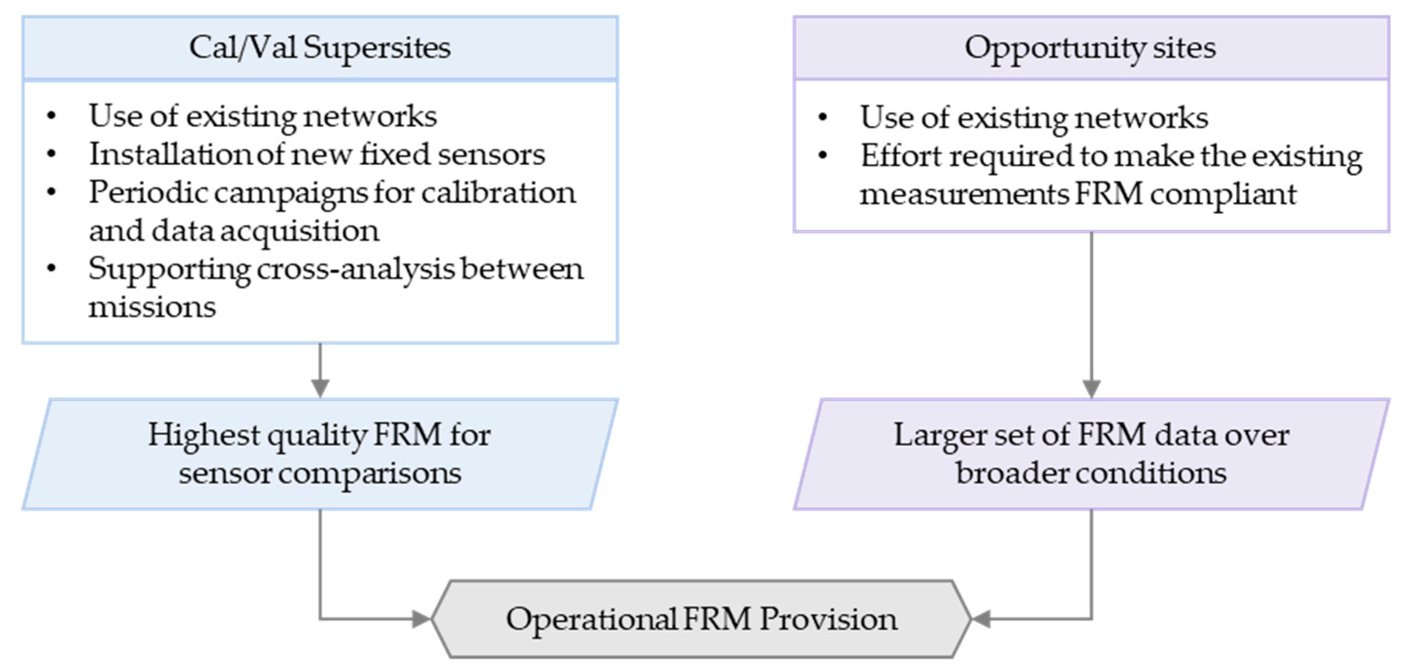
4.1.1. Strategy for Operational FRM Provision over Inland Waters

An approach towards FRM provision over inland waters has been explored and prototyped. The MRTD [6] describes the need for references over large rivers, their tributaries, and lakes. The approach involves (a) the development of new so-called ‘Cal/Val supersites’ that are established as FRM sites, which may be new, or building on existing sites, and (b) taking advantage of existing networks of in situ sensors, considered to be ‘opportunity sites.’
For rivers, the proposed supersites allow the analysis of watercourses of different widths, with simple (canal) and complex topography, and slow or dynamic temporal variations, with different measurement geometries (from perpendicular to parallel to Sentinel-3 track) and different cross-track distances (analysis of the off-nadir capabilities). These supersites are categorised according to how complex the transformation of the FRM measured values into the Sentinel-3 measurand is. The sites established in the first phase of the project are considered as examples and should be completed by other supersites that follow FRM approaches.
In addition to the supersites that are chosen for their situation and variety, we encourage the use of ‘opportunity sites’. These take advantage of existing in situ networks, and can be supplemented with additional efforts (e.g., uncertainty assessment, additional measurements) to meet the FRM requirements when possible. The resulting FRM provisioning strategy scheme is presented in Figure 3.

4.1.2. Supersites for Inland Waters

Altimeter measurements of rivers are complex and dynamic, especially with rivers with considerable slopes. The surface roughness can evolve drastically on a river or a lake depending on wind conditions and the surrounding terrain, modifying the radar return strongly and creating errors of several centimetres or decimetres. In addition, as the position of the satellite track moves from cycle to cycle within ±1 km of the reference ground track, the POCA will also move from cycle to cycle according to the position of the track and the variation in the slope/landform of the river. This means that for supersites on rivers with significant slopes, it is necessary to have regular measurements of the slope and to know how it varies over time and as a function of river water height.
The following sites have been identified and instrumented in the course of this work as Cal/Val supersites:
  • Garonne river near Marmande in Southern France;
  • Canal du Midi near Trèbes in the South of France;
  • Rhine river in France near Strasbourg and in several places in Germany;
  • Po river in Italy;
  • Tiber river in Italy;
  • Maroni river in French Guiana.
For lakes and reservoirs, several existing in situ sensor networks allow access to their near real-time measurements and are well maintained and of good quality, notably in Switzerland, Norway, the USA, Canada, and Denmark (among others). The permanent instrumentation is generally installed near the lake shore, and supplementary measurements are required to quantify and account for the variation in the geoid across the lake surface. These sites could be considered as FRM supersites, when supplemented with periodic campaigns with moving sensors, such as drone-embedded lidar or a towed GNSS carpet (CalNaGeo or Cyclopée systems [45]), to improve knowledge of the local geoid, and when the metrological uncertainty assessment is complete. Surface roughness can also have a strong impact on the altimeter signal [46] and for these sites to develop into ‘FRM-quality’ sites, we encourage the development of instrumentation to monitor surface roughness conditions (cameras) and the installation of wind gauges.
In this work, and as an example of how an existing site can become a ‘Cal/Val supersite’, the Issykkul Lake in eastern Kyrgyzstan [47] was established as a supersite, building on data and analyses over many years [48].

4.1.3. Opportunity Sites for Inland Waters

To complement supersites and to provide a cost-efficient increase in the number of FRM sites over inland waters, we recommend taking advantage of existing in situ networks. The following qualities are needed for an opportunity site to be useful for Sentinel-3 Cal/Val:
  • Located below a Sentinel-3 track less than 150 m from the satellite reference ground track. Some sites can be selected at a higher distance if they have small or well-characterised slope (e.g., for relatively small lakes that can be assumed to be flat).
  • Data must be easy to access and FAIR [49].
  • Data must be available within a 28-day latency period for near real-time applications. (For long-term validation applications, this requirement can be reduced.)
  • Well georeferenced.
If all of the conditions listed above are met, the site can be used and selected as an opportunity Cal/Val site for operational FRM provision, although for it to use the label ‘FRM’, metrological uncertainty assessments are needed.

4.1.4. Complexity Classification for Inland Water Supersites

As mentioned above, each Cal/Val site is different from others due to the hydrological characteristics, the surrounding terrain, the crossing geometry with Sentinel-3 ground tracks, or the ease of installing instrumentation in the field. These differences provide different levels of complexity in comparing the measured value with the satellite. For these reasons, it can help to identify categories of Cal/Val sites depending on the following:
  • Hydrological properties of the inland water body;
  • Crossing geometries with Sentinel-3 ground tracks;
  • Location of the in situ sensors.
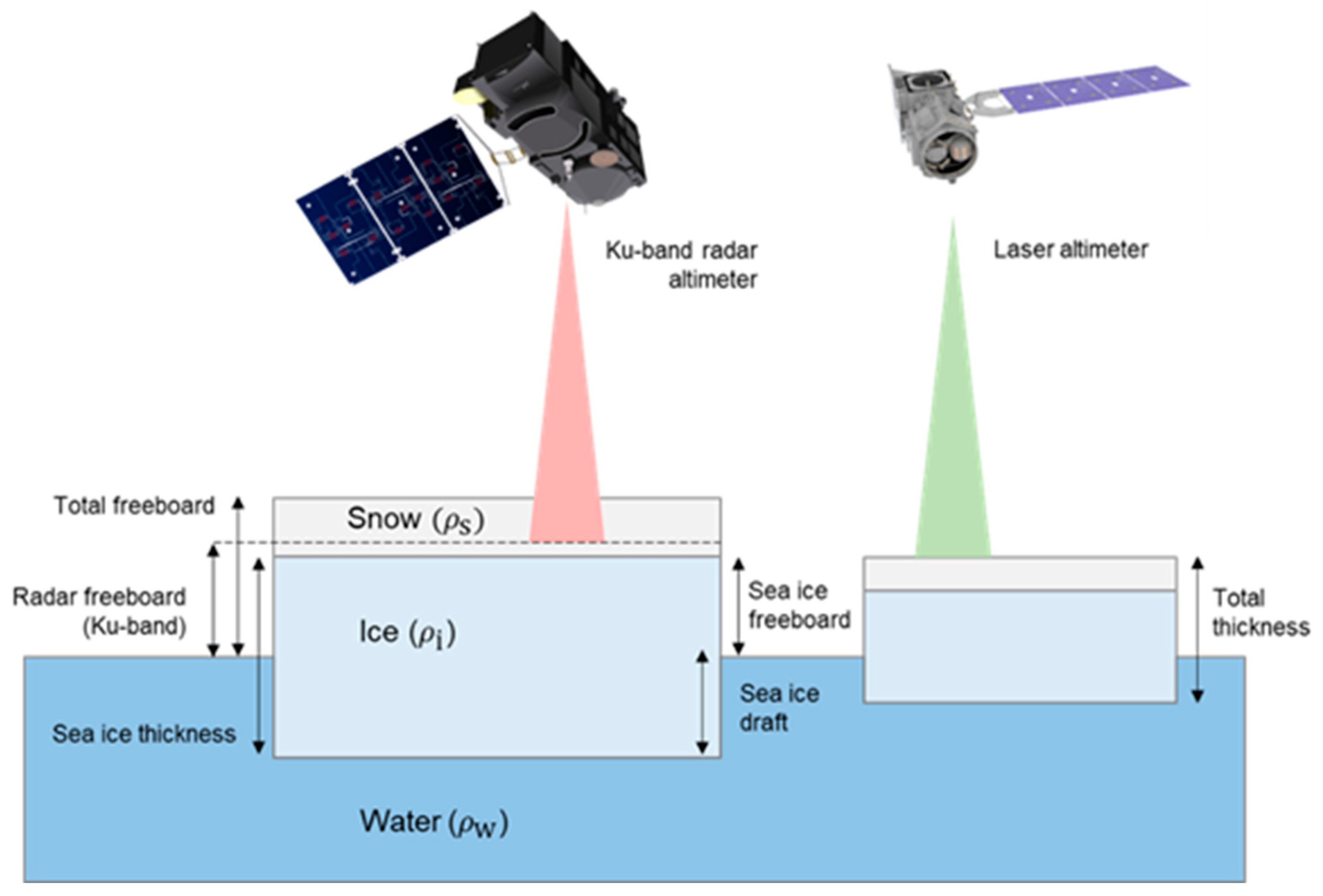
Such a classification can also support the development of operational processing, with more complex algorithms used for more complex sites. Following this convention, four classes have been defined: Complexity Level 0 (CL0), Complexity Level 1 (CL1), Complexity Level 2 (CL2), and Complexity Level 3 (CL3), from the ‘simplest’ case to the ‘most complex’. It is important to note that for sites where the river and the satellite track are collinear, the complexity level can change from CL0 to CL1, or CL2 or CL3, depending on the hydrological properties of the inland water body and the increasing distance between the actual satellite measurement and the reference in situ station. This classification is used to classify the supersite FRMs. In identifying opportunity sites, given the other limits and for the sake of simplicity, we only consider CL0 sites.
Table 1 summarises the parameters used in site classification, including the characteristics of each class and the associated FRM measurement model. As presented in the last row, St3TART has established at least one representative supersite belonging to each class.
These classes make no statement about the quality of the site, or its value for calibration and validation. For a site to be identified as an ‘FRM’, it must be of high quality and provide reliable comparison results for the satellite sensor. The uncertainty associated with a comparison over a CL3 site could, in principle, be smaller than that over a CL1 site, but the equation to calculate it will be longer. The classification is used to describe the complexity of the site. So that Sentinel-3 is validated over a wide range of conditions, it is important to establish supersites of all classes.

4.2. Sea Ice

4.2.1. Existing In Situ Measurements for Sea Ice

Establishing FRM quality measurements of sea ice is challenging. Due to the limited accessibility and logistics, there are few reference observations in the polar areas, and even fewer that provide the full suite of observations required to fully validate the satellite observations. The Cal/Val experiments currently conducted over sea ice for satellite altimetry validation include permanent solutions (upward-looking-sonar (ULS) moored to the bottom of the ocean [35,36,37,50]), semi-permanent solutions (ice mass balance buoys [38,39,51,52] or acoustic buoys [53] anchored to a single floe, which drift along with the ice pack), or campaign observations (airborne, shipborne, or ground-based [40,54,55,56]). Permanent and semi-permanent observations often have high temporal sampling, whereas the spatial sampling is limited to point measurements. For airborne or shipborne campaigns, it is often the opposite case, where spatial sampling is high, but the campaigns are infrequent. Due to limited accessibility and a persistent ice cover in the central Arctic, it is impossible to cover the full Arctic sea ice pack during a yearly cycle. Hence, there will be an overrepresentation of sea ice conditions in more accessible areas (Skourup et al., in prep [40]), resulting in satellite observations only being validated for some conditions (e.g., most airborne flights occur in the Western Arctic along the Canadian and Greenlandic coast, as opposed to the Siberian side). There is a dramatic lack of measurements in Antarctica year-round and of the Arctic summer sea ice.
Observations collected during campaigns depend on the set-up and suite of instruments available: some airborne campaigns collect estimates of radar freeboard, total freeboard (ice + snow freeboard), and snow depth, while others collect observations of total freeboard and total thickness (snow + ice thickness), or other combinations [40,54,57,58].
Although the FRM quantity is a measurement of ice freeboard or sea ice thickness, FRM measurements should also include auxiliary snow depth measurements, and other parameters, more difficult to measure, are also necessary, such as the density of the ice, and to a lesser extent, the density of the snow.

4.2.2. Field Campaigns and Conclusions for Sea Ice

The St3TART project organised two field campaigns:
  • The ESA St3TART 2022 spring campaign in Baffin Bay using new and tested sensors and methods with a fixed winged aircraft, drone, and an autonomous drifting buoy.
  • The Drone Experiment for Sea Ice Retrieval (DESIR) 2022 summer campaign in the central Arctic (Amundsen and Nansen Basin) onboard the ship “Le Commandant Charcot” to test drone deployments from a moving platform, coincident with real-time sea ice thickness measurements obtained using an electromagnetic sensor (the SIMS) mounted on the stern of the ship.
These campaigns provided the opportunity to test and demonstrate new sensors and techniques, including lidar-equipped drones and miniature snow radar additions to autonomous drifting ice thickness (Ice-T) buoys, and demonstrated the challenges associated with conducting field campaigns in the Arctic environment. Where the new sensors and techniques provide the testbed for future FRM for Sentinel-3 Cal/Val on local scales, the airborne observations act as a baseline, as these measurements have already been used for satellite altimetry Cal/Val for the past couple of decades, and link the local scales to regional scales. The airborne team overflew two Sentinel-3A satellite tracks and one Sentinel-3B satellite track, where the Sentinel-3B track was the same track under which the Ice-T buoy was deployed.
The campaigns have demonstrated the capability to use a lidar- and camera-equipped drone system in Arctic conditions with temperatures as low as −13 °C on both land and ship [59]. The total freeboard at the interface between sea ice and water was computed for the data collected by the lidar altimeter, together with surface classification using the camera to take pictures of the observed surface. The campaigns further demonstrated the use of miniature radars to estimate snow depth with an accuracy of the order of a couple of cm from an autonomous drifting Ice-T buoy. Finally, the campaigns used a variety of sensors and platforms for the validation of Sentinel-3 over sea ice, i.e., where the airborne measurements provide regional information of sea ice and total freeboard and surface classification, the Ice-T buoy has the capability to provide ice thickness and snow depth, as well as information on the sea ice drift. The drone provides a link between airborne campaigns by providing seasonal variations on local scales. The Sea Ice Measurement System (SIMS) mounted on the ship turned out to be a great source of evaluation data for the drone measurements, and to have great potential as a future FRM.

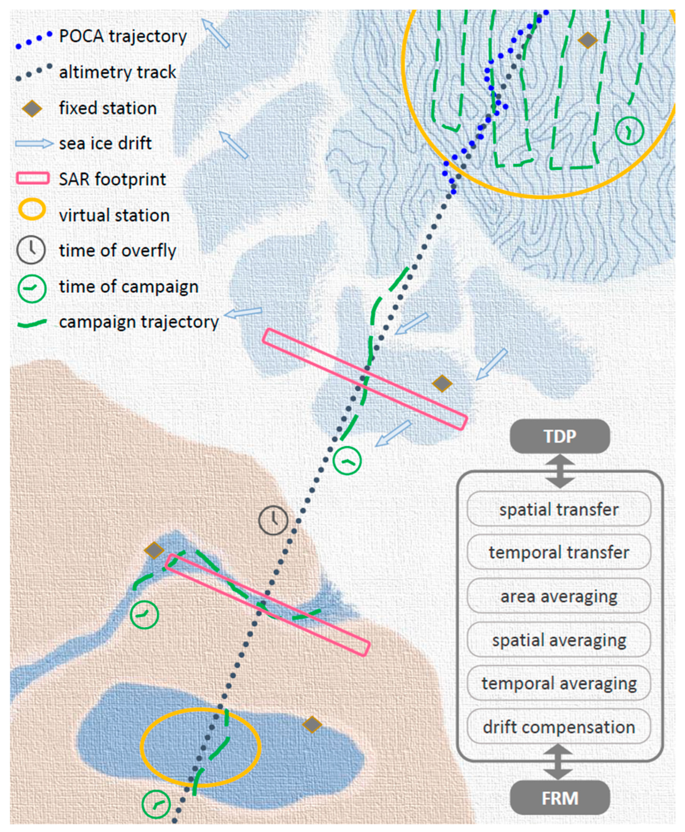
4.2.3. Strategy for Operational FRM Provision over Sea Ice

A suite of FRM measurements for sea-ice-covered regions shall represent seasonal as well as regional coverage, and preferably cover different sea ice types (i.e., first-year and multi-year ice) and different locations in both hemispheres. The selected sites shall further be acquired as far as possible in locations which optimise the number of over-flights by the considered satellite orbit, e.g., for Sentinel-3, below 81.4°N/S, but as close as possible to this high latitude, and preferable at Sentinel-3A/Sentinel-3B crossings. However, options are limited by constraints such as the fact that the long polar nights limit the accessibility for some measurements, such as airborne and helicopter, only allowing such measurements to be obtained from around February to October (exact dates depend on latitude).
In the Arctic, the northern-most coverage of Sentinel-3 leaves a huge uncovered polar gap, which again limits the coverage of multi-year ice to about 10–20% of the total sea-ice-covered regions by Sentinel-3. Thus, it is important to take FRM measurements in the Beaufort Sea, where both ice types are present. Other potential regions are Baffin Bay, the Russian Arctic, or the Fram Strait. Baffin Bay and the Russian Arctic primarily consist of first-year ice, and the Fram Strait is a very dynamic region with high drift speeds, where tying different FRMs and Sentinel-3 measurements together can be very challenging.
Over sea ice, we need to combine different sensors and platforms to provide regional and seasonal coverage. According to the MRTD, each FRM requires uncertainty smaller than 10 cm for sea ice freeboards taken from independent measurements, and 50 cm for sea ice thickness to be useful for Sentinel-3 calibration and validation [6]. As discussed in Section 2.1, FRMs should themselves be intercompared. Operational sensors can be validated through field measurements involving alternative instruments, e.g., using a snow radar when comparing Ku radar measurements with Ka or laser.
Real-time solutions of operational validation data over sea ice are limited to SIMS and drifting buoys, whose data are uplinked by Iridium. Drifting buoys typically provide information about sea ice thickness, temperature profiles, and potential snow depths. Certain post-processing steps might increase the latency time. Other sensors have longer latency times depending on the measurements, e.g., upward-looking moorings that are below the ice need to be physically recovered to obtain access to the data, and this is typically performed once a year by visiting the site with a ship. The post-processing of, e.g., airborne campaign data depends on the number of campaign flights, the number of sensors, the availability and level of processing algorithms, the resources, and the experience of the staff. As a minimum requirement, the FRM shall ideally be provided within a month, and in the worst case scenario, within a year.

4.3. Land Ice

4.3.1. Existing In Situ Measurements for Land Ice

There are two fundamental approaches to provide FRMs over land ice. First, there are survey campaigns that provide profiles of absolute height along tracks that cross the satellite observations. Such absolute survey campaigns can be performed by moving instruments on the ground (e.g., GNSS on a snow vehicle) or from aircraft (crewed or drone, equipped with lidar, radar, or photogrammetry). The second approach is to install a fixed ground station on the ice that takes pseudo-continuous measurements at a frequency greater than the time between satellite overpasses.
In this work, we surveyed existing approaches to identify priorities for FRM sites [60]. To account for small-scale spatial and temporal surface height fluctuations and minimise the impact of small-scale surface roughness variations (e.g., sastrugi) and make the FRM surface elevation time series more robust, the fixed station should consist of several surface-measuring instruments spaced a few metres apart, whose data are checked for outliers and averaged into a time series. A geodetic GNSS receiver should be placed near the surface-measuring instruments to act as an absolute positioning reference.
The in situ station should be installed near where POCA tracks from Sentinel-3 are known to cluster due to surface topography and where the surface topography is stable over time. A reference DSM is needed over the area that covers the possible POCA positions for multiple overpasses along the reference orbit(s). This DSM is generated from a local measurement campaign (by air or on the surface) and should be re-surveyed at a frequency of 1–5 years to document and compensate for any relative topographic changes that are not random. A larger-area DSM allows more POCAs to be compared with the fixed station, helping to reduce noise due to the spatial transfer itself and the radar signal interaction with the variable surface and sub-surface. As a minimum, the DSM should capture all across-track deviations in POCA trajectories from the fixed station, which can vary from a >2 km radius from the fixed station for reasonably flat areas to 10–15 km for areas with complex topography.
As well as such long-term in situ stations, we considered both airborne and in situ observational campaigns as potential FRMs. Existing airborne radar and lidar systems for land ice applications are similar to those used for sea ice. Long-range airborne surveys that operate from an airbase, without requiring any field personnel on the ice, have been more frequent than smaller scale in situ surveys with UAVs.
Airborne surveys over land ice can have multiple purposes:
  • Reference topography (photogrammetry or lidar with complete coverage; can be an FRM)
  • Ice thickness and deep stratigraphy (profiling with low-frequency radar; not relevant for FRM)
  • Snow accumulation and shallow stratigraphy (profiling with high-frequency radar; auxiliary data to an FRM)
  • Ice thickness change and glacier mass balance (repeated surveys of surface elevation; can be part of an FRM)
  • Cal-Val of satellite sensor performance over snow and ice (simulations with comparable instruments)
The two main existing series of airborne campaigns relevant for altimetry Cal/Val in polar regions are NASA’s Operation IceBridge (2009–2019) [40,61] and ESA’s CryoVEx program (active since 2003 in various forms), including coordinated in situ fieldwork on (mainly) Arctic ice caps, the Greenland Ice Sheet and Arctic sea ice (e.g., [62,63]). Both airborne programs have had dual lidar/radar systems onboard, which have facilitated detailed studies of signal penetration, snow depth, and surface mass balance in addition to altimetry validations.
In situ surveys of surface elevation are conducted with kinematic GNSS, with the antenna mounted on a snow vehicle/sledge, or by UAVs using photogrammetry or lidar. Surface GNSS surveys can be targeted on DSM generation via grid-line profiling or on repeats of satellite altimetry ground tracks, e.g., where POCA tracks tend to cluster along topographic ridges such as ice divides [64]. There has been extensive development of surveying techniques to obtain DSM via Structure from Motion (SfM) analysis of UAV optical images in recent years. Motivated by applications in hydrology, there are many studies of snow depth estimation in mountainous areas, based on the subtraction of DSM with and without snow [65,66,67,68]. Applications over land ice in polar regions have typically focused on calving glacier fronts where surface access is otherwise difficult due to crevasses [69].
The use of a UAV lidar system in polar regions is still limited. However, combined with SfM applications, the lidar could allow centimetre-level uncertainties [70], although uncertainties of ~10 cm were obtained by Crocker et al. [71] in Greenland, Svalbard, and over the Southern Ocean (near McMurdo station). Currently, only a small number of UAV lidar observations of ice topography in polar regions have been made.
Established infrastructure sites and observational/logistical transects are attractive for FRM development as they are regularly visited and generally have secured maintenance through respective national polar programs. If sufficient competence and capacity exist, additional Cal/Val activities can be carried out at a relatively low cost compared to establishments in new areas. On the Greenland ice sheet, the PROMICE/GC-NET network of Automatic Weather Stations (AWSs) is unique [72], whereas on the Antarctic Ice Sheet, the IGE GlacioClim network [73,74] between the coastal and inland research stations in Adèlie/Wilkes land stands out for having multiple AWSs in different ice sheet environments. For glaciers and ice caps, it is natural to focus FRM development on the high-latitude polar ice caps where the Sentinel-3 track spacing is dense and where the additional validation aspects of seasonal surface melting and higher surface slopes can be readily assessed. The Austfonna Ice Cap on Svalbard and the Devon Ice Cap in Arctic Canada stand out for their vast sizes and annual field activities through monitoring programs for surface mass balance. These two sites also have a Cal/Val legacy from past CryoVEx campaigns with coordinated airborne (ASIRAS radar, and ALS lidar) and ground-based (kinematic GNSS and radar) surveys, see, e.g., [64,75,76].

4.3.2. Strategy for Operational FRM Provision over Land Ice

To assess land ice elevation changes, we need to assume that the bedrock surface underneath the ice is stable or that its uplift (or subsidence) can be corrected from nearby GNSS observations on ice-free areas or by glacial loading models (e.g., [77]). We also need a stable reference point for the upper surface which can be the true surface of the snow (or ice), or a sub-surface horizon represented by a physical transition in material structure or density. Surface firn and fresh snow layers move with the ice flow, either uniformly by basal sliding (tens to hundreds of metres per year) or more slowly (a few metres per year) from internal deformation in cases where the bed is frozen to the ground. Over time, snow can compact, new snow can accumulate, and snow and firn may erode due to wind and be deposited in new places. In milder climates, snow melts down and sometimes exposes firn or ice at the surface in summer.
All of this means that the surface is changing dynamically, and so there is no simple reference surface for ground-based validation measurements. Surface elevation changes are also difficult to assess due to a lack of stable reference elevations or ground control points to monitor the change against. Regions with strong snow drift also have a particularly complex structure with depositional features at various scales from smaller sastrugi to massive dunes. These formations evolve and migrate with time and align in various ways with the dominant wind direction. The drifting snow provides a very dynamic surface, with spatial scales of decametres that vary in hours, and sometimes minutes. Any in situ measurement needs to average over sufficient spatial and temporal scales to minimise the effect of the drifting snow structures. It also needs to be updated regularly enough to account for the other slower-process changes such as firn compaction and ice motion.
The only way to deal with short-term surface variability is by an FRM from a fixed station installed near Sentinel-3 POCA locations. A geodetic GNSS receiver is needed to act as an absolute positioning reference. The GNSS would be fixed at the ice surface, but then move downslope with the ice. The antenna’s ellipsoidal height is directly measured by the GNSS, whereas its height above the real surface continuously changes with snow accumulation and erosion. GNSS positions would be retrieved using the precise-point-positioning (PPP) technique since GNSS base stations are typically too far away. The relative height of the antenna above the surface would be retrieved using laser scanning or ultrasonic rangers commonly used in existing monitoring programs. More recent work has also investigated the direct retrieval of snow height from GNSS reflections [78].
To account for small-scale spatial and temporal surface height fluctuations and surface roughness variations (e.g., sastrugi), as well as making the FRM surface elevation time series more robust, the fixed station should ideally consist of several surface-measuring instruments spaced a few metres apart, whose data are cross-compared and averaged into a time series. This will provide an averaged local reference elevation over approximately a 5 × 5 m2 area. Annual field visits will, in most cases, be needed to maintain the instruments, as well as to survey and re-evaluate the reference DSM needed for the spatial transfer between the fixed station and the altimetry observation along POCA trajectories.
Observational FRM campaigns beyond the fixed stations should be aimed at the direct validation of multiple Sentinel-3 tracks over a given period (e.g., one Sentinel-3 orbit cycle) when the surface can be assumed to be stable. If the location of POCA tracks can be precisely predicted, or the survey carried out shortly after a satellite overpass, then the navigational flexibility of a snow vehicle makes it possible to follow an undulating POCA track exactly on the ground for direct absolute validation. This can be an efficient way to achieve many comparison points for individual tracks without any need for interpolation.

4.3.3. Towards Metrological Uncertainty for Land Ice Products

An initial uncertainty assessment was performed, identifying and quantifying the key sources of uncertainty in the measurements. This assessment considered the error correlation structures (i.e., systematic and random effects) between different observation stations in the same region and temporarily between measurements at different times. Uncertainties in FRM data from fixed stations will relate to the GNSS, the sonic or laser rangers, and the spatial transfer performed with the DSM. The Cal/Val approach will also need to assess uncertainty in the POCA location and in the interpretation of the waveform, e.g., using electromagnetic models [79]. The PPP method for GNSS measurements avoids the need for a base station and the first-order ionospheric delay is removed through the combination of dual-frequency GNSS measurements. The GNSS satellite orbit and clock error corrections are derived from a network of global reference stations and can be directly delivered by geostationary satellites, but it is preferable to use more precise post-processed products that become available with a delay of a few weeks. Typically, a vertical uncertainty within 10 cm can be achieved depending on the quality of corrections.
The uncertainty of the sonic ranger measurements is related to the spatial variability of surface elevation. For a surface RMS height of typically 7–10 cm, with N = 10 point observations (with ultrasonic gauges or accumulation stakes), the uncertainty would be 2.5 cm (25–35% of the RMSE). For higher surface roughness, more sensors would be needed to achieve similar uncertainty. To reduce the uncertainty associated with the spatial variability in elevation, laser scanning of the FRM site would be a great added value [80]. Including the uncertainty (~10 cm) associated with the acquisition of the DSM, the combined standard uncertainty of a fixed station FRM is expected to be in the range of 20–30 cm.

5. Discussion and Roadmap

In this section we draw conclusions from a review of approaches and the preliminary prototype activities in order to identify where follow up work is needed and how the operational provision of FRM data can be realised.

5.1. Inland Waters

Based on the MPC requirements to meet the MRD (Sentinel-3 Mission Requirements Document) objectives, the recommendations from the CCVS (Copernicus Cal/Val Solution) project, additional discussion with the EEA (European Environment Agency), and following the outcomes of the TD-1 FRM Protocols and Procedure for Sentinel-3 STM Inland Water Products [48], we have defined the following strategy:
  • Establish Cal/Val supersites, where advanced in situ instrumentation is installed on a set of carefully selected sites to ensure the operationality of the FRM production, to serve as a reference in terms of FRM quality, and to allow the analysis, exploration, and better understanding of Sentinel-3 measurements in different configurations of inland waters. A set of eight Cal/Val supersites (Canal du Midi, Garonne River, Po River, Tiber River, Maroni River, Issykkul Lake, Rhine River on both French and German sides, and the Neckar River) have already been identified, equipped, and analysed, and the conclusion for each site [48] has demonstrated the validity of the approach. These sites will continue to be operated and we encourage the establishment of further supersites following the same principles.
  • Make use of opportunity sites from existing in situ networks from different countries to increase the number and variety of comparisons that can be made against Sentinel-3 to establish statistical estimates of performance over inland waters. A non-exhaustive list of public networks that can be used as opportunity sites for the evaluation of the Sentinel-3 performances over inland waters has been identified in [48]. We encourage work to determine the uncertainty associated with these sites so that they can move towards FRM status.
  • Process the data and establish uncertainties of supersites considering the complexity of the sites, as defined by complexity-level classifications. Establishing consistent approaches to processing ensures efficiency of operation. The FRM comparison strategy should include sites from all complexity classes.
  • Ensure rigorous uncertainty analysis, supported by a metrological approach to derive the uncertainty tree diagram, allowing the computation of uncertainty for each class of the complexity-level classification.
  • Extend the approaches established over the lake Cal/Val supersite at Issykkul Lake to other well-maintained lake and reservoir sites.

5.2. Sea Ice

The work described in Section 4.2 has identified state-of-the-art measurements that could be considered to be of FRM quality and has allowed us to establish a consistent FRM framework for such measurements, with an analysis of their maturity level. Considering the dramatic lack of FRM quality measurements for sea ice thickness and snow depth, we recommend two types of action in support of future Sentinel-3 operational provision: (1) the reinforcement of demonstrated methodologies and continuation of long time series and (2) the development of new low-cost approaches.
Concerning (1), we recommend reinforcing the deployment and exploitation of existing upward-looking sonar moorings below the ice through collaborations with oceanographic institutes. It is highly important to secure the maintenance of the existing ice profiling moorings, in particular the Beaufort Gyre Exploration Project [81]. It is also important to extend the network by adding upward-looking sonars to new ocean moorings at key locations, i.e., below 81.4°N, and preferably below Sentinel-3A/Sentinel-3B crossing-points. We further recommend the scientific use of sea ice thickness measurements from icebreakers using SIMS (possibly adding a snow radar) to increase the spatial and temporal coverage. Finally, we recommend continuing recurrent airborne measurements in spring with lidar (or an electromagnetic induction device, such as the Geonics EM31) in combination with a snow radar in the western Arctic to tie regional studies to those of a larger scale. The airborne campaigns shall prioritise under-flights of dedicated Sentinel-3 tracks and over-flights of ice profiling moorings to fully exploit the radar freeboard to draft conversion.
Concerning (2), we recommend deploying several Ice-T IMB buoys which include a snow radar. The deployment site should preferably be in the Beaufort Gyre with deployment in summer, which would allow the buoy to provide measurements through the full season. We further recommend the use of drones equipped with both snow radar and lidar, which have been proven for Arctic conditions as described in Section 4.2.2. Drones will become an essential means of measurement, particularly in hard-to-reach areas, offering an intermediate level of coverage between in situ and airborne systems, and they can be deployed from small Arctic communities, polar stations, or icebreakers, enabling a significant increase in spatial and temporal coverage at a limited cost. To ensure operational capabilities from drone measurements, they would need to be deployed systematically on each expedition, so that their performance can be assessed against other measurements.
In general, particular attention should be paid to measuring the snow depth, which is still very poorly known, and the variable associated with the largest uncertainty in the radar freeboard to sea ice thickness conversion, where it is used both to calculate the snow loading and to calculate the radar propagation delay through the snow layer. Operational measurements of snow depth should be part of a future observing system. We therefore need to ensure the availability of airborne snow radars and support the development of small radars that can be carried by drones, SIMS, and buoys. Without these data, we will not be able to validate the sea ice thickness measurements made by Sentinel-3 and other altimeters, or the snow depth measurements to be made by the future CRISTAL (Copernicus Polar Ice and Snow Topography Altimeter) [82] and CIMR (Copernicus Imaging Microwave Radiometer) [83] missions.
The transition to operational FRM provision requires upstream planning of the post-processing and distribution chains. Indeed, this step is often underestimated and results in considerable delays in the production of FRMs. These delays, which can exceed one year, have an impact on the validation of satellite data. Finally, we underline the fact that validation data of the ice pack are currently extremely rare, and even almost non-existent in Antarctica and during polar summers. Thus, it is necessary to support, gather, process, and distribute acquired data or on-going time series, whether or not they meet all of the criteria to be qualified as FRMs.

5.3. Land Ice

In Section 4.3.2, we outlined a strategy for a fixed station FRM over land ice. This type of combined station with GNSS and sonic rangers [78] is rare in the polar regions and would require annual visits for maintenance. These visits would also be necessary to survey and revaluate the reference DSM that is needed to connect the station with the possible positions of POCA for multiple passes along the reference orbit. To facilitate regular maintenance, these stations should be located near permanent scientific bases or along the logistical supply routes to these bases; see Table A2 and Table A3 (more details in [84]).
The key observations that are required for land ice FRM are as follows:
  • Surface elevation of repeated ground tracks or grids that cover multiple Sentinel-3 ground tracks;
  • Surface elevation time series for seasonal evolution and long-term trends on Sentinel-3 footprint scale;
  • Snow/firn properties (stratigraphy, density, temperature), for relation with volume scattering effects on surface elevation estimates from Ku-band.
The validation data should be collected from sites that are representative of the larger-scale monitoring of glacier and ice sheet mass balance with Sentinel-3 altimetry, in particular ice sheet interiors (low-slope, cold conditions), ice sheet margins (medium slopes, seasonal climate), and polar ice caps or icefields (higher slopes, strong seasonality, widespread melting).
Obtaining continuous FRMs on land ice with fixed stations should be complemented with airborne or in situ survey campaigns along tracks that overlap the satellite observations, as discussed in Section 4.3. Such campaigns can be carried out in a cost-efficient way in combination with FRM station servicing or established in situ monitoring, giving opportunity for further ground transects with kinematic GNSS/GPR or larger-scale UAV surveys. Due to the remoteness and resource-intensive logistics, potential airborne FRM campaigns in Antarctica should be coordinated with other air-based projects as an add-on or side activity, for example, through the SCAR initiative RINGS [85].
In summary, we have the following recommendations for in situ campaigns:
  • Annual or biannual campaigns of 1–2 weeks in the Arctic (Greenland and/or Arctic ice caps) and Antarctica (coastal region) in conjunction with FRM station servicing or established in situ monitoring programmes.
  • Snow vehicle surveys with kinematic GNSS along targeted Sentinel-3 tracks within periods of one month time separation.
  • Auxiliary data should be collected on snow properties (stratigraphy/layers, grain size, density, and temperature) from GPR, probing, snow pits, or shallow cores.
  • Surveys should consider Sentinel-3 processing outputs from different relocation and retracking methods.
  • Surveys should ideally cover a range of surface conditions (smooth, rough, sastrugi, etc.) and slopes.
And, similarly, the recommendations for airborne campaigns are as follows:
  • Airborne campaigns every 2–3 years in the Arctic and every 3–5 years in Antarctica, balancing benefits and costs.
  • Flights from one or more airports in Greenland, Svalbard, or Arctic Canada (station airstrips in Antarctica).
  • Primarily grid-based surveys with lidar and preferably a radar altimeter (e.g., ASIRAS) and optical camera.
  • Survey duration of a few days per 2–5 target areas, of 2–3 weeks in total, including weather days.
  • Coverage of POCA variations for a few selected tracks within a period of one month time separation in each target area.
  • Surveys should cover a range of surface conditions (smooth, rough, sastrugi, etc.) and slopes.
  • One summer campaign over melt-affected areas in the Arctic for contrasting with main reference campaigns in late winter/spring.
  • Coordination with sea ice campaigns and in situ land ice surveys, if possible.

6. Conclusions

The St3TART project aimed to define a roadmap for the operational provision of FRMs for the validation of Sentinel-3 STM Land Thematic Products, based on the definition and consolidation of methods and protocols and identifying the most relevant and cost-effective methods to be maintained, supported, or implemented. This work, performed by different thematic experts for the three surfaces, inland waters, sea ice, and land ice, enabled the identification of the FRM constraints that are unique to each surface. The seasonality, the dynamics of physical variables, and the geographical and climatological constraints are very different; therefore we developed three different FRM strategies and roadmaps as presented here and further detailed in available project reports [48,60,84,86,87,88].
Efficient data distribution is a common need for all three surfaces: all FRM data can be distributed through a unique and centralised system, gathering the different stakeholders around a single platform. Another commonality between surfaces is the methodology used to evaluate uncertainties: we have outlined the “5-step metrological approach”, which was followed to define and quantify the different sources of uncertainties and their impact on the final measurement. There are also some similarities in the sensors used for the three surfaces: GNSS solutions remain the standard for absolute positioning, and drones equipped with lidar have been identified as a promising technique for further development and implementation as a source of FRMs.
Another common conclusion is the importance of auxiliary observational networks, and not only relying on “FRM supersites”. For land ice and sea ice, there are very few relevant measurements available, and so it is essential to consider all of them. For inland waters, it has been demonstrated that opportunity sites are very complementary to FRM supersites.
Finally, it is essential to coordinate FRM efforts with other agencies, such as the EEA, and other projects to mutualise and optimise the campaign and operation costs.

Author Contributions

Conceptualisation: P.F., N.P., E.D.S., M.E.H., J.-C.P., H.S. and G.M.; methodology, validation, formal analysis, investigation, and field work: inland waters: J.-C.P., N.P., V.F. (Valentin Fouqueau), F.B., R.F. (Roger Fjørtoft), A.T., S.C., M.J.T., N.S., N.T., J.R., M.C. (Mathilde Cancet), R.F. (Ramiro Ferrari) and O.A.; sea ice: H.S., S.F., R.M.F.H. and F.V.; land ice: G.M., V.F. (Vincent Favier), J.A., G.P. and E.L.M.; metrology approach: E.R.W. and S.B.; FRM Data Hub development: E.M.; writing—original draft preparation: E.R.W., J.-C.P., H.S., S.F., G.M., V.F. (Vincent Favier), E.D.S., N.P. and S.B.; writing—review and editing: all authors; project administration: E.D.S., P.F. and F.C.; funding acquisition: P.F. All authors have read and agreed to the published version of the manuscript.

Funding

This project was funded by ESA-ESRIN and Copernicus (contract no. 4000135181/21/I-DT). E Woolliams and S. Behnia were additionally funded in the frame of the Instrument Data Quality Evaluation and Assessment Service—Quality Assurance for Earth Observation (IDEAS-QA4EO) contract—funded by ESA-ESRIN (no. 4000128960/19/I-NS).

Data Availability Statement

All data processed during the St3TART project are available through the FRM Data Hub (https://frm-datahub.noveltis.fr/ (Accessed on 3 October 2023).

Acknowledgments

V. Favier and E. Le Meur acknowledge the support of IPEV (program GLACIOCLIM—SAMBA) in defining the roadmap.

Conflicts of Interest

The authors declare no conflict of interest.

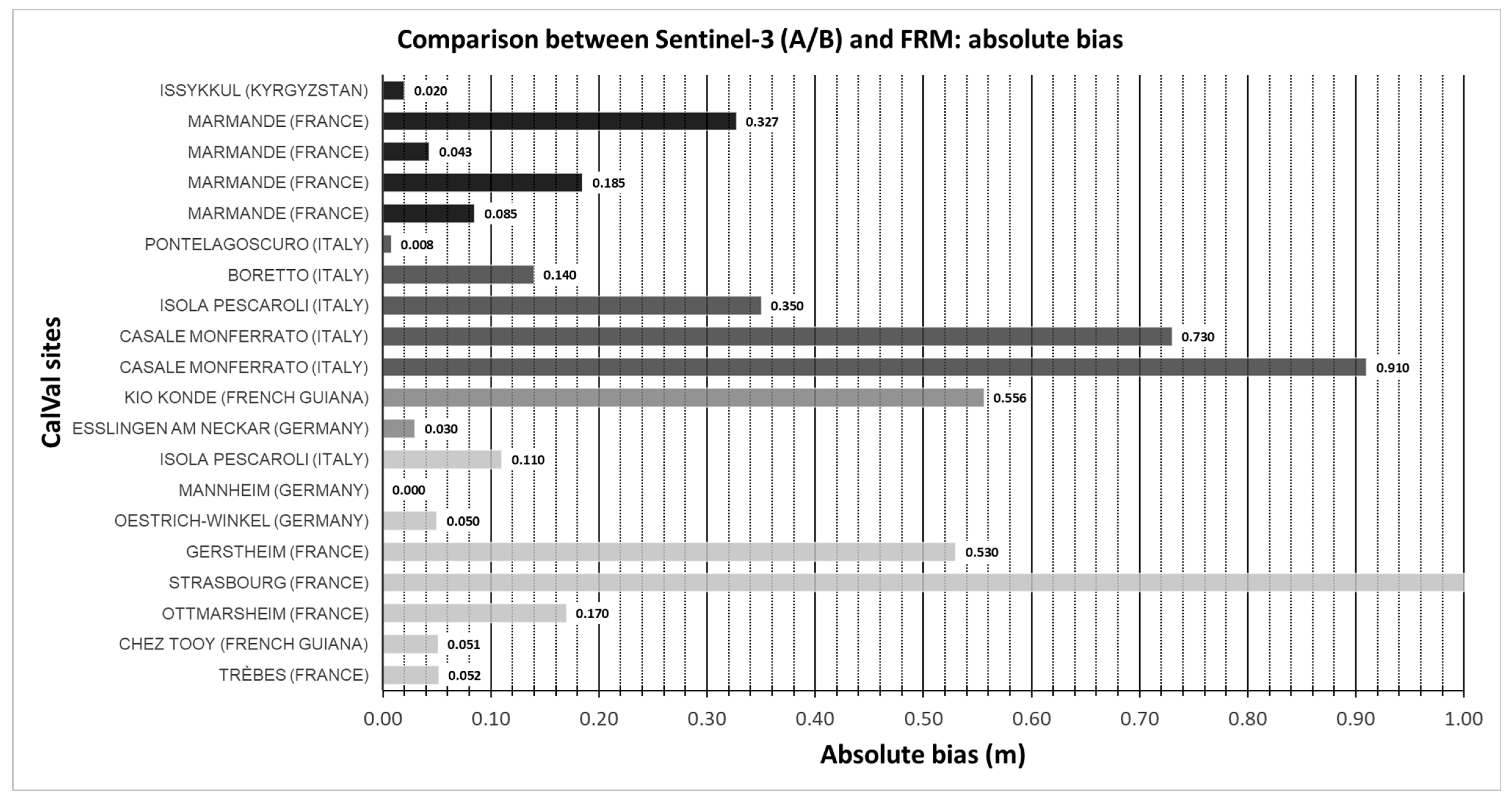
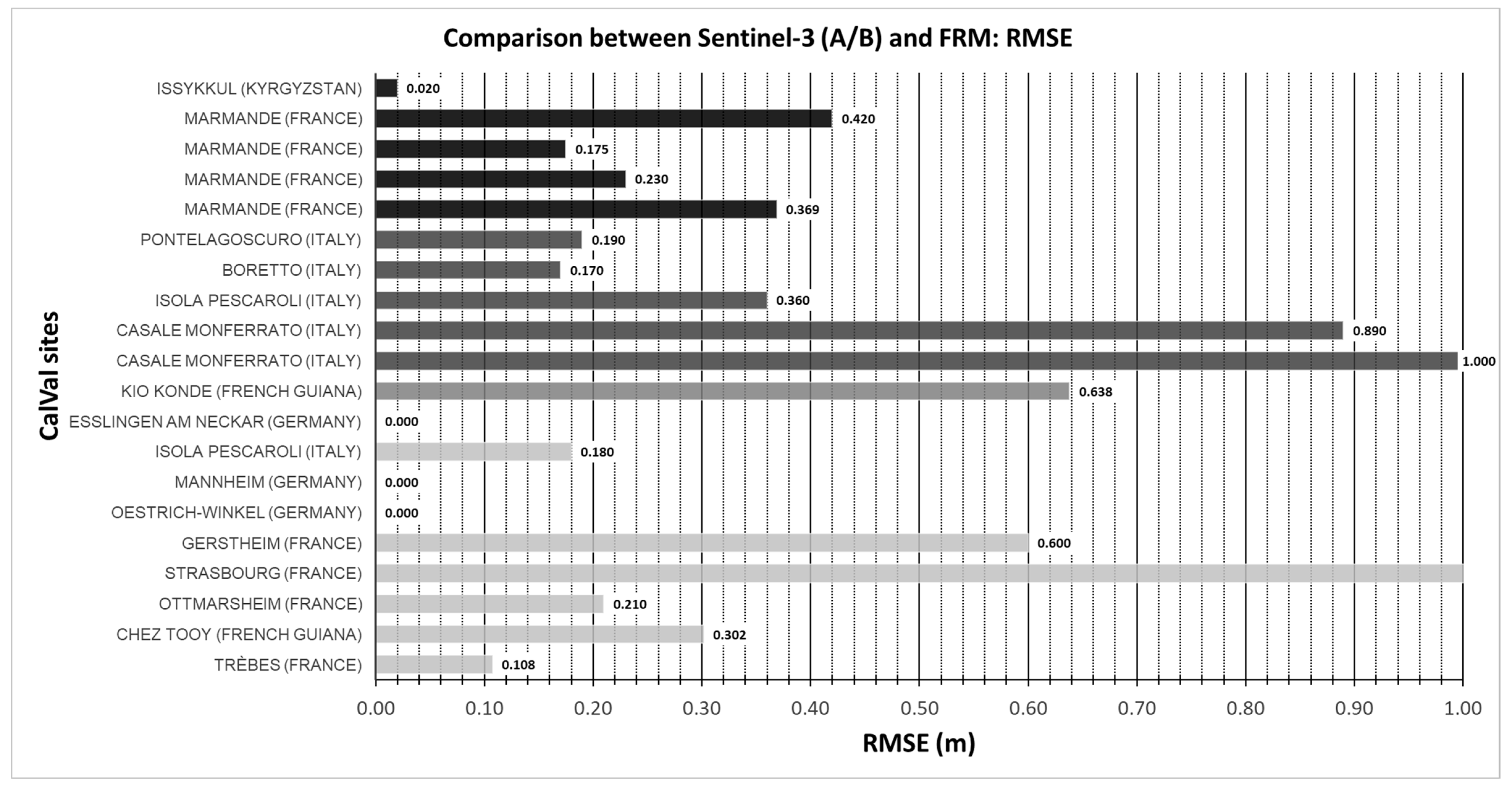
Appendix A. Comparison between Sentinel-3 Data and FRM for Inland Waters

Taking into account the complexity level of each site and associated equations, FRMs were calculated for each Sentinel-3 track over the micro-stations. These FRMs were compared to the Sentinel-3 height measurement. The results obtained over supersites are summarised in Figure A1 and Figure A2, respectively, in terms of RMSE and absolute bias.
Figure A1. RMSE obtained on each site when comparing Sentinel-3 L2 WSE to FRM for each site. Each colour corresponds to a complexity level: light grey for CL0, grey for CL1, dark grey for CL2, and black for CL3.
Remotesensing 15 04826 g0a1
Figure A2. Absolute bias obtained on each site when comparing Sentinel-3 L2 WSE to FRM for each site. Each colour corresponds to a complexity level: light grey for CL0, grey for CL1, dark grey for CL2, and black for CL3.
Remotesensing 15 04826 g0a2
Based on these results and on the overall study of all supersites, the table below describes each supersite and the associated recommendation for the roadmap.
Table A1. Description of each supersite and its associated recommendation.
RiverSiteStation NameSatelliteComplexity LevelRecommendation
Canal du MidiTrèbes (France)trèbes_1S3A0To be maintained
MaroniChez Tooy (French Guiana)chez_tooy_1S3A0To be maintained
Rhine RiverOttmarsheim (France)ottmarsheim_1, chalampé_1S3A0To be maintained
Rhine RiverStrasbourg (France)strasbourg_1S3B0Micro-station must be moved on the other arm of the Rhine River
Rhine RiverGerstheim (France)gerstheim_1S3A0To be maintained
Neckar RiverOestrich-Winkel (Germany)oestrich-winkel_1S3A0To be maintained
Neckar RiverMannheim (Germany)mannheim_2S3A0To be maintained
Po RiverIsola Pescaroli (Italy)isola-pescaroli_1S3B0To be maintained
Neckar RiverEsslingen am Neckar (Germany)esslingen-am-neckar_1S3A1To be maintained
Maroni RiverKio Konde (French Guiana)kio-konde_1S3A1To be changed to Complexity Level 2
Po RiverCasale Monferrato (Italy)casale-monferrato_1S3A2Micro-station must be moved upstream
Po RiverCasale Monferrato (Italy)casale-monferrato_1S3B2Micro-station must be moved upstream
Po RiverIsola Pescaroli (Italy)isola-pescaroli_1S3A2To be changed to Complexity Level 3
Po RiverBoretto (Italy)boretto_1S3A2To be maintained
Po RiverPontelagoscuro (Italy)pontelagoscuro_1S3A2To be maintained
Garonne RiverMarmande (France)marmande_1, marmande_2, le-mas-d-agenais_1S3A3To be maintained
Issykkul LakeIssykkul (Kyrgyzstan)CyclopéeS3A3To be maintained

Appendix B

The tables below list the permanent inland scientific bases and the routes of the logistical traverses supplying these bases, identified during the project as being possible positions to install the FRM stations on.
Table A2. Selected infrastructure sites operated by ESA member states and suitable for S3 land ice FRM development.
RegionSiteLocationInstitute/StationYears of DataInstruments *Surface TypeSlopeS3 Dist.ServiceArea Surveys
AntarcticaCap Prud-homme
66.7°S
139.8°E
0–500 m asl.
IGE, IPEV/GlacioClim2005->Three sites with AWS, SR, GNSSIce sheet margin, snowLowA few kmAnnual, summerAnnual
SvalbardAustfonna Ice Cap79.7°N
22.2°E
200 m asl.
NPI, U. Oslo2004->AWS, SR, GNSSIce cap margin, snow/iceLow800 m, S3A/B
crossover
Annua, springAnnual
GreenlandGreenland Ice SheetNetwork around ice sheetPROMICE/GC-NET, GEUS2007->AWS, SR, GNSSIce sheet margin, snow/iceLowVariable for each stationAnnual, summer
Canadian ArcticDevon Ice Cap75.3°N
82.2°W
1800 m asl.
U. Alberta, Nat. Env. Canada1960->AWS, SRIce cap summit, snowMediumAt S3A nadirAnnual, springAnnual
AntarcticaDome C
75.1°S
123.3°E
3200 m asl.
IGE, IPEV/GlacioClim2005->One site with AWS, SR Ice sheet plateau, snowFlatAt S3A nadirAnnual, summerOccas.
AntarcticaEkström Ice Shelf70.6°S
8.3°W
20 m asl.
Neumayer Station1992->AWS, SR, GNSSIce shelf, snowFlat5 km from S3A nadirCont.Occas.
GreenlandFlade Isblink
Ice Cap
81.5°N
16.6°W
700 m asl.
Station Nord,
Aarhus U.
2006NoIce cap margin, snow/iceLowS3 polar limit on ice cap
* AWS = Automatic Weather Station, SR = sonic ranger.
Table A3. Selected observational and/or logistical ground transects by ESA member states with potential for future S3 FRM use.
RegionSiteLocationLengthInstitute Years of DataInstrumentsSurface TypeSlope# of S3 Profiles Freq.
AntarcticaSAMBA transect76.1°S
123.3°E
0–157 km
157 kmIGE, IPEV/GlacioClim2004->AWS, Kin. GNSS, radar, stakesIce sheet 0–2 deg.>5 acrossAnnual, summer
AntarcticaCap Prudhomme—Dome C66.7°S
139.5°E
0.4–3 km
950 kmIGE, IPEV/GlacioClim AWS, radarSnow, sastrugi0–1 deg.>20 across, >5 alongAnnual, summer
SvalbardAustfonna Ice Cap79.7°N
22.2°E
0–800 m
>20 kmNPI, U. Oslo2004->Kin. GNSS, radar, stakesIce cap, snow0–3 deg.5–10 acrossAnnual, spring
Canadian ArcticDevon Ice Cap75.3°N
82.2°W
0–1800 m
>20 kmU. Alberta, Nat. Env. Canada1961->Kin. GNSS, radar, stakesIce cap, snow0–5 deg.5–10 acrossAnnual, spring
AntarcticaNeumayer–Kohnen Station75°S
4°E
0–2.9 km
750 kmAWI Snow, sastrugi0–2 deg.>20 across, >5 alongOcass.
GreenlandEGIG-line70°N
45°W
0.5–3 km
<600 km EGIG *, ESA CryoVEx, and partners1957->Ice drillIce sheet, snow0–3 deg.>20 acrossOcass.
GreenlandK-Transect67°N
48°W
0.5–2 km
140 kmIMAU Univ. Utrecht1990->AWS, stakesIce and firn0–3 deg.>10 acrossAnnual, summer
AntarcticaCoast—Prince Elisabeth
Station
72.0°S
23.2°E
0–1400 m
200 kmInt. Polar Foundation, Belgium stakesSnow, sastrugi0–2 deg.>15 across,
2 along
Annual, summer
AntarcticaCoast—
Troll
Station
72.0°S
2.5°E
0–1300 m
250 kmNPI Snow, sastrugi0–2 deg.>20 across,
2 along
Annual, summer
* EGIG = Expéditions Glaciologiques Internationales au Groenland in English: International Glaciological Expeditions to Greenland.

References

  1. Donlon, C.; Berruti, B.; Buongiorno, A.; Ferreira, M.-H.; Féménias, P.; Frerick, J.; Goryl, P.; Klein, U.; Laur, H.; Mavrocordatos, C.; et al. The Global Monitoring for Environment and Security (GMES) Sentinel-3 mission. Remote Sens. Environ. 2012, 120, 37–57. [Google Scholar] [CrossRef]
  2. Sentinel-3—Overview—Sentinel Online. Available online: https://copernicus.eu/missions/sentinel-3/overview (accessed on 4 August 2023).
  3. Raney, R. The delay/Doppler radar altimeter. IEEE Trans. Geosci. Remote Sens. 1998, 36, 1578–1588. [Google Scholar] [CrossRef]
  4. Wingham, D.; Francis, C.; Baker, S.; Bouzinac, C.; Brockley, D.; Cullen, R.; de Chateau-Thierry, P.; Laxon, S.; Mallow, U.; Mavrocordatos, C.; et al. CryoSat: A mission to determine the fluctuations in Earth’s land and marine ice fields. Adv. Space Res. 2005, 37, 841–871. [Google Scholar] [CrossRef]
  5. Quartly, G.D.; Nencioli, F.; Raynal, M.; Bonnefond, P.; Garcia, P.N.; Garcia-Mondéjar, A.; de la Cruz, A.F.; Crétaux, J.-F.; Taburet, N.; Frery, M.-L.; et al. The Roles of the S3MPC: Monitoring, Validation and Evolution of Sentinel-3 Altimetry Observations. Remote Sens. 2020, 12, 1763. [Google Scholar] [CrossRef]
  6. Donlon, C. Sentinel-3 Mission Requirements Traceability Document (MRTD). 2011. no. 1. Available online: https://sentinel.esa.int/documents/247904/1848151/sentinel-3-mission-requirements-traceability (accessed on 3 October 2023).
  7. Goryl, P.; Donlan, C.; Fox, N. Fiducial Reference Measurements (FRM): What are they? Remote Sens. (under review). No. Special issue on Copernicus Sentinels Missions Calibration Validation, FRM and innovation approaches in satellite-data quality assessment.
  8. QA4EO Home. Available online: https://www.qa4eo.org/ (accessed on 7 June 2023).
  9. SENTINEL3 ST3TART. 2 March 2023. Available online: https://sentinel3-st3tart.noveltis.fr/ (accessed on 4 August 2023).
  10. Mittaz, J.; Merchant, C.J.; Woolliams, E.R. Applying principles of metrology to historical Earth observations from satellites. Metrologia 2019, 56, 032002. [Google Scholar] [CrossRef]
  11. BIPM; IEC; IFCC; ILAC; ISO; IUPAC; IUPAP; OIML. Evaluation of Measurement Data—Guide to the Expression of Uncertainty in Measurement. 2008. Available online: https://www.bipm.org/documents/20126/2071204/JCGM_100_2008_E.pdf (accessed on 3 October 2023).
  12. User Guides—Sentinel-3 Altimetry—Processing Levels—Sentinel Online. Available online: https://sentinels.copernicus.eu/web/sentinel/user-guides/sentinel-3-altimetry/processing-levels (accessed on 4 August 2023).
  13. ESA-Fundamental-Data-Records-for-Atmospheric-Composition-(FDR4ATMOS)-Status-and-Updates. Available online: https://earth.esa.int/eogateway/documents/20142/1484253/ESA-Fundamental-Data-Records-for-Atmospheric-Composition-%28FDR4ATMOS%29-status-and-updates.pdf (accessed on 3 October 2023).
  14. Mertikas, S.P.; Donlon, C.; Féménias, P.; Mavrocordatos, C.; Galanakis, D.; Tripolitsiotis, A.; Frantzis, X.; Tziavos, I.N.; Vergos, G.; Guinle, T. Fifteen Years of Cal/Val Service to Reference Altimetry Missions: Calibration of Satellite Altimetry at the Permanent Facilities in Gavdos and Crete, Greece. Remote Sens. 2018, 10, 1557. [Google Scholar] [CrossRef]
  15. Surface Topography Mission (STM) SRAL/MWR L2 Algorithms Definition, Accuracy and Specification|EUMETSAT. Available online: https://www-cdn.eumetsat.int/files/2020-04/pdf_s3_alt_level_2_adas.pdf (accessed on 8 August 2023).
  16. Wingham, D.J.; Rapley, C.G.; Griffiths, H. New techniques in satellite altimeter tracking systems. In Proceedings of the IGARSS 1986, Zürich, Switzerland, 8–11 September 1986; Volume 86, pp. 1339–1344. [Google Scholar]
  17. Abileah, R.; Scozzari, A.; Vignudelli, S. Envisat RA-2 Individual Echoes: A Unique Dataset for a Better Understanding of Inland Water Altimetry Potentialities. Remote Sens. 2017, 9, 605. [Google Scholar] [CrossRef]
  18. Laxon, S. Sea ice altimeter processing scheme at the EODC. Int. J. Remote Sens. 1994, 15, 915–924. [Google Scholar] [CrossRef]
  19. Drinkwater, M.R.; Kwok, R.; Winebrenner, D.P.; Rignot, E. Multifrequency polarimetric synthetic aperture radar observations of sea ice. J. Geophys. Res. Atmos. 1991, 96, 20679–20698. [Google Scholar] [CrossRef]
  20. Laxon, S.; Peacock, N.; Smith, D. High interannual variability of sea ice thickness in the Arctic region. Nature 2003, 425, 947–950. [Google Scholar] [CrossRef]
  21. Giles, K.A.; Laxon, S.W.; Ridout, A.L. Circumpolar thinning of Arctic sea ice following the 2007 record ice extent minimum. Geophys. Res. Lett. 2008, 35, L22502. [Google Scholar] [CrossRef]
  22. Tilling, R.L.; Ridout, A.; Shepherd, A. Estimating Arctic sea ice thickness and volume using CryoSat-2 radar altimeter data. Adv. Space Res. 2018, 62, 1203–1225. [Google Scholar] [CrossRef]
  23. Laxon, S.W.; Giles, K.A.; Ridout, A.L.; Wingham, D.J.; Willatt, R.; Cullen, R.; Kwok, R.; Schweiger, A.; Zhang, J.; Haas, C.; et al. CryoSat-2 estimates of Arctic sea ice thickness and volume. Geophys. Res. Lett. 2013, 40, 732–737. [Google Scholar] [CrossRef]
  24. Ricker, R.; Hendricks, S.; Helm, V.; Skourup, H.; Davidson, M. Sensitivity of CryoSat-2 Arctic sea-ice freeboard and thickness on radar-waveform interpretation. Cryosphere 2014, 8, 1607–1622. [Google Scholar] [CrossRef]
  25. Birkett, C. Synergistic Remote Sensing of Lake Chad Variability of Basin Inundation. Remote Sens. Environ. 2000, 72, 218–236. [Google Scholar] [CrossRef]
  26. Crétaux, J.-F.; Birkett, C. Lake studies from satellite radar altimetry. Comptes Rendus Geosci. 2006, 338, 1098–1112. [Google Scholar] [CrossRef]
  27. Le Gac, S.; Boy, F.; Blumstein, D.; Lasson, L.; Picot, N. Benefits of the Open-Loop Tracking Command (OLTC): Extending conventional nadir altimetry to inland waters monitoring. Adv. Space Res. 2019, 68, 843–852. [Google Scholar] [CrossRef]
  28. Da Silva, J.S.; Calmant, S.; Seyler, F.; Filho, O.C.R.; Cochonneau, G.; Mansur, W.J. Water levels in the Amazon basin derived from the ERS 2 and ENVISAT radar altimetry missions. Remote Sens. Environ. 2010, 114, 2160–2181. [Google Scholar] [CrossRef]
  29. Kwok, R.; Kacimi, S. Three years of sea ice freeboard, snow depth, and ice thickness of the Weddell Sea from Operation IceBridge and CryoSat-2. Cryosphere 2018, 12, 2789–2801. [Google Scholar] [CrossRef]
  30. Kurtz, N.T.; Farrell, S.L.; Studinger, M.; Galin, N.; Harbeck, J.P.; Lindsay, R.; Onana, V.D.; Panzer, B.; Sonntag, J.G. Sea ice thickness, freeboard, and snow depth products from Operation IceBridge airborne data. Cryosphere 2013, 7, 1035–1056. [Google Scholar] [CrossRef]
  31. King, J.; Skourup, H.; Hvidegaard, S.M.; Rösel, A.; Gerland, S.; Spreen, G.; Polashenski, C.; Helm, V.; Liston, G.E. Comparison of Freeboard Retrieval and Ice Thickness Calculation From ALS, ASIRAS, and CryoSat-2 in the Norwegian Arctic to Field Measurements Made During the N-ICE2015 Expedition. J. Geophys. Res. Oceans 2018, 123, 1123–1141. [Google Scholar] [CrossRef]
  32. Haas, C.; Beckers, J.; King, J.; Silis, A.; Stroeve, J.; Wilkinson, J.; Notenboom, B.; Schweiger, A.; Hendricks, S. Ice and Snow Thickness Variability and Change in the High Arctic Ocean Observed by In Situ Measurements. Geophys. Res. Lett. 2017, 44, 10,462–10,469. [Google Scholar] [CrossRef]
  33. Kwok, R.; Rothrock, D.A. Decline in Arctic sea ice thickness from submarine and ICESat records: 1958–2008. Geophys. Res. Lett. 2009, 36, L15501. [Google Scholar] [CrossRef]
  34. Belter, H.J.; Krumpen, T.; Hendricks, S.; Hoelemann, J.; Janout, M.A.; Ricker, R.; Haas, C. Satellite-based sea ice thickness changes in the Laptev Sea from 2002 to 2017: Comparison to mooring observations. Cryosphere 2020, 14, 2189–2203. [Google Scholar] [CrossRef]
  35. Spreen, G.; de Steur, L.; Divine, D.; Gerland, S.; Hansen, E.; Kwok, R. Arctic Sea Ice Volume Export Through Fram Strait From 1992 to 2014. J. Geophys. Res. Oceans 2020, 125, e2019JC016039. [Google Scholar] [CrossRef]
  36. Khvorostovsky, K.; Hendricks, S.; Rinne, E. Surface Properties Linked to Retrieval Uncertainty of Satellite Sea-Ice Thickness with Upward-Looking Sonar Measurements. Remote Sens. 2020, 12, 3094. [Google Scholar] [CrossRef]
  37. Hansen, E.; Gerland, S.; Granskog, M.A.; Pavlova, O.; Renner, A.H.H.; Haapala, J.; Løyning, T.B.; Tschudi, M. Thinning of Arctic sea ice observed in Fram Strait: 1990–2011. J. Geophys. Res. Oceans 2013, 118, 5202–5221. [Google Scholar] [CrossRef]
  38. Richter-Menge, J.A.; Perovich, D.K.; Elder, B.C.; Claffey, K.; Rigor, I.; Ortmeyer, M. Ice mass-balance buoys: A tool for measuring and attributing changes in the thickness of the Arctic sea-ice cover. Ann. Glaciol. 2006, 44, 205–210. [Google Scholar] [CrossRef]
  39. Liao, Z.; Cheng, B.; Zhao, J.; Vihma, T.; Jackson, K.; Yang, Q.; Yang, Y.; Zhang, L.; Li, Z.; Qiu, Y.; et al. Snow depth and ice thickness derived from SIMBA ice mass balance buoy data using an automated algorithm. Int. J. Digit. Earth 2018, 12, 962–979. [Google Scholar] [CrossRef]
  40. MacGregor, J.A.; Boisvert, L.N.; Medley, B.; Petty, A.A.; Harbeck, J.P.; Bell, R.E.; Blair, J.B.; Blanchard-Wrigglesworth, E.; Buckley, E.M.; Christoffersen, M.S.; et al. The Scientific Legacy of NASA’s Operation IceBridge. Rev. Geophys. 2021, 59, e2020RG000712. [Google Scholar] [CrossRef]
  41. Helm, V.; Humbert, A.; Miller, H. Elevation and elevation change of Greenland and Antarctica derived from CryoSat-2. Cryosphere 2014, 8, 1539–1559. [Google Scholar] [CrossRef]
  42. Howat, I.M.; Porter, C.; Smith, B.E.; Noh, M.-J.; Morin, P. The Reference Elevation Model of Antarctica. Cryosphere 2019, 13, 665–674. [Google Scholar] [CrossRef]
  43. McMillan, M.; Muir, A.; Shepherd, A.; Escolà, R.; Roca, M.; Aublanc, J.; Thibaut, P.; Restano, M.; Ambrozio, A.; Benveniste, J. Sentinel-3 Delay-Doppler altimetry over Antarctica. Cryosphere 2019, 13, 709–722. [Google Scholar] [CrossRef]
  44. Smith, B.; Fricker, H.A.; Gardner, A.S.; Medley, B.; Nilsson, J.; Paolo, F.S.; Holschuh, N.; Adusumilli, S.; Brunt, K.; Csatho, B.; et al. Pervasive ice sheet mass loss reflects competing ocean and atmosphere processes. Science 2020, 368, 1239–1242. [Google Scholar] [CrossRef] [PubMed]
  45. Chupin, C.; Ballu, V.; Testut, L.; Tranchant, Y.-T.; Calzas, M.; Poirier, E.; Coulombier, T.; Laurain, O.; Bonnefond, P.; Team FOAM Project. Mapping Sea Surface Height Using New Concepts of Kinematic GNSS Instruments. Remote Sens. 2020, 12, 2656. [Google Scholar] [CrossRef]
  46. Boy, F.; Cretaux, J.-F.; Boussaroque, M.; Tison, C. Improving Sentinel-3 SAR Mode Processing Over Lake Using Numerical Simulations. IEEE Trans. Geosci. Remote Sens. 2021, 60, 1–18. [Google Scholar] [CrossRef]
  47. Crétaux, J.-F.; Bergé-Nguyen, M.; Calmant, S.; Jamangulova, N.; Satylkanov, R.; Lyard, F.; Perosanz, F.; Verron, J.; Montazem, A.S.; Le Guilcher, G.; et al. Absolute Calibration or Validation of the Altimeters on the Sentinel-3A and the Jason-3 over Lake Issykkul (Kyrgyzstan). Remote Sens. 2018, 10, 1679. [Google Scholar] [CrossRef]
  48. Poisson, J.-C.; The St3TART Hydro Group. TD-1 FRM Protocols and Procedure for S3 STM Inland Water Products’. Available online: https://sentinel3-st3tart.noveltis.fr/wp-content/uploads/2023/06/NOV-FE-0899-NT-042_TD-1-Inland-FRM-Standard-procedures-and-protocols_V3.2.pdf (accessed on 3 October 2023).
  49. Wilkinson, M.D.; Dumontier, M.; Aalbersberg, I.J.; Appleton, G.; Axton, M.; Baak, A.; Blomberg, N.; Boiten, J.W.; da Silva Santos, L.B.; Bourne, P.E.; et al. The FAIR Guiding Principles for scientific data management and stewardship. Sci. Data 2016, 3, 160018. [Google Scholar] [CrossRef]
  50. Belter, H.J.; Janout, M.A.; Hölemann, J.A.; Krumpen, T. Daily mean sea ice draft from moored upward-looking Acoustic Doppler Current Profilers (ADCPs) in the Laptev Sea from 2003 to 2016. Pangaea 2020. [Google Scholar] [CrossRef]
  51. Sato, K.; Inoue, J. Comparison of Arctic sea ice thickness and snow depth estimates from CFSR with in situ observations. Clim. Dyn. 2017, 50, 289–301. [Google Scholar] [CrossRef]
  52. Perovich, D.K.; Richter-Menge, J.A.; Polashenski, C. Observing and Understanding Climate Change: Monitoring the Mass Balance, Motion, and Thickness of Arctic Sea Ice. Available online: http://imb-crrel-dartmouth.org/results/ (accessed on 3 October 2023).
  53. Nicolaus, M.; Riemann-Campe, K.; Bliss, A.; Hutchings, J.K.; Granskog, M.A.; Haas, C.; Hoppmann, M.; Kanzow, T.; Krishfield, R.A.; Lei, R. Drift Trajectory of the Site LM of the Distributed Network of MOSAiC 2019/2020; Alfred Wegener Institute, Helmholtz Centre for Polar and Marine Research: Bremerhaven, Germany, 2021. [Google Scholar] [CrossRef]
  54. Skourup, H.; Olesen, A.V.; Sandberg Sørensen, L.; Simonsen, S.; Hvidegaard, S.M.; Hansen, N.; Olesen, A.F.; Coccia, A.; Macedo, K.; Helm, V. ESA CryoVEx/KAREN and EU ICE-ARC 2017. Final Rep. 2017. Available online: https://earth.esa.int/eogateway/documents/20142/1526226/CryoVEx2017-final-report.pdf (accessed on 3 October 2023).
  55. Willatt, R.C.; Giles, K.A.; Laxon, S.W.; Stone-Drake, L.; Worby, A.P. Field Investigations of Ku-Band Radar Penetration Into Snow Cover on Antarctic Sea Ice. IEEE Trans. Geosci. Remote Sens. 2009, 48, 365–372. [Google Scholar] [CrossRef]
  56. Renner, A.H.H.; Gerland, S.; Haas, C.; Spreen, G.; Beckers, J.F.; Hansen, E.; Nicolaus, M.; Goodwin, H. Evidence of Arctic sea ice thinning from direct observations. Geophys. Res. Lett. 2014, 41, 5029–5036. [Google Scholar] [CrossRef]
  57. Herber, A.; Becker, S.; Belter, H.J.; Brauchle, J.; Ehrlich, A.; Klingebiel, M.; Krumpen, T.; Lüpkes, C.; Mech, M.; Moser, M.; et al. MOSAiC Expedition: Airborne Surveys with Research Aircraft POLAR 5 and POLAR 6 in 2020. Ber. Zur Polar-Und Meeresforsch. Rep. Polar Mar. Res. 2021, 754, 1–99. [Google Scholar] [CrossRef]
  58. Krumpen, T.; Gerdes, R.; Haas, C.; Hendricks, S.; Herber, A.; Selyuzhenok, V.; Smedsrud, L.; Spreen, G. Recent summer sea ice thickness surveys in Fram Strait and associated ice volume fluxes. Cryosphere 2016, 10, 523–534. [Google Scholar] [CrossRef]
  59. Skourup, H.; Fleury, S.; Poisson, J.-C.; Fouqueau, V.; Vivier, F.; Lourenço, A. TD-13-2 Final Campaign Report for Sea Ice. Available online: https://sentinel3-st3tart.noveltis.fr/wp-content/uploads/2023/06/NOV-FE-0899-NT-102_TD-13-2_-V2.1-SeaIceFinalCampaignReport.pdf (accessed on 3 October 2023).
  60. Moholdt, G.; Favier, V.; Aublanc, J. TD-3 FRM Protocols and Procedure for S3 STM Land Ice Products. Available online: https://sentinel3-st3tart.noveltis.fr/wp-content/uploads/2023/06/NOV-FE-0899-NT-044-V4.1-TD-3-Land-Ice-FRM-Standard-procedures-and-protocols.pdf (accessed on 3 October 2023).
  61. Hofton, M.A.; Luthcke, S.B.; Blair, J.B. Estimation of ICESat intercampaign elevation biases from comparison of lidar data in East Antarctica. Geophys. Res. Lett. 2013, 40, 5698–5703. [Google Scholar] [CrossRef]
  62. Hawley, R.L.; Morris, E.M.; Cullen, R.; Nixdorf, U.; Shepherd, A.P.; Wingham, D.J. ASIRAS airborne radar resolves internal annual layers in the dry-snow zone of Greenland. Geophys. Res. Lett. 2006, 33, L04502. [Google Scholar] [CrossRef]
  63. Sørensen, L.S.; Simonsen, S.B.; Langley, K.; Gray, L.; Helm, V.; Nilsson, J.; Stenseng, L.; Skourup, H.; Forsberg, R.; Davidson, M.W.J. Validation of CryoSat-2 SARIn Data over Austfonna Ice Cap Using Airborne Laser Scanner Measurements. Remote Sens. 2018, 10, 1354. [Google Scholar] [CrossRef]
  64. Morris, A.; Moholdt, G.; Gray, L.; Schuler, T.V.; Eiken, T. CryoSat-2 interferometric mode calibration and validation: A case study from the Austfonna ice cap, Svalbard. Remote Sens. Environ. 2021, 269, 112805. [Google Scholar] [CrossRef]
  65. Revuelto, J.; Alonso-Gonzalez, E.; Vidaller-Gayan, I.; Lacroix, E.; Izagirre, E.; Rodríguez-López, G.; López-Moreno, J.I. Intercomparison of UAV platforms for mapping snow depth distribution in complex alpine terrain. Cold Reg. Sci. Technol. 2021, 190, 103344. [Google Scholar] [CrossRef]
  66. Adams, M.S.; Bühler, Y.; Fromm, R. Multitemporal Accuracy and Precision Assessment of Unmanned Aerial System Photogrammetry for Slope-Scale Snow Depth Maps in Alpine Terrain. Pure Appl. Geophys. 2017, 175, 3303–3324. [Google Scholar] [CrossRef]
  67. Avanzi, F.; Bianchi, A.; Cina, A.; De Michele, C.; Maschio, P.; Pagliari, D.; Passoni, D.; Pinto, L.; Piras, M.; Rossi, L. Centimetric Accuracy in Snow Depth Using Unmanned Aerial System Photogrammetry and a MultiStation. Remote Sens. 2018, 10, 765. [Google Scholar] [CrossRef]
  68. Bühler, Y.; Adams, M.S.; Bösch, R.; Stoffel, A. Mapping snow depth in alpine terrain with unmanned aerial systems (UAS): Potential and limitations. Cryosphere 2016, 10, 1075–1088. [Google Scholar] [CrossRef]
  69. Köhler, A.; Pętlicki, M.; Lefeuvre, P.-M.; Buscaino, G.; Nuth, C.; Weidle, C. Contribution of calving to frontal ablation quantified from seismic and hydroacoustic observations calibrated with lidar volume measurements. Cryosphere 2019, 13, 3117–3137. [Google Scholar] [CrossRef]
  70. Li, T.; Zhang, B.; Xiao, W.; Cheng, X.; Li, Z.; Zhao, J. UAV-Based Photogrammetry and LiDAR for the Characterization of Ice Morphology Evolution. IEEE J. Sel. Top. Appl. Earth Obs. Remote Sens. 2020, 13, 4188–4199. [Google Scholar] [CrossRef]
  71. Crocker, R.I.; Maslanik, J.A.; Adler, J.J.; Palo, S.E.; Herzfeld, U.C.; Emery, W.J. A Sensor Package for Ice Surface Observations Using Small Unmanned Aircraft Systems. IEEE Trans. Geosci. Remote Sens. 2011, 50, 1033–1047. [Google Scholar] [CrossRef]
  72. Fausto, R.S.; van As, D.; Mankoff, K.D.; Vandecrux, B.; Citterio, M.; Ahlstrøm, A.P.; Andersen, S.B.; Colgan, W.; Karlsson, N.B.; Kjeldsen, K.K.; et al. Programme for Monitoring of the Greenland Ice Sheet (PROMICE) automatic weather station data. Earth Syst. Sci. Data 2021, 13, 3819–3845. [Google Scholar] [CrossRef]
  73. Favier, V.; Agosta, C.; Genthon, C.; Arnaud, L.; Trouvillez, A.; Gallée, H. Modeling the mass and surface heat budgets in a coastal blue ice area of Adelie Land, Antarctica. J. Geophys. Res. Earth Surf. 2011, 116, F03017. [Google Scholar] [CrossRef]
  74. Agosta, C.; Favier, V.; Genthon, C.; Gallée, H.; Krinner, G.; Lenaerts, J.T.M.; Broeke, M.R.v.D. A 40-year accumulation dataset for Adelie Land, Antarctica and its application for model validation. Clim. Dyn. 2011, 38, 75–86. [Google Scholar] [CrossRef]
  75. Hawley, R.L.; Brandt, O.; Dunse, T.; Hagen, J.O.; Helm, V.; Kohler, J.; Langley, K.; Malnes, E.; Høgda, K.-A. Using airborne Ku-band altimeter waveforms to investigate winter accumulation and glacier facies on Austfonna, Svalbard. J. Glaciol. 2013, 59, 893–899. [Google Scholar] [CrossRef]
  76. Gray, L.; Burgess, D.; Copland, L.; Demuth, M.N.; Dunse, T.; Langley, K.; Schuler, T.V. CryoSat-2 delivers monthly and inter-annual surface elevation change for Arctic ice caps. Cryosphere 2015, 9, 1895–1913. [Google Scholar] [CrossRef]
  77. Schumacher, M.; A King, M.; Rougier, J.; Sha, Z.; A Khan, S.; Bamber, J.L. A new global GPS data set for testing and improving modelled GIA uplift rates. Geophys. J. Int. 2018, 214, 2164–2176. [Google Scholar] [CrossRef]
  78. Dahl-Jensen, T.S.; Citterio, M.; Jakobsen, J.; Ahlstrøm, A.P.; Larson, K.M.; Khan, S.A. Snow Depth Measurements by GNSS-IR at an Automatic Weather Station, NUK-K. Remote Sens. 2022, 14, 2563. [Google Scholar] [CrossRef]
  79. Larue, F.; Picard, G.; Aublanc, J.; Arnaud, L.; Robledano-Perez, A.; LE Meur, E.; Favier, V.; Jourdain, B.; Savarino, J.; Thibaut, P. Radar altimeter waveform simulations in Antarctica with the Snow Microwave Radiative Transfer Model (SMRT). Remote Sens. Environ. 2021, 263, 112534. [Google Scholar] [CrossRef]
  80. Picard, G.; Arnaud, L.; Panel, J.-M.; Morin, S. Design of a scanning laser meter for monitoring the spatio-temporal evolution of snow depth and its application in the Alps and in Antarctica. Cryosphere 2016, 10, 1495–1511. [Google Scholar] [CrossRef]
  81. Beaufort Gyre Exploration Project. Available online: https://www2.whoi.edu/site/beaufortgyre/ (accessed on 7 June 2023).
  82. Kern, M.; Cullen, R.; Berruti, B.; Bouffard, J.; Casal, T.; Drinkwater, M.R.; Gabriele, A.; Lecuyot, A.; Ludwig, M.; Midthassel, R.; et al. The Copernicus Polar Ice and Snow Topography Altimeter (CRISTAL) high-priority candidate mission. Cryosphere 2020, 14, 2235–2251. [Google Scholar] [CrossRef]
  83. Vanin, F.; Laberinti, P.; Donlon, C.; Fiorelli, B.; Barat, I.; Sole, M.P.; Palladino, M.; Eggers, P.; Rudolph, T.; Galeazzi, C. Copernicus Imaging Microwave Radiometer (CIMR): System Aspects and Technological Challenges. In Proceedings of the IGARSS 2020—2020 IEEE International Geoscience and Remote Sensing Symposium, Waikoloa, HI, USA, 26 September–2 October 2020; pp. 6535–6538. [Google Scholar] [CrossRef]
  84. Moholdt, G.; Favier, V.; Aublanc, J. TD-6-3—Roadmap for S3 STM Land FRM Operational Provision over Land Ice. Available online: https://sentinel3-st3tart.noveltis.fr/wp-content/uploads/2023/06/NOV-FE-0899-NT-052_TD-6-Land-Ice-Roadmap_V4.1.pdf (accessed on 3 October 2023).
  85. RINGS Ice Sheet Margin. Available online: https://www.scar.org/science/rings/home/ (accessed on 7 June 2023).
  86. Skourup, H.; Woolliams, E.; Fredensborg Hansen, R.M.; Fleury, S.; Behnia, S. TD-2 FRM Protocols and Procedure for S3 STM Sea Ice Products. Available online: https://sentinel3-st3tart.noveltis.fr/wp-content/uploads/2023/06/NOV-FE-0899-NT-043-V4.1-TD-2-Sea-Ice-FRM-Standard-procedures-and-protocols.pdf (accessed on 3 October 2023).
  87. Poisson, J.-C.; The St3TART Hydro Group. TD-6-1—Roadmap for S3 STM Land FRM Operational Provision for Inland Waters. Available online: https://sentinel3-st3tart.noveltis.fr/wp-content/uploads/2023/06/NOV-FE-0899-NT-050_TD6-Roadmap-for-Inland-Waters_V4.1.pdf (accessed on 3 October 2023).
  88. Skourup, H.; Fleury, S.; Sea Ice Team. TD-6-2—Roadmap for S3 STM Land FRM Operational Provision for Sea Ice. Available online: https://sentinel3-st3tart.noveltis.fr/wp-content/uploads/2023/06/NOV-FE-0899-NT-051_V4.1_TD-6_Roadmap_SeaIce.pdf (accessed on 3 October 2023).
Figure 1. Sea ice variables and parameters of relevance to the altimetry measurements. Adapted from CPOM.
Remotesensing 15 04826 g001
Figure 2. Schematic drawing of a satellite track going over the different surfaces of interest, from ice sheet (top) to sea ice (middle) and rivers/lakes (bottom). A full description is given in the text. The altimeter track is represented by the dotted black line (with each dot representing a 20 Hz measurement, where the footprint of such measurements is indicated by the magenta rectangles). Over land ice (top part of diagram), the point of closest approach is calculated from the underlying topography (shown as the bright blue dots in that part of the diagram). For each surface, an FRM is likely to combine a fixed station (the grey diamonds) and possibly occasional field campaigns (green dashed lines) to understand variability around the observations, or within a ‘virtual station’ (yellow ovals/circles).
Remotesensing 15 04826 g002
Figure 3. FRM provisioning strategy.
Remotesensing 15 04826 g003
Table 1. Summary of the site classification.
CL0CL1CL2CL3
Characteristics
-
Located under satellite ground track
-
No slope correction from instrument to satellite track
-
No propagation time correction
-
Not necessarily located under satellite ground track
-
No propagation time correction (river not changing rapidly)
-
Slope correction between river height at instrument and satellite track but not dependent on the water height
-
Not necessarily located under satellite ground track
-
Propagation time correction (river changing over travel time from instrument to satellite track)
-
Slope correction but not dependent on the water height
-
Not necessarily located under satellite ground track
-
Propagation time correction
-
Slope correction evolving with the water height
FRM measurement model parametersWater surface height at the in situ sensorWater surface height plus slope correction for river height differencesWater surface height corrected for water propagation time plus slope correction Water surface height corrected for propagation time plus time-dependent slope correction
FRM measurement model h ( t ) h t + Δ h slope h t + Δ t + Δ h slope h t + Δ t + Δ h slope ( t )
Cal/Val sitesTrèbes, Po River (Isola Pescaroli for S3B), Tiber River (Santa Lucia)Grand Canal d’Alsace (French part of the Rhine River)German RhineGaronne River, Po River, Tiber River
Disclaimer/Publisher’s Note: The statements, opinions and data contained in all publications are solely those of the individual author(s) and contributor(s) and not of MDPI and/or the editor(s). MDPI and/or the editor(s) disclaim responsibility for any injury to people or property resulting from any ideas, methods, instructions or products referred to in the content.

