GSDerainNet: A Deep Network Architecture Based on a Gaussian Shannon Filter for Single Image Deraining

Abstract

With the continuous advancement of target detection technology in remote sensing, target detection technology in images captured by drones has performed well. However, object detection in drone imagery is still a challenge under rainy conditions. Rain is a common severe weather condition, and rain streaks often degrade the image quality of sensors. The main issue of rain streaks removal from a single image is to prevent over smoothing (or underclearing) phenomena. Aiming at the above problems, this paper proposes a deep learning (DL)-based rain streaks removal framework called GSDerainNet, which properly formulates the single image rain streaks removal problem; rain streaks removal is aptly described as a Gaussian Shannon (GS) filter-based image decomposition problem. The GS filter is a novel filter proposed by us, which consists of a parameterized Gaussian function and a scaled Shannon function. Two-dimensional GS filters exhibit high stability and effectiveness in dividing an image into low- and high-frequency parts. In our framework, an input image is first decomposed into a low-frequency part and a high-frequency part by using the GS filter. Rain streaks are located in the high-frequency part. We extract and separate the rain features of the high-frequency part through a deep convolutional neural network (CNN). The experimental results obtained on synthetic data and real data show that the proposed method can better suppress the morphological artifacts caused by filtering. Compared with state-of-the-art single image rain streaks removal methods, the proposed method retains finer image object structures while removing rain streaks.

1. Introduction

Computer vision technology endows drones with autonomous perception, analysis and decision-making capabilities, and target detection is one of the key technologies to improve the perception capabilities of drones. The drone image target detection algorithm is effectively applied in practical scenarios such as traffic monitoring, power inspection, crop analysis and disaster rescue. However, under rainy weather conditions, rain streaks often degrade the visual quality of images or videos, resulting in greatly reduced accuracy of object detection [1]. Rain streaks interfere and degrade the performance of computer vision and image processing algorithms. Effective methods for removing rain streaks are needed for a wide range of practical applications, such as drone capture [1], object detection/recognition [2], autonomous driving [3,4] and improving the visibility of humans [5]. Therefore, rain streak removal is an important fundamental problem in image processing and computer vision research.

Methods for removing rain streaks from images are divided into two categories: video-based methods and single-image-based methods. In the last decade, many researchers have devoted their attention to removing the effects of rain streaks on videos and single image quality. We briefly review video-based methods for removing rain streaks. Due to the interframe information that exists in video, it is easier to remove rain streaks in videos [6,7,8,9]. For example, Islam and Paul [6] proposed making a better video by exploiting rain appearance duration, shape, and location to remove rain streaks from a video. Abdel-Hakim [7] exploited the interframe information to put the problem in a convex optimization form and then used low-rank restoration to remove rain and snow from a video. Dou et al. [8] proposed a sparse tensor model based on the main direction of rain streaks to remove video rain streaks. Lee et al. [9] proposed a deep learning (DL)-based recurrent neural network (RNN) architecture to remove rain streaks in videos. These methods are effective for removing rain streaks in videos. However, single image rain removal is more difficult than video rain removal due to the lack of temporal correlation and context information. In this paper, we focus on removing rain streaks from a single image.

Removing rain streaks from a single image is more challenging. The key issue in removing rain streaks from a single image is preventing over (or under) rain removal [10]. Excessive removal of rain streaks can cause the fine structures of objects to be removed. Insufficient rain removal is a small number of rain streaks left in the image. Rain streaks or overly smooth images can degrade the performance of a computer vision system. Some existing single image rain removal methods focus on removing rain streaks by adopting various image priors. For example, the Gaussian mixture model (GMM) [11] and discriminative sparse coding (DSC) [12] techniques have been used to remove rain streaks. These methods are effective in certain scenarios. However, when the rainfall is heavy, these methods do not have sufficiently fine structures to recover the pixels affected by the rainfall, resulting in severely blurred background images. Such prior model-based techniques lack generalization ability and cannot flexibly adapt to rainy images with complex rain shapes and background scenes. A disadvantage of methods [11] is that they often leave rain streaks in the derained results, while methods [12] tend to generate oversmoothed results when dealing with images containing fine structures such as rain streaks. Zheng et al. [13] used multiguided filters for single-image-based rain and snow removal. However, the disadvantage of guided filtering and weighted guided filtering [14] is that they often lead to over-smoothing results when the rain streaks are similar to the image structures, especially the fine structure part [15].

DL-based methods have achieved remarkable results in single image rain streaks removal [16,17,18,19]. Hu et al. [16] proposed the rain-density squeeze-and-excitation residual network (RDSER-NET) to remove rain streaks from a single image. The network proposed by Hu et al. removes rain steaks based on a single density of rain steaks in the training data, which reduces the limitation of multidensity proposals and achieves better results. Yang et al. [17] used contextualized deep networks to jointly detect and remove rain streaks from a single image. To address the motion blur problem of line patterns caused by rain removal methods, Wang et al. [18] used a kernel-guided convolutional neural network (KGCNN) to remove rain streaks from a single image. Rain removal methods based on deep learning generally require a large amount of training data. To handle image rain removal well even with small training datasets, Jang et al. [19] proposed a lightweight deep extraction network (DEN). DL approaches based on neural networks can solve problems in various complex application models, which provides excellent performance for removing rain streaks from a single image.

To cleanly remove rain streaks while preserving a finer structure of the image, in this paper, we propose a rain removal framework based on a Gaussian Shannon (GS) filter and a deep CNN. The deep CNN provides good performance for removing rain streaks from a single image. To further improve the accuracy of rain removal we proposed a new two-dimensional GS filter. The cutoff frequency and transition band length of the GS filter are independently adjusted by the scale parameter of the Shannon function and the window width parameter of the Gaussian function, which is why the filter has good flexibility. The proposed GSDerainNet consists of two steps: rain image filtering and rain streak removal. Our method can cleanly remove rain streaks, preserve the fine structure, and suppress the range of morphological artifacts by adjusting the parameters of the GS filter. The GS filter is used to extract the high-frequency part where rain streaks exist. In the rain streak removal phase, the high-frequency parts extracted by GS filtering are input into a deep CNN model for training and removing rain streaks. Retaining finer structures while removing rain streaks without morphological artifacts is the motivation of this paper.

The rest of this paper is arranged as follows: In Section 2, we summarize related works on single image rain removal. In Section 3, we provide the mathematical expression of the proposed GS filter and discuss the details of GSDerainNet. In Section 4, we conduct experiments with datasets and present the experimental results. In Section 5, we discuss our method. In Section 6, we draw conclusions as to the effectiveness of our method.

2. Related Works

Existing single image rain removal methods vary in their performance in the successful removal of rain streaks. Especially when an object’s structure and orientation are similar to rain streaks, it can be difficult to simultaneously remove rain streaks and preserve the structure. To address this difficult problem, DL techniques have been applied to single image rain removal tasks; this category of methods learns nonlinear mappings from rainy images to rainless images in an end-to-end manner [20,21,22]. Fu et al. [23] and Yang et al. [24] both built deep CNN models with datasets containing various rain density levels, directions and shapes to train learning-based image rain removal models. Fu et al. [25] removed rain from a single image via a deep detail network (DDN). Zhang et al. [26] used a density-aware multistream dense network (DID-MDN) to remove rain from a single image. Wang et al. [27] used a high-quality real rain dataset for spatially attentive single image denoising. Wang et al. [28] proposed a model-driven deep neural network for single image rain removal. The effectiveness of these methods depends heavily on the quality and quantity of the training samples input to and output by the network. The above studies show that a deep CNN can also provide excellent single image rain removal performance.

Dictionary learning methods have been proposed to remove rain streaks from a single image [12,29]. First, the input rain image is decomposed into a base layer and a detail layer with rain streaks, and then sparse coding dictionary learning is used to detect and remove rain streaks in the detail layer. In [12], the authors used discriminative sparse coding to recover clean images from rainy images. Chen et al. [29] used a guided image filter to decompose the input color image into low-frequency and high-frequency parts and then decomposed the high-frequency part into rain and non-rain components through dictionary learning and sparse coding. However, dictionary learning-based frameworks require significant computation time [23]. To obtain a satisfactory CNN model, some researchers have attempted to decompose a given rain image into a low-frequency part and a high-frequency part using different filters, such as guided filters [30,31], Gaussian filters [32,33], and bilateral filters [34,35]. They treated the single image rain removal challenge as an image decomposition problem with two layers: rain streaks and background scenes [36]. Training on the detail layer rather than the image domain can save computational resources and improve the convergence of the CNN [23]. In addition, we fixed the model structure and set different filters to compare the rain removal effect, as shown in Figure 1. Some fine structures in the image are blurred in the results of the guided filter (Figure 1b) and bilateral filter (Figure 1d), and some rain streaks are preserved in the results of the Gaussian filter (Figure 1c). As shown in Figure 1e, the background of the result of the proposed algorithm removing rain streaks is clearer.

Fu et al. [23] proposed a low-pass filter to extract the detail part of the image and train a DerainNet model with a three-layer CNN structure in the detail part to remove rain. Fu et al. [25] proposed a DDN, which uses a guided filter to obtain the detailed part of the image as the input of the residual network (ResNet) and ResNet as the parameter layer to obtain the deeper feature map of the image. Yeh et al. [32] divided a single rainy image into a high-frequency part and a low-frequency part via a Gaussian filter for rain removal. The proposed Gaussian filter is used for preprocessing before the CNN step. Pal et al. [35] proposed a deraining framework for rainy images based on L₀ gradient minimization and bilateral filtering. A disadvantage of the method in [34] is that it tends to produce oversmoothed results when dealing with images possessing complex rain streak features. In the approach presented in [32], the disadvantage is that they usually leave rain streaks in the deraining result. To address the low-frequency errors contained in the recovered structures, Pan et al. [37] proposed a dual convolutional neural network architecture (DualCNN) for low-level vision. DuanCNN includes two parallel branches, Net-S and Net-D, to restore the low-frequency structure and high-frequency details, respectively. Ye et al. [38] proposed a bidirectional disentangled translation network to remove rain streaks from a single image, where each unidirectional network contains two loops of joint rain generation and removal for real and synthetic rain images, respectively. The model in [38] greatly simplifies translation by performing translation on the rain layer instead of the image, since the rain layer space is much simpler than the image space. In an end-to-end learning rain removal framework, the methods [37,38] obtain detail layers by decomposing rainy images to preserve finer structures. The deep CNN provides excellent performance and favorable conditions for removing rain streaks. The model that combines deep CNN and filter decomposition images works well in removing rain streaks from a single image. Therefore, in this paper, we designed a single image rain streaks removal framework called GSDerainNet that combines a GS filter with a deep CNN.

3. Materials and Methods

We present the developed rain removal framework based on the GS filter. As discussed in more detail below, the GS filter is proposed to decompose each image into a low-frequency rainless image information layer and a high-frequency rain feature layer. The rain feature layer is the input into the CNN so that the model can learn the features of rain and remove rain streaks.

3.1. Gaussian Shannon Filter for the Rain Feature Layer

We propose a new low-pass filter called the GS filter, which is defined as

$${\theta }_s^{\sigma }(t)=\mathit{exp}(-\frac{t^2}{2{\sigma }^2})\frac{\mathit{sin}(2\pi t/s)}{\pi t},$$

(1)

where t represents time. σ represents the transition band parameter, which determines the time-domain length of the filter and controls the transition band length of the filter frequency domain. s represents the cutoff scale parameter, which determines the cutoff period or frequency. Although the time axis of the Gaussian window is infinitely long since approximately 99.73% of the energy of the Gaussian function is mainly concentrated in the interval with the mean as the center and three times the standard deviation as the radius, the length of the function filter corresponding to Formula (1) can be t∈[−3σ, 3σ]. Formula (1) is a low-pass filter whose convolution can realize filtering processing. The proposed filter possesses features such that the transition band and cutoff frequency can be independently controlled by two parameters σ and s, respectively, and the cutoff frequency and transition frequency can be controlled independently.

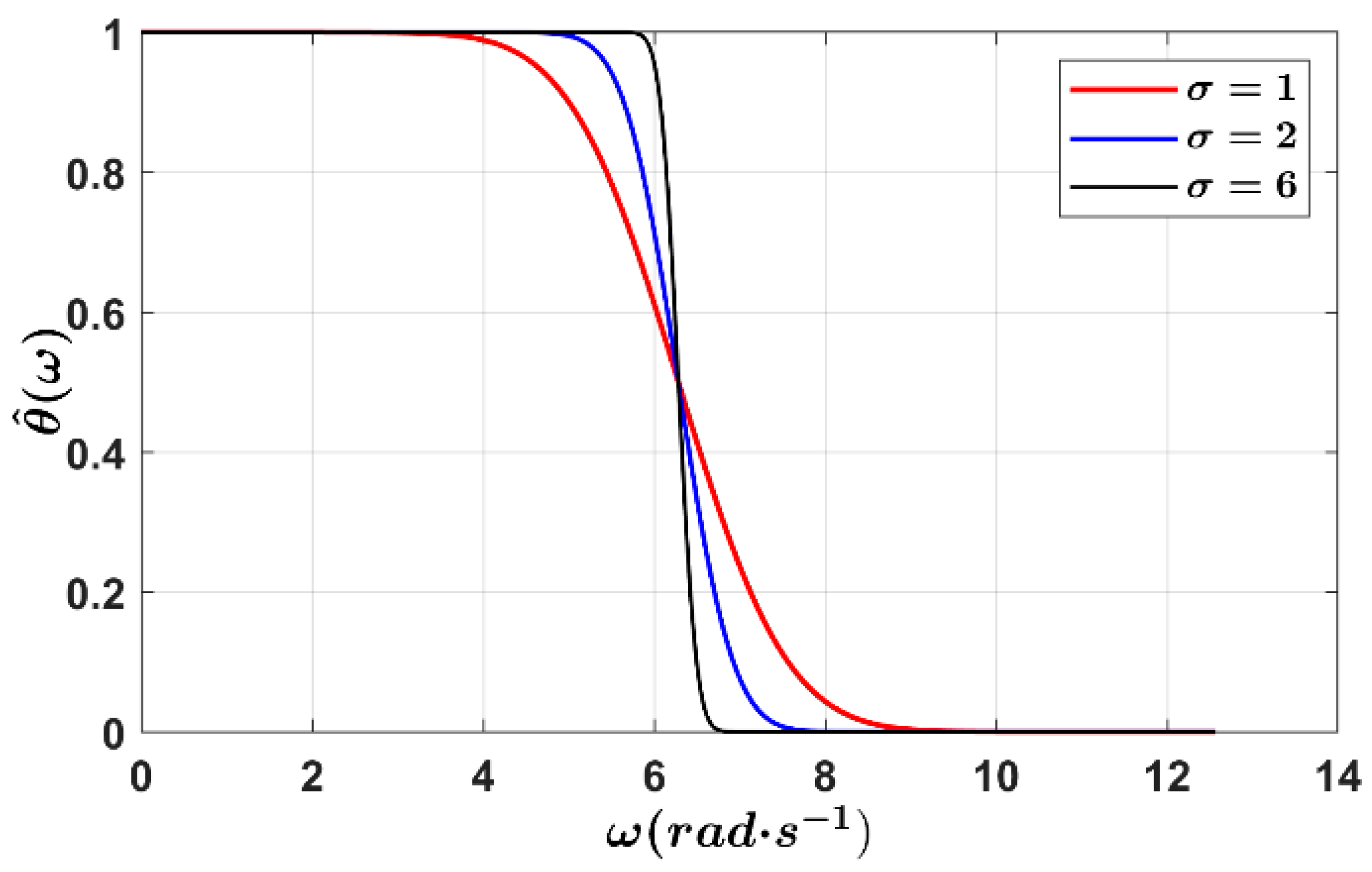
As shown in Figure 2, we analyze the frequency response of the low-pass function filter and perform a Fourier transform on the low-pass filter of Formula (1). The frequency response formula of the GS filter is as follows:

$$\widehat{\theta }\left(\omega \right)=\frac{\mathit{ERF}\left(\frac{\sigma }{\sqrt{2}}\left(\omega +\frac{2\pi }{s}\right)\right)-\mathit{ERF}\left(\frac{\sigma }{\sqrt{2}}\left(\omega -\frac{2\pi }{s}\right)\right)}{2},$$

(2)

where “^” represents the Fourier transform, and ERF(x) represents the error function: $\frac{2}{\sqrt{\pi }}{\int }_0^{x}exp\left(-t^2\right)dt$. The cutoff scale of the function filter is s; that is, the cutoff frequency is 2π/s. For example, when the passband fluctuation is 0.05, the passband edge is approximately a linear function of 1/σ, which is expressed as −1.65/σ + 2π/s; when the stopband fluctuation is 0.05, the stopband edge is approximately a linear function of 1/σ, expressed as 1.65/σ + 2π/s. Therefore, the transition band length is 3.3/σ, which is controlled only by σ. We further demonstrate that the two parameters σ and s of the GS filter affect the transition band and cutoff frequency, respectively, and that these two parameters are independent of each other.

In this paper, we propose a new two-dimensional GS filter to remove rain streaks in images; this filter is defined as Formula (3), which is essentially a Gaussian-modulated scaled Shannon function.

$${\theta }_s^{\sigma }(x,y)=\mathit{exp}(-\frac{x^2+y^2}{2{\sigma }^2})\frac{\mathit{sin}(2\pi \sqrt{x^2+y^2}/s)}{\pi \sqrt{x^2+y^2}},$$

(3)

In the formula, (x, y) represents the coordinates of the two-dimensional function in the spatial domain. σ represents the transition band parameter, which determines the time-domain length of the filter and controls the transition band length of the filter frequency domain; s represents the cutoff scale parameter, which determines the cutoff period or frequency. The frequency response of the two-dimensional GS filter is shown in Figure 3. As shown in Figure 3a, the transition band parameters are fixed, and the cutoff scale parameters are flexibly adjusted, which can also be achieved by a Gaussian filter. However, compared to the two-dimensional Gaussian filter, we add an independent transition band parameter σ. The transition band parameters and cutoff scale parameters of the proposed new filter are independently adjustable.

3.2. Our Network Structure

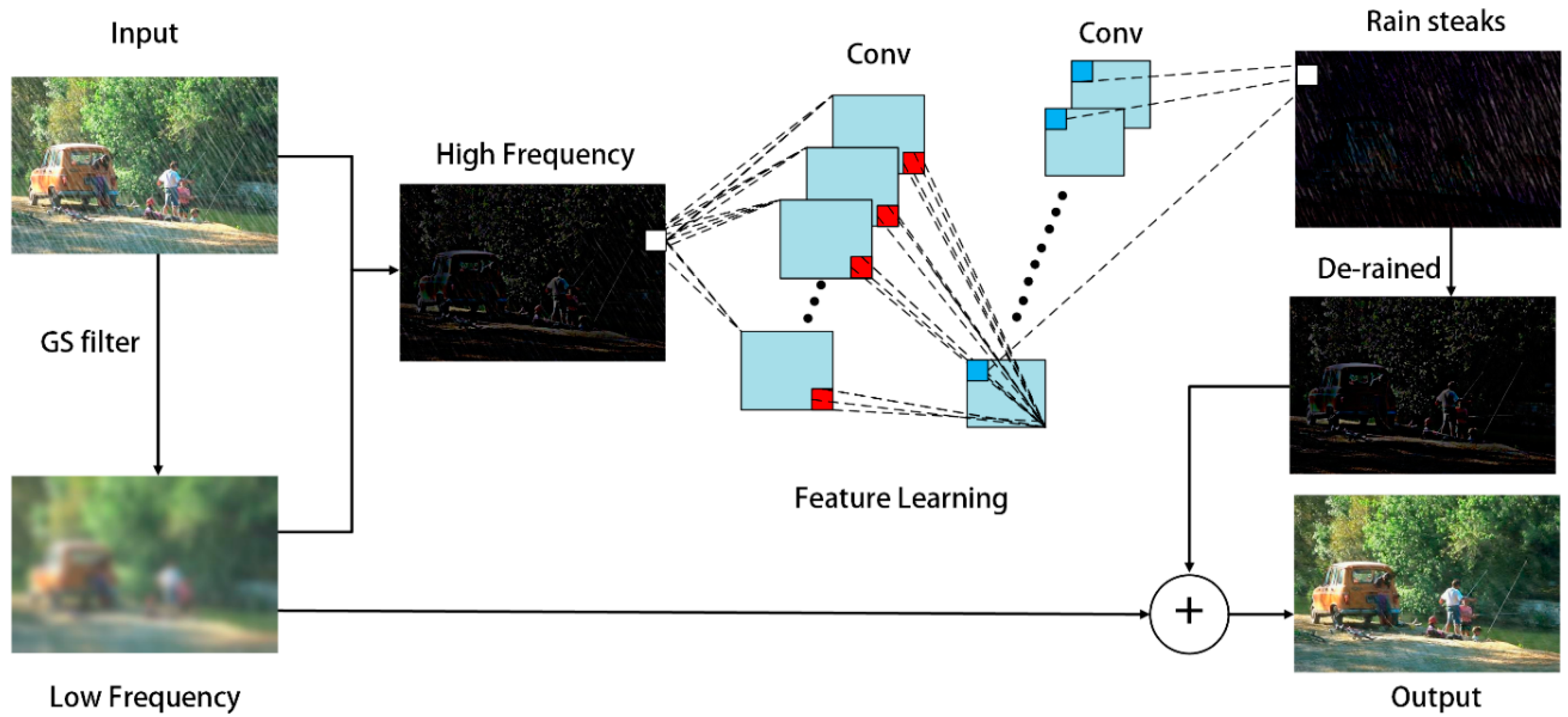
According to Fu et al.’s research [23], it is not necessarily feasible to introduce more complex network structures to obtain satisfactory training results. The rain removal problem is a low-level image task. Introducing more complex deep structures to such image processing problems may cause overfitting. To effectively solve the rain removal problem, we use a GS filter to modify the objective function rather than increasing the depth of the model. We illustrate the proposed model framework in Figure 4. We use a GS filter to decompose the input image into the sum of its rainless layer and rain feature layer, rather than directly feeding the rain image into the model for training.

To train the rain removal model, we denote the input rain image and the corresponding clean image as X and Y, respectively. First, the image is decomposed into the sum of its low-frequency components and high-frequency components by GS filtering, as shown in Formula (4). The low-frequency layer is represented by the “low” layer, and the high-frequency rain feature layer is represented by the “high” layer.

$$X=X_{low}+X_{high},$$

(4)

We use the GS filter to filter the clean map and rain map separately. The difference between the low-frequency parts of the clean image and the rainy image is small, as shown in Figure 5, and the high-frequency results are shown in Figure 6b,d. We count the pixel value changes exhibited by the R, G, and B channels of the high-frequency part of the image before and after filtering. As shown in Figure 6f–j, the pixel values of most areas in the high-frequency detail layer are close to zero. Therefore, we train the CNN model through the high-frequency detail layer, which can simplify the CNN model in terms of learning the mapping relationships. Exploiting the sparsity of high-frequency detail layers is a widely used technique in existing deraining methods [10,38,39,40]. For DL models, training a CNN on the detail layer also follows the process of mapping input patches to output patches, and the mapping range is significantly reduced, so the model training results do not require more computation time and data samples. In addition, to demonstrate the effectiveness of our proposed method, we suppress the artifacts generated by the edges of the filtered image by adjusting the transition band.

As shown in Figure 7, we compare the filtered low-frequency and high-frequency parts of the GS filter at the same cutoff frequency. Adjusting the transition band parameters of the GS filter can effectively control the range of morphological artifacts in the high-frequency part. Combined with the a priori experimental analysis, we choose the optimal transition band parameter σ = 10, which ensures that the rain streak in the low-frequency part is removed cleanly and that the high-frequency part produces fewer morphological artifacts.

The input of our GSDerainNet model is a rainy image X and the output is an approximation of the clean image Y. Inspired by the deep detail network of Fu et al. [25], we employed the objective function as

$$L={\sum }_{i=1}^N{‖f\mathrm{w}\left(X_{i,high},W,b\right)+X_i-Y_{i,high}‖}_F^2,$$

(5)

where F is the Frobenius norm and i indexes the image. f stands for the residual network. W and b are network parameters that need to be learned. N is the number of training images. We first use GS filtering as a low-pass filter to split X into low and high layers. We only train the network on high-frequency detail layers. The overall operation expression of GSDerainNet is as Formulas (6)–(10). The execution process of the GSDerainNet algorithm is shown in Figure 8.

$$X_{high}^0=X-X_{low},$$

(6)

$$X_{high}^1=\sigma (\mathrm{B}\mathrm{N}(W^1\ast X_{high}^0+b^1)),$$

(7)

$$X_{high}^{2l}=\sigma (\mathrm{B}\mathrm{N}(W^{2l}\ast X_{high}^{2l-1}+b^{2l})),$$

(8)

$$X_{high}^{2l+1}=\sigma (\mathrm{B}\mathrm{N}(W^{2l+1}\ast X_{high}^{2l}+b^{2l+1}))+X_{high}^{2l-1},$$

(9)

$$Y_{approximate}=\mathrm{B}\mathrm{N}(W^L\ast X_{high}^{L-1}+b^L)+X,$$

(10)

where, l = 1, 2, …, (L − 2)/2 represents the number of network layers. L represents the total number of network layers, and ∗ indicates the convolution operation. W represents the convolution kernel and b represents the bias term. σ is a nonlinear operation. The rectified linear unit (ReLU) function serves as a nonlinear processing unit. BN indicates batch normalization to alleviate internal covariate shifts [41]. The batch normalization operation solves the problem of unstable model training and difficulty in fitting caused by distribution changes in feature maps. The forward process of network training is a function compound process, and shallow parameters directly affect changes in deep layers. As the network deepens, subsequent convolution operations continue to increase, which causes changes in shallow layers to accumulate and amplify. Therefore, the feature map of each layer is normalized to ensure that the input data distribution of each layer is the same so that the network can maintain a relatively stable state during training. In addition, the distribution change of the feature map forms a disturbance every time the backpropagation gradient updates the parameters, which leads to the problem of difficulty in fitting the network. Adding batch normalization to the model further limits the magnitude of changes in the function and its gradient, which makes the loss function and corresponding gradient changes smoother during training. Batch normalization increases the stability and predictability of gradient changes. Therefore, a larger learning rate is allowed at the beginning of model training to speed up convergence.

4. Experiments

To verify the effectiveness of our proposed two-dimensional GS filter combined with a deep CNN for rain removal. We evaluated GSDerainNet on synthetic and real-world datasets and compared it with state-of-the-art models. We first introduce the experimental datasets and parameter settings and compare the models below.

4.1. Datasets and Parameter Settings

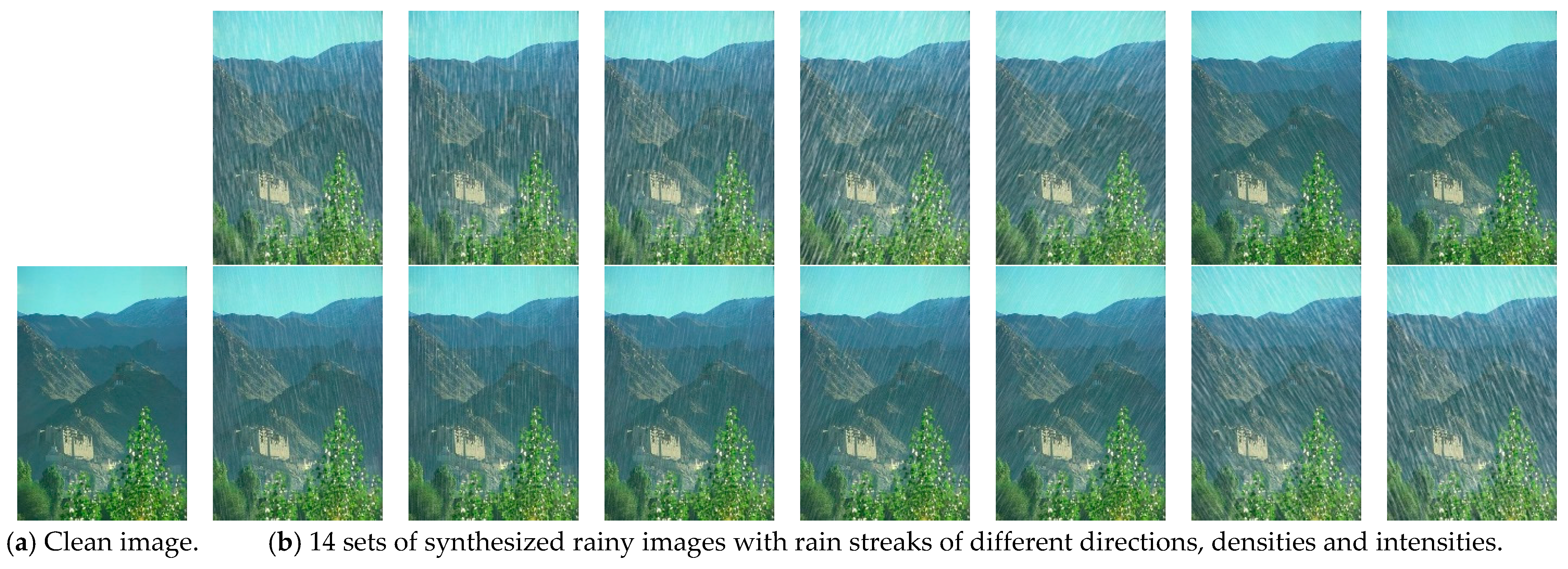
Since it is difficult to obtain clean images corresponding to real-world rainy images, we use synthetic rain images to train our model. We use 12,600 of the 14,000 synthetic images provided by Fu et al. [23] for training the model and 1400 for testing. The dataset was created using each clean image to generate 14 rainy images with different rain streak orientations, shapes, and intensities, as shown in Figure 9. Zhang et al. [26] provided 1200 synthetic images with different rain density conditions for testing. There were also 2800 public images contributed by Fu et al. [25] with varying rain directions and intensities. Zhang et al. [42] provided a Test 100 dataset of different rain directions and densities. We can evaluate the performance of the proposed algorithm under the conditions of rain streak intensity, rain streak direction and different rain densities.

All experiments are performed on a PC with an Intel Core i7-10750H CPU @ 2.60 GHz, 64 GB of RAM and an NVIDIA GeForce GTX 2060 CPU. It takes approximately 7 h to train a proposed model on a synthetic dataset. All methods use the same training and testing datasets. We use stochastic gradient descent (SGD) to minimize the objective function in Formula (5). Motivated by the success of DerainNet [23] and a DDN [25] in rain removal, we use 26 convolution layers followed by the ReLU function. The filter sizes of each layer are 3 × 3, and the filter number in each layer is 16. We use SGD with a weight decay of 10⁻¹⁰ and momentum of 0.9. The training set is 21,600 images, and the minimum batch size is 20. The size of the image patch is 64 × 64 × 3. We set an initial learning rate of 0.1 and divide it by 10 every 100,000 iterations. A total of 210,000 iterations were set to train the model. We first use a large learning rate to quickly obtain an optimal parameter value and then gradually reduce the learning rate by increasing the number of iterations, which ensures that the parameters are excellent and the number of iterations is small. Although the parameters of the proposed model are similar to those of the method in [25], our experimental results show that the proposed model is significantly different from these methods and achieves better results.

4.2. Results

4.2.1. Results on Synthetic Datasets

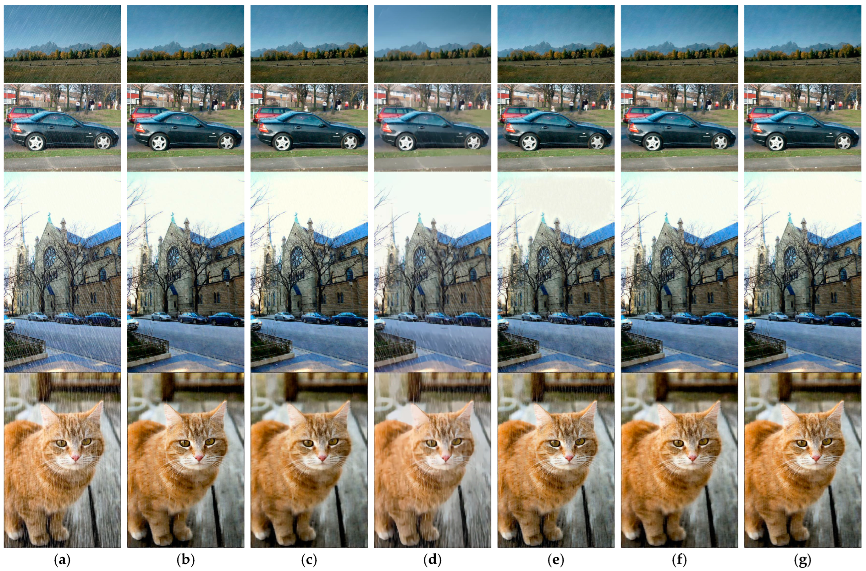
We train a GS filter-based rain removal model on synthetic data and compare it with the methods of references [23,25,37]. In addition, we fix our network structure and compare the effect of removing rain streaks by a Gaussian filter and bilateral filter combined with a deep CNN. We refer to these two models as Gaussian filter-based [32] and bilateral filter-based [34] models. We retrained the compared models using the same dataset for a fair comparison. We first compare them through subjective vision. The test results of our model seem to be more vivid and remove more rain streaks. However, with the increase in rain streak intensity and density, a small amount of rain streak remained in the test results of the Gaussian filter-based and [37] methods.

In addition, we objectively and quantitatively evaluate the test results of the six models through the structural similarity index measure (SSIM) [43] and peak signal-to-noise ratio (PSNR) [44]. We use the SSIM to measure image similarity in terms of brightness, contrast, and structure. The value range of the SSIM is [0, 1]. The larger the SSIM value is, the smaller the distortion of the derained image and the closer it is to the clean image. As shown in

Table 1. Quantitative measurement results using average SSIM on synthesized test images. (The best results are marked in bold.)

Datasets	Rainy Image	Method [23]	Method [25]	Method [37]	Gaussian Filter-Based	Bilateral Filter-Based	Ours
Forest	0.897	0.953	0.953	0.867	0.944	0.951	0.954
Car	0.958	0.970	0.969	0.851	0.961	0.970	0.970
House	0.900	0.955	0.954	0.889	0.927	0.956	0.956
Cat	0.862	0.912	0.915	0.772	0.893	0.917	0.920
Rain 1200 [26]	0.950	0.959	0.959	0.890	0.953	0.958	0.959
Rain 1400 [23]	0.874	0.938	0.937	0.854	0.916	0.938	0.940
Rain 2800 [25]	0.868	0.937	0.934	0.830	0.906	0.934	0.938

, our proposed model achieved comparable or better results than existing methods on all datasets, including images with different rain directions, densities, and rain streak intensities. Our method is effective in removing rain streaks, which enhances the image brightness and contrast after rain removal. For example, the color of the cat image changes more obviously after rain removal (in Figure 10), and the SSIM value increases from 0.862 to 0.920. Our method effectively removes rain streaks in images and prevents color distortion. We calculate the PSNR metrics for the rain removal results produced by the six models, as shown in

Table 2. Average PSNR comparisons on synthetic datasets (dB). (The best results are marked in bold.)

Datasets	Rainy Image	Method [23]	Method [25]	Method [37]	Gaussian Filter-Based	Bilateral Filter-Based	Ours
Forest	27.26	31.35	31.58	24.61	31.34	31.39	31.58
Car	27.31	28.60	28.59	23.89	27.58	28.28	28.68
House	22.31	28.99	28.90	21.46	27.08	29.22	29.15
Cat	21.33	27.85	27.92	20.55	26.54	28.27	28.28
Rain 1200 [26]	27.68	27.29	27.29	24.41	28.51	28.69	28.71
Rain 1400 [23]	23.67	28.17	28.22	22.52	27.37	28.31	28.35
Rain 2800 [25]	22.82	28.16	28.05	21.41	26.63	28.15	28.18

, to evaluate the deraining abilities of the different methods. The PSNR is an evaluation index based on image pixel statistics that measures the quality of the image to be evaluated from a statistical point of view by calculating the difference between the gray values of the pixels of the image to be evaluated and the corresponding pixels of the reference image. Compared with other methods, our model has better rain removal quality. Table 1 and Table 2 report the quantitative comparison results obtained by all competing methods on synthetic datasets with different complexities and different rain patterns. Gaussian filter-based and bilateral filter-based methods and the [25] method are all acceptable for rain removal, but the bilateral filter has a drawback in that the computation is time-consuming. In contrast, our model obtains the best average PSNR and SSIM values for the test data. This result reflects that the model based on the GF filter is effective for rain removal from a single image.

Additionally, the proposed method shows higher improvement, as shown in Figure 11. When the structure of objects in rainy images is similar to rain streaks, it is difficult to completely remove rain streaks and preserve the structure at the same time. Compared with other methods, our method recovers more background images with flexible filter transition bands without removing image details. The white box in each image in the figure represents the enlarged portion of the image. As is again evident in these results, Gaussian filter-based and bilateral filter-based methods preserve the details in the image better. However, the Gaussian filter-based method leaves more rain marks, while the [23,37] methods are over smooth and leave a small number of rain steaks. Our model can completely remove rain streaks while maintaining image object quality, as shown in Figure 11h.

4.2.2. Results on Real-World Datasets

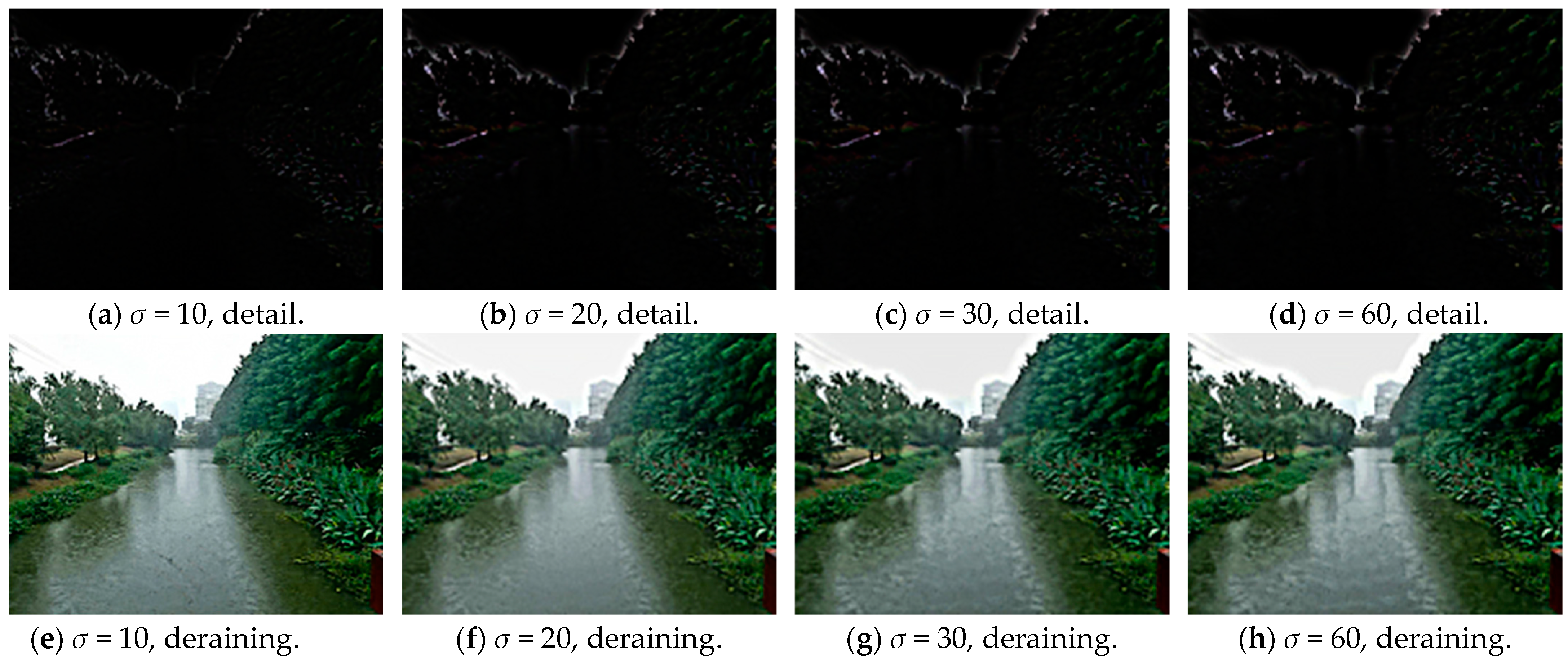
Our proposed model is used to study the removal of rain steaks from real-world images. Four different σ choices are tested: 10, 20, 30, and 60. As shown in Figure 12, if the value of σ increases, the range of morphological artifacts also increases. Morphological artifacts caused by filtering can affect the visual appearance of an image. Therefore, we suppress the generation of morphological artifacts by adjusting the transition band of the GS filter. After conducting many experiments, it is verified that for the real-world data test, σ is set to 10 to obtain images with better quality.

We test the effectiveness and generalization ability of the proposed method by collecting 120 rainy images of the real world from the web and the real dataset Practical 15 provided by Yang et al. [24]. In Figure 13, we compare the single image rain removal results obtained by six models on real-world data. Since we do not have clean images corresponding to real-world rainy images, we use a no-reference metric called the blind image quality index (BIQI) [45] to conduct a quantitative evaluation. This index is designed to provide an image quality score without reference to the ground truth. The lower the BIQI value is, the higher the image quality. As

Table 3. Quantitative measurement results of BIQI on real-world test images. (The best results are marked in bold.)

Datasets	Input	Method [23]	Method [25]	Method [37]	Gaussian Filter-Based	Bilateral Filter-Based	Ours
Leaves	29.23	26.75	26.73	33.70	25.56	26.56	26.61
Passerby	37.69	31.49	30.80	40.14	30.89	32.98	30.80
Bridge	27.96	26.48	24.94	37.84	25.06	27.97	24.82
Bike	29.90	31.02	30.30	37.96	28.22	28.42	28.17
Practical 15 [24]	32.53	28.28	28.18	35.90	29.11	28.81	28.16
Real-world 120	32.11	30.31	29.85	40.10	30.11	31.10	29.76

indicates, the overall BIQI results show that the best quantitative performance is achieved by our proposed method. The DualCNN model [37] does not work well under high-density rainfall conditions. Models based on Gaussian filter and guided filter [23,25] cannot remove rain streaks clearly under heavy rain conditions. On the other hand, the proposed GS-filter-based model works well in all cases. While we use synthetic data to train our GS-filtering-based model, we find that this is sufficient for learning a model that is effective when applied to real-world images. This reflects the better generality of the model based on the GS filter.

Furthermore, as shown in the second row of Figure 13, our method is able to remove rain streaks in the image without color distortion, which the other six methods cannot. We compare the fine structures of the rain removal results produced by the seven models for the real-world data (Figure 14). It is evident that the [25,37,38] methods over-smooth the images, especially in areas with fine structures (Figure 14c,d,g). The main issue of rain streak removal from images is to prevent over-smoothing (or under-clearing) phenomena. Our method preserves more of the fine structure of the image while adequately removing rain streaks. In the case of high rain density and intensity, pursuing the complete removal of rain streaks can easily lead to over-smoothing of the image structure. The method in [38] seeks to completely remove rain streaks, which not only leads to over-smoothing of the results but also color distortion. As shown in Figure 14h, our model is able to remove the thick rain streaks at the lower edge of the image and keep the image background clear, which other methods cannot.

5. Discussion

5.1. Impact of Patch Size

In this section, we test different parameter settings to study their impact on performance. The patch size represents the size of the image patch processed by the model kernel for each input. We use patch sizes of 32 × 32 × 3, 64 × 64 × 3 and 128 × 128 × 3 to train the three models and compare the effect of rain removal. We use the same training data as previously. The testing data include 100 rainy images [42].

Table 4. The average SSIM and PSNR models for different patch sizes.

Patch Size	32 × 32 × 3		64 × 64 × 3		128 × 128 × 3
	SSIM	PSNR	SSIM	PSNR	SSIM	PSNR
Rain 100 test [42]	0.735	15.18	0.867	21.61	0.859	21.79

shows the average SSIM and PSNR values for these three models. Table 4 shows the average SSIM and PSNR values of the three models. As seen, the images with increased patch size to remove rain have higher PSNR. However, the SSIM declines, and increasing the patch size increases the computational complexity due to the need for more convolution operations. According to the SSIM and PSNR results of these three models, we choose to set the patch size = 64 × 64 × 3 for our model.

5.2. Testing Runtime

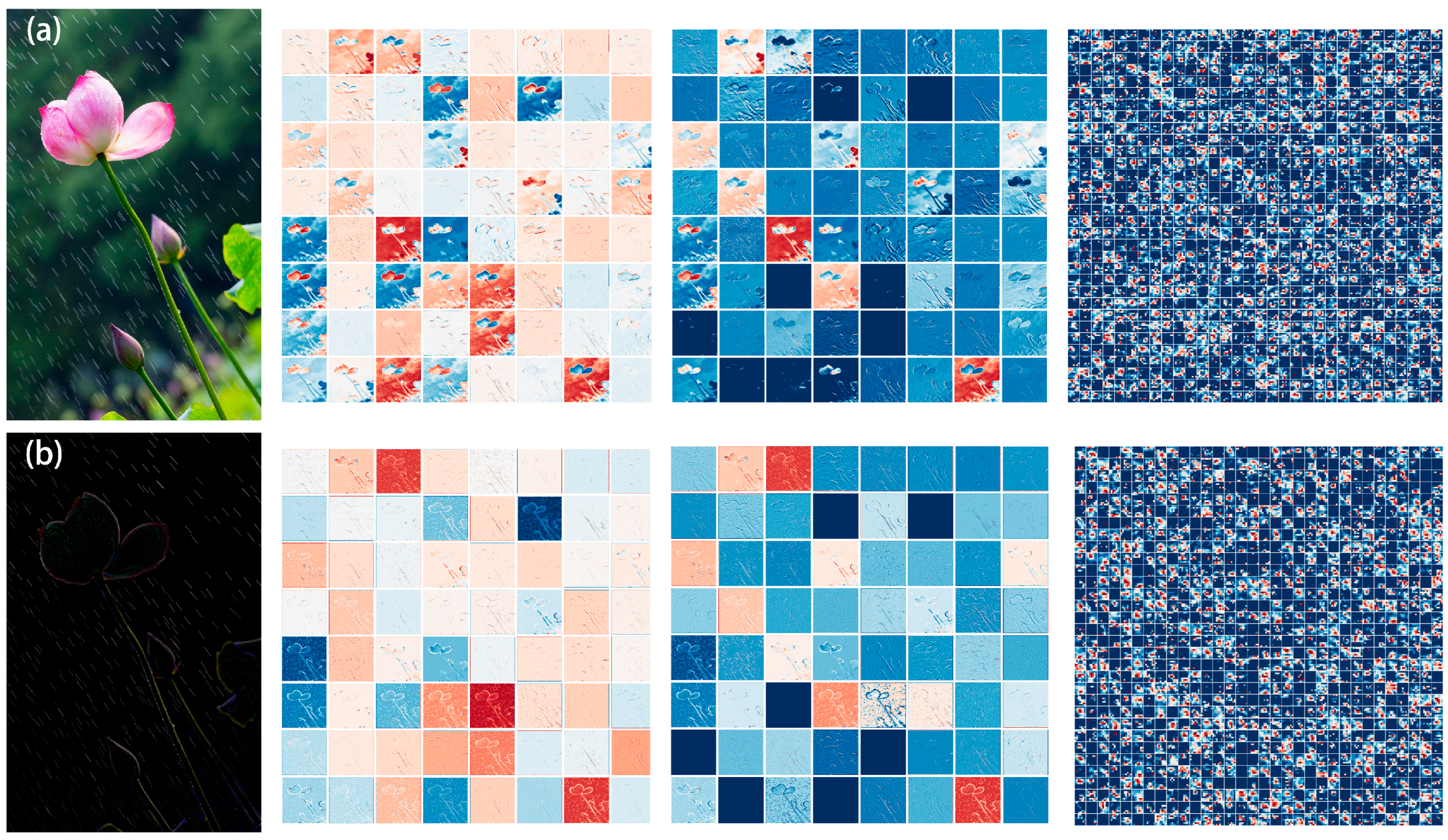
Our proposed algorithm trains the model by feeding the high-frequency parts of rainy images through a GS filter rather than feeding the entire image into the model. We visualize the (the first, third and eighth layers) feature maps for different hidden layers in Figure 15. Figure 15a shows the intermediate result of the model trained on the input whole image. As shown in Figure 15b, the intermediate results of the model trained by inputting the high-frequency part through the GS filter have feature maps that are sparser than the original.

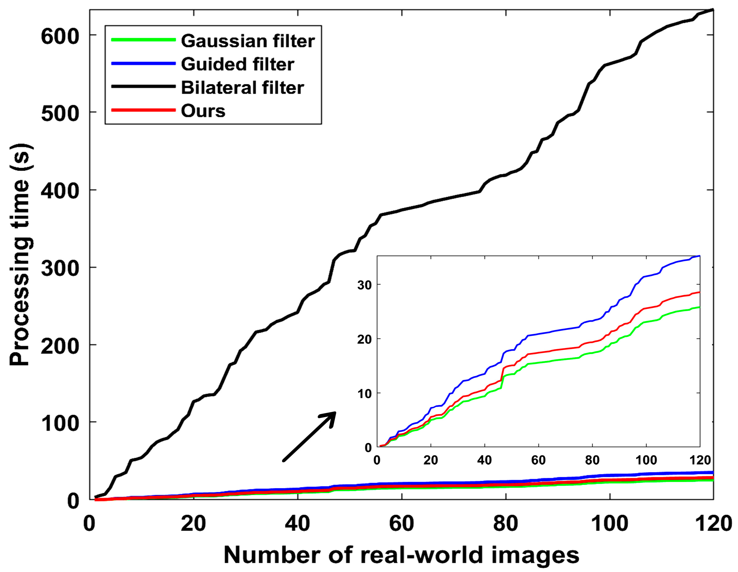
Furthermore, we compare the computational complexity of four filter-based models. The transform domain and average running time of the Gaussian filter, guided filter, bilateral filter and proposed GS filter to process an image are shown in

Table 5. The transform domain and average running time of different filters.

Method	Gaussian Filter	Guided Filter	Bilateral Filter	Ours
Transform domain	Frequency domain	Time domain	Time domain	Time domain
running time (seconds)	0.21	0.29	5.27	0.24

. We compare the time taken by four filter-based models to process 120 real-world images, as shown in Figure 16. The Gaussian filter-based model takes the shortest time to process the given image, and we determine that this is because the Gaussian filter is performed in the frequency domain through the transfer function. The rain removal model is based on the guided filter because the calculation of the guided filter requires a guide image, which increases the number of computations. The bilateral filter can well preserve the edge details of the image and remove rain, but the efficiency of the bilateral filter is not high, and the time spent is relatively long compared to other filters. For real data, the direction of rain is more complex, and the problem of rain removal from a single image becomes more difficult and time-consuming. The proposed GS filter implements filtering in the time domain through a series of convolution operations. However, convolution is more computationally intensive than multiplication, and convolution in the time domain is equal to the product in the frequency domain. Therefore, according to the convolution theorem, the next step is to switch the GS filter to the frequency domain to implement filtering through multiplication operations to reduce the amount of calculation, which is expected to further reduce the required time duration.

6. Conclusions

Our key idea was to propose a GS filter with an adjustable transition band. The proposed GSDerainNet is actually a deep network architecture based on a GS filter. This method can effectively remove rain streaks from a single image while retaining the fine structure of the image object, which is of great significance for drone capture, target detection and automatic driving under rainy weather conditions. Overall, our work makes four main contributions:

• We define the GS filter and give its general mathematical formula. The developed model is flexible and can adjust the GS filtering technique to extract rain features according to the degree of rain streaks in the input image. The range of morphological artifacts produced by filtering is suppressed by adjusting the transition band parameter.
• The whole rainy image does not need to enter the model; only the high-frequency part is input into the model training process, which reduces the number of pixels in the model operation. In addition, under the premise of ensuring the filtering effect, our method has a faster testing speed than models based on guided filters and bilateral filters.
• Our model shows significant improvement compared to five state-of-the-art methods. In both comparison cases of the same model structure with different filters and different model structures, our model retains a finer image object structure and avoids over-smoothing and color distortion.
• Our model has good generalization ability. We train the model on synthetic data, but the model is equally applicable to real-world datasets. Experimental results obtained on public datasets show that the model based on GS filtering has obvious advantages in terms of image quality and computational efficiency.

The frequency response of the proposed GS filter has a flat filtering band and a smooth transition band, which makes the filtering results more accurate. The GS filter flexibly adjusts the passband ripple, passband edge, stopband ripple and stopband edge to improve the visual quality achieved by removing rain streaks from a single image. Therefore, the proposed GSDerainNet model clearly distinguishes rain streaks and background details and prevents color distortion.

Over-smoothing an image can cause object boundaries to become blurred, reducing the performance of computer vision systems. Our model preserves the fine structures of image objects while removing rain streaks. An extensive experiment demonstrates that our method outperforms state-of-the-art methods designed for single image rain removal. In addition to removing rain streaks from a single image, the proposed filter has many applications. For example, this filter can be used for image denoising and image enhancement (especially with respect to image details). We will investigate these applications in future research.

References

1. Xi, Y.; Jia, W.; Miao, Q.; Feng, J.; Liu, X.; Li, F. CoDerainNet: Collaborative Deraining Network for Drone-View Object Detection in Rainy Weather Conditions. Remote Sens. 2023, 15, 1487. [Google Scholar] [CrossRef]
2. Hu, X.; Xu, X.; Xiao, Y.; Chen, H.; He, S.; Qin, J.; Heng, P.-A. SINet: A scale-insensitive convolutional neural network for fast vehicle detection. IEEE Trans. Intell. Transp. Syst. 2018, 20, 1010–1019. [Google Scholar] [CrossRef]
3. Janai, J.; Güney, F.; Behl, A.; Geiger, A.; Graphics, T. Computer vision for autonomous vehicles: Problems, datasets and state of the art. In Foundations and Trends® in Computer Graphics and Vision; Now Publishers Inc.: Delft, The Netherlands, 2020; Volume 12, pp. 1–308. [Google Scholar]
4. Hu, C.; Wang, H. Enhancing Rainy Weather Driving: Deep Unfolding Network with PGD Algorithm for Single Image Deraining. IEEE Access 2023, 11, 57616–57626. [Google Scholar] [CrossRef]
5. Li, R.; Tan, R.; Cheong, L.; Aviles-Rivero, A.; Fan, Q.; Schonlieb, C. Rainflow: Optical flow under rain streaks and rain veiling effect. In Proceedings of the IEEE/CVF International Conference on Computer Vision, Seoul, Republic of Korea, 27 October–2 November 2019; pp. 7304–7313. [Google Scholar]
6. Islam, M.R.; Paul, M. Video Deraining Using the Visual Properties of Rain Streaks. IEEE Access 2022, 10, 202–212. [Google Scholar] [CrossRef]
7. Abdel-Hakim, A.E. A Novel Approach for Rain Removal from Videos Using Low-Rank Recovery. In Proceedings of the 2014 5th International Conference on Intelligent Systems, Modelling and Simulation, Langkawi, Malaysia, 27–29 January 2014; pp. 351–356. [Google Scholar]
8. Dou, Y.; Zhang, P.; Zhou, Y.; Zhang, L. A Tensor Modeling for Video Rain Streaks Removal Approach Based on the Main Direction of Rain Streaks. In Proceedings of the 2020 17th International Computer Conference on Wavelet Active Media Technology and Information Processing (ICCWAMTIP), Chengdu, China, 18–20 December 2020; pp. 380–383. [Google Scholar]
9. Lee, K.-H.; Ryu, E.; Kim, J.-O. Progressive Rain Removal via a Recurrent Convolutional Network for Real Rain Videos. IEEE Access 2020, 8, 203134–203145. [Google Scholar] [CrossRef]
10. Ahn, N.; Jo, S.Y.; Kang, S. Eagnet: Elementwise attentive gating network-based single image de-raining with rain simplification. IEEE Trans. Circuits Syst. Video Technol. 2022, 32, 608–620. [Google Scholar] [CrossRef]
11. Li, Y.; Tan, R.; Guo, X.; Lu, J.; Brown, M.S. Rain streak removal using layer priors. In Proceedings of the IEEE Conference on Computer Vision and Pattern Recognition (CVPR), Las Vegas, NV, USA, 27–30 June 2016; pp. 2736–2744. [Google Scholar]
12. Luo, Y.; Xu, Y.; Ji, H. Removing rain from a single image via discriminative sparse coding. In Proceedings of the IEEE International Conference on Computer Vision (ICCV), Santiago, Chile, 7–13 December 2015; pp. 3397–3405. [Google Scholar]
13. Zheng, X.; Liao, Y.; Guo, W.; Fu, X.; Ding, X. Single-image-based rain and snow removal using multi-guided filter. In Proceedings of the International Conference on Neural Information Processing, Daegu, Republic of Korea, 3–7 November 2013; Springer: Berlin/Heidelberg, Germany, 2013; pp. 258–265. [Google Scholar]
14. Li, Z.; Zheng, J.; Zhu, Z.; Yao, W.; Wu, S. Weighted guided image filtering. IEEE Trans. Image Process. 2015, 24, 120–129. [Google Scholar]
15. Li, Z.; Zheng, J. Single image de-hazing using globally guided image filtering. IEEE Trans. Image Process. 2017, 27, 442–450. [Google Scholar] [CrossRef] [PubMed]
16. Hu, X.; Wang, W.; Pang, C.; Lan, R.; Luo, X. Rain-Density Squeeze-and-Excitation Residual Network for Single Image Rain-removal. In Proceedings of the 2019 Eleventh International Conference on Advanced Computational Intelligence (ICACI), Guilin, China, 7–9 November 2019; pp. 284–289. [Google Scholar]
17. Yang, W.; Tan, R.; Feng, J.; Guo, Z.; Yan, S.; Liu, J. Joint Rain Detection and Removal from a Single Image with Contextualized Deep Networks. IEEE Trans. Pattern Anal. Mach. Intell. 2020, 42, 1377–1393. [Google Scholar] [CrossRef] [PubMed]
18. Wang, Y.; Zhao, X.; Jiang, T.; Deng, L.; Chang, Y.; Huang, T. Rain Streaks Removal for Single Image via Kernel-Guided Convolutional Neural Network. IEEE Trans. Neural Netw. Learn. Syst. 2021, 32, 3664–3676. [Google Scholar] [CrossRef] [PubMed]
19. Jang, Y.; Son, C.; Choo, H. Lightweight Deep Extraction Networks for Single Image De-raining. In Proceedings of the 2021 15th International Conference on Ubiquitous Information Management and Communication (IMCOM), Seoul, Republic of Korea, 4–6 January 2021; pp. 1–4. [Google Scholar]
20. Wang, H.; Xie, Q.; Wu, Y.; Zhao, Q.; Meng, D. Single image rain streaks removal: A review and an exploration. Int. J. Mach. Learn. Cybern. 2020, 11, 853–872. [Google Scholar] [CrossRef]
21. Li, R.; Cheong, L.; Tan, R. Heavy rain image restoration: Integrating physics model and conditional adversarial learning. In Proceedings of the IEEE Conference on Computer Vision and Pattern Recognition (CVPR), Long Beach, CA, USA, 15–20 June 2019; pp. 1633–1642. [Google Scholar]
22. Wang, G.; Sun, C.; Sowmya, A. Erl-net: Entangled representation learning for single image de-raining. In Proceedings of the IEEE International Conference on Computer Vision (ICCV), Seoul, Republic of Korea, 27 October–2 November 2019; pp. 5644–5652. [Google Scholar]
23. Fu, X.; Huang, J.; Ding, X.; Liao, Y.; Paisley, J. Clearing the skies: A deep network architecture for single-image rain removal. IEEE Trans. Image Process. 2017, 26, 2944–2956. [Google Scholar] [CrossRef]
24. Yang, W.; Tan, R.; Feng, J.; Liu, J.; Guo, Z.; Yan, S. Deep joint rain detection and removal from a single image. In Proceedings of the 2017 IEEE Conference on Computer Vision and Pattern Recognition (CVPR), Honolulu, HI, USA, 21–26 July 2017; pp. 1357–1366. [Google Scholar]
25. Fu, X.; Huang, J.; Zeng, D.; Huang, Y.; Ding, X.; Paisley, J. Removing rain from single images via a deep detail network. In Proceedings of the 2017 IEEE Conference on Computer Vision and Pattern Recognition (CVPR), Honolulu, HI, USA, 21–26 July 2017; pp. 3855–3863. [Google Scholar]
26. Zhang, H.; Patel, V.M. Density-aware single image de-raining using a multi-stream dense network. In Proceedings of the 2018 IEEE Conference on Computer Vision and Pattern Recognition (CVPR), Salt Lake City, UT, USA, 18–23 June 2018; pp. 695–704. [Google Scholar]
27. Wang, T.; Yang, X.; Xu, K.; Chen, S.; Zhang, Q.; Lau, R.W. Spatial attentive single-image deraining with a high quality real rain dataset. In Proceedings of the 2019 IEEE Conference on Computer Vision and Pattern Recognition (CVPR), Long Beach, CA, USA, 15–20 June 2019; pp. 12270–12279. [Google Scholar]
28. Wang, H.; Xie, Q.; Zhao, Q.; Meng, D. A model-driven deep neural network for single image rain removal. In Proceedings of the IEEE/CVF Conference on Computer Vision and Pattern Recognition (CVPR), Seattle, WA, USA, 13–19 June 2020; pp. 3103–3112. [Google Scholar]
29. Chen, D.; Chen, C.; Kang, L. Visual Depth Guided Color Image Rain Streaks Removal Using Sparse Coding. IEEE Trans. Circuits Syst. Video Technol. 2014, 24, 1430–1455. [Google Scholar] [CrossRef]
30. He, K.; Sun, J.; Tang, X. Guided image filtering. IEEE Trans. Pattern Anal. Mach. Intell. 2012, 35, 1397–1409. [Google Scholar] [CrossRef] [PubMed]
31. Xu, J.; Zhao, W.; Liu, P.; Tang, X. Removing rain and snow in a single image using guided filter. In Proceedings of the 2012 IEEE International Conference on Computer Science and Automation Engineering (CSAE), Zhangjiajie, China, 25–27 May 2012; pp. 304–307. [Google Scholar]
32. Yeh, C.H.; Liu, P.; Yu, C.; Lin, C. Single image rain removal based on part-based model. In Proceedings of the 2015 IEEE International Conference on Consumer Electronics, Taipei, Taiwan, 6–8 June 2015; pp. 462–463. [Google Scholar]
33. Shi, Z.; Li, Y.; Zhao, M.; Feng, Y.; He, L. Multi-stage filtering for single rainy image enhancement. IET Image Process. 2018, 12, 1866–1872. [Google Scholar] [CrossRef]
34. Tomasi, C.; Manduchi, R. Bilateral filtering for gray and color images. In Proceedings of the International Conference on Computer Vision (ICCV), Bombay, India, 4–7 January 1998; pp. 839–846. [Google Scholar]
35. Pal, N.S.; Lal, S.; Shinghal, K. A Visibility Restoration Framework for rainy images by using L0 gradient minimization and Bilateral Filtering. In Proceedings of the 2018 International Conference on Advances in Computing, Communication Control and Networking (ICACCCN), Uttar Pradesh, India, 12–13 October 2018; pp. 848–852. [Google Scholar]
36. Du, S.; Liu, Y.; Ye, M.; Xu, Z.; Li, J.; Liu, J. Single image deraining via decorrelating the rain streaks and background scene in gradient domain. Pattern Recognit. 2018, 79, 303–317. [Google Scholar] [CrossRef]
37. Pan, J.; Sun, D.; Zhang, J.; Tang, J.; Yang, J.; Tai, Y.; Yang, M. Dual Convolutional Neural Networks for Low-Level Vision. Int. J. Comput. Vis. 2022, 130, 1440–1458. [Google Scholar] [CrossRef]
38. Ye, Y.; Chang, Y.; Zhou, H.; Yan, L. Closing the loop: Joint rain generation and removal via disentangled image translation. In Proceedings of the IEEE/CVF Conference on Computer Vision and Pattern Recognition (CVPR), Nashville, TN, USA, 20–25 June 2021; pp. 2053–2062. [Google Scholar]
39. Kang, L.W.; Lin, C.W.; Fu, Y. Automatic single-image-based rain streaks removal via image decomposition. IEEE Trans. Image Process. 2011, 21, 1742–1755. [Google Scholar] [CrossRef]
40. Huang, D.; Kang, L.; Wang, Y.; Lin, C. Self-learning based image decomposition with applications to single image denoising. IEEE Trans. Multimed. 2013, 16, 83–93. [Google Scholar] [CrossRef]
41. Ioffe, S.; Szegedy, C. Batch Normalization: Accelerating Deep Network Training by Reducing Internal Covariate Shift. In Proceedings of the International Conference on Machine Learning, Lille, France, 6–11 July 2015; pp. 1–11. [Google Scholar]
42. Zhang, H.; Sindagi, V.; Patel, V.M. Image De-Raining Using a Conditional Generative Adversarial Network. IEEE Trans. Circuits Syst. Video Technol. 2020, 30, 3943–3956. [Google Scholar] [CrossRef]
43. Wang, Z.; Bovik, A.C.; Sheikh, H.R.; Simoncelli, E.P. Image quality assessment: From error visibility to structural similarity. IEEE Trans. Image Process. 2004, 13, 600–612. [Google Scholar] [CrossRef] [PubMed]
44. Huynh-Thu, Q.; Ghanbari, M. Scope of validity of PSNR in image/video quality assessment. Electron. Lett. 2008, 44, 800–801. [Google Scholar] [CrossRef]
45. Moorthy, A.K.; Bovik, A.C. A two-step framework for constructing blind image quality indices. IEEE Signal Process. Lett. 2010, 17, 513–516. [Google Scholar] [CrossRef]
Figure 1. Rain removal results corresponding to different filters with the same model structure. (a) The rainy image. (b) Results from the guided filter. (c) Gaussian filter. (d) Bilateral filter. (e) Ours.
Remotesensing 15 04825 g001
Figure 2. Frequency responses of the GS low-pass filter with different transition band parameters.
Remotesensing 15 04825 g002
Figure 3. Frequency responses of the two-dimensional GS filter with different transition band parameters and cutoff scale parameters. (a) Frequency responses of the two-dimensional GS filter with different cutoff scale parameters under the same transition band parameters. (b) Frequency responses of the two-dimensional GS filter with the same cutoff scale parameters for different transition band parameters.
Remotesensing 15 04825 g003
Figure 4. The proposed model framework for single image rain removal.
Remotesensing 15 04825 g004
Figure 5. Comparison results obtained for the filtered low-frequency parts of the clean image and the synthesized rainy image. (a,f) Clean image. (b,g) The low-frequency part of the clean image after GS filtering. (c,h) Synthesized rainy image with rain streaks of different directions, densities and intensities. (d,i) The low-frequency part of the rainy image after GS filtering. (e,j) The difference between the low-frequency part of the clean image and the low-frequency part of the rainy image.
Remotesensing 15 04825 g005
Figure 6. Example base and detail layers of two synthesized images. We use GS filtering as the low-pass filter to generate the results. (fj) Statistical histograms of the three-channel (R, G, B) pixel values corresponding to (ae).
Remotesensing 15 04825 g006aRemotesensing 15 04825 g006b
Figure 7. Effects of different transition band parameters on the morphological artifacts of the GS filtering results at the same cutoff frequency. (a,h) show the synthesized rainy image and the corresponding clean image. (bg) and (in) represent the low- and high-frequency parts obtained after GS filtering, respectively; these parts correspond to different transition band parameters at the same cutoff frequency.
Remotesensing 15 04825 g007
Figure 8. The execution process of the GSDerainNet algorithm.
Remotesensing 15 04825 g008
Figure 9. Examples of synthesized rainy images. The image in the second row and first column is the clean image, and the remaining images are various synthesized images.
Remotesensing 15 04825 g009
Figure 10. Comparison of qualitative and quantitative results on four rainy images sampled from synthetic datasets. (a) Rainy images. (bd) represent the rain removal results of the models of Fu et al. [23], Fu et al. [25] and Pan et al. [37] respectively. (e,f) represent the rain removal results of the Gaussian filter-based and bilateral filter-based models respectively. (g) Ours. Four DL-based methods with better quality and a state-of-the-art dual convolutional neural network method are selected for comparison. Each row of subfigures represents the comparison of the results of six models for removing rain streaks with different directions, densities, and intensities. The quantitative results are shown in Table 1 and Table 2.
Remotesensing 15 04825 g010
Figure 11. Comparison among the fine structures of the images obtained after performing rain streak removal with the six models. (a) Rainy image. (b) Clean image. (ce) represent the rain removal results of the models of Fu et al. [23], Fu et al. [25] and Pan et al. [37] respectively. (f,g) represent the rain removal results of the Gaussian filter-based and bilateral filter-based models re-spectively. (h) Ours.
Remotesensing 15 04825 g011aRemotesensing 15 04825 g011b
Figure 12. Effects of morphological artifacts in the high-frequency layers on the obtained results. (ad) represent the high-frequency detail layers filtered by the GS filter with different transition bands. (eh) represent the rain streaks removal results corresponding to different transition bands of the GS filter.
Remotesensing 15 04825 g012
Figure 13. Generalization performance comparison among all competing methods on typical real test images with rain streaks from internet data. (a) Rainy images. (bd) represent the rain removal results of the models of Fu et al. [23], Fu et al. [25] and Pan et al. [37] respectively. (e,f) represent the rain removal results of the Gaussian filter-based and bilateral filter-based models respectively. (g) Ours. The red boxes in the first column of images represent severe interference from rain streaks. The white boxes in other images represent the enlarged portion of the image.
Remotesensing 15 04825 g013aRemotesensing 15 04825 g013b
Figure 14. Comparison of the fine structure of the rain removal results of the seven methods. (a) Rainy image. (bd) represent the rain removal results of the models of Fu et al. [23], Fu et al. [25] and Pan et al. [37] respectively. (e,f) represent the rain removal results of the Gaussian filter-based and bilateral filter-based models respectively. (g) represents the rain removal results of the model of Ye et al. [38]. (h) Ours. The white box in each image in the figure represents the enlarged portion of the image. The portion of the image in the red box contains relatively intense rain streaks running down the umbrella.
Remotesensing 15 04825 g014aRemotesensing 15 04825 g014b
Figure 15. Feature map visualization. (a) Feature maps of the entire image input model. (b) Feature maps of the high-frequency part of the input model.
Remotesensing 15 04825 g015
Figure 16. Comparison of the run times achieved by the four models in the real data test. The small image indicated by the arrow represents a zoomed-in part of the image.
Remotesensing 15 04825 g016