Global Scale Inversions from MOPITT CO and MODIS AOD

Abstract

Top-down observational constraints on emissions flux estimates from satellite observations of chemical composition are subject to biases and errors stemming from transport, chemistry and prior emissions estimates. In this context, we developed an ensemble data assimilation system to optimize the initial conditions for carbon monoxide (CO) and aerosols, while also quantifying the respective emission fluxes with a distinct attribution of anthropogenic and wildfire sources. We present the separate assimilation of CO profile v9 retrievals from the Measurements of Pollution in the Troposphere (MOPITT) instrument and Aerosol Optical Depth (AOD), collection 6.1, from the Moderate Resolution Imaging Spectroradiometer (MODIS) instruments. This assimilation system is built on the Data Assimilation Research Testbed (DART) and includes a meteorological ensemble to assimilate weather observations within the online Community Atmosphere Model with Chemistry (CAM-chem). Inversions indicate an underestimation of CO emissions in CAMS-GLOB-ANT_v5.1 in China for 2015 and an overestimation of CO emissions in the Fire INventory from NCAR (FINN) version 2.2, especially in the tropics. These emissions increments are consistent between the MODIS AOD and the MOPITT CO-based inversions. Additional simulations and comparison with in situ observations from the NASA Atmospheric Tomography Mission (ATom) show that biases in hydroxyl radical (OH) chemistry dominate the CO errors.

1. Introduction

The goal of atmospheric data assimilation (DA) is to accurately determine the state of the atmosphere, including its gas-phase and aerosol chemical composition, by optimally and objectively combining observations and model simulations [1,2,3]. As pointed out by Bocquet et al. [4], there are few studies of joint meteorological and chemical data assimilation within models that explicitly represent meteorological processes and chemical transformations.

Satellite-based remote-sensing instruments produce large amounts of valuable atmospheric composition data that can be used in assimilation. For instance, the aerosol optical depth (AOD) is available from operating instruments including low Earth orbit satellite sensors, such as the Moderate Resolution Imaging Spectroradiometer (MODIS), the Visible/Infrared Imager Radiometer Suite (VIIRS), and the Multi-Angle Imaging Spectroradiometer (MISR). There have been numerous studies on the feasibility of assimilating aerosol observations to improve the initial conditions for aerosol forecasting [5,6,7]. The choice of control variables is important since AOD measurements are used to initialize a dozen aerosol mass concentrations for which background error statistics are difficult to characterize (e.g., [8]). Schutgens et al. [9] performed the assimilation of AERONET data using a Local Ensemble Transform Kalman Filter (LETKF), which presents an efficient way to model a background error covariance that varies in space and time. In the context of air quality (AQ) forecasting, both PM${}_{2.5}$ and MODIS AOD have been assimilated in Chemistry Transport Models (CTM) (e.g., [10,11]). Pagowski and Grell [12] compared the 3D-VAR and the ensemble Kalman filter (EnKF) assimilation methods for the assimilation of PM${}_{2.5}$ and found that when meteorology alone was perturbed, the ensemble spread was too small to accurately represent the model errors. This points to the problem of representing model error in chemical data assimilation, since CTMs are sensitive to errors in emissions and aerosol models are too simplistic for computational purposes. Schwartz et al. [13] introduced a hybrid variational-ensemble DA system and found that an important limitation of the system was the small ensemble spread. To overcome these difficulties and include meteorology ensembles and perturbations in the aerosol emissions sources, one can use adaptive inflation methods to correct the ensemble spread [14,15]. The better quantification of emissions uncertainties was also introduced in the 3D-Var framework by increasing the background error variance of the accumulation and Aitken mode aerosols, which improved the quality of the analyses [16]. The influence of initial condition (IC) optimization fades with time and the pollutant field at the surface because of emissions and other parameters such as chemical reactivity and deposition velocity [17].

Following the pioneering work of Elbern et al. [18] and Miyazaki et al. [19], more work has been dedicated to simultaneously optimizing the initial conditions and the associated emissions, where the emission increments act as an improved boundary condition during the forecast [20] and the system includes additional constraints from the simultaneous assimilation of different species [21,22]. The latter study [22] pointed out limitations due to the treatment of model error in nonlinear chemical processes and the lack of constraints on volatile organic compounds’ (VOCs) ICs and emissions. Ma et al. [23] assimilated surface measurements of gas-phase species (SO${}_2$, NO${}_2$, O${}_3$, CO) and aerosols (PM${}_{2.5}$, PM${}_{10}$), along with with MODIS AOD, and found that the emissions update interval may be an important factor for CO in EnKF emission inversion studies. They concluded that the posterior emissions could converge to a relatively stable state and that the updated anthropogenic emissions can improve the model forecasts. This is consistent with Gaubert et al. [24], in which the Measurement of Pollution in the Troposphere (MOPITT) CO assimilation showed improved CO forecasts and analyses when compared to independent aircraft observations when the CO ICs and emissions were jointly optimized.

Global aerosol, chemical, and meteorological reanalyses are consistently produced within the same DA infrastructure [25,26,27,28] to better understand the role of aerosols and chemistry in the climate system. A common approach in gas-phase chemical data assimilation systems is to estimate atmospheric states and/or emissions using variational [29,30,31,32,33,34] and ensemble Kalman filter approaches [19,35,36,37,38], often with offline CTMs. Notable exceptions include using coupled chemistry–meteorology DA for stratospheric application [39], for the upper atmosphere [40]. Within the Monitoring Atmospheric Composition and Climate (MACC) and the Copernicus Atmosphere Monitoring Service (CAMS) European projects, global chemical, aerosols, and meteorological observations are assimilated within the Composition-IFS Integrated Forecasting System (IFS) 4D-Var system [28,41,42,43,44]. Despite the assimilation of many observations of different species and satellite platforms, the impact of the data assimilation is very limited near the surface, especially for short-lived species such as NO${}_2$ [45]. Recent developments include the assimilation of Tropospheric Monitoring Instrument (TROPOMI) total column CO in the CAMS system, which alleviates the low CO bias in the free troposphere, especially when assimilating clear-sky TROPOMI CO retrievals [46].

Attributing CO sources is complicated by its strong coupling with atmospheric chemistry via the hydroxyl radical (OH), which acts as both a strong source (via methane and VOCs oxidation) and the main chemical sink of CO. An ensemble of 26 global Chemistry Transport Models (CTM) has shown that CO is underestimated against surface observations and satellite retrievals from MOPITT. While all the models were using the same CH${}_4$ field and emissions, the comparison showed that the variation in OH explained around 80% of the inter-model variance in CO [47]. Other differences in CO were attributable to different representations of VOC emission sources, while meteorology appeared to be less important for large-scale budgets. Later, Voulgarakis et al. [48] compiled model simulations of OH and CH${}_4$ lifetimes from the Atmospheric Chemistry and Climate Modeling Intercomparison Project (ACCMIP) [49] and found large differences in the inter-model estimations of OH and CH${}_4$ lifetimes. Furthermore, Naik et al. [50] showed that the ACCMIP multimodel mean OH concentration is overestimated by 5 to 10%, because OH concentrations are overestimated in the northern hemisphere. The POLARCAT Model Inter-Comparison Project (POLMIP) indicated that arctic OH differences are a larger source of inter-model variability than transport differences [51]. Conversely, assimilating MOPITT in such a coupled CTM reduces this bias [52], while Strode et al. [53] found that removing biases in O${}_3$ and water vapor, as well as reducing northern hemisphere NO${}_x$, can also effectively reduce the global mean OH by 18%. In response to this, there has been a strong motivation to elucidate the role of individual driving factors controlling the OH budget [48,54].

Observationally derived OH estimates imply that (1) the global and annual average tropospheric methane lifetime ($\tau$) is 9.5 years [55], (2) the interannual variability is small, by 1 to 3% [56], and (3) the northern hemisphere to southern hemisphere (N/S) ratio is close to 1 [57], with a ratio of 0.97 ± 0.12 for the years 2004–2011 [58]. Zhao et al. [59] used the Chemistry-Climate Model Initiative (CCMI)-modeled OH and indeed found large sensitivities of the simulated CH${}_4$ to the use of alternative OH fields that have different spatial and temporal distributions and overall magnitude. Gaubert et al. [60] argued that the observed 20% global decline in CO burden during the 2002–2013 period, due to the effective implementation of pollution control technologies and regulations, has also resulted in increased CH${}_4$ oxidation by OH, corresponding to a ∼8% shorter CH${}_4$ lifetime and higher CO chemical production. Nguyen et al. [61] followed this work with simple chemistry box model calculations and suggested that there can be a 25% bias in methane source estimates when chemical feedbacks through OH are neglected. The comparison of free running simulations with data assimilation and prescribed meteorology through nudging implies that while water vapor plays an important role as a source of OH, and therefore impacts global OH abundance, it does not determine the modeled long-term OH trend [24,60,62]. Zhang et al. [63] optimized the annual hemispheric concentrations of tropospheric OH following the assimilation of GOSAT CH${}_4$ and found a reduction in OH concentrations that was mostly in the northern hemisphere, leading to an N/S ratio of 1.02 ± 0.05 in the posterior estimate, compared to 1.16 in the prior estimate. Recently, CH${}_4$ inversions have been carried out using an OH that is constrained by precursor observations (CO, CH${}_2$O), which resulted in better agreement with the MCF-based OH inversions [64]. It confirms the results from earlier studies that the assimilation of precursor emissions usually improves OH metrics such as estimates of the CH${}_4$ lifetime and associated N/S ratios closer to 1 [52,65,66,67]. Müller et al. [68] performed IASI CO inversions with alternative distributions of the N/S ratio and different global OH and showed that the varying hemispheric mean OH level has a strong impact on posterior emission estimates. The CO inversions made with offline chemistry will scale the CO emissions according to the OH distribution, and lower OH, especially in the northern hemisphere, leads to a better CO match with independent observations.

In this context, we developed an ensemble data assimilation framework to optimize the CO initial conditions in an online and interactive atmospheric chemistry model. The goal is to reduce potential biases in OH, transport, and other model-related systematic errors that affect CO and thus the posterior emissions. We presented in a previous study the posterior emission fluxes with a focus on anthropogenic sources in East Asia in May 2016, during the Korea–United States Air Quality (KORUS-AQ) campaign in South Korea [24]. The CO assimilation in an interactive CTM provided constraints on OH, hydroperoxyl radical (HO${}_2$), and O${}_3$ through the joint optimization of CO initial conditions and emissions.

This paper is structured as follows. We introduce the modeling and assimilation framework as well as the assimilated observations and conducted experiments in Section 2. We present the global-scale results of CO inversion experiments for August 2015 in Section 3, including its evaluation with Fourier transform spectrometer observations of the dry-air tropospheric column-averaged mole fraction of CO from the Network for Detection of Atmospheric Composition Change (NDACC). The results for AOD are presented in Section 4. In Section 5, we investigate the sensitivities in deterministic CAM-chem simulations, to scaled OH and posterior emissions, and we further evaluate with MOPITT CO and MODIS AOD level 3 monthly observations. In the following Section 6, we compare the CAM-chem simulations of CO, OH, and HO${}_2$ to the NASA Atmospheric Tomography Mission (ATom). Finally, we discuss our findings in the larger context in Section 7 and the main points are summarized in Section 8.

2. Methods and Observations

2.1. Community Atmosphere Model with Chemistry

We employ the Community Atmosphere Model with Chemistry (CAM-chem), the atmospheric chemistry constituent of the Community Earth System Model (CESM) version 2.2 [69]. This current version uses the finite volume dynamical core at a spatial resolution of 0.95$°$ in latitude by 1.25$°$ in longitude and with 32 vertical layers [70,71]. The Modal Aerosol Model (MAM4) [72,73] is used to represent aerosols over four modes and includes secondary organic aerosols estimated by the Volatility Basis Set (VBS) [71]. The gas-phase chemistry is represented by the MOZART Tropospheric and Stratospheric (TS1) scheme [74]. Following Gaubert et al. [24], we employ the heterogeneous aerosol uptake coefficient ($\gamma$) of 0.1 for HO${}_2$, with the reaction producing H${}_2$O instead of H${}_2$O${}_2$. We update the nitric acid trihydrate (NAT) particle number densities from 0.01 to 10${}^{-5}$ cm${}^{-3}$, which increases the denitrification rate in the stratosphere, resulting in the higher catalytic destruction of stratospheric ozone by chlorine [75]. The Community Land Model version 5 (CLM5) model is active and coupled with the atmosphere [76]. The dry deposition of aerosols and gases as well as biogenic emissions are calculated online in CLM5. Specifically, the Model of Emissions of Gases and Aerosols from Nature (MEGAN v2.1) is used for biogenics [77] and the wet deposition of gases and aerosols is estimated from the Neu and Prather [78] parameterization.

The CAMS-GLOB-ANT_v5.1 inventory was released in spring 2021 and is used for anthropogenic emissions [79]. The dataset is derived from the spatial distribution and monthly emissions (2000 to 2015) of version 5 of the Emissions Database for Global Atmospheric Research (EDGAR v5) from the European Commission Joint Research Centre [80]. Values are extrapolated to 2021 using trends calculated from version 2 of the Community Emissions Data System (CEDS) [81]. It also includes updated ship and aircraft emissions. The emission’s seasonal cycle is derived from monthly adjustments provided by CAMS-GLOB-TEMPO. Daily biomass burning emissions are estimated by the Fire INventory from NCAR [82,83] version 2.2 (FINNv2.2). Among other datasets, the inventory is derived by active fire detection from both VIIRS and MODIS.

We also perform deterministic CAM-chem simulations to assess the differences in using prior and posterior emissions (

Table 1. Deterministic CAM-chem simulations.

Simulation	Anthro	Fire	Notes
CAM-chem-ref	CAMS-GLOB-ANT_v5.1	FINN2.2	reference
CAM-chem-post	CAMS-GLOB-ANT_v5.1	FINN2.2	posterior CO emi.
CAM-chem-post-aer	CAMS-GLOB-ANT_v5.1	FINN2.2	posterior POM and BC emi.
CAM-chem-O1D	CAMS-GLOB-ANT_v5.1	FINN2.2	JO(${}^1$D) reduced by 10%

). The CAM-chem simulated temperature as well as the zonal and meridional winds are nudged to the Modern-Era Retrospective Analysis for Research and Applications version 2 [84], as in recent studies [85,86]. The nudging is performed at every physical time step (30 min) with a Newtonian relaxation of 6 h and reading input files at the highest possible temporal frequency of 3 h [87].

In all CAM-chem simulations, the sea–ice interfaces and ocean are prescribed from a daily analysis of sea surface temperatures (SST) at 0.25$°$ × 0.25$°$ spatial resolution. The dataset is derived from in situ observations and the Advanced Very High Resolution Radiometer (AVHRR) SST observations [88].

2.2. Data Assimilation Research Testbed

DART is an open source community software for efficient ensemble data assimilation, developed and maintained at the National Center for Atmospheric Research [89]. Global meteorological reanalyses were performed within the Community Atmosphere Model (CAM) or CAM6 + DART [90]. Our chemical data assimilation system is built upon CAM6 + DART with the inclusion of online chemistry to efficiently assimilate chemical observations [24,52]. Briefly, the first step of the filter is to run a 30 member ensemble of CAM-chem simulations with different initial conditions, forcing files such as emissions as well as various model parameters. The analysis step is the assimilation of observations using a deterministic ensemble square root filter, the ensemble adjustment Kalman filter (EAKF) [91,92]. We apply multiplicative covariance inflation to the ensemble before the analysis step to optimally adjust the ensemble spread. The adaptive inflation parameters vary in space and time [93] and are calculated following the updated algorithm from Gharamti [94]. The spatial localization [95] is set to a half width value of ∼600 km (0.1 radians) horizontally and of about 1200 m in the vertical for both meteorological and chemical observations.

2.3. Assimilation Experiments

Our numerical simulations include the assimilation of MOPITT CO (MOPITT-DA), MODIS AOD (MODIS-DA), and baseline meteorological observations (Control-DA). The ensemble consists of 30 CAM-chem runs with different initial conditions and model parameters, including emissions and nudging strength values. The ensemble spinup simulation is initialized from a CAM-chem deterministic simulation on 21 July 2015. During the CAM-chem ensemble spinup period, the temperature and the wind velocity components are nudged towards the CAM6 + DART reanalysis ensemble mean [90], at every physical step (30 min). To generate a dynamical spread, we perturb the global strength Q of the nudging so that the ensemble mean is a nudging of Q = 0.4 with a standard deviation of 0.15, which corresponds to relaxation times mostly between 10 and 20 h. For this simulation and all of the following experiments, the global dust emission factor is perturbed by 10% and the sea salt global emission factor is perturbed by 25%. A different noise distribution (estimated as in Gaubert et al. [96]) is applied to CO, VOC, and aerosol emissions for biomass burning (BB), with a decorrelation length of 250 km, and for anthropogenic direct emissions, with a decorrelation length of 500 km. Thus, anthropogenic and BB CO sources are completely uncorrelated in the prior ensemble. Using an ensemble for meteorological data assimilation allows the characterization of errors in the model horizontal and vertical dynamics and physics. The meteorological data assimilation starts on 28 July 2015 and will serve as a control run, so the nudging to the CAM6 + DART reanalysis is turned off. We initialize the MOPITT-DA and the MODIS-DA assimilation experiments on 1 August 2015 from the control-run.

DART is also designed to handle both the spatial and the “variable localization” [97]. The variable localization restricts the impact of an observation to only relevant model fields. For instance, the “variable localization” means that the MOPITT assimilation impacts only the chemical state vector (i.e., CO and CO emissions), with no correction on the meteorological state vector (U, V, T, Q, Ps).

Table 2. State vector employed in assimilation experiments.

	Control-DA	MOPITT-DA	MODIS-DA
State vector (Met.)	U, V, T, Q, Ps	U, V, T, Q, Ps	U, V, T, Q, Ps
State vector (Chem.)		CO	MMR${}_{a1}$, MMR${}_{a2}$, MMR${}_{a3}$,MMR${}_{a4}$
State vector (Chem. fluxes)		SFCO${}_{CAMS}$, SFCO${}_{FINN}$	SFBC, SFPOM

shows the state vectors used in the different experiments. All experiments assimilate meteorological observations in a consistent manner, including for the AOD and CO assimilation runs. In the MOPITT-CO experiment, the CO initial conditions are optimized and the anthropogenic (SFCO${}_{CAMS}$) and fire (SFCO${}_{FINN}$) emissions are updated following the method presented in Gaubert et al. [24]. Briefly, the persistence of the emissions is assumed since there is no model for emissions. However, the relative increments are applied by source for the next few days of the input emission fluxes files with a decreasing weight over time. We use a $\tau$ of 5 days for fires and 8 days for the anthropogenic source. The native temporal resolution of the anthropogenic emissions is monthly, so we consider impacts up to 16 days (2$\tau$). To discriminate sources, only fire emissions are updated if their fluxes constitute more than 10% of the CAMS emissions for a given grid cell. Otherwise, only SFCO${}_{CAMS}$ are updated. For aerosol DA, only the black carbon (SFBC) and primary organic matter (SFPOM) emissions are optimized, using the same CO tag ratio to determine which of the CAMS or FINN emission files will be updated for each grid cell. In the MODIS-DA experiment, the total mass mixing ratios of the 4 bins are in the state vector. The 16 different aerosol species and the 4 number variables are scaled after the analysis step.

2.4. Observations

2.4.1. MOPITT

MOPITT is a radiometer instrument that measures CO in both thermal and short-wave infrared bands [98]. We present here our first assimilation of the latest (V9J) MOPITT multispectral retrievals [99]. V9J retrievals feature a revised cloud detection algorithm that now includes observations over highly polluted scenes, with relatively high aerosol optical depths, that were previously treated as cloudy scenes [100]. The adopted algorithm results in greater retrieval coverage over land, particularly over polluted scenes such as the Amazon Basin during the fire season and the North China Plain. While we follow the same approach as in previous studies, by assimilating daytime-only joint retrieval profiles [24], we now only employ the measurement error covariance as the observation error instead of the total retrieval error covariance. This is because the model is smoothed by the averaging kernel during the forward operator, so the smoothing error (which is included in the retrieval error covariance) is already taken into account [101]. The comparison of the two approaches indicates that only including the measurement error allows for a better fit of the MOPITT observations.

2.4.2. MODIS

We use the AOD dataset from the MODIS collection 6.1 [102], from both the Terra and Aqua satellites and retrieved with the Deep Blue algorithm. The dataset is processed to achieve low systematic bias and random error for use in data assimilation, following 3 steps: (1) a quality assurance (QA) analysis, (2) an empirical correction, and (3) aggregation [103,104,105]. The QA procedure includes standard error checks, buddy checks, and QA flag checks. The standard error check is designed to identify cloud-contaminated pixels by evaluating the spatial variation of the MODIS AOD, buddy checks remove isolated pixels, and only data flagged as good and best with a cloud fraction lower than 80% are used. The empirical correction is then applied to further reduce the biases from cloud artifacts, surface wind speed effects, and aerosol microphysics effects. The data are then averaged on a 0.5$°$ × 0.5$°$ grid for a 6-hourly time window.

We also use a MODIS AOD level 3 climatology for the evaluation of deterministic CAM-chem simulations. The AOD monthly data are from the Terra MODIS Collection 6.1 Monthly Level 3 (1$°$ × 1$°$) Combined Dark Target and Deep Blue product [106], which has been regridded to the CAM6 grid via bilinear interpolation.

2.4.3. Network for Detection of Atmospheric Composition Change

To further evaluate the impacts of the CO assimilation, we compare the simulated CO with ground-based Fourier transform infrared spectrometer (FTIR) CO observations at multiple sites across the world [86]. This dataset is part of the NDACC (http://ndacc.org, accessed on 30 September 2023) Infrared Working Group (IRWG, https://www2.acom.ucar.edu/irwg, accessed on 30 September 2023)). The sites are located in either close to urban areas or in remote locations. The FTIR acquires direct-sun spectra under cloud-free conditions in selected spectral regions through the mid-infrared with a nominal spectral resolution of 0.004 cm${}^{-1}$. For CO, a liquid-nitrogen-cooled InSb (∼1850–6000 cm${}^{-1}$) and narrow bandpass filter are used to yield typical accuracy and precision of about 3% and 1%, respectively. The modeled vertical profiles are smoothed with the FTIR averaging kernels and a priori vertical profiles to account for the FTIR altitude sensitivity. For the comparison, vertical profiles are used to calculate the air mass weighted tropospheric mixing ratio (wVMR) [86].

2.4.4. NASA ATom

The NASA Atmospheric Tomography Mission (ATom) is an airborne campaign designed to evaluate the chemical processes and the role of anthropogenic emissions that control the short-lived climate forcing agents such as methane and ozone [107]. The fully instrumented NASA DC-8 aircraft sampled vertical profiles from 0 to ∼13 km of the marine remote troposphere over the Pacific and the Atlantic basin over four deployments. The CO measurements were made by the NOAA Picarro CO instrument [108]. The OH and HO${}_2$ data were obtained by the Penn State Airborne Tropospheric Hydrogen Oxides Sensor (ATHOS) instrument [109]. For ATom, a careful evaluation of the OH and HO${}_2$ observations indicated an uncertainty of ±35% [110]. All observations and model output were binned into 10$°$ latitude and 100 hPa increments and averaged by ocean basin. The data were then averaged by the ATom mission, excluding data that showed a strong biomass burning impact by dismissing bins where the California Institute of Technology (CIT) Chemical Ionization Mass Spectrometer (CIMS) hydrogen cyanide (HCN) measurements [111] were greater than 600 pptv.

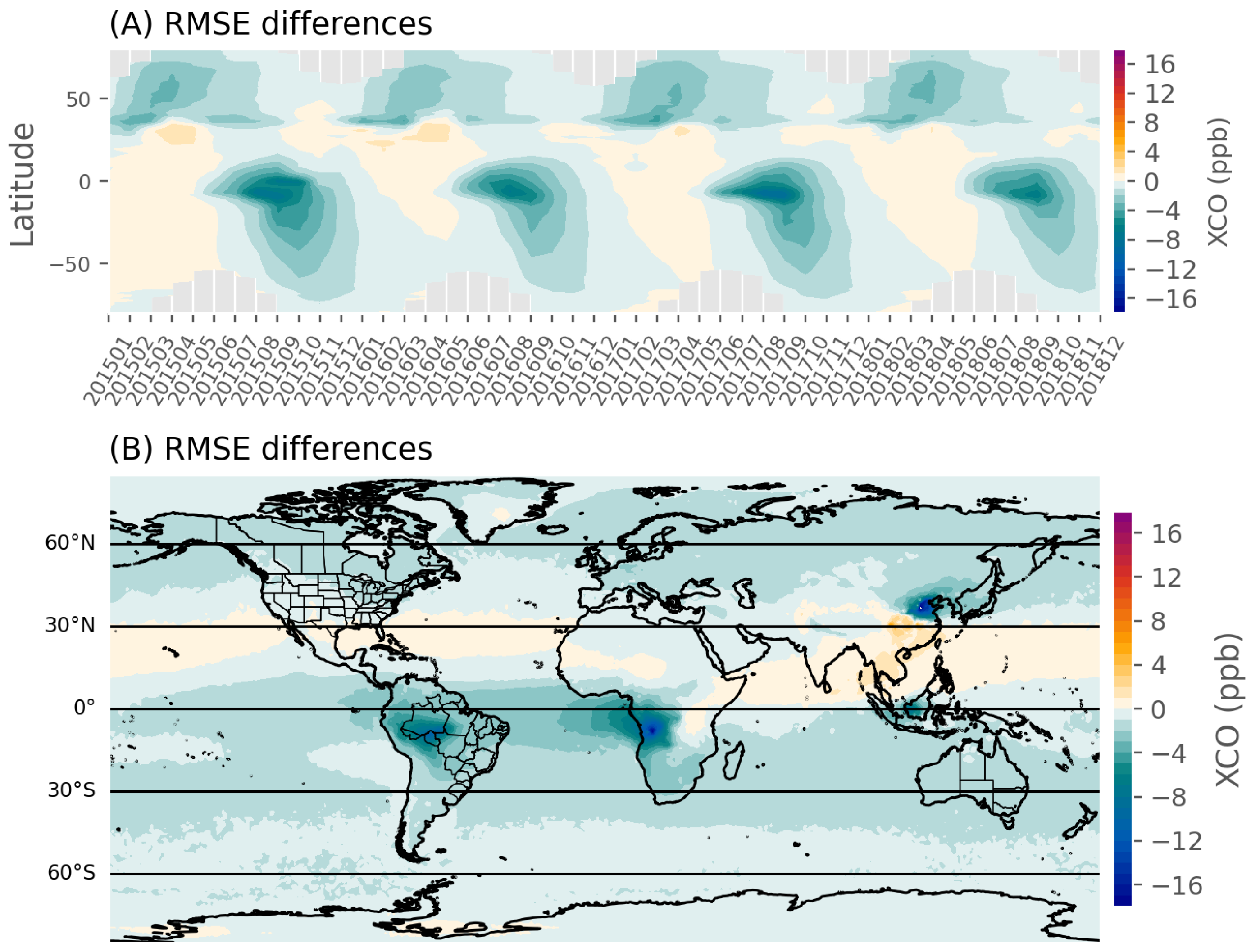
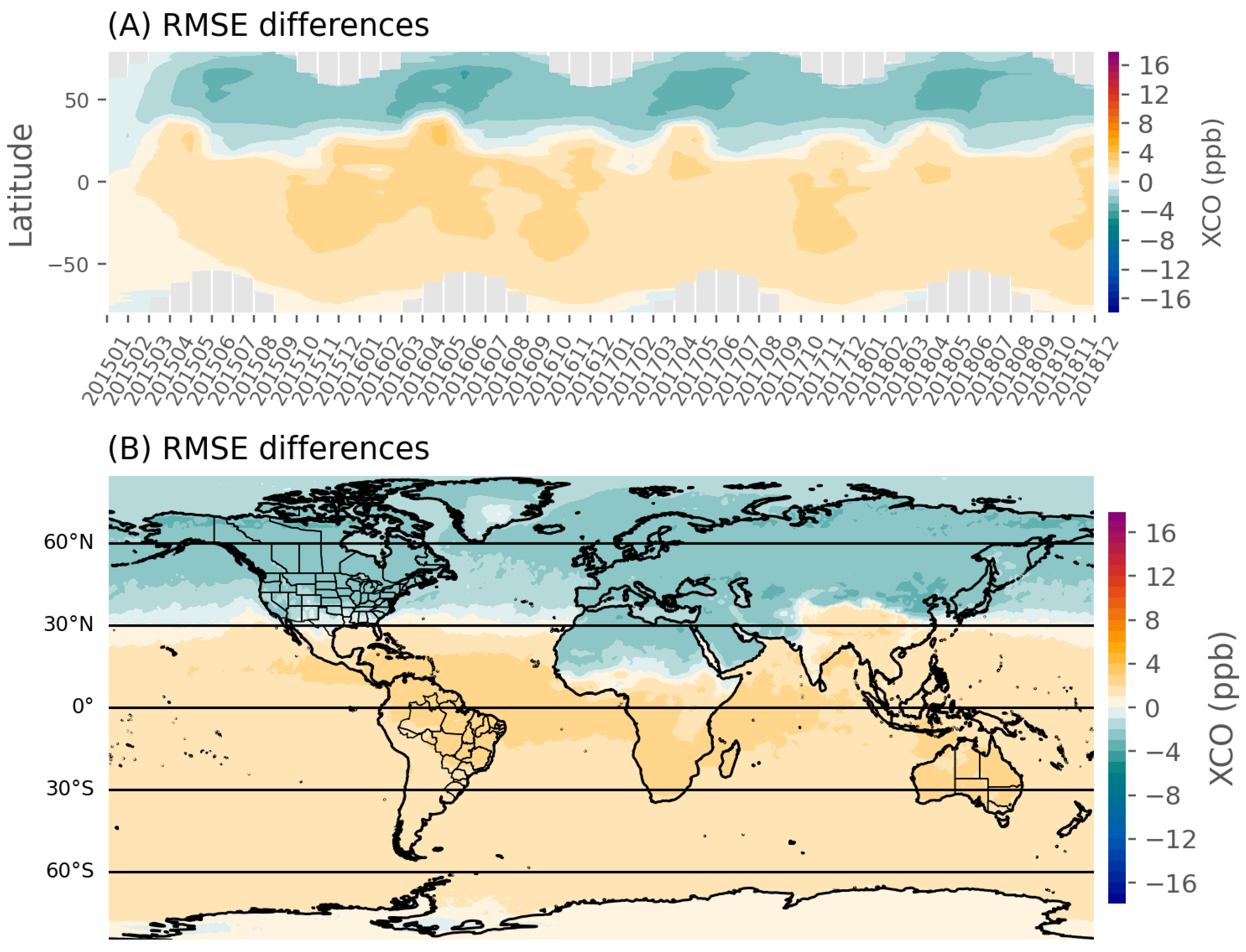
3. CO Assimilation Results

Figure 1 shows the time series of the bias for the Control-DA and the MOPITT-DA against the MOPITT column-average dry-air mole fraction of CO (XCO). The Control-DA overestimates MOPITT XCO by around 10 ppb or 13% in the tropics and underestimates MOPITT XCO in the northern hemisphere extratropics by 20 ppb or 23%, with only small changes over time.

It suggests systematic differences in the drivers of XCO and their errors between the tropics and the northern extratropics. As expected, in the MOPITT-DA, the bias evolves from the bias of the initial ensemble to the bias of the analysis model states, with residual 6 h forecast errors of less than 10 ppb towards the end of the month. With the adjustments of the emissions and no constraints on OH, it suggests that transport error or an OH overestimation is responsible for the negative bias during the 6 h forecast. With the bias becoming stationary for the last 10 days, we will be assuming a spinup period of 15 days.

We show the 15-day MOPITT XCO average in Figure 2. Most of the large XCO enhancements (top panel) are caused by fires, such as in the western United States, Eastern Europe, Siberia in Amazonia, and the Indonesian peninsula, with the largest values found over southern tropical Africa. Large XCO values from mainly anthropogenic sources are also found in East Asia. As a result, the background XCO is large over the Pacific and Atlantic continental outflow north of 30$°$N. Large values are also found in the tropical Atlantic, Pacific, and Indian oceans, following easterly outflows at the equator from mainly biomass burning sources. A strong underestimation is found over the extratopical northern hemisphere, with slightly larger biases over the continental areas (middle panel). The only exception is found over Northern and Eastern India and close to the fires in Siberia, with slightly positive biases.

The background CO is better reproduced on average in the tropics and in the southern hemisphere. However, positive biases, larger than a 20 ppb overestimation of the columns, are found over the biomass burning regions in South America, tropical Africa, and the Indonesian Peninsula. The overestimation extends far from the sources along the equator. As expected from the assimilation, the MOPITT-DA shows considerably reduced biases (bottom panel). The errors remain within the 10 ppb range, which is reasonable considering the observation errors (∼10%) and other sources of model error stemming from transport and chemistry representation. Aside from the equatorial fire plumes, XCO tends to be underestimated. We further evaluate the MOPITT assimilation results by comparing them with the NDACC FTIR observations. Figure 3 shows the improvements in the tropospheric wVMR CO columns as measured by 15 NDACC sites for 15 August 2015 to 31 August 2015. The mean absolute bias is reduced from around 19 ppb to 11 ppb and the correlation coefficient increases from 0.74 to 0.94.

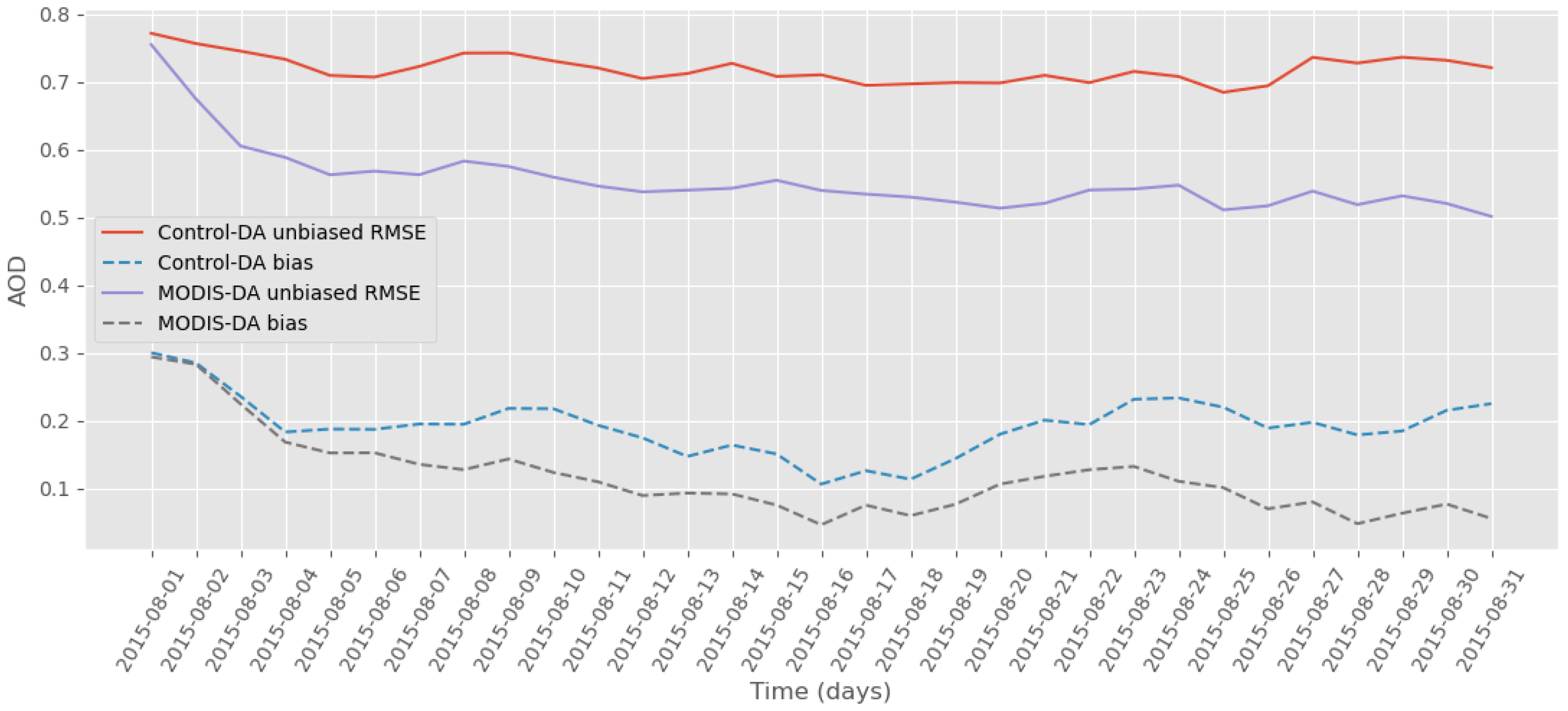
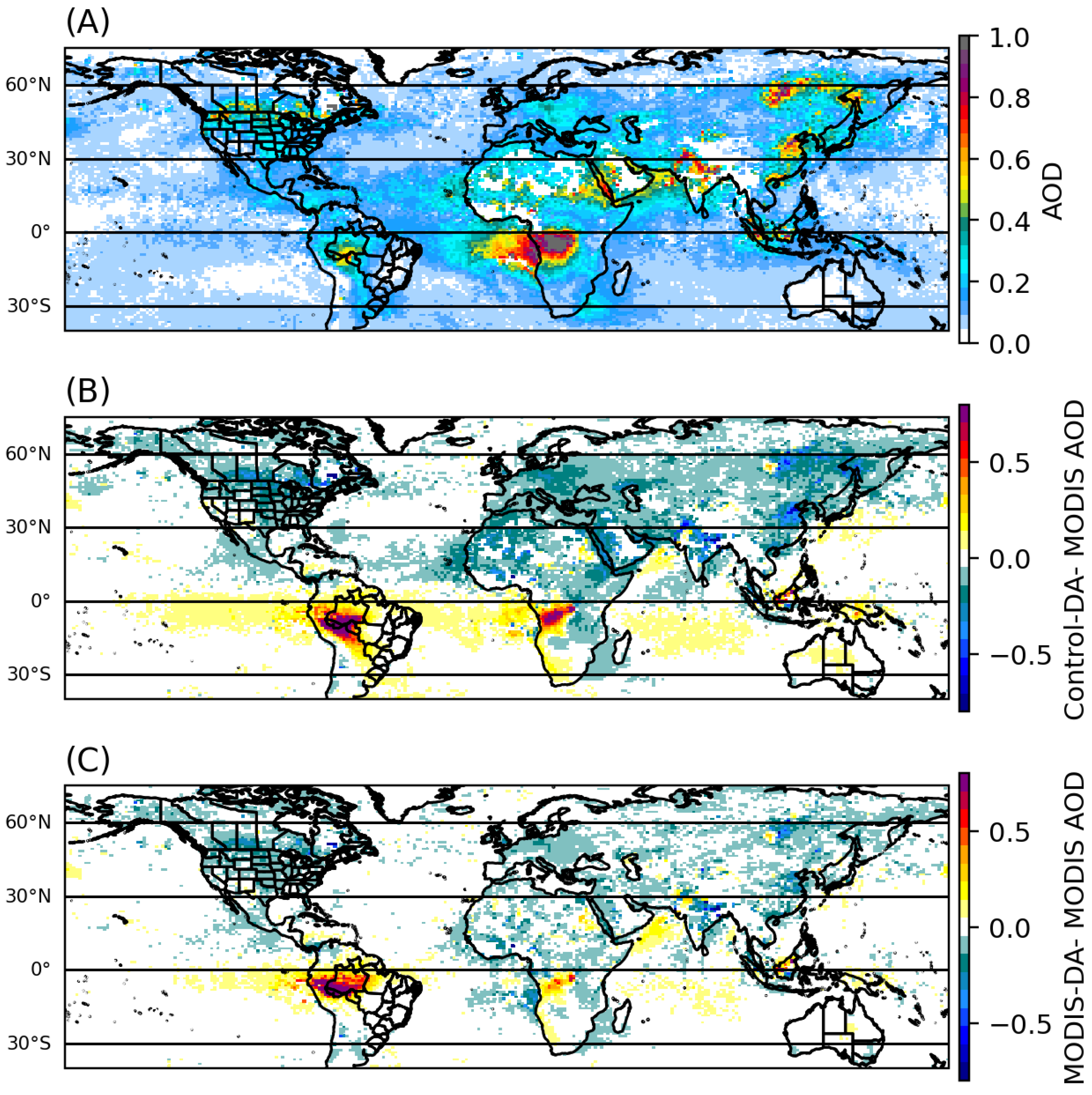
4. Aerosol Optical Depth (AOD) Assimilation Results

The verification of the assimilation experiment is first performed by comparing the 6 h forecast statistics for the MODIS-DA and Control-DA simulations against the MODIS AOD observations. Figure 4 displays the global and daily biases and unbiased root mean square error (RMSE) for both simulations. For the Control-DA, the error remains stable for the entire month, with an unbiased RMSE above 0.7 and a positive bias of around 0.2. The MODIS-DA unbiased RMSE rapidly decreases in the first few days and stabilizes between 0.5 and 0.6, which corresponds to an error reduction of 30%.

Figure 5 illustrates the spatial distribution of the assimilated MODIS AOD observations and the bias for the Control-DA and the MODIS-DA averaged over the entire month of August 2015. The largest AODs result from the fires in the tropics and over Siberia, and from anthropogenic sources in Northeast China and over the Indo-Gangetic Plains, in line with previous studies [112]. As for CO, the AOD values over the fire sources and outflows are overestimated, with the largest biases over South America (top panel). The Control-DA underestimates the AOD over most of the northern hemisphere, mostly over land, including the dust source over the Sahara Desert. The assimilation corrects the forecast AOD, with much smaller biases in most places but South America. The magnitude and the spatial extent of the AOD biases are reduced over southern regions and downwind.

The AOD biases are similar to CO and are thus indicating a strong signal from similar emission sources and potentially transport. However, the processes responsible for the total AOD are different than for CO, reflecting a larger diversity of sources such as sea salt, dust, and sulfate aerosols, and physical and chemical processes including secondary organic aerosol formation. Figure 6 shows the differences in AOD speciation between the MODIS-DA and the Control-DA. It allows the identification of which species are changed following the assimilation and which ones are potentially the dominant sources of errors. The patterns for the primary and secondary organic aerosols and black carbon are similar to the CO bias patterns as well, with an overestimation of tropical fire and an underestimation of fires in the mid-latitudes. The extent of the correction indicates that the emissions are not the only source of errors. The sulfates were increased following the assimilation, with the largest increase over the Arabian Peninsula, Northeast China, and South America. The large sulfate aerosol abundance is responsible for the residual biases over South America and indicates shortcomings in the assimilation, likely due to model errors such as convection. The assimilation also indicates errors in the transport of dust aerosols, with decreases over some source regions such as Eastern Sahara and Australia, but increases downwind over Northwest Africa and the Northern Tropical Atlantic Ocean. The sea salt aerosols were slightly overestimated in the Control-DA simulation.

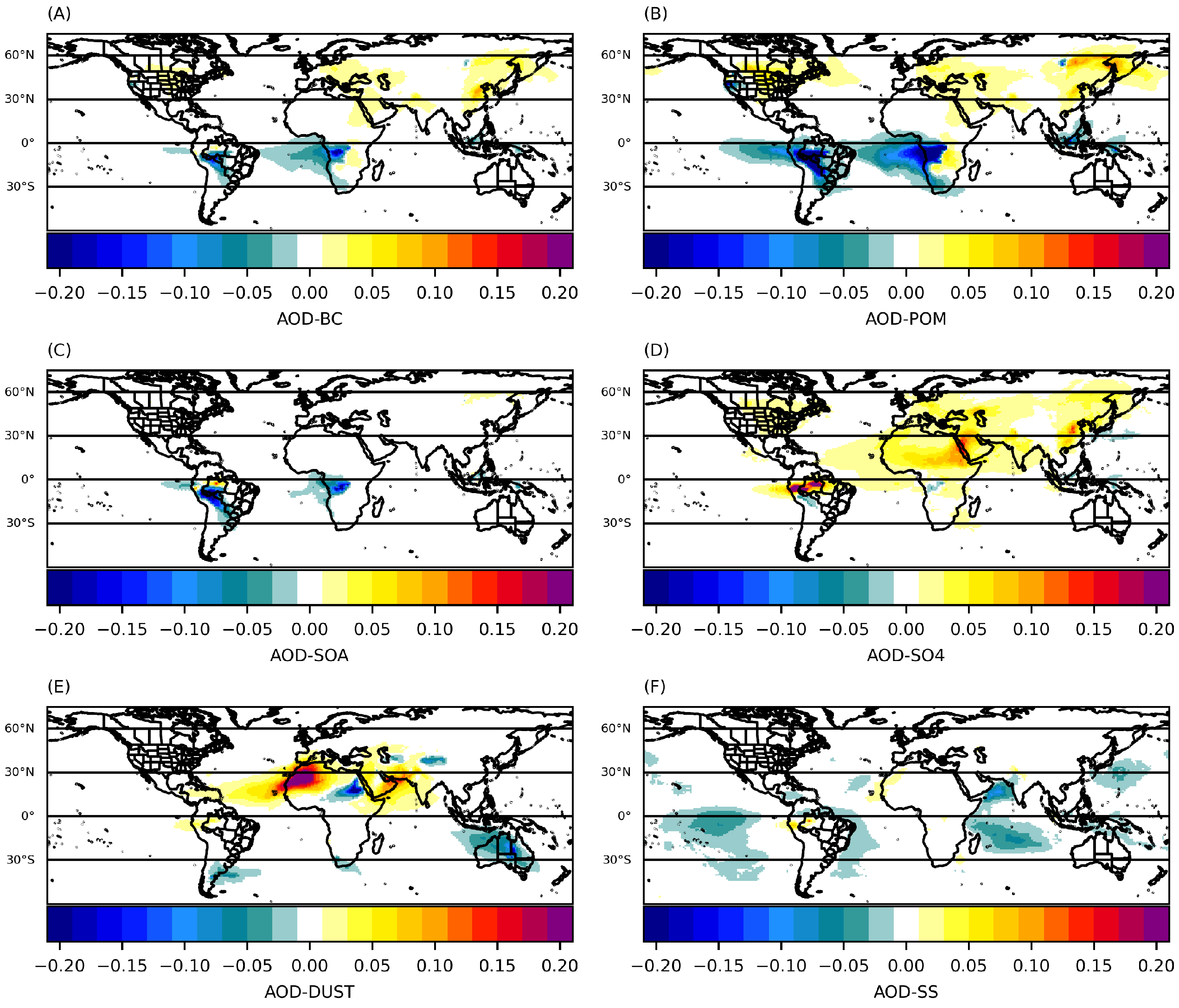
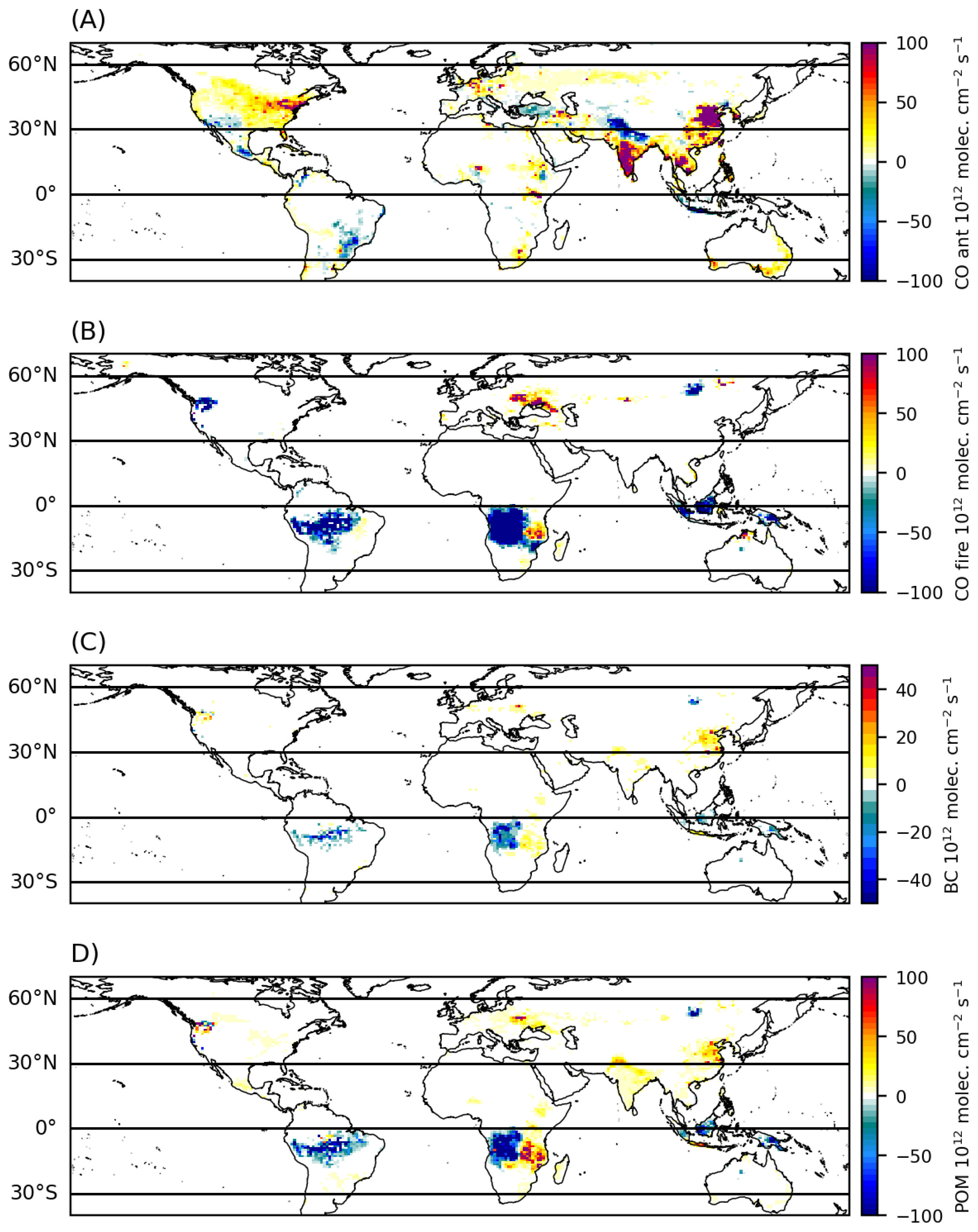
5. Impacts of Posterior Emissions and Chemistry

We average the posterior emissions across the ensemble and for the entire month to smooth out the ensemble noise. Figure 7 displays the differences for the absolute fluxes obtained from the inversions. As for the concentration, the patterns of the emission increments are strikingly similar between the MOPITT-CO and the MODIS-AOD inversions. This confirms the systematic uncertainties, resulting from a combination of mostly emissions and potentially transport contributions of the model errors, since these two factors are common for both CO and AOD. The anthropogenic CO covers larger areas—for instance, over the United States and Eurasia. Strong positive increments are found over Northeast China and South Asia, while negative increments are found over Northern India. The main difference between CO and POM (and BC) resides in Northern India, where the POM (and BC) emissions are increased, but anthropogenic CO emissions are decreased. The differences seen in India could be a misattribution of the FINN fire CO overestimation to anthropogenic sources. Elsewhere, the sign of the fire emission increments is consistent with aerosol emission increments for the AOD and CO inversions, with decreases in South America, the western side of southern tropical Africa, Indonesia, the US, Canada’s Pacific Northwest, and Siberia and an increase in the fires in Russia.

Table 3. Total emissions for 2015. In addition to our prior CAMS-GLOB-ANT_v5.1 (CAMS v5.1), we also show the Community Emissions Data System (CEDSv2) [81] and Hemispheric Transport of Air Pollution (HTAPv3) [113]. We also compare with the Quick-Fire Emissions Dataset or QFED for fire emissions [115]. For both BC and OC, all simulations include the same FINN2.5 fire emissions.

CO${}_{\mathit{ant}}$ (Tg a${}^{-1}$)	CAMS v5.1	Posterior	CEDSv2	HTAPv3
Global	578.1	607.65	558.63	535.17
China	127.18	146.87	160.39	164.73
India	68.24	68.5	63.53	70.13
USA	46.25	48.82	40.42	37.13
Nigeria	22.76	23.04	12.99	21.44
Brazil	28.48	28.48	14.63	21.66
Russia	9.16	9.27	8.0	8.5
CO${}_{fire}$ (Tg a${}^{-1}$)	FINN2.5	Posterior	QFED
Global	776.88	724.78	344.65
China	17.34	17.37	7.4
India	17.26	17.26	2.94
USA	20.39	19.77	16.58
Nigeria	3.61	3.61	2.1
Brazil	112.73	97.96	34.15
Russia	36.75	36.53	24.74
BC${}_{ant+fire}$ (Tg a${}^{-1}$)	CAMSv5.1	Posterior	CEDSv2	HTAPv3
Global	10.23	11.5	11.47	11.61
China	1.37	2.18	1.45	1.84
India	0.88	1.05	1.01	1.0
USA	0.34	0.43	0.32	0.38
Nigeria	0.23	0.24	0.2	0.23
Brazil	0.94	0.78	0.87	0.92
Russia	0.35	0.37	0.48	0.36
OC${}_{ant+fire}$ (Tg a${}^{-1}$)	CAMS v5.1	Posterior	CEDSv2	HTAPv3
Global	70.72	71.17	73.49	72.15
China	4.71	6.99	3.94	5.14
India	3.63	4.19	4.67	4.2
USA	2.19	2.38	2.23	2.61
Nigeria	1.13	1.17	1.06	1.1
Brazil	8.69	6.38	8.43	8.67
Russia	2.81	2.91	3.05	2.82

shows various emission estimates at the global scale and for large countries in 2015. It shows overall consistency at the global and annual scale between the various estimates. The posterior anthropogenic CO emissions are increased compared to the CAMS-GLOB-ANT_v5.1. The total yearly Chinese emissions for 2015 are 127 Tg a${}^{-1}$ for CAMS-GLOB-ANT_v5.1 (prior) and in 147 Tg a${}^{-1}$ in our posterior, 160 Tg a${}^{-1}$ for CEDSv2, and 165 Tg a${}^{-1}$ for HTAPv3. Our top-down emission estimate is around 16% higher than the CAMS-GLOB-ANT_v5.1, but remains lower than version 3 of the Hemispheric Transport of Air Pollution (HTAPv3) [113] and the Community Emissions Data System (CEDSv2) [81]. It is also lower than the value of 162 Tg a${}^{-1}$ in 2015 reported in Li et al. [114] from the Multi-Resolution Emission Inventory for China (MEIC v1.2) This suggests that the CAMS-GLOB-ANT_v5.1 inventory underestimates anthropogenic CO emissions for China in 2015. The CAMS-GLOB-ANT_v5.1 and the posterior and HTAPv3 show good correspondence over Nigeria and Brazil, where CEDSv2 is much lower.

As already noted in Wiedinmyer et al. [83], the FINN2.5 emissions estimate much larger emissions, 777 Tg a${}^{-1}$ in 2015, when QFED is 345 Tg a${}^{-1}$. This confirms our reduction estimated from top-down assimilation but our totals remains much higher than QFED. The comparison with QFED also indicates much larger FINN emissions in China and India. A longer assimilation run is needed to provide an accurate estimate of biomass burning emissions for fires.

For aerosols, only anthropogenic emissions inventories are shown. The slight increase in emissions for both BC and OC brings the posterior closer to HTAPv3 and CEDSv2 estimates at the global scale and for India and Russia. As opposed to CO, the higher emissions in China and India and for BC and OC are not supported by the other inventories. The comparison with QFED fire emissions suggests that this could be due to an overestimation of FINN fire emissions in India and China.

As summarized in Table 1, we performed a series of forward simulations to assess the impact of posterior emissions and of a change in the main tropospheric OH source. The CAM-chem simulations were initialized from the same initial conditions on 1 January 2015 and run until 1 January 2019. The resulting relative emissions changes were applied to the original fluxes, i.e., the daily FINN2.2 emissions, and by sector for the monthly CAMS-GLOB-ANT_v5.1. Assuming that the errors were stationary, we applied these increments over all time steps for both emission sources.

In order to verify the impact of sustained emissions changes across all time steps, we performed deterministic simulations with the posterior CO emissions (CAM-chem-post) and with the posterior BC and POM emissions (CAM-chem-post-aer). Since JO(${}^1$D) plays an important role in OH formation (e.g., [54,116]), we performed another simulation where we arbitrarily reduced the ozone photolysis of JO(${}^1$D) by 10% globally (CAM-chem-O1D simulation). This simulation was designed to cut the OH production from its primary source, which was JO(${}^1$D), and the dominant source in remote environments where ATom measurements are made.

Figure 8, Figure 9 and Figure 10 contrast the results with respect to the control for CAM-chem-post (updated CO emissions), CAM-chem-O1D (reduction in JO(${}^1$D)), and aerosol emissions (CAM-chem-post-aer), respectively. It shows the differences in RMSE compared to monthly MODIS AOD and MOPITT CO observations. The strongest signals comes from East Asian emissions and tropical fires, which show large-scale improvements close to the emission hotspots, with RMSE reductions in XCO by up to 15 ppb. The reduction in RMSE can propagate through continental outflows at large scale and far from the sources. Large biases in tropical fire estimates propagate through the entire southern hemisphere [117]. On average, the XCO improvement can be seen over the entire southern hemisphere. This is driven by the bias reduction during the fire season, from August to October. The bias reduction then propagates through the lower latitudes, spreading over the whole southern hemisphere by December. The performance of the updated simulation is degraded with respect to the reference in the equatorial latitudes of the northern hemisphere, where the bias has the opposite sign to the emission correction. In particular, there have been no constraints on the fire sources in Southeast Asia and an increase in anthropogenic emissions. During the fire season in boreal spring, the FINN2.2 emissions are overestimated and the posterior simulation’s bias is increased, impacting the Pacific outflow. This result is consistent with the Southeast Asian overestimation reported in Wiedinmyer et al. [83].

The simulated tropospheric and global CH${}_4$ lifetimes for 2015 are not changed between the two CO emissions, 7.9 years, which is 1.5 years too short. The reduction in fire CO emissions might compensate for the increase in anthropogenic emissions. The lack of differences between the two simulations could be explained by the fact that an increase in CO emissions could lead to O${}_3$ production [52], which, in turn, produces OH, especially in boreal summer. The CH${}_4$ lifetime increases to 8.3 years in the CAM-chem-O1D simulation.

Figure 9 illustrates this pattern, with a clear reduction in RMSE in the northern mid-latitudes and an increase in RMSE in the tropics and in the southern hemisphere. While the dipole can be explained by the biases in emissions that we identified earlier, this global decrease in OH has a strong impact on XCO and confirms the important role of modeled OH on the CO systematic errors. Beyond the role of emissions, the XCO error sensitivity to OH does not show a seasonal pattern.

It emphasizes the role of the ongoing metrics of inter-hemispheric parity as playing a strong role in forward simulations. Indeed, the simulated N/S ratio is 1.42 in 2015 and is only slightly reduced to 1.41 in the CAM-chem-post simulation. While a JO(${}^1$D) change should lead to a linear and proportional reduction in primary OH production of 10% [116], we only found a 4.5% reduction in air mass weighted global and annual (2015) tropospheric OH. This suggests strong secondary OH production, which seems to explain the lack of sensitivity to CO emission changes. It would play a role in inverse modeling systems that do not correct for initial conditions in the case of interactive chemistry or with a wrongly prescribed OH otherwise.

The impacts on aerosols are more localized because of the shorter lifetime, with improvements close to the source, especially over China, the Congo Basin, and over the Amazon (Figure 10). The improvements are better than for CO over India and the degradation is not as pronounced in Southeast Asia and the Pacific Ocean. The changes in the African tropical outflow are a contrast between larger improvements and degradation overall. These are the result of the convolution of opposing bias between emissions and transport. There is mostly a reduction in emissions in the southern (northern) part of the outflow around 15$°$S (0$°$S), where the AODs are underestimated (overestimated), increasing (decreasing) the relative errors, respectively.

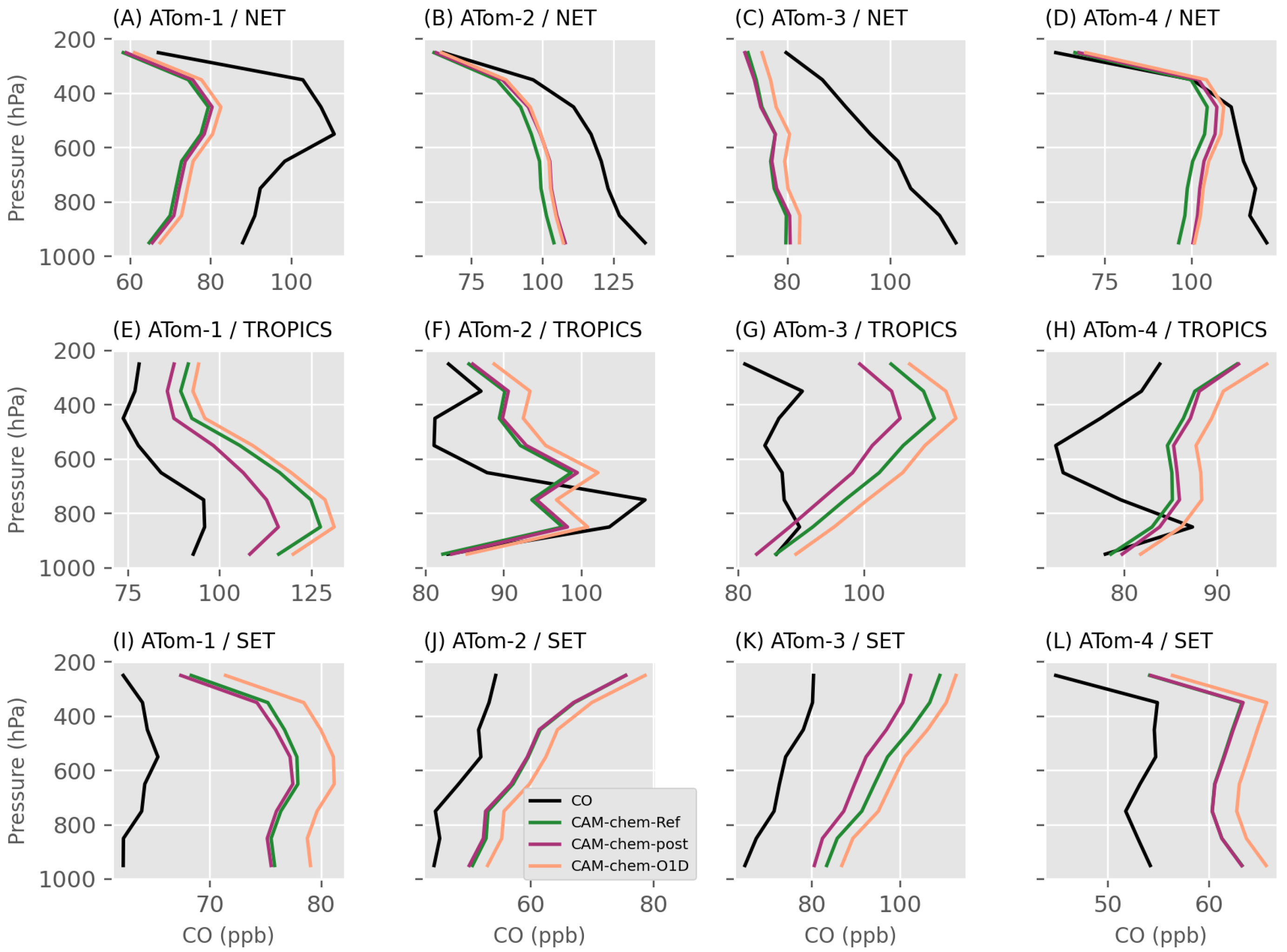
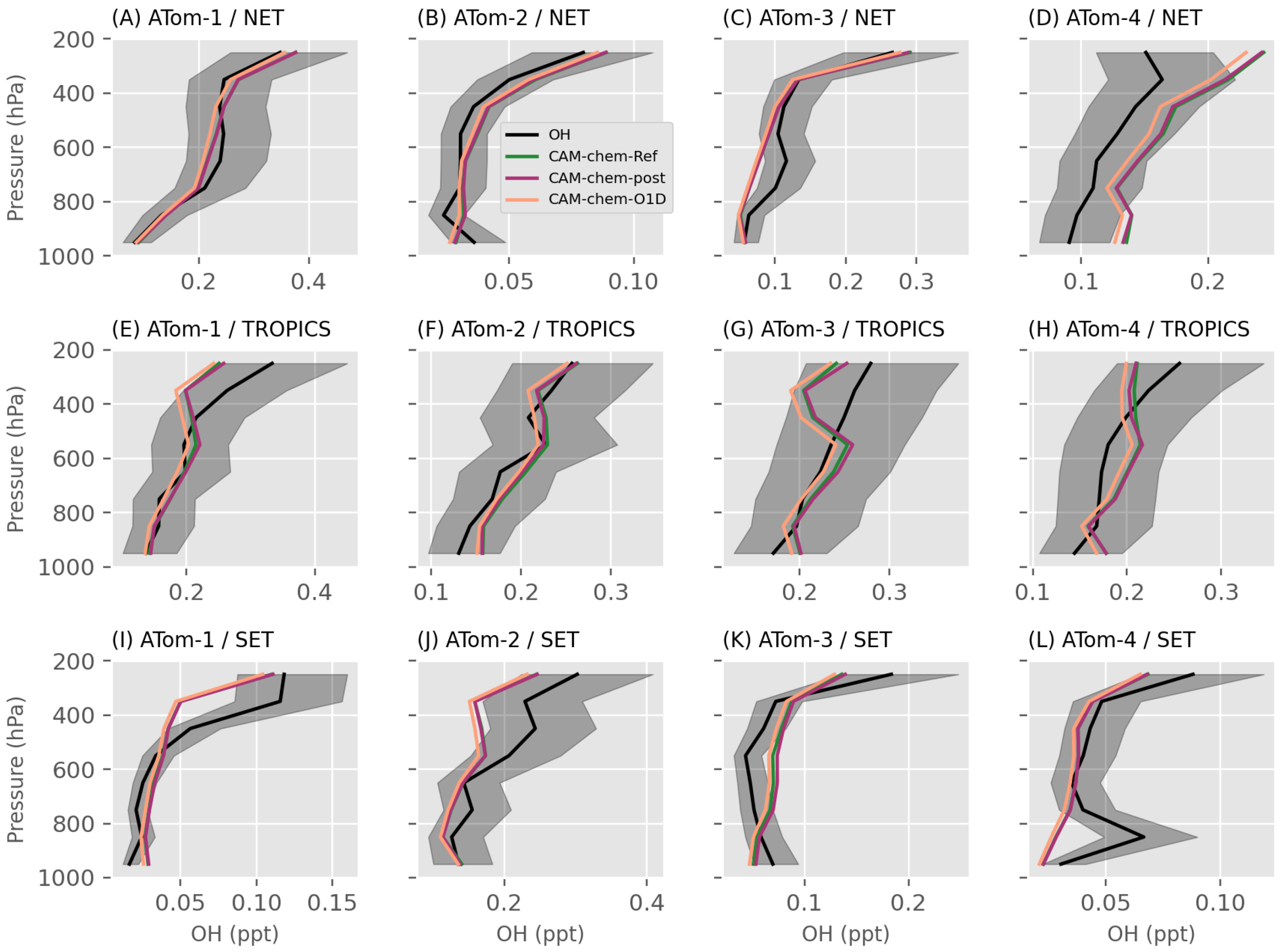
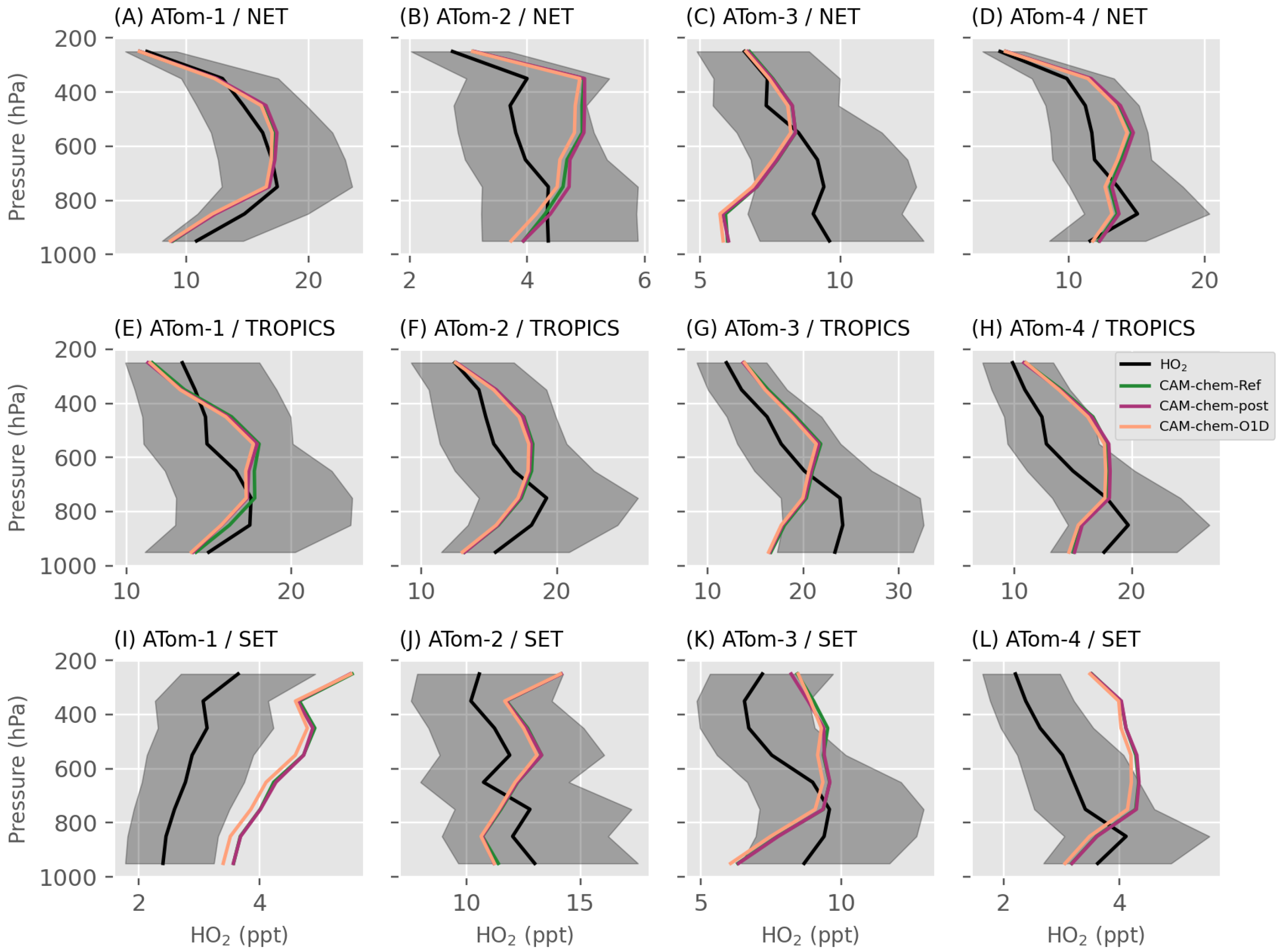
6. Evaluation against NASA ATom

Figure 11 shows the average CO over latitudinal bands for the four ATom experiments. The CO underestimation in the remote atmosphere of the northern hemisphere is actually found for all seasons and is the largest for ATom-3 in the fall 2017. The increase in emissions leads to a modest improvement in winter (ATom-2) and spring (ATom-4) and is not particularly noticeable in summer (ATom-1) or fall (ATom-3). In the tropics, the challenge is in representing the biomass burning enhancement. Both simulations tend to overestimate CO for all seasons. Following the reduction in fire emissions, the bias is reduced for ATom-1 and ATom-3, corresponding to the fire season in southern tropical Africa and South America. The profile for ATom-3 indicates the large convective transport of CO to the upper troposphere, a feature not present in the observation. The least that we can say is that the sensitivity to a change in emissions is minuscule in the remote atmosphere. As for the column, it suggests that the background concentration, because of the chemical loss on one hand and the chemical production on the other hand, is driven by chemistry.

The impact on CO is at least as large as the emission change in most cases. In the southern hemisphere, differences of up to 5 ppb over the entire profile are found for ATom-1 and Atom-3, which correspond to austral winter and spring.

Figure 12 shows the vertical OH observations and simulations for both hemispheres. The model simulations and observations show good agreement overall, especially in the northern hemisphere. The simulations tend to overestimate OH in the upper troposphere of the southern hemisphere. There is an apparent bias for ATom-2 and ATom-4 with overestimation for the entire profiles, which could explain some of the CO bias observed in boreal winter and spring. As expected, the reduction in JO(${}^1$D) reduces OH for all ATom in both hemispheres. HO${}_2$ (Figure 13) is mostly overestimated in the upper troposphere for both hemispheres. This indicates that the HO${}_x$ are overestimated in a fairly consistent manner. Since HO${}_2$ tends to be slightly underestimated in the lower troposphere, some CO direct or indirect sources may still be missing, which would reduce OH and increase HO${}_2$, although we cannot rule out the effect of nitrogen and other oxidants’ chemistry.

7. Discussion

Other studies have focused on directly quantifying urban CO emissions from model simulations and satellite data [118,119,120]. With the increased spatial resolution from more recent satellites, such as the Tropospheric Monitoring Instrument (TROPOMI), emissions can be detected at smaller, i.e., sub-city, scales [121] and by sector, such as facility-level industrial sources [122]. Recently, Sun [123] extended such a framework to estimate emissions over the entire contiguous United States (CONUS) on a 0.04$°$ mesh. Recent studies have investigated the use of machine learning algorithms to estimate high-resolution near-surface CO concentrations by combining surface observations and MOPITT observations [124], and directly from satellite radiances augmented by a deep forest (DF) model [125]. However, Tang et al. [126] raised the question of the spatial and temporal representativeness of satellites compared to the surface observations using data assimilation over China. Emission estimates from the various approaches must be compared in future studies.

The impact of meteorological uncertainties through dynamical and physical processes are taken into account in our chemical ensemble data assimilation system. However, biases in the planetary boundary layer height and deep convection are likely to play an important role in predicting the concentrations of gas-phase and aerosol atmospheric constituents. Examples of the comparison of simulated planetary boundary layer heights with LiDAR observations indicate daytime overestimation, implying the excessive dilution of emission fluxes (e.g., [127,128]). The boundary layer mixing is also important in chemistry and can have impacts on wet and dry deposition, impacting global tropospheric OH and O${}_3$ budgets [129]. Refining the grid mesh to a higher resolution should help in representing smaller-scale topography gradients, while increasing the vertical resolution will improve the representation of parameters relevant to vertical transport. An increase in spatial resolution will help to alleviate representation errors due to differences in the urban CO and synoptic CO background [126]. We will further investigate these issues with currently developed modeling tools such as the Multi-Scale Infrastructure for Chemistry and Aerosols (MUSICA) [130].

8. Conclusions

The current CESM2.2/CAM-chem model overestimates OH in the northern hemisphere, leading to a short CH${}_4$ lifetime of 7.9 years. Conversely, CO tends to be overestimated in the southern hemisphere and over the tropics. This is illustrated by a northern hemisphere to southern hemisphere (N/S) ratio of 1.42. However, the optimization of the CO initial conditions with data assimilation mitigates the OH- and transport-induced CO biases during the emissions update. The emissions update allows for good forecast performance over the source regions, as opposed to reanalyses with only state assimilation (e.g., [45]).

The assimilation of MODIS AOD and MOPITT CO led to similar posterior emissions increments, indicative of biases stemming from the inventories FINN2.2 and CAMS-GLOB-ANT_v5.1 for both organic aerosols, black carbon, and CO. The FINN2.2 emissions are overestimated in the tropics for both CO and aerosols, and this bias has an impact in India and China. Overall, only India is a large source area, where CO from CAMS-GLOB-ANT_v5.1 is overestimated in the Indo-Gangetic Plain, while aerosols are underestimated. The comparison with QFED fire emissions as well as CEDSv2 and HTAPv3 indicates that this could be due to an overestimation of FINN2.2 fire emissions in India. The posterior emissions are well within the range of the bottom-up inventory in China, the top anthropogenic CO emitter. For 2015, our total annual emissions for China are 147 Tg a${}^{-1}$, between our prior, the CAMS-GLOB-ANT_v5.1 (127 Tg a${}^{-1}$), and both CEDSv2 (160 Tg a${}^{-1}$) and HTAPv3 (165 Tg a${}^{-1}$). We recommend looking at various emission estimates, including top-down, when assessing health impacts, as done in, e.g., [131].

We applied the relative posterior emission increments, which led to the improvement of the deterministic model simulation close to the source region, and performed a simulation with a reduction in the OH primary source by 10%. Since the fire emissions play an important role in the southern hemisphere and over the tropics and impact CO at remote locations, reducing the emissions bias improved the simulated CO and AOD over large areas of these regions. Our sensitivity experiments for the year 2015 to 2018 suggest that OH is the main driver of the commonly found CO underestimation in the northern hemisphere. The comparison with NASA ATom observations indicates that the remaining biases in remote regions are driven by transport and chemistry, as well as the long-range transport of emissions, which should be considered when performing inversions. Finally, in the case of emissions, flux inversion can remediate many systematic errors. For instance, the reduction in the FINN fire emissions using observations from 2015 improved the simulations for the entire period of 2015 to 2019 close to the sources and in the outflow, for both CO and aerosols. The biases in CO are reduced in the tropics in comparison with ATom in August 2016 and during ATom-3 in October 2017, when and where the fire plumes were sampled over the Atlantic and Pacific basins. Similarly, a reduction in OH consistently improves CO in the northern mid-latitudes.

References

1. Talagrand, O. Assimilation of Observations, an Introduction. J. Meteorol. Soc. Jpn. 1997, 75, 191–209. [Google Scholar] [CrossRef]
2. Kalnay, E. Atmospheric Modeling, Data Assimilation and Predictability; Cambridge University Press: Cambridge, UK, 2002. [Google Scholar] [CrossRef]
3. Lahoz, W.A.; Schneider, P. Data assimilation: Making sense of Earth Observation. Front. Environ. Sci. 2014, 2, 16. [Google Scholar] [CrossRef]
4. Bocquet, M.; Elbern, H.; Eskes, H.; Hirtl, M.; Žabkar, R.; Carmichael, G.R.; Flemming, J.; Inness, A.; Pagowski, M.; Camaño, J.L.P.; et al. Data assimilation in atmospheric chemistry models: Current status and future prospects for coupled chemistry meteorology models. Atmos. Chem. Phys. 2015, 15, 5325–5358. [Google Scholar] [CrossRef]
5. Collins, W.D.; Rasch, P.J.; Eaton, B.E.; Khattatov, B.V.; Lamarque, J.F.; Zender, C.S. Simulating aerosols using a chemical transport model with assimilation of satellite aerosol retrievals: Methodology for INDOEX. J. Geophys. Res. Atmos. 2001, 106, 7313–7336. [Google Scholar] [CrossRef]
6. Zhang, L.; Jacob, D.J.; Boersma, K.F.; Jaffe, D.A.; Olson, J.R.; Bowman, K.W.; Worden, J.R.; Thompson, A.M.; Avery, M.A.; Cohen, R.C.; et al. Transpacific transport of ozone pollution and the effect of recent Asian emission increases on air quality in North America: An integrated analysis using satellite, aircraft, ozonesonde, and surface observations. Atmos. Chem. Phys. 2008, 8, 6117–6136. [Google Scholar] [CrossRef]
7. Saide, P.E.; Kim, J.; Song, C.H.; Choi, M.; Cheng, Y.; Carmichael, G.R. Assimilation of next generation geostationary aerosol optical depth retrievals to improve air quality simulations. Geophys. Res. Lett. 2014, 41, 9188–9196. [Google Scholar] [CrossRef]
8. Benedetti, A.; Morcrette, J.J.; Boucher, O.; Dethof, A.; Engelen, R.J.; Fisher, M.; Flentje, H.; Huneeus, N.; Jones, L.; Kaiser, J.W.; et al. Aerosol analysis and forecast in the European Centre for Medium-Range Weather Forecasts Integrated Forecast System: 2. Data assimilation. J. Geophys. Res. 2009, 114. [Google Scholar] [CrossRef]
9. Schutgens, N.A.J.; Miyoshi, T.; Takemura, T.; Nakajima, T. Applying an ensemble Kalman filter to the assimilation of AERONET observations in a global aerosol transport model. Atmos. Chem. Phys. 2010, 10, 2561–2576. [Google Scholar] [CrossRef]
10. Pagowski, M.; Grell, G.A.; McKeen, S.A.; Peckham, S.E.; Devenyi, D. Three-dimensional variational data assimilation of ozone and fine particulate matter observations: Some results using the Weather Research and Forecasting-Chemistry model and Grid-point Statistical Interpolation. Q. J. R. Meteorol. Soc. 2010, 136, 2013–2024. [Google Scholar] [CrossRef]
11. Schwartz, C.S.; Liu, Z.; Lin, H.C.; McKeen, S.A. Simultaneous three-dimensional variational assimilation of surface fine particulate matter and MODIS aerosol optical depth. J. Geophys. Res. Atmos. 2012, 117. [Google Scholar] [CrossRef]
12. Pagowski, M.; Grell, G.A. Experiments with the assimilation of fine aerosols using an ensemble Kalman filter. J. Geophys. Res. Atmos. 2012, 117. [Google Scholar] [CrossRef]
13. Schwartz, C.S.; Liu, Z.; Lin, H.C.; Cetola, J.D. Assimilating aerosol observations with a “hybrid” variational-ensemble data assimilation system. J. Geophys. Res. Atmos. 2014, 119, 4043–4069. [Google Scholar] [CrossRef]
14. Rubin, J.I.; Reid, J.S.; Hansen, J.A.; Anderson, J.L.; Collins, N.; Hoar, T.J.; Hogan, T.; Lynch, P.; McLay, J.; Reynolds, C.A.; et al. Development of the Ensemble Navy Aerosol Analysis Prediction System (ENAAPS) and its application of the Data Assimilation Research Testbed (DART) in support of aerosol forecasting. Atmos. Chem. Phys. 2016, 16, 3927–3951. [Google Scholar] [CrossRef]
15. Rubin, J.I.; Reid, J.S.; Hansen, J.A.; Anderson, J.L.; Holben, B.N.; Xian, P.; Westphal, D.L.; Zhang, J. Assimilation of AERONET and MODIS AOT observations using variational and ensemble data assimilation methods and its impact on aerosol forecasting skill. J. Geophys. Res. Atmos. 2017, 122, 4967–4992. [Google Scholar] [CrossRef]
16. Kumar, S.V.; Mocko, D.M.; Wang, S.; Peters-Lidard, C.D.; Borak, J. Assimilation of Remotely Sensed Leaf Area Index into the Noah-MP Land Surface Model: Impacts on Water and Carbon Fluxes and States over the Continental United States. J. Hydrometeorol. 2019, 20, 1359–1377. [Google Scholar] [CrossRef]
17. Sandu, A.; Chai, T. Chemical Data Assimilation-An Overview. Atmosphere 2011, 2, 426–463. [Google Scholar] [CrossRef]
18. Elbern, H.; Strunk, A.; Schmidt, H.; Talagrand, O. Emission rate and chemical state estimation by 4-dimensional variational inversion. Atmos. Chem. Phys. 2007, 7, 3749–3769. [Google Scholar] [CrossRef]
19. Miyazaki, K.; Eskes, H.J.; Sudo, K.; Takigawa, M.; van Weele, M.; Boersma, K.F. Simultaneous assimilation of satellite NO2, O3, CO, and HNO3 data for the analysis of tropospheric chemical composition and emissions. Atmos. Chem. Phys. 2012, 12, 9545–9579. [Google Scholar] [CrossRef]
20. Peng, Z.; Liu, Z.; Chen, D.; Ban, J. Improving PM2.5 forecast over China by the joint adjustment of initial conditions and source emissions with an ensemble Kalman filter. Atmos. Chem. Phys. 2017, 17, 4837–4855. [Google Scholar] [CrossRef]
21. Peng, Z.; Lei, L.; Liu, Z.; Sun, J.; Ding, A.; Ban, J.; Chen, D.; Kou, X.; Chu, K. The impact of multi-species surface chemical observation assimilation on air quality forecasts in China. Atmos. Chem. Phys. 2018, 18, 17387–17404. [Google Scholar] [CrossRef]
22. Miyazaki, K.; Bowman, K.; Sekiya, T.; Eskes, H.; Boersma, F.; Worden, H.; Livesey, N.; Payne, V.H.; Sudo, K.; Kanaya, Y.; et al. Updated tropospheric chemistry reanalysis and emission estimates, TCR-2, for 2005–2018. Earth Syst. Sci. Data 2020, 12, 2223–2259. [Google Scholar] [CrossRef]
23. Ma, C.; Wang, T.; Mizzi, A.P.; Anderson, J.L.; Zhuang, B.; Xie, M.; Wu, R. Multiconstituent Data Assimilation With WRF-Chem/DART: Potential for Adjusting Anthropogenic Emissions and Improving Air Quality Forecasts Over Eastern China. J. Geophys. Res. Atmos. 2019, 124, 7393–7412. [Google Scholar] [CrossRef]
24. Gaubert, B.; Emmons, L.K.; Raeder, K.; Tilmes, S.; Miyazaki, K.; Arellano, A.F., Jr.; Elguindi, N.; Granier, C.; Tang, W.; Barré, J.; et al. Correcting model biases of CO in East Asia: Impact on oxidant distributions during KORUS-AQ. Atmos. Chem. Phys. 2020, 20, 14617–14647. [Google Scholar] [CrossRef] [PubMed]
25. Randles, C.A.; da Silva, A.M.; Buchard, V.; Colarco, P.R.; Darmenov, A.; Govindaraju, R.; Smirnov, A.; Holben, B.; Ferrare, R.; Hair, J.; et al. The MERRA-2 Aerosol Reanalysis, 1980 Onward. Part I: System Description and Data Assimilation Evaluation. J. Clim. 2017, 30, 6823–6850. [Google Scholar] [CrossRef] [PubMed]
26. Buchard, V.; Randles, C.A.; da Silva, A.M.; Darmenov, A.; Colarco, P.R.; Govindaraju, R.; Ferrare, R.; Hair, J.; Beyersdorf, A.J.; Ziemba, L.D.; et al. The MERRA-2 Aerosol Reanalysis, 1980 Onward. Part II: Evaluation and Case Studies. J. Clim. 2017, 30, 6851–6872. [Google Scholar] [CrossRef] [PubMed]
27. Yumimoto, K.; Tanaka, T.Y.; Oshima, N.; Maki, T. JRAero: The Japanese Reanalysis for Aerosol v1.0. Geosci. Model Dev. 2017, 10, 3225–3253. [Google Scholar] [CrossRef]
28. Inness, A.; Ades, M.; Agustí-Panareda, A.; Barré, J.; Benedictow, A.; Blechschmidt, A.M.; Dominguez, J.J.; Engelen, R.; Eskes, H.; Flemming, J.; et al. The CAMS reanalysis of atmospheric composition. Atmos. Chem. Phys. 2019, 19, 3515–3556. [Google Scholar] [CrossRef]
29. Pison, I.; Bousquet, P.; Chevallier, F.; Szopa, S.; Hauglustaine, D. Multi-species inversion of CH4, CO and H2 emissions from surface measurements. Atmos. Chem. Phys. 2009, 9, 5281–5297. [Google Scholar] [CrossRef]
30. Kopacz, M.; Jacob, D.J.; Fisher, J.A.; Logan, J.A.; Zhang, L.; Megretskaia, I.A.; Yantosca, R.M.; Singh, K.; Henze, D.K.; Burrows, J.P.; et al. Global estimates of CO sources with high resolution by adjoint inversion of multiple satellite datasets (MOPITT, AIRS, SCIAMACHY, TES). Atmos. Chem. Phys. 2010, 10, 855–876. [Google Scholar] [CrossRef]
31. Krol, M.; Peters, W.; Hooghiemstra, P.; George, M.; Clerbaux, C.; Hurtmans, D.; McInerney, D.; Sedano, F.; Bergamaschi, P.; Hajj, M.E.; et al. How much CO was emitted by the 2010 fires around Moscow? Atmos. Chem. Phys. 2013, 13, 4737–4747. [Google Scholar] [CrossRef]
32. Yin, Y.; Chevallier, F.; Ciais, P.; Broquet, G.; Fortems-Cheiney, A.; Pison, I.; Saunois, M. Decadal trends in global CO emissions as seen by MOPITT. Atmos. Chem. Phys. 2015, 15, 13433–13451. [Google Scholar] [CrossRef]
33. Jiang, Z.; Worden, J.R.; Worden, H.; Deeter, M.; Jones, D.B.A.; Arellano, A.F.; Henze, D.K. A 15-year record of CO emissions constrained by MOPITT CO observations. Atmos. Chem. Phys. 2017, 17, 4565–4583. [Google Scholar] [CrossRef]
34. Ménard, R.; Chabrillat, S.; Robichaud, A.; de Grandpré, J.; Charron, M.; Rochon, Y.; Batchelor, R.; Kallaur, A.; Reszka, M.; Kaminski, J.W. Coupled Stratospheric Chemistry–Meteorology Data Assimilation. Part I: Physical Background and Coupled Modeling Aspects. Atmosphere 2020, 11, 150. [Google Scholar] [CrossRef]
35. Miyazaki, K.; Sekiya, T.; Fu, D.; Bowman, K.W.; Kulawik, S.S.; Sudo, K.; Walker, T.; Kanaya, Y.; Takigawa, M.; Ogochi, K.; et al. Balance of Emission and Dynamical Controls on Ozone During the Korea-United States Air Quality Campaign From Multiconstituent Satellite Data Assimilation. J. Geophys. Res. Atmos. 2019, 124, 387–413. [Google Scholar] [CrossRef] [PubMed]
36. Feng, S.; Jiang, F.; Wu, Z.; Wang, H.; Ju, W.; Wang, H. CO Emissions Inferred From Surface CO Observations Over China in December 2013 and 2017. J. Geophys. Res. Atmos. 2020, 125, e2019JD031808. [Google Scholar] [CrossRef]
37. Sekiya, T.; Miyazaki, K.; Eskes, H.; Sudo, K.; Takigawa, M.; Kanaya, Y. A comparison of the impact of TROPOMI and OMI tropospheric NOx global chemical data assimilation. Atmos. Meas. Tech. 2022, 15, 1703–1728. [Google Scholar] [CrossRef]
38. Qu, Z.; Henze, D.K.; Worden, H.M.; Jiang, Z.; Gaubert, B.; Theys, N.; Wang, W. Sector-Based Top-Down Estimates of NOx, SO2, and CO Emissions in East Asia. Geophys. Res. Lett. 2022, 49, e2021GL096009. [Google Scholar] [CrossRef]
39. Ménard, R.; Gauthier, P.; Rochon, Y.; Robichaud, A.; de Grandpré, J.; Yang, Y.; Charrette, C.; Chabrillat, S. Coupled Stratospheric Chemistry–Meteorology Data Assimilation. Part II: Weak and Strong Coupling. Atmosphere 2019, 10, 798. [Google Scholar] [CrossRef]
40. Pedatella, N.M.; Liu, H.L.; Marsh, D.R.; Raeder, K.; Anderson, J.L.; Chau, J.L.; Goncharenko, L.P.; Siddiqui, T.A. Analysis and Hindcast Experiments of the 2009 Sudden Stratospheric Warming in WACCMX+DART. J. Geophys. Res. Space Phys. 2018, 123, 3131–3153. [Google Scholar] [CrossRef]
41. Flemming, J.; Benedetti, A.; Inness, A.; Engelen, R.J.; Jones, L.; Huijnen, V.; Remy, S.; Parrington, M.; Suttie, M.; Bozzo, A.; et al. The CAMS interim Reanalysis of Carbon Monoxide, Ozone and Aerosol for 2003-2015. Atmos. Chem. Phys. 2017, 17, 1945–1983. [Google Scholar] [CrossRef]
42. Huijnen, V.; Flemming, J.; Kaiser, J.W.; Inness, A.; Leitão, J.; Heil, A.; Eskes, H.J.; Schultz, M.G.; Benedetti, A.; Hadji-Lazaro, J.; et al. Hindcast experiments of tropospheric composition during the summer 2010 fires over western Russia. Atmos. Chem. Phys. 2012, 12, 4341–4364. [Google Scholar] [CrossRef]
43. Inness, A.; Baier, F.; Benedetti, A.; Bouarar, I.; Chabrillat, S.; Clark, H.; Clerbaux, C.; Coheur, P.; Engelen, R.J.; Errera, Q.; et al. The MACC reanalysis: An 8 yr data set of atmospheric composition. Atmos. Chem. Phys. 2013, 13, 4073–4109. [Google Scholar] [CrossRef]
44. Inness, A.; Blechschmidt, A.M.; Bouarar, I.; Chabrillat, S.; Crepulja, M.; Engelen, R.J.; Eskes, H.; Flemming, J.; Gaudel, A.; Hendrick, F.; et al. Data assimilation of satellite-retrieved ozone, carbon monoxide and nitrogen dioxide with ECMWF’s Composition-IFS. Atmos. Chem. Phys. 2015, 15, 5275–5303. [Google Scholar] [CrossRef]
45. Wagner, A.; Bennouna, Y.; Blechschmidt, A.M.; Brasseur, G.; Chabrillat, S.; Christophe, Y.; Errera, Q.; Eskes, H.; Flemming, J.; Hansen, K.M.; et al. Comprehensive evaluation of the Copernicus Atmosphere Monitoring Service (CAMS) reanalysis against independent observations. Elem. Sci. Anthr. 2021, 9, 171. [Google Scholar] [CrossRef]
46. Inness, A.; Aben, I.; Ades, M.; Borsdorff, T.; Flemming, J.; Jones, L.; Landgraf, J.; Langerock, B.; Nedelec, P.; Parrington, M.; et al. Assimilation of S5P/TROPOMI carbon monoxide data with the global CAMS near-real-time system. Atmos. Chem. Phys. 2022, 22, 14355–14376. [Google Scholar] [CrossRef]
47. Shindell, D.T.; Faluvegi, G.; Stevenson, D.S.; Krol, M.C.; Emmons, L.K.; Lamarque, J.F.; Pétron, G.; Dentener, F.J.; Ellingsen, K.; Schultz, M.G.; et al. Multimodel simulations of carbon monoxide: Comparison with observations and projected near-future changes. J. Geophys. Res. 2006, 111. [Google Scholar] [CrossRef]
48. Voulgarakis, A.; Naik, V.; Lamarque, J.F.; Shindell, D.T.; Young, P.J.; Prather, M.J.; Wild, O.; Field, R.D.; Bergmann, D.; Cameron-Smith, P.; et al. Analysis of present day and future OH and methane lifetime in the ACCMIP simulations. Atmos. Chem. Phys. 2013, 13, 2563–2587. [Google Scholar] [CrossRef]
49. Lamarque, J.F.; Shindell, D.T.; Josse, B.; Young, P.J.; Cionni, I.; Eyring, V.; Bergmann, D.; Cameron-Smith, P.; Collins, W.J.; Doherty, R.; et al. The Atmospheric Chemistry and Climate Model Intercomparison Project (ACCMIP): Overview and description of models, simulations and climate diagnostics. Geosci. Model Dev. 2013, 6, 179–206. [Google Scholar] [CrossRef]
50. Naik, V.; Voulgarakis, A.; Fiore, A.M.; Horowitz, L.W.; Lamarque, J.F.; Lin, M.; Prather, M.J.; Young, P.J.; Bergmann, D.; Cameron-Smith, P.J.; et al. Preindustrial to present-day changes in tropospheric hydroxyl radical and methane lifetime from the Atmospheric Chemistry and Climate Model Intercomparison P10.1029/2019GL085706roject (ACCMIP). Atmos. Chem. Phys. 2013, 13, 5277–5298. [Google Scholar] [CrossRef]
51. Monks, S.A.; Arnold, S.R.; Emmons, L.K.; Law, K.S.; Turquety, S.; Duncan, B.N.; Flemming, J.; Huijnen, V.; Tilmes, S.; Langner, J.; et al. Multi-model study of chemical and physical controls on transport of anthropogenic and biomass burning pollution to the Arctic. Atmos. Chem. Phys. 2015, 15, 3575–3603. [Google Scholar] [CrossRef]
52. Gaubert, B.; Arellano, A.F.; Barré, J.; Worden, H.M.; Emmons, L.K.; Tilmes, S.; Buchholz, R.R.; Vitt, F.; Raeder, K.; Collins, N.; et al. Toward a chemical reanalysis in a coupled chemistry-climate model: An evaluation of MOPITT CO assimilation and its impact on tropospheric composition. J. Geophys. Res. Atmos. 2016, 121, 7310–7343. [Google Scholar] [CrossRef]
53. Strode, S.A.; Duncan, B.N.; Yegorova, E.A.; Kouatchou, J.; Ziemke, J.R.; Douglass, A.R. Implications of carbon monoxide bias for methane lifetime and atmospheric composition in chemistry climate models. Atmos. Chem. Phys. 2015, 15, 11789–11805. [Google Scholar] [CrossRef]
54. Nicely, J.M.; Salawitch, R.J.; Canty, T.; Anderson, D.C.; Arnold, S.R.; Chipperfield, M.P.; Emmons, L.K.; Flemming, J.; Huijnen, V.; Kinnison, D.E.; et al. Quantifying the causes of differences in tropospheric OH within global models. J. Geophys. Res. Atmos. 2017, 122, 1983–2007. [Google Scholar] [CrossRef]
55. Prather, M.J.; Holmes, C.D.; Hsu, J. Reactive greenhouse gas scenarios: Systematic exploration of uncertainties and the role of atmospheric chemistry. Geophys. Res. Lett. 2012, 39. [Google Scholar] [CrossRef]
56. Montzka, S.A.; Krol, M.; Dlugokencky, E.; Hall, B.; Jöckel, P.; Lelieveld, J. Small Interannual Variability of Global Atmospheric Hydroxyl. Science 2011, 331, 67–69. [Google Scholar] [CrossRef] [PubMed]
57. Spivakovsky, C.M.; Logan, J.A.; Montzka, S.A.; Balkanski, Y.J.; Foreman-Fowler, M.; Jones, D.B.A.; Horowitz, L.W.; Fusco, A.C.; Brenninkmeijer, C.A.M.; Prather, M.J.; et al. Three-dimensional climatological distribution of tropospheric OH: Update and evaluation. J. Geophys. Res. Atmos. 2000, 105, 8931–8980. [Google Scholar] [CrossRef]
58. Patra, P.K.; Krol, M.C.; Montzka, S.A.; Arnold, T.; Atlas, E.L.; Lintner, B.R.; Stephens, B.B.; Xiang, B.; Elkins, J.W.; Fraser, P.J.; et al. Observational evidence for interhemispheric hydroxyl-radical parity. Nature 2014, 513, 219–223. [Google Scholar] [CrossRef]
59. Zhao, Y.; Saunois, M.; Bousquet, P.; Lin, X.; Berchet, A.; Hegglin, M.I.; Canadell, J.G.; Jackson, R.B.; Hauglustaine, D.A.; Szopa, S.; et al. Inter-model comparison of global hydroxyl radical (OH) distributions and their impact on atmospheric methane over the 2000–2016 period. Atmos. Chem. Phys. 2019, 19, 13701–13723. [Google Scholar] [CrossRef]
60. Gaubert, B.; Worden, H.M.; Arellano, A.F.J.; Emmons, L.K.; Tilmes, S.; Barré, J.; Alonso, S.M.; Vitt, F.; Anderson, J.L.; Alkemade, F.; et al. Chemical Feedback From Decreasing Carbon Monoxide Emissions. Geophys. Res. Lett. 2017, 44, 9985–9995. [Google Scholar] [CrossRef]
61. Nguyen, N.H.; Turner, A.J.; Yin, Y.; Prather, M.J.; Frankenberg, C. Effects of Chemical Feedbacks on Decadal Methane Emissions Estimates. Geophys. Res. Lett. 2020, 47, e2019GL085706. [Google Scholar] [CrossRef]
62. He, J.; Naik, V.; Horowitz, L.W. Hydroxyl Radical (OH) Response to Meteorological Forcing and Implication for the Methane Budget. Geophys. Res. Lett. 2021, 48, e2021GL094140. [Google Scholar] [CrossRef]
63. Zhang, Y.; Jacob, D.J.; Lu, X.; Maasakkers, J.D.; Scarpelli, T.R.; Sheng, J.X.; Shen, L.; Qu, Z.; Sulprizio, M.P.; Chang, J.; et al. Attribution of the accelerating increase in atmospheric methane during 2010–2018 by inverse analysis of GOSAT observations. Atmos. Chem. Phys. 2021, 21, 3643–3666. [Google Scholar] [CrossRef]
64. Zhao, Y.; Saunois, M.; Bousquet, P.; Lin, X.; Hegglin, M.I.; Canadell, J.G.; Jackson, R.B.; Zheng, B. Reconciling the bottom-up and top-down estimates of the methane chemical sink using multiple observations. Atmos. Chem. Phys. 2022, 23, 789–807. [Google Scholar] [CrossRef]
65. Miyazaki, K.; Eskes, H.; Sudo, K.; Boersma, K.F.; Bowman, K.; Kanaya, Y. Decadal changes in global surface NOx emissions from multi-constituent satellite data assimilation. Atmos. Chem. Phys. 2017, 17, 807–837. [Google Scholar] [CrossRef]
66. Zheng, B.; Chevallier, F.; Yin, Y.; Ciais, P.; Fortems-Cheiney, A.; Deeter, M.N.; Parker, R.J.; Wang, Y.; Worden, H.M.; Zhao, Y. Global atmospheric carbon monoxide budget 2000–2017 inferred from multi-species atmospheric inversions. Earth Syst. Sci. Data 2019, 11, 1411–1436. [Google Scholar] [CrossRef]
67. Zhang, X.; Jones, D.B.A.; Keller, M.; Walker, T.W.; Jiang, Z.; Henze, D.K.; Worden, H.M.; Bourassa, A.E.; Degenstein, D.A.; Rochon, Y.J. Quantifying Emissions of CO and NOx Using Observations From MOPITT, OMI, TES, and OSIRIS. J. Geophys. Res. Atmos. 2019, 124, 1170–1193. [Google Scholar] [CrossRef]
68. Müller, J.F.; Stavrakou, T.; Bauwens, M.; George, M.; Hurtmans, D.; Coheur, P.F.; Clerbaux, C.; Sweeney, C. Top-Down CO Emissions Based On IASI Observations and Hemispheric Constraints on OH Levels. Geophys. Res. Lett. 2018, 45, 1621–1629. [Google Scholar] [CrossRef]
69. Danabasoglu, G.; Lamarque, J.F.; Bacmeister, J.; Bailey, D.A.; DuVivier, A.K.; Edwards, J.; Emmons, L.K.; Fasullo, J.; Garcia, R.; Gettelman, A.; et al. The Community Earth System Model Version 2 (CESM2). J. Adv. Model. Earth Syst. 2020, 12, e2019MS001916. [Google Scholar] [CrossRef]
70. Gettelman, A.; Mills, M.J.; Kinnison, D.E.; Garcia, R.R.; Smith, A.K.; Marsh, D.R.; Tilmes, S.; Vitt, F.; Bardeen, C.G.; McInerny, J.; et al. The Whole Atmosphere Community Climate Model Version 6 (WACCM6). J. Geophys. Res. Atmos. 2019, 124, 12380–12403. [Google Scholar] [CrossRef]
71. Tilmes, S.; Hodzic, A.; Emmons, L.K.; Mills, M.J.; Gettelman, A.; Kinnison, D.E.; Park, M.; Lamarque, J.F.; Vitt, F.; Shrivastava, M.; et al. Climate Forcing and Trends of Organic Aerosols in the Community Earth System Model (CESM2). J. Adv. Model. Earth Syst. 2019, 11, 4323–4351. [Google Scholar] [CrossRef]
72. Liu, X.; Ma, P.L.; Wang, H.; Tilmes, S.; Singh, B.; Easter, R.C.; Ghan, S.J.; Rasch, P.J. Description and evaluation of a new four-mode version of the Modal Aerosol Module (MAM4) within version 5.3 of the Community Atmosphere Model. Geosci. Model Dev. 2016, 9, 505–522. [Google Scholar] [CrossRef]
73. Mills, M.J.; Schmidt, A.; Easter, R.; Solomon, S.; Kinnison, D.E.; Ghan, S.J.; Neely, R.R.; Marsh, D.R.; Conley, A.; Bardeen, C.G.; et al. Global volcanic aerosol properties derived from emissions, 1990–2014, using CESM1(WACCM). J. Geophys. Res. Atmos. 2016, 121, 2332–2348. [Google Scholar] [CrossRef]
74. Emmons, L.K.; Schwantes, R.H.; Orlando, J.J.; Tyndall, G.; Kinnison, D.; Lamarque, J.F.; Marsh, D.; Mills, M.J.; Tilmes, S.; Bardeen, C.; et al. The Chemistry Mechanism in the Community Earth System Model Version 2 (CESM2). J. Adv. Model. Earth Syst. 2020, 12, e2019MS001882. [Google Scholar] [CrossRef]
75. Bouarar, I.; Gaubert, B.; Brasseur, G.P.; Steinbrecht, W.; Doumbia, T.; Tilmes, S.; Liu, Y.; Stavrakou, T.; Deroubaix, A.; Darras, S.; et al. Ozone Anomalies in the Free Troposphere During the COVID-19 Pandemic. Geophys. Res. Lett. 2021, 48, e2021GL094204. [Google Scholar] [CrossRef]
76. Lawrence, D.M.; Fisher, R.A.; Koven, C.D.; Oleson, K.W.; Swenson, S.C.; Bonan, G.; Collier, N.; Ghimire, B.; van Kampenhout, L.; Kennedy, D.; et al. The Community Land Model Version 5: Description of New Features, Benchmarking, and Impact of Forcing Uncertainty. J. Adv. Model. Earth Syst. 2019, 11, 4245–4287. [Google Scholar] [CrossRef]
77. Guenther, A.B.; Jiang, X.; Heald, C.L.; Sakulyanontvittaya, T.; Duhl, T.; Emmons, L.K.; Wang, X. The Model of Emissions of Gases and Aerosols from Nature version 2.1 (MEGAN2.1): An extended and updated framework for modeling biogenic emissions. Geosci. Model Dev. 2012, 5, 1471–1492. [Google Scholar] [CrossRef]
78. Neu, J.L.; Prather, M.J. Toward a more physical representation of precipitation scavenging in global chemistry models: Cloud overlap and ice physics and their impact on tropospheric ozone. Atmos. Chem. Phys. 2012, 12, 3289–3310. [Google Scholar] [CrossRef]
79. Soulie, A.; Granier, C.; Darras, S.; Zilbermann, N.; Doumbia, T.; Guevara, M.; Jalkanen, J.P.; Keita, S.; Liousse, C.; Crippa, M.; et al. Global Anthropogenic Emissions (CAMS-GLOB-ANT) for the Copernicus Atmosphere Monitoring Service Simulations of Air Quality Forecasts and Reanalyses. Earth Syst. Sci. Data Discuss. 2023. [Google Scholar] [CrossRef]
80. Crippa, M.; Guizzardi, D.; Muntean, M.; Schaaf, E.; Dentener, F.; van Aardenne, J.A.; Monni, S.; Doering, U.; Olivier, J.G.J.; Pagliari, V.; et al. Gridded emissions of air pollutants for the period 1970–2012 within EDGAR v4.3.2. Earth Syst. Sci. Data 2018, 10, 1987–2013. [Google Scholar] [CrossRef]
81. McDuffie, E.E.; Smith, S.J.; O’Rourke, P.; Tibrewal, K.; Venkataraman, C.; Marais, E.A.; Zheng, B.; Crippa, M.; Brauer, M.; Martin, R.V. A global anthropogenic emission inventory of atmospheric pollutants from sector- and fuel-specific sources (1970–2017): An application of the Community Emissions Data System (CEDS). Earth Syst. Sci. Data 2020, 12, 3413–3442. [Google Scholar] [CrossRef]
82. Wiedinmyer, C.; Akagi, S.K.; Yokelson, R.J.; Emmons, L.K.; Al-Saadi, J.A.; Orlando, J.J.; Soja, A.J. The Fire INventory from NCAR (FINN): A high resolution global model to estimate the emissions from open burning. Geosci. Model Dev. 2011, 4, 625–641. [Google Scholar] [CrossRef]
83. Wiedinmyer, C.; Kimura, Y.; McDonald-Buller, E.C.; Emmons, L.K.; Buchholz, R.R.; Tang, W.; Seto, K.; Joseph, M.B.; Barsanti, K.C.; Carlton, A.G.; et al. The Fire Inventory from NCAR version 2.5: An updated global fire emissions model for climate and chemistry applications. Geosci. Model Dev. 2023, 16, 3873–3891. [Google Scholar] [CrossRef]
84. Gelaro, R.; McCarty, W.; Suárez, M.J.; Todling, R.; Molod, A.; Takacs, L.; Randles, C.A.; Darmenov, A.; Bosilovich, M.G.; Reichle, R.; et al. The Modern-Era Retrospective Analysis for Research and Applications, Version 2 (MERRA-2). J. Clim. 2017, 30, 5419–5454. [Google Scholar] [CrossRef] [PubMed]
85. Gaubert, B.; Bouarar, I.; Doumbia, T.; Liu, Y.; Stavrakou, T.; Deroubaix, A.; Darras, S.; Elguindi, N.; Granier, C.; Lacey, F.; et al. Global Changes in Secondary Atmospheric Pollutants During the 2020 COVID-19 Pandemic. J. Geophys. Res. Atmos. 2021, 126, e2020JD034213. [Google Scholar] [CrossRef] [PubMed]
86. Ortega, I.; Gaubert, B.; Hannigan, J.W.; Brasseur, G.; Worden, H.M.; Blumenstock, T.; Fu, H.; Hase, F.; Jeseck, P.; Jones, N.; et al. Anomalies of O3, CO, C2,H2, H2CO, and C2H6 detected with multiple ground-based Fourier-transform infrared spectrometers and assessed with model simulation in 2020: COVID-19 lockdowns versus natural variability. Elem. Sci. Anth. 2023, 11, 15. [Google Scholar] [CrossRef]
87. Davis, N.A.; Callaghan, P.; Simpson, I.R.; Tilmes, S. Specified dynamics scheme impacts on wave-mean flow dynamics, convection, and tracer transport in CESM2 (WACCM6). Atmos. Chem. Phys. 2022, 22, 197–214. [Google Scholar] [CrossRef]
88. Reynolds, R.W.; Smith, T.M.; Liu, C.; Chelton, D.B.; Casey, K.S.; Schlax, M.G. Daily High-Resolution-Blended Analyses for Sea Surface Temperature. J. Clim. 2007, 20, 5473–5496. [Google Scholar] [CrossRef]
89. Anderson, J.L.; Hoar, T.; Raeder, K.; Liu, H.; Collins, N.; Torn, R.; Avellano, A. The Data Assimilation Research Testbed: A Community Facility. Bull. Am. Meteorol. Soc. 2009, 90, 1283–1296. [Google Scholar] [CrossRef]
90. Raeder, K.; Hoar, T.J.; El-Gharamti, M.; Johnson, B.K.; Collins, N.; Anderson, J.L.; Steward, J.; Coady, M. A new CAM6 + DART reanalysis with surface forcing from CAM6 to other CESM models. Sci. Rep. 2021, 11, 16384. [Google Scholar] [CrossRef]
91. Anderson, J.L. An Ensemble Adjustment Kalman Filter for Data Assimilation. Mon. Weather Rev. 2001, 129, 2884–2903. [Google Scholar] [CrossRef]
92. Anderson, J.L. A Local Least Squares Framework for Ensemble Filtering. Mon. Weather Rev. 2003, 131, 634–642. [Google Scholar] [CrossRef]
93. Anderson, J.L. Spatially and temporally varying adaptive covariance inflation for ensemble filters. Tellus A 2009, 61, 72–83. [Google Scholar] [CrossRef]
94. Gharamti, M.E. Enhanced Adaptive Inflation Algorithm for Ensemble Filters. Mon. Weather Rev. 2018, 146, 623–640. [Google Scholar] [CrossRef]
95. Gaspari, G.; Cohn, S.E. Construction of correlation functions in two and three dimensions. Q. J. R. Meteorol. Soc. 1999, 125, 723–757. [Google Scholar] [CrossRef]
96. Gaubert, B.; Coman, A.; Foret, G.; Meleux, F.; Ung, A.; Rouil, L.; Ionescu, A.; Candau, Y.; Beekmann, M. Regional scale ozone data assimilation using an ensemble Kalman filter and the CHIMERE chemical transport model. Geosci. Model Dev. 2014, 7, 283–302. [Google Scholar] [CrossRef]
97. Kang, J.; Kalnay, E.; Liu, J.; Fung, I.; Miyoshi, T.; Ide, K. “Variable localization” in an ensemble Kalman filter: Application to the carbon cycle data assimilation. J. Geophys. Res. 2011, 116. [Google Scholar] [CrossRef]
98. Drummond, J.R.; Mand, G.S. The Measurements of Pollution in the Troposphere (MOPITT) Instrument: Overall Performance and Calibration Requirements. J. Atmos. Ocean. Technol. 1996, 13, 314–320. [Google Scholar] [CrossRef]
99. Deeter, M.N.; Francis, G.; Gille, J.; Mao, D.; Martínez-Alonso, S.; Worden, H.; Ziskin, D.; Drummond, J.; Commane, R.; Diskin, G.; et al. The MOPITT Version 9 CO product: Sampling enhancements and validation. Atmos. Meas. Tech. 2022, 15, 2325–2344. [Google Scholar] [CrossRef]
100. Deeter, M.N.; Mao, D.; Martinez-Alonso, S.; Worden, H.M.; Andreae, M.O.; Schlager, H. Impacts of MOPITT cloud detection revisions on observation frequency and mapping of highly polluted scenes. Remote Sens. Environ. 2021, 262, 112516. [Google Scholar] [CrossRef]
101. Rodgers, C.D. Inverse Methods for Atmospheric Sounding; World Scientific: Singapore, 2000. [Google Scholar] [CrossRef]
102. The Naval Research Laboratory and the University of North Dakota. MODIS/Terra + Aqua Valueadded Aerosol Optical Depth. 2017. Available online: https://modaps.modaps.eosdis.nasa.gov/services/about/products/c61-nrt/MCDAODHD.html (accessed on 22 September 2023). [CrossRef]
103. Shi, Y.; Zhang, J.; Reid, J.S.; Holben, B.; Hyer, E.J.; Curtis, C. An analysis of the collection 5 MODIS over-ocean aerosol optical depth product for its implication in aerosol assimilation. Atmos. Chem. Phys. 2011, 11, 557–565. [Google Scholar] [CrossRef]
104. Hyer, E.J.; Reid, J.S.; Zhang, J. An over-land aerosol optical depth data set for data assimilation by filtering, correction, and aggregation of MODIS Collection 5 optical depth retrievals. Atmos. Meas. Tech. 2011, 4, 379–408. [Google Scholar] [CrossRef]
105. Zhang, J.; Reid, J.S. MODIS aerosol product analysis for data assimilation: Assessment of over-ocean level 2 aerosol optical thickness retrievals. J. Geophys. Res. 2006, 111. [Google Scholar] [CrossRef]
106. Levy, R.C.; Mattoo, S.; Munchak, L.A.; Remer, L.A.; Sayer, A.M.; Patadia, F.; Hsu, N.C. The Collection 6 MODIS aerosol products over land and ocean. Atmos. Meas. Tech. 2013, 6, 2989–3034. [Google Scholar] [CrossRef]
107. Thompson, C.R.; Wofsy, S.C.; Prather, M.J.; Newman, P.A.; Hanisco, T.F.; Ryerson, T.B.; Fahey, D.W.; Apel, E.C.; Brock, C.A.; Brune, W.H.; et al. The NASA Atmospheric Tomography (ATom) Mission: Imaging the Chemistry of the Global Atmosphere. Bull. Am. Meteorol. Soc. 2022, 103, E761–E790. [Google Scholar] [CrossRef]
108. Santoni, G.W.; Daube, B.C.; Kort, E.A.; Jiménez, R.; Park, S.; Pittman, J.V.; Gottlieb, E.; Xiang, B.; Zahniser, M.S.; Nelson, D.D.; et al. Evaluation of the airborne quantum cascade laser spectrometer (QCLS) measurements of the carbon and greenhouse gas suite—CO2, CH4, N2O, and CO—during the CalNex and HIPPO campaigns. Atmos. Meas. Tech. 2014, 7, 1509–1526. [Google Scholar] [CrossRef]
109. Faloona, I.C.; Tan, D.; Lesher, R.L.; Hazen, N.L.; Frame, C.L.; Simpas, J.B.; Harder, H.; Martinez, M.; Carlo, P.D.; Ren, X.; et al. A Laser-induced Fluorescence Instrument for Detecting Tropospheric OH and HO2: Characteristics and Calibration. J. Atmos. Chem. 2004, 47, 139–167. [Google Scholar] [CrossRef]
110. Brune, W.H.; Miller, D.O.; Thames, A.B.; Allen, H.M.; Apel, E.C.; Blake, D.R.; Bui, T.P.; Commane, R.; Crounse, J.D.; Daube, B.C.; et al. Exploring Oxidation in the Remote Free Troposphere: Insights From Atmospheric Tomography (ATom). J. Geophys. Res. Atmos. 2020, 125, e2019JD031685. [Google Scholar] [CrossRef]
111. Crounse, J.D.; McKinney, K.A.; Kwan, A.J.; Wennberg, P.O. Measurement of Gas-Phase Hydroperoxides by Chemical Ionization Mass Spectrometry. Anal. Chem. 2006, 78, 6726–6732. [Google Scholar] [CrossRef]
112. Alvim, D.S.; Chiquetto, J.B.; D’Amelio, M.T.S.; Khalid, B.; Herdies, D.L.; Pendharkar, J.; Corrêa, S.M.; Figueroa, S.N.; Frassoni, A.; Capistrano, V.B.; et al. Evaluating Carbon Monoxide and Aerosol Optical Depth Simulations from CAM-Chem Using Satellite Observations. Remote Sens. 2021, 13, 2231. [Google Scholar] [CrossRef]
113. Crippa, M.; Guizzardi, D.; Butler, T.; Keating, T.; Wu, R.; Kaminski, J.; Kuenen, J.; Kurokawa, J.; Chatani, S.; Morikawa, T.; et al. HTAP_v3 emission mosaic: A global effort to tackle air quality issues by quantifying global anthropogenic air pollutant sources. Earth Syst. Sci. Data 2023. [Google Scholar] [CrossRef]
114. Li, M.; Liu, H.; Geng, G.; Hong, C.; Liu, F.; Song, Y.; Tong, D.; Zheng, B.; Cui, H.; Man, H.; et al. Anthropogenic emission inventories in China: A review. Natl. Sci. Rev. 2017, 4, 834–866. [Google Scholar] [CrossRef]
115. Darmenov, A.; da Silva, A. The QuickFire Emissions Dataset (QFED)—Documentation of versions 2.1, 2.2 and 2.4. In NASA Technical Report Series on Global Modeling and Data Assimilation 38 (NASA/TM–2015–104606); NASA: Washington, DC, USA, 2015. [Google Scholar]
116. Stone, D.; Whalley, L.K.; Heard, D.E. Tropospheric OH and HO2 radicals: Field measurements and model comparisons. Chem. Soc. Rev. 2012, 41, 6348. [Google Scholar] [CrossRef] [PubMed]
117. Edwards, D.P.; Emmons, L.K.; Gille, J.C.; Chu, A.; Attié, J.L.; Giglio, L.; Wood, S.W.; Haywood, J.; Deeter, M.N.; Massie, S.T.; et al. Satellite-observed pollution from Southern Hemisphere biomass burning. J. Geophys. Res. 2006, 111. [Google Scholar] [CrossRef]
118. Pommier, M.; McLinden, C.A.; Deeter, M. Relative changes in CO emissions over megacities based on observations from space. Geophys. Res. Lett. 2013, 40, 3766–3771. [Google Scholar] [CrossRef]
119. Dekker, I.N.; Houweling, S.; Aben, I.; Röckmann, T.; Krol, M.; Martínez-Alonso, S.; Deeter, M.N.; Worden, H.M. Quantification of CO emissions from the city of Madrid using MOPITT satellite retrievals and WRF simulations. Atmos. Chem. Phys. 2017, 17, 14675–14694. [Google Scholar] [CrossRef]
120. Borsdorff, T.; Reynoso, A.G.; Maldonado, G.; Mar-Morales, B.; Stremme, W.; Grutter, M.; Landgraf, J. Monitoring CO emissions of the metropolis Mexico City using TROPOMI CO observations. Atmos. Chem. Phys. 2020, 20, 15761–15774. [Google Scholar] [CrossRef]
121. Borsdorff, T.; aan de Brugh, J.; Pandey, S.; Hasekamp, O.; Aben, I.; Houweling, S.; Landgraf, J. Carbon monoxide air pollution on sub-city scales and along arterial roads detected by the Tropospheric Monitoring Instrument. Atmos. Chem. Phys. 2019, 19, 3579–3588. [Google Scholar] [CrossRef]
122. Tian, Y.; Liu, C.; Sun, Y.; Borsdorff, T.; Landgraf, J.; Lu, X.; Palm, M.; Notholt, J. Satellite Observations Reveal a Large CO Emission Discrepancy From Industrial Point Sources Over China. Geophys. Res. Lett. 2022, 49, e2021GL097312. [Google Scholar] [CrossRef]
123. Sun, K. Derivation of Emissions From Satellite-Observed Column Amounts and Its Application to TROPOMI NO2 and CO Observations. Geophys. Res. Lett. 2022, 49, e2022GL101102. [Google Scholar] [CrossRef]
124. Liu, D.; Di, B.; Luo, Y.; Deng, X.; Zhang, H.; Yang, F.; Grieneisen, M.L.; Zhan, Y. Estimating ground-level CO concentrations across China based on the national monitoring network and MOPITT: Potentially overlooked CO hotspots in the Tibetan Plateau. Atmos. Chem. Phys. 2019, 19, 12413–12430. [Google Scholar] [CrossRef]
125. Chen, B.; Hu, J.; Song, Z.; Zhou, X.; Zhao, L.; Wang, Y.; Chen, R.; Ren, Y. Exploring high-resolution near-surface CO concentrations based on Himawari-8 top-of-atmosphere radiation data: Assessing the distribution of city-level CO hotspots in China. Atmos. Environ. 2023, 312, 120021. [Google Scholar] [CrossRef]
126. Tang, Z.; Chen, J.; Jiang, Z. Discrepancy in assimilated atmospheric CO over East Asia in 2015–2020 by assimilating satellite and surface CO measurements. Atmos. Chem. Phys. 2022, 22, 7815–7826. [Google Scholar] [CrossRef]
127. Oak, Y.J.; Park, R.J.; Schroeder, J.R.; Crawford, J.H.; Blake, D.R.; Weinheimer, A.J.; Woo, J.H.; Kim, S.W.; Yeo, H.; Fried, A.; et al. Evaluation of simulated O3 production efficiency during the KORUS-AQ campaign: Implications for anthropogenic NOx emissions in Korea. Elem. Sci. Anthr. 2019, 7, 56. [Google Scholar] [CrossRef]
128. Park, R.J.; Oak, Y.J.; Emmons, L.K.; Kim, C.H.; Pfister, G.G.; Carmichael, G.R.; Saide, P.E.; Cho, S.Y.; Kim, S.; Woo, J.H.; et al. Multi-model intercomparisons of air quality simulations for the KORUS-AQ campaign. Elem. Sci. Anthr. 2021, 9, 139. [Google Scholar] [CrossRef]
129. Wild, O.; Voulgarakis, A.; O’Connor, F.; Lamarque, J.F.; Ryan, E.M.; Lee, L. Global sensitivity analysis of chemistry–climate model budgets of tropospheric ozone and OH: Exploring model diversity. Atmos. Chem. Phys. 2020, 20, 4047–4058. [Google Scholar] [CrossRef]
130. Pfister, G.G.; Eastham, S.D.; Arellano, A.F.; Aumont, B.; Barsanti, K.C.; Barth, M.C.; Conley, A.; Davis, N.A.; Emmons, L.K.; Fast, J.D.; et al. The Multi-Scale Infrastructure for Chemistry and Aerosols (MUSICA). Bull. Am. Meteorol. Soc. 2020, 101, E1743–E1760. [Google Scholar] [CrossRef]
131. Gordon, J.N.D.; Bilsback, K.R.; Fiddler, M.N.; Pokhrel, R.P.; Fischer, E.V.; Pierce, J.R.; Bililign, S. The Effects of Trash, Residential Biofuel, and Open Biomass Burning Emissions on Local and Transported PM2.5 and Its Attributed Mortality in Africa. GeoHealth 2023, 7, e2022GH000673. [Google Scholar] [CrossRef] [PubMed]
132. Wofsy, S.; Afshar, S.; Allen, H.; Apel, E.; Asher, E.; Barletta, B.; Bent, J.; Bian, H.; Biggs, B.; Blake, D.; et al. ATom: Merged Atmospheric Chemistry, Trace Gases, and Aerosols; Version 2 [dataset]; ORNL DAAC: Oak Ridge, TN, USA, 2021. [Google Scholar] [CrossRef]
133. McKain, K.; Sweeney, C. ATom: CO2, CH4, and CO Measurements from Picarro, 2016–2018; ORNL DAAC: Oak Ridge, TN, USA, 2021. [Google Scholar] [CrossRef]
134. Brune, W.; Miller, D.; Thames, A. ATom: Measurements from Airborne Tropospheric Hydrogen Oxides Sensor (ATHOS); Version 2; ORNL DAAC: Oak Ridge, TN, USA, 2021. [Google Scholar] [CrossRef]
135. Allen, H.; Crounse, J.; Kim, M.; Teng, A.; Xu, L.; Wennberg, P. ATom: In Situ Data from Caltech Chemical Ionization Mass Spectrometer (CIT-CIMS); Version 2; ORNL DAAC: Oak Ridge, TN, USA, 2021. [Google Scholar] [CrossRef]
Figure 1. Daily simulation bias against MOPITT XCO (August 2015) for the northern hemisphere extratropics (latitude greater than 20 ° N) and for the tropics (−20 ° N and 20 ° N).
Remotesensing 15 04813 g001
Figure 2. (A) Daytime MOPITT V9J XCO in ppb, averaged between 15 August 2015 and 31 August 2015. The respective bias is shown for (B) Control-DA and for (C) MOPITT-DA.
Remotesensing 15 04813 g002
Figure 3. Scatter plots and statistics summary of comparison of (A) Control-DA and (B) MOPITT-DA with NDACC FTIR tropospheric weighted volume mixing ratio (wVMR) CO observations. The 80 observations are daily averages across 15 sites.
Remotesensing 15 04813 g003
Figure 4. Daily observation space statistics for unbiased RMSE and Control-DA evaluated with the 6 h forecast.
Remotesensing 15 04813 g004
Figure 5. MODIS AOD (top panel, A), averaged between 1 August 2015 and 31 August 2015. The respective bias is shown for the Control-DA on the middle panel (B) and for MODIS-DA on the bottom panel (C).
Remotesensing 15 04813 g005
Figure 6. Average differences in AOD between the MODIS-DA and the Control-DA for August 2015. The AOD differences are calculated by species, which are integrated over the various modes. BC (A), POM (B), SOA (C), SO4 (D), DUST (E), and SS (F) indicate black carbon, primary organic matter, secondary organic aerosols, sulfates, dust, and sea salt, respectively.
Remotesensing 15 04813 g006
Figure 7. Differences between the posterior and prior emissions flux for August 2015. The top panels (A,B) show the anthropogenic and the fire sources of CO. The bottom panels show the total emissions used in the model simulations, for (C) BC and (D) POM.
Remotesensing 15 04813 g007
Figure 8. Absolute CO changes in XCO RMSE between the CAM-chem-ref and the CAM-chem-post simulation. The RMSE is calculated against the monthly MOPITT CO L3 product. A negative value indicates an improvement in model calculated XCO. The top panel represents the monthly zonal average and the bottom panel is the 2015–2018 average map.
Remotesensing 15 04813 g008
Figure 9. Same as Figure 8, but for the absolute CO changes in XCO RMSE between the CAM-chem-ref and the CAM-chem-O1D simulations.
Remotesensing 15 04813 g009
Figure 10. Relative change in AOD root mean square errors between the CAM-chem-ref and the CAM-chem-post-aer simulation. The RMSE is calculated against the monthly MODIS AOD mean. A negative (positive) value indicates an improvement (deterioration) in model calculated AOD. The top panel represents the monthly zonal average and the bottom panel is the 2015–2018 average map.
Remotesensing 15 04813 g010
Figure 11. Average CO profiles for ATom-1 (August 2016), ATom-2 (February 2017), ATom-3 (October 2017), and ATom-4 (May 2018) for the northern extratropics (NET, latitude greater than 30 ° N), the tropics (latitudes between 30 ° N and 30 ° S), the southern extratropics (SET, latitude lower than 30 ° S).
Remotesensing 15 04813 g011
Figure 12. Average OH profiles for ATom-1 (August 2016), ATom-2 (February 2017), ATom-3 (October 2017), and ATom-4 (May 2018) for the northern hemisphere (first row) and the southern hemisphere (second row). The shaded area corresponds to the measurement uncertainty.
Remotesensing 15 04813 g012
Figure 13. Same as Figure 12, but for HO 2 .
Remotesensing 15 04813 g013