Abstract
Polarimetric synthetic aperture radar (PolSAR) image classification has been an important area of research due to its wide range of applications. Traditional machine learning methods were insufficient in achieving satisfactory results before the advent of deep learning. Results have significantly improved with the widespread use of deep learning in PolSAR image classification. However, the challenge of reconciling the complex-valued inputs of PolSAR images with the real-valued models of deep learning remains unsolved. Current complex-valued deep learning models treat complex numbers as two distinct real numbers, providing limited assistance in PolSAR image classification results. This paper proposes a novel, complex-valued deep learning approach for PolSAR image classification to address this issue. The approach includes amplitude-based max pooling, complex-valued nonlinear activation, and a cross-entropy loss function based on complex-valued probability. Amplitude-based max pooling reduces computational effort while preserving the most valuable complex-valued features. Complex-valued nonlinear activation maps feature into a high-dimensional complex-domain space, producing the most discriminative features. The complex-valued cross-entropy loss function computes the classification loss using the complex-valued model output and dataset labels, resulting in more accurate and robust classification results. The proposed method was applied to a shallow CNN, deep CNN, FCN, and SegNet, and its effectiveness was verified on three public datasets. The results showed that the method achieved optimal classification results on any model and dataset.
1. Introduction
The polarimetric synthetic aperture radar (PolSAR) system was developed from the conventional SAR system, which can provide multidimensional remote sensing information about a target [1]. The PolSAR system is more advanced than the conventional SAR system because it can obtain the target’s scattering echo amplitude, phase, and frequency characteristics as well as the polarization characteristics of the target. PolSAR measures the polarization scattering characteristics of the ground target by transmitting and receiving electromagnetic waves with different polarization modes to obtain the target polarization scattering matrix [2]. The polarization of electromagnetic waves is sensitive to physical properties, such as the surface roughness, geometry, and orientation of the target, which means that the polarization scattering matrix contains a wealth of target information. PolSAR technology has been sustained and developed in recent decades, and it has been widely studied and applied in various applications, such as identifying croplands, measuring vegetation height, identifying forest species, describing geological structures, estimating soil humidity and surface roughness, measuring ice thickness, and monitoring coastlines.
PolSAR image classification involves assigning a label to each pixel in an image. As PolSAR systems become more popular, the range and types of ground targets change faster, and the captured target areas are becoming larger and captured more frequently. The traditional pixel-by-pixel manual labeling method is becoming inadequate due to the rapidly expanding PolSAR image data. Machine learning has been introduced to the PolSAR classification task to deal with this issue. PolSAR image classification algorithms can be broadly categorized into traditional machine learning algorithms and deep learning algorithms. Traditional machine learning algorithms can be further classified as unsupervised and supervised algorithms. Unsupervised algorithms include techniques such as Wishart [3,4,5], Markov random fields (MFRs) [6,7], and objective decomposition [8,9,10,11]. Supervised algorithms include supported vector products (SVMs) [12,13], random forests (RFs) [2], and fuzzy clustering [14]. When analyzing PolSAR images, traditional machine learning algorithms usually rely on shallow features of PolSAR images obtained through feature extraction methods. These shallow features include statistical features such as the linear and circular intensities, linear and circular coefficient of variation, and span [13], as well as target decomposition features such as the Pauli decomposition [15], Freeman decomposition [16], and Huynen decomposition [17]. However, this approach has several drawbacks. Firstly, the available features are limited and specific to certain scenes or targets. Secondly, some features, such as target decomposition features, require complex data analysis and computation. Thirdly, manual feature selection is time-consuming and requires many trials. Additionally, machine learning algorithms only utilize the features of a single pixel and ignore contextual information and local dependencies. Lastly, traditional machine learning algorithms do not perform well in nonlinear tasks.
In PolSAR image classification, deep learning has become a popular method for feature extraction. Unlike traditional machine learning, deep learning can automatically extract unlimited features. Deep and high-dimensional features can also be discovered by extracting features layer by layer. Additionally, deep learning can extract contextual information and the local dependency of pixels by inputting a patch containing a pixel to be classified. The feature extractor and classifier are combined into a single model, allowing for adaptive updates to the model parameters from a specific dataset. Deep learning is especially effective in handling nonlinear tasks due to containing a large number of nonlinear modules. Due to its advantages, deep learning has proven to be more accurate and effective than machine learning in PolSAR image classification. De et al. [18] proposed a stacked self-encoder and multi-layer perceptron approach to classify urban buildings in PolSAR images. Zhou et al. [19] designed a convolutional neural network (CNN) with two cascaded layers to extract spatial features with translation invariance in PolSAR images. Bin et al. [20] proposed a semi-supervised deep learning model based on graph convolutional networks for PolSAR image classification. Li et al. [21] developed a method for PolSAR image classification that incorporates a fully convolutional network (FCN) and sparse coding. They called this approach sliding window FCN and sparse coding (SFCN-SC). This approach significantly reduced the computational resources needed. Pham et al. [22] used SegNet to solve the problem of very-high-resolution (VHR) PolSAR image classification. Liu et al. [23] proposed an active ensemble deep learning (AEDL) model that achieved high classification accuracy using only a small amount of training data. Cheng et al. [24] developed a multiscale superpixel-based graph convolutional network (MSSP-GCN) based on a graph convolutional network that fully utilizes the boundary information of superpixels in PolSAR images. Liu et al. [25] used a stacked self-encoder for PolSAR image classification and an evolutionary algorithm to adaptively adjust the weights, activations, and balance factor in the loss function of the stacked self-encoder. Jing et al. [26] designed a method that simultaneously utilizes both the self-attention mechanisms of polarized spatial reconstruction networks for solving the classification of similar objects in PolSAR images. Nie et al. [27] demonstrated that deep reinforcement learning combined with FCN can achieve higher classification accuracy under limited samples. Yang et al. [28] utilized N-clustering generative adversarial networks and deep learning techniques to enhance the accuracy of PolSAR image classification. They achieved this by improving the hard classification accuracy for negative samples. Ren et al. [29] also developed a high-level feature fusion scheme for the multimodal representation of PolSAR images. Their approach was based on a CNN and resulted in the more efficient utilization of different features for the same target.
The PolSAR image classification models mentioned earlier are all based on real-valued CNNs (RV-CNN). This means the models’ parameters, inputs, and outputs are all real-valued. However, since the raw data of PolSAR images are complex-valued, it is impossible to input the raw data into the real-valued model directly. Instead, a mapping between the raw data and the input of the real-valued model must be established, and this mapping is selected manually. Although RV-CNN achieves competitive results in PolSAR image classification, this approach still has some issues. First, there are multiple mappings between raw data and real-valued inputs, and it is unclear which is the best. Second, the mapping may cause a significant loss of implicit features in the raw data. Third, complex-to-real mapping often discards phase information, which is useful in PolSAR data [30,31,32].
Researchers have been investigating the use of a complex-valued neural network to directly process PolSAR data due to the challenges faced in this area. In 1992, Georgiou et al. [33] extended the backpropagation algorithm for neural networks to the complex domain for training complex-valued neural networks. Trabelsi et al. [34] were the first to propose a complex-valued convolutional neural network (CV-CNN), but their complex-valued pooling and loss functions were ineffective, and their proposed complex-valued activation did not work well. Zhang et al. [35] proposed a CV-CNN for PolSAR image classification. Li et al. [36] proposed a model that uses a multiscale contour filter bank and CV-CNN to automatically extract the complex-valued features of PolSAR images using the prior knowledge of the filters. Xiao et al. [37] developed a classification model with a complex-valued encoder and decoder. Additionally, they utilized the complex-valued upsampling module for the first time. Zhao et al. [38] proposed a contrastive-regulated CV-CNN that obtains features from raw back-scatter data. Tan et al. [39] explored the effectiveness of using a 3D complex-valued convolution to extract hierarchical features in both spatial and scattering dimensions. This allowed them to obtain physical features with the polarization resolution of neighboring cells. Zhang et al. [40] investigated the potential of random fields for modeling and complex-valued convolution for representation learning on PolSAR images. They proposed a hybrid conditional random field model based on a complex-valued 3D convolutional neural network. Qin et al. [41] suggested incorporating expert knowledge as input to the CV-CNN model to enhance its performance and make it more robust. Fang et al. [42] proposed a stacked complex-valued convolutional long short-term memory network for PolSAR image classification, which extracts coherence information between different features. Meanwhile, Tan et al. [43] utilized three sets of CV-CNNs to extract coherence information from the PolSAR images. They achieved this by maximizing the inter-class distance and minimizing the intra-class distance to learn the most discriminative features.
Although deep learning models using complex values have made significant breakthroughs in PolSAR classification, they still face major challenges. Firstly, the complex-valued nonlinear module has not received enough attention. The excellent performance of CNNs in PolSAR image classification is due to its strong nonlinear fitting ability, but the nonlinear module has not been optimized in the literature. CNN cannot perform strong nonlinear fitting without an outstanding complex-valued nonlinear module bringing sub-optimal classification results. Secondly, existing CV-CNNs either use only the amplitude of the features while ignoring their phases or treat the real and imaginary parts of the features separately. The first approach generates features that do not contain phase information, and the second approach does not satisfy the complex multiplication theorem. Thirdly, cross-entropy, the most common loss function in classification, can make the probability distribution of the CNN output closer to the real label by minimizing the cross-entropy loss between the label and the CNN output. However, cross-entropy is computed for two real-valued probability distributions, while CV-CNN output is complex.
This paper explores using CV-CNN in PolSAR image classification and suggests a new complex-valued pooling method, nonlinear activation, and cross-entropy approach called CV_CrossEntropy. The nomenclature employed in this study designates our novel approaches as new CV-CNN to mitigate potential ambiguities with previously cited CV-CNN methodologies in the literature. These methodologies are subsequently employed across shallow CNN (SCNN), deep CNN (DCNN), FCN, and SegNet architectures. The results reveal substantial enhancements in the models’ classification performance when compared to both real-valued and conventional complex-valued counterparts featuring identical structural configurations and parameters. This paper focuses on four aspects: (1) complex-valued max pooling to reduce computation and expand the receptive field; (2) complex-valued activation to extract high-dimensional nonlinear features; (3) complex-valued probability and labels to calculate loss; and (4) CV_CrossEntropy to train CV-CNN.
To summarize, our contributions can be expressed as follows:
- (1)
- A novel CV-CNN is introduced in this study, featuring complex-valued inputs, outputs, as well as complex-valued weights and biases. Our nonlinear module treats the input as a complex number, respecting the mathematical significance of complex-valued inputs and extracting the most discriminative features, resulting in improved classification ability. Our new complex-valued methods are used in different deep learning models and achieve better results than real-valued or old complex-valued versions with the same structure.
- (2)
- In this research, a novel complex-valued max pooling technique is presented for the downsampling of feature maps. This method is designed to reduce computational demands, accelerate training and inference, and, importantly, retain the most essential features.
- (3)
- A novel complex-valued activation function is employed to acquire high-dimensional nonlinear features. This new activation maps the amplitude and phase of the features into the high-dimensional complex domain space and can make the model more sparse.
- (4)
- A novel complex-valued cross-entropy is applied in the training process of the new CV-CNN. The complex-valued probability principle [44,45,46,47,48] is employed to reallocate one-hot labels within the dataset. This loss function utilizes the complex-valued labels and outputs to compute the classification loss and train a better model by backpropagation.
Three different versions of SCNN, DCNN, FCN, and SegNet were considered: the real-valued version, the old complex-valued version, and the new complex-valued version. In total, 12 models were compared across three publicly available PolSAR datasets. The experimental results demonstrate that the models enhanced by the new complex-valued approach consistently outperform the others, yielding the best results.
The rest of the paper is structured in the following manner. Section 2 provides an in-depth explanation of complex-valued nonlinear modules and CV_CrossEntropy theory. Section 3 presents the experimental results on three public datasets. Furthermore, Section 4 showcases related discussions and ablation experiments. Lastly, Section 5 contains the summary and future work.
2. Materials and Methods
This section presents a new approach called CV-CNN for classifying PolSAR images. The method uses a complex-valued convolutional kernel to extract the features of PolSAR images, which addresses the implicit mapping problem introduced by a real-valued convolutional kernel. The paper also proposes a new complex-valued nonlinear module that processes the input data amplitude and phase to extract better features. The model’s training employs a new CV_CrossEntropy loss function, yielding improved accuracy and robustness of the model and guaranteeing unique classification results during inference. Additionally, Section 2.1 describes two deep learning models for PolSAR image classification, which can be either complex-valued or real-valued, depending on the input. It is necessary to design appropriate nonlinear methods for PolSAR data to enhance classification accuracy. Section 2.2 introduces the input format of PolSAR. Section 2.3 and Section 2.4 present complex-valued max pooling and complex-valued nonlinear activations. Section 2.5 introduces complex-valued probability, a one-hot label, and cross-entropy for computing the loss during training. Finally, the CV-CNN algorithm for PolSAR image classification is summarized in Section 2.6.
2.1. Two Deep Learning Models for PolSAR Classification
Figure 1 shows two networks that can be used for PolSAR image classification: (a) a CNN and (b) a convolutional encoder–decoder network. The CNN classifies one pixel at a time using a patch of size as input and produces a prediction of a pixel of a size of . It consists of a feature extractor (convolutional, pooling, and nonlinear activation layers) and a classifier (fully connected and softmax layers). Two CNNs are used in this paper to test complex-valued methods, with the main difference being the number of convolutional layers. The convolutional encoder–decoder network classifies all pixels of an image at once using a PolSAR image of size as input and producing a prediction image of size . The encoder and decoder are the feature extractor and classifier, respectively. The encoder has the same structure as the CNN, while the decoder has convolutional, upsampling, nonlinear activation, and softmax layers but no fully connected layer. The experiments use two convolutional encoder–decoder models: FCN and SegNet, with the main difference being the connection between the encoder and decoder. The convolutional encoder–decoder has more parameters but less computational redundancy than the CNN.
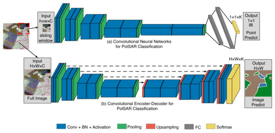
Figure 1.
Two types of deep convolutional models for PolSAR image classification. The first model (a) is a convolutional neural network with blue and green parts for feature extraction and gray and yellow parts for classification. The second model (b) is a convolutional encoder–decoder network with blue and green parts for feature extraction and red, blue, and yellow parts for classification. In both models, ‘Conv’ refers to the convolutional layer, ‘BN’ refers to the batch normalization layer, and ‘FC’ refers to the fully connected layer. The black dotted line indicates that the encoder and decoder feature maps have been fused. Additionally, ‘H’, ‘W’, and ‘C’ represent the input’s height, width, and number of channels.
Figure 1 shows that convolutional models consist of fundamental modules, including convolution, fully connected, pooling, and activation layers. Convolution and fully connected layers are linear modules while pooling, and activation layers are nonlinear modules. A complex-valued batch normalization layer [34] is commonly inserted between the convolutional and nonlinear activation layers to avoid model overfitting. Linear modules perform addition and multiplication, which can be expressed as Equations (1) and (2) for real and complex numbers.
By analyzing Equations (1) and (2), it is apparent that complex-valued addition and multiplication are linear computations of real and imaginary parts. As a result, two real-valued convolution kernels can replace one complex-valued convolution kernel, and two real-valued fully connected operators can replace one complex-valued fully connected operator.
2.2. Inputs of PolSAR Classification
The inputs with complex and real values have equal width and height but differ in the number of channels. A 2 × 2 complex-valued scattering matrix represents each resolution cell of the PolSAR data, as shown in Equation (3):
H and V represent the horizontal and vertical polarization bases in this equation, respectively. represents the backscattering coefficient between the polarization scattered and the incident field. It is typically assumed that and are identical due to the reciprocity theorem. This allows the matrix to be simplified and reduced to the scattering vector . Using the Pauli decomposition method, the scattering vector can be expressed as shown in Equation (4):
The representation of the consistency matrix for PolSAR data in the multi-look scenario can be found in Equation (5):
The equation for T, which represents the consistency matrix, includes the number of looks (L) and the conjugate transpose (denoted by H). T is a Hermitian matrix with real-valued elements on the diagonal and complex-valued elements off-diagonal. Only the upper triangular part is necessary to input T into the deep convolutional model. In the case of the real-valued model, the feature vector is represented by Equation (6) and has nine input channels:
In the model that deals with complex values, there are six input channels, and the feature vector is identified as Equation (7):
2.3. Complex-Valued Amplitude-Based Max Pooling
In machine learning, deep learning is a set of methods requiring much computational power. Unfortunately, a significant portion of this computational power is used redundantly, which can result in slow convergence, poor performance, and overfitting. One technique to address this is pooling, which reduces the amount of data involved by shrinking the feature map. Additionally, pooling also expands the receptive field, allowing the model to extract more meaningful features with contextual and global information. As a result, it is important to use pooling methods that keep the most effective features while reducing the feature map size.
Based on Figure 2a, the complex-valued feature map can be split into real and imaginary feature maps. These two maps can then be combined into an amplitude feature map. The amplitude feature map is then subjected to real-valued max pooling, and the maximum value index is recorded. Afterward, the final pooling result is obtained by utilizing the maximum index and the original feature map. The mathematical expression for amplitude-based max pooling (CVA_Max_Pooling) is shown in Equation (8):
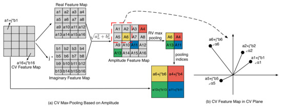
Figure 2.
(a) displays the process of amplitude-based max pooling, using gray squares to represent the feature map before pooling and colored squares for the feature map after 2 × 2 pooling. (b) shows the complex plane representation of the four features in the 2 × 2 feature map identified by the red dashed box in (a).
In this equation, F represents the feature map, while w and h refer to the width and height of the pooling kernel. Figure 2b displays a complex plane map of all the data within a pooling kernel. Each feature in this map consists of an amplitude and a phase. The amplitude indicates the strength of the feature, with higher amplitudes indicating greater strength and importance. Meanwhile, the phase of a feature indicates its synchronization relationship with other features. Features with closer phase values are more synchronized. However, comparing the two features’ phase sizes is meaningless. In Figure 2b, feature has the largest amplitude, so CVA_Max_Pooling will keep that feature in the next layer.
Complex-valued pooling methods, such as max pooling or average pooling, are commonly used on features’ real and imaginary parts. However, it is important to note that old complex-valued average pooling can weaken significant features, while old complex-valued max pooling can create “fake” features that could negatively impact the final classification results. On the other hand, CVA_Max_Pooling can efficiently preserve crucial features, thus reducing computational workload, broadening the receptive field, and enhancing classification accuracy.
2.4. Complex-Valued Nonlinear Activation
Using complex-valued nonlinear activation is beneficial in mapping features into a high-dimensional nonlinear space. This greatly enhances the nonlinear fitting ability of CV-CNNs. In RV-CNN models, the most commonly used nonlinear activations are variants of ReLU. These activations are widely used in real-valued deep learning models and deliver outstanding performance due to their computational simplicity, ease of derivation, and ability to sparsify feature maps. A simulated ReLU function is also a preferred design idea for most complex-valued nonlinear activations. Compared to real-valued activation, complex-valued activation requires a double nonlinear mapping of the feature amplitude and phase. The three common nonlinear activations in old CV-CNNs are ModReLU, CReLU, and ZReLU. Their Equations are (9)–(11), respectively.
Based on (9)–(11), it is evident that these three nonlinear activations with complex values imitate ReLU in varying ways. This paper suggests an improved complex-valued nonlinear activation called HReLU, which introduces a new approach and is expressed in Equation (12).
To fully comprehend the advantages and disadvantages of complex-valued nonlinear activations, it is crucial to understand why ReLU has succeeded in RV-CNN. ReLU is a segmented mapping with a constant mapping in the range of (−∞, 0) and a linear mapping in the range of [0, +∞). This feature makes ReLU convenient for forward inference and for the calculation of derivatives, as its derivatives are 0 in the range of (−∞, 0) and 1 in the range of . ReLU maps data in the range of to 0 while keeping data in the range of unchanged. This not only sparsifies the feature map and improves the model’s generalization ability but also prevents the feature map from being too sparse, leading to insufficient model fitting. However, for the complex-valued feature maps, the amplitude and phase ranges are and , respectively, which makes ReLU unsuitable. To address this, ModReLU, CReLU, ZreLU, and HReLU have been developed to migrate ReLU to the complex domain. If these four complex-valued nonlinear activations are split into the amplitude activation and the phase activation, they can be represented as follows:
ModReLU:
CReLU:
ZReLU:
HReLU:
By examining Figure 3 and Equations (13)–(20), it can be observed that only HReLU performs ReLU-like processing on the magnitude and phase of complex-valued feature maps. HReLU is also a segmented function, with the upper half of the complex plane being a linear mapping and the lower half being a constant mapping. Once HReLU is expressed as an amplitude-activated function and a phase-activated function, these two functions also become segmented functions, with half of the data being linear mappings and the other half being constant mappings. HReLU’s nonlinear section also maps the data as 0 + 0 · j, which sparsifies the feature map and improves the model’s generalization ability. In contrast, ModReLU’s nonlinearization range is too small, making it difficult to extract efficient features. CReLU is not sparse enough, leading to poor generalization. ZReLU is too sparse, resulting in a model prone to underfitting. According to Georgiou et al.’s complex-valued backpropagation algorithm [33], the derivatives of HReLU in the upper and lower halves of the complex plane are simple to compute, being 1 + 1 · j and 0 + 0 · j, respectively.
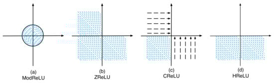
Figure 3.
(a–d) depict the complex plane mappings for ModReLU, CReLU, ZReLU, and HReLU, respectively. The blue shaded area corresponds to the data set to 0 + 0 · j, while the dashed region with arrows indicates data mapped to the coordinate axes. Any blank part areas in the data will be preserved for the next layer.
2.5. Complex-Valued Cross-Entropy
CNNs are supervised learning models that rely on the loss between the model output and the label during training. In the case of RV-CNN used for PolSAR image classification, the output is a real-valued probability distribution vector. The labels are a real-valued one-hot vector with dimensions equal to the number of categories. RV-CNN uses real-valued cross-entropy to calculate the loss of PolSAR image classification. However, CV-CNN’s output is no longer a real-valued probability distribution vector, which means that real-valued cross-entropy cannot be used to calculate the loss. The old complex-valued classification models only use the real part of the output to calculate the loss value, but this approach loses at least half of the information flow. Thus, this paper proposes a CV_one-hot label, complex-valued probability distribution vector and CV_CrossEntropy to address this issue.
2.5.1. Complex-Valued Probability and CV_one-hot Label
Complex-valued probability is an extension of traditional probability that uses complex numbers to express probability distributions [44,45,46,47,48]. Before delving into this concept, it is important to clarify some related theorems.
Definition 1.
Pm = j · (1 − Pr) represents the probability of a random event A in the imaginary and real fields, where j denotes the imaginary unit.
Theorem 1.
The norm of a random event in the complex domain is calculated as : .
Theorem 2.
The sum of probabilities of a random event’s real and imaginary parts in the complex domain is always equal to 1: .
From these theorems, it can be inferred that represents the probability of any random event happening, while represents the probability of the associated event in the imaginary domain. is a random event in the complex field given by and . The degree of knowledge and the chaos factor of a random event in the complex domain are denoted by and , respectively.
If , this means that the random event in the real domain is deterministic, and the degree of knowledge and the chaos factor of the random event in the complex domain are 1 and 0, respectively.
If , this means that the random event in the real domain is impossible, and the degree of knowledge and the chaos factor of the random event in the complex domain are 1 and 0, respectively.
When , the degree of knowledge of the random event in the complex domain is 0.5, and the chaos factor is −0.5.
This means a stochastic system in the complex domain has a constant probability equal to 1, but its degree of knowledge and chaos factor are variable. The more stable the stochastic system is, the greater its degree of knowledge, and the closer the chaos factor is to zero. This can be used to redesign the CV_one-hot label for PolSAR image classification.
In Figure 4a, the real-valued one-hot label can be seen as a probability distribution for an object belonging to a certain category with a 100% probability (the value at the activation point is 1, and the values at the other inactivation points are 0). Figure 4b proposes a K-dimensional complex-valued vector as the CV_one-hot label, with values at activation points and the values at the inactivation point. Figure 4c shows that when the complex-valued probability is decomposed into and probability, the meaning of the CV_one-hot label becomes easier to understand. At the activation point, equals 1, and equals 0, while at the inactivation point, equals 0, and equals 1. The vector represents the probability of classification and has the same meaning as the vector P, which is used to obtain the unique class of an object via softmax. If a complex-valued probability is treated as a stochastic system, the knowledge degree of any point in the CV_one-hot label equals 1, and the chaos factor equals 0. Therefore, the CV_one-hot label has the highest stability, as well as the largest knowledge degree and the smallest absolute value of the chaos factor.
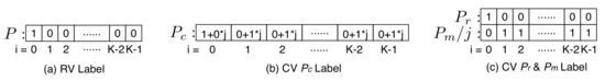
Figure 4.
(a) shows a real-valued one-hot label, while (b,c) are CV_one-hot labels. K represents the number of categories. P represents the probability of a random event in the real domain, while Pc represents the probability of a random event in the complex domain. Pr and Pm represent the real and imaginary parts of the random event in the complex domain.
2.5.2. Complex-Valued Cross-Entropy
To effectively train CV-CNNs, it is not sufficient to use CV_one-hot labels. A loss function must also measure the difference between the model’s output and the label. RV-CNNs use cross-entropy as their loss function, which calculates the difference between two probability distributions. A high loss value indicates a significant difference between the model’s output and the label, while a low value indicates a small difference. Similarly, to train CV-CNNs, this paper proposes a loss function called CV_CrossEntropy, which describes the difference between complex-valued outputs and CV_one-hot labels using the following Equation:
In Equation (23), K represents the number of categories, while N represents the number of samples in a mini-batch. In addition, y refers to the ground truth, whereas represents the model’s predicted outcome. The initial segment of the loss function only applies to the real part of the labels and the of the outputs. The smaller the value of this part, the more precise the classification outcome of the complex-valued model will be. The second part of the loss function incorporates the labels, , and of the outputs. The smaller the value of this part, the more stable the classification system will become.
2.6. Complex-Valued PolSAR Classification Algorithm
Algorithm 1 outlines the PolSAR classification process based on a complex-valued approach proposed in this research. The first step involves constructing a complex-valued convolutional classification network equipped with CVA_Max_Pooling and HReLU in the model. Next, CV_one-hot labels are applied to the training set. Then, the model parameters are updated through iterations using the CV_CrossEntropy loss. Lastly, the trained model is utilized to classify the complete PolSAR dataset.
| Algorithm 1: Complex-valued convolutional classification algorithm for PolSAR images |
| Preprocessing: 1. Construction of complex-valued models for PolSAR image classification with CVA_Max_Pooling and HReLU 2. Assigning CV_one-hot labels to each pixel of the PolSAR dataset 3. Selection of training set from the PolSAR dataset Input: a training set and corresponding labels, learning rate, batch size, and momentum parameter 4. Repeat: 5. Calling CVA_Max_Pooling to obtain the most efficient features 6. Invoking HReLU to map the amplitude and phase of the feature to the nonlinear domain 7. Calling CV_CrossEntropy to compute the loss during training 8. Updating model parameters with loss 9. Until: Meeting the conditions for termination 10. Inferring the class of the entire PolSAR image with the trained model Output: Prediction of the testing set |
3. Experimental Results
This section will start by providing a brief description of the three benchmark datasets. Subsequently, the section delves into the specifics of the model inputs, the experimental setup, and the evaluation metrics. Finally, the effectiveness of the proposed complex-valued approach is demonstrated through a comparative analysis of classification model results across the three PolSAR datasets.
3.1. PolSAR Dataset Description
3.1.1. Flevoland Dataset 1
On 16 August 1989, the NASA/JPL AIRSAR airborne platform collected a dataset from the Flevoland area in the Netherlands. These data have a size of 750 × 1024, and Figure 5a,b displays the RGB image and corresponding ground truth after Pauli decomposition. The image contains 15 categories: stembeans, peas, forest, lucerne, wheat, beet, potatoes, bare soil, grass, rapeseed, barley, wheat2, wheat3, water, and buildings.
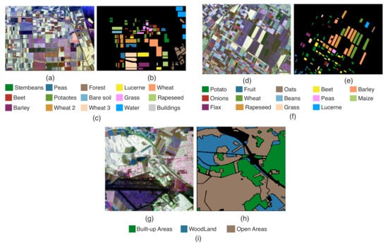
Figure 5.
The ground truth and class legends of Flevoland Dataset 1, Flevoland Dataset 2, and Oberpfaffenhofen Dataset. (a,d,g) are RGB images, (b,e,h) are the corresponding ground truth images after Pauli decomposition, and (c,f,i) are class legends.
3.1.2. Flevoland Dataset 2
In 1991, L-band ATRSAR data were collected in the Flevoland area, consisting of a size of 1024 × 1024. Figure 5d displays the RGB image, while Figure 5e shows the ground truth after Pauli decomposition. The image consists of 14 categories: potato, fruit, oats, beet, barley, onions, wheat, beans, peas, maize, flax, rapeseed, grass, and lucerne.
3.1.3. Oberpfaffenhofen Dataset
The German Aerospace Center (DLR) has provided the ESAR data for the Oberpfaffenhofen area in Germany. The dataset is 1300 × 1200, and the RGB image and the corresponding ground truth after Pauli decomposition are displayed in Figure 5g,h. The image depicts three categories: built-up, woodland, and open areas.
3.2. Parameterization
Before conducting experiments, it is crucial to establish the appropriate training. For PolSAR image classification, several studies have explored the sampling rate and neural network parameters for PolSAR image classification [20], which renders it unnecessary for this paper to delve into those parameters. Instead, this paper will utilize them directly in the experiments.
Training and testing sets for SCNN, DCNN, FCN, and SegNet needed to be created using PolSAR images and labels. The inputs and outputs for these models were explained in Section 2.1 and will not be repeated here. For the SCNN and DCNN, the input was a 12 × 12 image patch containing a pixel to be classified. For FCN and SegNet, a sliding window of 128 × 128 with a sliding step of 15 generated training and testing sets on PolSAR images and labels. Only labeled pixels in the input of FCN and SegNet were involved in training, and unlabeled pixels could not be used to update model parameters. In all experiments, the model was trained and validated using a ratio of 0.9/0.1 for pixels in the training set.
PyTorch was employed for implementing all codes, and the Adam optimizer with default parameters was utilized. All experiments were conducted on a single workstation with an Intel Core i7-6700K CPU, 32G RAM, an NVIDIA TITAN X GPU, and an Ubuntu 20.04 LTS operating system.
3.3. Evaluation Metrics
When evaluating how well PolSAR images are classified, there are three common metrics: overall accuracy (OA), average accuracy (AA), and Kappa coefficient. OA is the ratio of correctly classified samples to the number of test samples. AA is the average accuracy of classification for each category. The kappa coefficient is a metric that measures the effectiveness of classification and consistency testing, especially when the number of samples in different categories varies greatly. The larger these metrics, the better the classification effect.
3.4. Model Parameters
The SCNN, DCNN, FCN, and SegNet parameters are listed in Table 1, Table 2 and Table 3, respectively. For real-valued models, ReLU was used as the activation function, max pooling was used as the pooling function, and cross-entropy was used as the loss function. For old complex-valued models, CReLU was used as the activation function, max pooling was used as the pooling function, and cross-entropy was used as the loss function. For new complex-valued models, HReLU was used as the activation function, CVA_Max_Pooling was used as the pooling function, and CV_CrossEntropy was used as the loss function. To ensure fairness in the experiment, the number of parameters in the different models was kept as equal as possible.

Table 1.
Detailed parameters of the RV-SCNN and CV-SCNN. K denotes the total number of categories.
Table 2.
Detailed parameters of the RV-DCNN and CV-DCNN. K denotes the total number of categories.
Table 3.
Detailed parameters of the RV-(FCN, SegNet) and CV-(FCN, SegNet). K denotes the total number of categories.
3.5. Analysis of Experimental Results
3.5.1. Flevoland Dataset 1 Results
In order to enhance the robustness assessment of the proposed methods, cross-validation was employed to acquire the classification results. Five percent of the labeled samples from each of the 15 dataset categories were randomly selected as the training set, while the remaining samples constituted the testing set. The final result, as depicted in Figure 6 and Table 4, represents the average of ten classification outcomes.
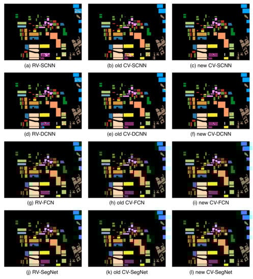
Figure 6.
Classification results of Flevoland Dataset 1 with different methods. The classification results of RV-SCNN, RV-DCNN, RV-FCN, and RV-SegNet are represented by (a,d,g,j), respectively, while the results of old CV-SCNN, old CV-DCNN, old CV-FCN, and old CV-SegNet are shown by (b,e,h,k). The classification results of new CV-SCNN, new CV-DCNN, new CV-FCN, and new CV-SegNet are represented by (c,f,i,l).
Table 4.
Overall accuracy (%), average accuracy (%), and Kappa coefficient of all competing methods on the Flevoland Dataset 1. The bolded values represent the highest values among three versions of a model (RV-, old CV-, new CV-).
It is evident from the quantitative results that the real-valued version of any classification model has the poorest classification results, while the new complex-valued approach has the best results. This demonstrates the effectiveness of the new complex-valued approach. The complex-valued approach preserves the phase features of the input, thus extracting and retaining more effective features. Moreover, CVA_Max_Pooling preserves the most discriminative features, while HReLU provides sufficient nonlinearity and sparsity. Finally, CV_CrossEntropy enhances the efficiency of feature utilization, leading to the best classification results.
After analyzing the effects of four classification models, it was observed that SegNet performs the best in achieving classification results under the same version, while SCNN has the poorest classification results, and the encoder–decoder model outperforms the CNN model. The new CV-SCNN, new CV-DCNN, new CV-FCN, and new CV-SegNet have shown an improvement of 4.01%, 4.46%, 3.46%, and 0.45%, respectively, over RV-SCNN, RV-DCNN, RV-FCN, and RV-SegNet. The results indicate that the complex-valued method has a significant improvement effect on CNNs with fewer parameters. This is because the classification results of FCN and SegNet are already satisfactory, and improving them significantly using the complex-valued method is challenging. Therefore, if only CNNs can be selected for PolSAR image classification due to machine performance constraints, the new CV-CNN model would be the best choice. Otherwise, the new CV-SegNet would provide optimal classification results. Figure 6l highlights that the new CV-SegNet’s results are almost identical to the ground truth.
3.5.2. Flevoland Dataset 2 Results
In order to enhance the robustness assessment of the proposed methods, cross-validation was employed to acquire the classification results. Five percent of the labeled samples from each of the 14 dataset categories were randomly selected as the training set, while the remaining samples constituted the testing set. The final result, as depicted in Figure 7 and Table 5, represents the average of ten classification outcomes.
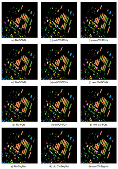
Figure 7.
Classification results of Flevoland Dataset 2 with different methods. The classification results of RV-SCNN, RV-DCNN, RV-FCN, and RV-SegNet are represented by (a,d,g,j), respectively, while the results of old CV-SCNN, old CV-DCNN, old CV-FCN, and old CV-SegNet are shown by (b,e,h,k). The classification results of new CV-SCNN, new CV-DCNN, new CV-FCN, and new CV-SegNet are represented by (c,f,i,l).
Table 5.
Overall accuracy (%), average accuracy (%), and Kappa coefficient of all competing methods on the Flevoland Dataset 2. The bolded values represent the highest values among three versions of a model (RV-, old CV-, new CV-).
According to Table 5, FCN and SegNet can extract more contextual information, resulting in excellent classification results for (RV-, old CV-, new CV-) FCN and SegNet. Although the new CV-FCN and new CV-SegNet perform the best in classification, the improvement is not very noticeable. In comparison, new CV-SCNN and new CV-DCNN show a significant improvement in their classification results compared to RV-SCNN and RV-DCNN. It is worth noting that RV-SCNN and RV-DCNN only achieve 0.09% and 11.18% accuracy, respectively, for the category of beans, while old CV-SCNN and old CV-DCNN only achieve 13.29% and 17.89% accuracy for the onions category. In contrast, the new CV-SCNN and new CV-DCNN show a more balanced performance in these two categories, with no extremely low accuracy. The new CV-SCNN has a classification accuracy of 82.16% and 60% for beans and onions, respectively, while the new CV-DCNN has a classification accuracy of 98.63% and 76.24% for beans and onions, respectively.
From Figure 5e, it is apparent that both beans and onions fall under categories with a limited number of samples. The RV-CNNs and old CV-CNNs have struggled to extract the features of these categories during training. This is because the inputs of these categories have only a few complex-valued features hidden in them. RV-CNNs ignore this part of the features from the input, while old CV-CNNs destroy it during the computation process. However, the new CV-CNNs are designed to retain this part of the features as much as possible during computation. Hence, they can accurately recognize beans and onions.
3.5.3. Oberpfaffenhofen Dataset Results
In order to enhance the robustness assessment of the proposed methods, cross-validation was employed to acquire the classification results. Only one percent of the labeled samples from each of the three dataset categories were randomly selected as the training set, while the remaining samples constituted the testing set. The final result, as depicted in Figure 8 and Table 6, represents the average of ten classification outcomes.
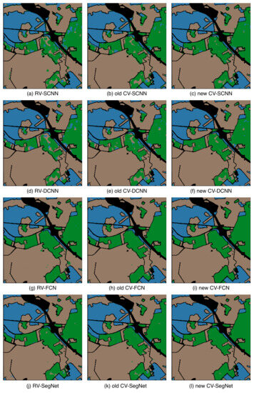
Figure 8.
Classification results of Oberpfaffenhofen Dataset with different methods. The classification results of RV-SCNN, RV-DCNN, RV-FCN, and RV-SegNet are represented by (a,d,g,j), respectively, while the results of old CV-SCNN, old CV-DCNN, old CV-FCN, and old CV-SegNet are shown by (b,e,h,k). The classification results of new CV-SCNN, new CV-DCNN, new CV-FCN, and new CV-SegNet are represented by (c,f,i,l).
Table 6.
Overall accuracy (%), average accuracy (%), and Kappa coefficient of all competing methods on the Oberpfaffenhofen Dataset. The bolded values represent the highest values among three versions of a model (RV-, old CV-, new CV-).
Table 6 shows that all models can accurately classify woodland and open areas with classification accuracies above 96%. However, Figure 8a–f shows that CNNs sometimes confuse built-up areas with woodland. Nonetheless, according to Table 6, the classification accuracy of the new CV-SCNN for built-up areas is higher than that of RV-SCNN and old CV-SCNN by 12.6% and 5.14%, respectively. Additionally, the new CV-DCNN has a classification accuracy for built-up areas that is 10.45% and 7% higher than that of RV-DCNN and old CV-DCNN, respectively. These results suggest that the new complex-valued approach significantly improves the classification accuracy of the more challenging categories.
In summary, it is recommended to use SegNet instead of CNNs to enhance the accuracy of PolSAR image classification without any restrictions on the model size. Although the new CV-SegNet offers better classification outcomes than RV-SegNet, the accuracy improvement is limited. When the model size is limited, the optimal choice is the new CV-CNNs, which can accurately distinguish difficult entries and significantly improve the classification accuracy of small sample categories, thus leading to an overall enhancement in accuracy.
3.5.4. Computational Complexity of CNN
From Figure 9a,b, Table 1 and Table 2, it is evident that when the number of convolutional layers in CV-CNN and RV-CNN is the same and the difference in the number of parameters is not substantial, CV-CNN has fewer convolutional kernels in each layer, yet achieves higher classification accuracy. This indicates that, despite extracting fewer feature maps, the new CV-CNN consistently delivers superior classification results.
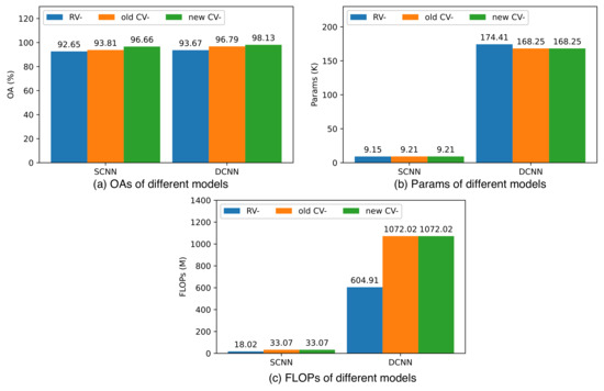
Figure 9.
(a–c) illustrate the overall accuracy, number of parameters, and FLOPs (floating-point operations per second) for SCNN and DCNN on the Flevoland Dataset 1, respectively. The blue color represents the real-valued version, the red color corresponds to the old complex-valued version, and the green color indicates the new complex-valued version.
Figure 9b,c illustrates that the FLOPs of CV-CNN are significantly larger than those of RV-CNN when they share the same number of convolutional layers and the difference in the number of parameters is not substantial. This discrepancy arises because complex-valued operations can only be approximated by multiple real-valued operations in the PyTorch environment, as depicted in Formulas (1) and (2). For instance, a complex-valued addition operation necessitates two real-valued addition operations, while a complex multiplication operation requires four real-valued multiplication operations and two real-valued addition operations. It is expected that with advancements in complex-valued deep learning techniques, particularly in polarized coordinates, where a real-valued multiplication operation and a real-valued addition operation can replace a complex-valued multiplication operation, this limitation will be mitigated.
Comparing the old CV-CNN and new CV-CNN with the same number of parameters and FLOPs, the new CV-CNN consistently outperforms the old CV-CNN, achieving better classification results. For the Flevoland Dataset 1, the new CV-SCNN yields a 2.99% higher accuracy than RV-DCNN and is only 0.1% lower than the old CV-DCNN. For the Flevoland Dataset 2, the new CV-SCNN achieves results 2% higher than RV-DCNN and 1% higher than the old CV-DCNN. In essence, under the condition of meeting accuracy requirements, the new CV-SCNN can effectively replace RV-DCNN and the old CV-DCNN. Moreover, the new CV-SCNN boasts approximately half the parameters compared to RV-DCNN and old CV-DCNN, with FLOPs being roughly half of RV-DCNN and about one-third of old CV-DCNN. This trend holds for the Oberpfaffenhofen Dataset as well.
4. Discussion
Three ablation experiments were conducted to validate the performance of various aspects of the new CV-DL models, specifically CVA_Max_Pooling, HReLU, and CV_CrossEntropy. The SCNN classification model was chosen and validated on three different datasets.
4.1. Ablation Experiment 1: Performance of CVA_Max_Pooling
One of the new components in CV-DL models is CVA_Max_Pooling. This component is important because it helps to retain the most important features in the feature map and passes them on to the next convolution layer. This increases the feature utilization efficiency and reduces the computation required. To test the impact of CVA_Max_Pooling on the experimental results, complex-valued classification models were created using both real-valued max pooling and average pooling. These models operate on the real and imaginary parts of the feature map separately. Table 7 shows the results of our experiments, with RMP-CV-SCNN and RAP-CV-SCNN denoting the models using real-valued max pooling and average pooling, respectively.
Table 7.
Overall accuracy (%), average accuracy (%), and Kappa coefficient of the different poolings.
Table 7 shows that the new CV-SCNN achieved the best classification results on all three datasets, followed by RMP-CV-SCNN, while RAP-CV-SCNN obtained the worst outcome. Notably, CVA_Max_Pooling is superior to max pooling, as it not only retains the most significant features but also avoids generating “fake” features. Max pooling tends to generate “fake” features by operating on the real and imaginary parts of the feature map separately, resulting in two unrelated features being combined. Although average pooling works on the real and imaginary parts separately, it is a form of complex-valued average pooling. While it does not generate “fake” features, it significantly reduces the weight of the most important features by confusing them with the unimportant ones.
4.2. Ablation Experiment 2: Performance of HReLU
HReLU functions as a complex-domain ReLU by discarding half of the features nonlinearly. To assess its effects on experimental results, complex-valued classification models were created using ModReLU, ZreLU, and CReLU, referred to as Mod-CV-SCNN, ZReLU-CV-SCNN, and CReLU-CV-SCNN, respectively. The outcomes of these experi-ments can be found in Table 8.
Table 8.
Overall accuracy (%), average accuracy (%), and Kappa coefficient of the different activations.
Based on the data presented in Table 8, it is clear that new CV-SCNN outperforms the other models on all three datasets. Additionally, CReLU-CV-SCNN yields better results than ZReLU-CV-SCNN and Mod-CV-SCNN, despite both containing ReLU in their names. However, as explained in Section 2.3, only HReLU produces ReLU-like sparsity and nonlinearity. CReLU is slightly less effective due to a lack of sparsity, while ZReLU underperforms because too many features are dropped, and ModReLU produces the worst results due to its inadequate nonlinearity.
4.3. Ablation Experiment 3: Performance of CV_CrossEntropy
When training deep learning models, the loss function is crucial in driving the model outputs closer to the ground truth and helping the model learn the best classification patterns. For complex domain classification tasks, the CV_CrossEntropy loss function is commonly used in conjunction with complex-valued probabilities to continuously improve the model’s accuracy and stability during training. Two common methods for combining cross-entropy and CV-CNN are: (i) calculating cross-entropy loss using only the output’s real part and (ii) calculating cross-entropy loss using the real and imaginary parts of the output separately and then summing them up as the final loss. However, the second approach contains a logical error that arises when the model outputs different classification results using real and imaginary parts, leading to confusion.
To assess the influence of CV_CrossEntropy on the experimental outcomes, a complex-valued classification model was developed to utilize real-valued cross-entropy ((i) calculating cross-entropy loss using only the output’s real part), called RCE-CV-SCNN. The findings of the experiment are presented in Table 9.
Table 9.
Overall accuracy (%), average accuracy (%), and Kappa coefficient of the different loss functions.
According to Table 9, CV-SCNN performs better than RCE-CV-SCNN in all three experiments. This is because CV-SCNN produces complex-valued output, while RCE-CV-SCNN can only calculate the loss using the real part of the output. This results in the loss of half of the information flow. Additionally, the constraints imposed on the model by CV_CrossEntropy are stronger than RV_CrossEntropy, which helps the model learn more accurate classification patterns.
Figure 10 illustrates the training progression of the new CV-SCNN and RCE-CV-SCNN models on Flevoland Dataset 1. Despite the heightened computational complexity and the imposition of more stringent constraints associated with the computation of CV_CrossEntropy, the convergence rate of the models remains unimpeded. Over successive epochs, the new CV-SCNN exhibits a gradual improvement in accuracy over RCE-CV-SCNN. It is pertinent to note that even though the new CV-SCNN consistently manifests higher loss values compared to RCE-CV-SCNN during the convergence phase, this discrepancy arises from the augmented computational elements within CV_CrossEntropy and does not detrimentally impact the overall model performance.
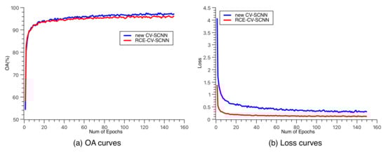
Figure 10.
(a,b) each represent the variation curves of overall accuracy and loss function during the training process for RCE-CV-SCNN and new CV-SCNN.
4.4. Comparison with State-of-the-Art Algorithms
This study also conducted a comparison on Flevoland Dataset 1, evaluating the new CV-SegNet against the state-of-the-art algorithms, with results presented in Table 10. The findings reveal that the new CV-SegNet achieves the highest classification performance. However, it is worth noting that such comparisons may lack full rigor due to the diverse research objectives associated with each algorithm. Consequently, they employ inputs of varying sizes and training datasets with different sampling rates, all of which can influence the final outcomes. For example, RCV-CNN excels in achieving superior accuracy when confronted with limited annotated data, a proficiency that may not confer significant advantages when dealing with relatively large training datasets. The method proposed in this paper is not an independent model but rather an approach aimed at enhancing deep learning models, including CNNs, FCNs, and SegNets. The resulting improved models can lead to performance enhancements or reductions in parameter complexity.
Table 10.
Overall accuracy (%), average accuracy (%), and Kappa coefficient of the state-of-the-art algorithms on the Flevoland Dataset 1. The bolded values represent the highest values among all models.
5. Conclusions
This paper introduced a new method for enhancing deep learning models utilized in PolSAR image classification. The method involves CVA_Max_Pooling, HReLU, and CV_CrossEntropy. CVA_Max_Pooling decreases the computational work and extracts the most important features. HReLU changes the model into a nonlinear sparse model, while CV_CrossEntropy provides a loss computation method for complex-domain classification tasks. The proposed complex-valued deep learning method was applied to improve four PolSAR classification models: SCNN, DCNN, FCN, and SegNet. The models were then validated on three public PolSAR datasets. The experimental results reveal that the method proposed in this paper outperforms the old complex-valued model and is much better than the real-valued model despite having comparable parameters.
In order to continue this work in the future, the following ideas could be explored: (1) While the experiments have shown that the new complex-valued method can significantly improve the performance of shallow CNNs, it is important to note that the inference process of CNNs can be quite time-consuming. On the other hand, FCNs are effective at fast inference but require many model parameters and computation. Therefore, it would be worthwhile to explore the possibility of combining the new complex-valued method with shallow FCNs to improve classification accuracy and reduce inference time simultaneously; (2) The experiments have also demonstrated that the new complex-valued method is suitable for learning with small samples. Further research could be conducted to reduce the sampling rate by utilizing the new complex-valued method.
Author Contributions
Conceptualization, Y.R.; data curation, Y.R.; methodology, Y.R.; supervision, Y.L.; validation, W.J.; writing–original draft, Y.R.; writing–review and editing, W.J. and Y.L. All authors have read and agreed to the published version of the manuscript.
Funding
This work was supported in part by the National Natural Science Foundation of China under Grant #62176247 and research grant #2020-JCJQ-ZD-057-00. It was also supported by the Fundamental Research Funds for the Central Universities.
Data Availability Statement
The datasets utilized in the experiments are accessible to the public and can be accessed from the following website: https://earth.esa.int/eogateway/campaigns/agrisar (accessed on 16 August 2022).
Acknowledgments
The authors wish to extend our thanks to Cheng Wang and the other researchers in Beijing Raying Technologies, Inc. for their great support in radar data analysis.
Conflicts of Interest
The authors declare no conflict of interest.
References
- Lee, J.S.; Pottier, E. Polarimetric Radar Imaging: From Basic to Application; CRC Press: Boca Raton, FL, USA, 2011; pp. 1–22. [Google Scholar]
- Hänsch, R.; Hellwich, O. Skipping the real world: Classification of PolSAR images without explicit feature extraction. ISPRS J. Photogramm. Remote Sens. 2018, 140, 122–132. [Google Scholar] [CrossRef]
- Lee, J.S.; Grunes, M.R.; Kwok, R. Classification of multi-look polarimetric SAR imagery based on the complex Wishart distribution. Int. J. Remote Sens. 1994, 15, 2299–2311. [Google Scholar] [CrossRef]
- Lee, J.S.; Grunes, M.R.; Pottier, E.; Ferro-Famil, L. Unsupervised terrain classification preserving polarimetric scattering characteristics. IEEE Trans. Geosci. Remote Sens. 2004, 42, 722–731. [Google Scholar] [CrossRef]
- Dabboor, M.; Collins, M.; Karathanassi, V.; Braun, A. An unsupervised classification approach for polarimetric SAR data based on the Chernoff distance for the complex Wishart distribution. IEEE Trans. Geosci. Remote Sens. 2013, 51, 4200–4213. [Google Scholar] [CrossRef]
- Wu, Y.; Ji, K.; Yu, W.; Su, Y. Region-based classification of polarimetric SAR images using Wishart MRF. IEEE Geosci. Remote Sens. Lett. 2008, 5, 668–672. [Google Scholar] [CrossRef]
- Song, W.; Li, M.; Zhang, P.; Wu, Y.; Tan, X.; An, L. Mixture WGΓ-MRF model for PolSAR image classification. IEEE Trans. Geosci. Remote Sens. 2018, 56, 905–920. [Google Scholar] [CrossRef]
- Arii, M.; van Zyl, J.J.; Kim, Y. Adaptive model-based decomposition of polarimetric SAR covariance matrices. IEEE Trans. Geosci. Remote Sens. 2011, 49, 1104–1113. [Google Scholar] [CrossRef]
- Clound, S.R.; Pottier, E. An entropy based classification scheme for land applications of polarimetric SAR. IEEE Trans. Geosci. Remote Sens. 1997, 35, 68–78. [Google Scholar] [CrossRef]
- Cloude, S.R.; Pottier, E. A review of target decomposition theorems in radar polarimetry. IEEE Trans. Geosci. Remote Sens. 1996, 34, 498–518. [Google Scholar] [CrossRef]
- An, W.; Cui, Y.; Yang, J. Three-Component Model-Based Decomposition for Polarimetric SAR Data. IEEE Trans. Geosci. Remote Sens. 2010, 48, 2732–2739. [Google Scholar] [CrossRef]
- He, C.; Li, S.; Liao, Z.; Liao, M. Texture Classification of PolSAR Data Based on Sparse Coding of Wavelet Polarization Textons. IEEE Trans. Geosci. Remote Sens. 2013, 51, 4576–4590. [Google Scholar] [CrossRef]
- Lardeux, C.; Frison, P.L.; Tison, C.C.; Souyris, J.C.; Stoll, B.; Fruneau, B.; Rudant, J.P. Support vector machine for multifrequency SAR polarimetric data classification. IEEE Trans. Geosci. Remote Sens. 2009, 47, 4143–4152. [Google Scholar] [CrossRef]
- Melgani, F.; Hashemy, B.A.R.A.; Taha, S.M.R. An explicit fuzzy supervised classification method for multispectral remote sensing images. IEEE Trans. Geosci. Remote Sens. 2000, 38, 287–295. [Google Scholar] [CrossRef]
- Ulaby, F.T.; Elachi, C. Radar polaritnetry for geoscience applications. Geocarto Int. 1990, 5, 38. [Google Scholar] [CrossRef]
- Freeman, A.; Durden, S.L. A three-component scattering model for polarimetric SAR data. IEEE Trans. Geosci. Remote Sens. 1998, 36, 963–973. [Google Scholar] [CrossRef]
- Huynen, J.R. Phenomenological Theory of Radar Targets. Available online: http://resolver.tudelft.nl/uuid:e4a140a0-c175-45a7-ad41-29b28361b426 (accessed on 14 April 2022).
- De, S.; Bruzzone, L.; Bhattacharya, A.; Bovolo, F.; Chaudhuri, S. A Novel Technique Based on Deep Learning and a Synthetic Target Database for Classification of Urban Areas in PolSAR Data. IEEE J. Sel. Top. Appl. Earth Obs. Remote Sens. 2018, 11, 154–170. [Google Scholar] [CrossRef]
- Zhou, Y.; Wang, H.; Xu, F.; Jin, Y.Q. Polarimetric SAR image classification using deep convolutional neural networks. IEEE Geosci. Remote Sens. Lett. 2016, 13, 1935–1939. [Google Scholar] [CrossRef]
- Bin, H.; Sun, J.; Xu, Z. A Graph-Based Semisupervised Deep Learning Model for PolSAR Image Classification. IEEE Trans. Geosci. Remote Sens. 2019, 57, 2116–2132. [Google Scholar] [CrossRef]
- Li, Y.; Chen, Y.; Liu, G.; Jiao, L. A novel deep fully convolutional network for PolSAR image classification. Remote Sens. 2018, 10, 1984. [Google Scholar] [CrossRef]
- Pham, M.; Lefevre, S. Very high resolution Airborne PolSAR Image Classification using Convolutional Neural Networks. In Proceedings of the 13th European Conference on Synthetic Aperture Radar (EUSAR 2021), Online, 29 March–1 April 2021; pp. 1–4. [Google Scholar]
- Liu, S.; Luo, H.; Shi, Q. Active Ensemble Deep Learning for Polarimetric Synthetic Aperture Radar Image Classification. IEEE Geosci. Remote Sens. Lett. 2021, 18, 1580–1584. [Google Scholar] [CrossRef]
- Cheng, J.; Zhang, F.; Xiang, D.; Yin, Q.; Zhou, Y. PolSAR Image Classification with Multiscale Superpixel-Based Graph Convolutional Network. IEEE Trans. Geosci. Remote Sens. 2022, 60, 1–14. [Google Scholar] [CrossRef]
- Liu, G.; Li, Y.; Jiao, L.; Chen, Y.; Shang, R. Multiobjective evolutionary algorithm assisted stacked autoencoder for PolSAR image classification. Swarm Evol. Comput. 2021, 60, 100794. [Google Scholar] [CrossRef]
- Jing, H.; Wang, Z.; Sun, X.; Xiao, D.; Fu, K. PSRN: Polarimetric Space Reconstruction Network for PolSAR Image Semantic Segmentation. IEEE J. Sel. Top. Appl. Earth Obs. Remote Sens. 2021, 14, 10716–10732. [Google Scholar] [CrossRef]
- Nie, W.; Huang, K.; Yang, J.; Li, P. A Deep Reinforcement Learning-Based Framework for PolSAR Imagery Classification. IEEE Trans. Geosci. Remote Sens. 2022, 60, 1–15. [Google Scholar] [CrossRef]
- Yang, C.; Hou, B.; Chanussot, J.; Hu, Y.; Ren, B.; Wang, S.; Jiao, L. N-Cluster Loss and Hard Sample Generative Deep Metric Learning for PolSAR Image Classification. IEEE Trans. Geosci. Remote Sens. 2022, 60, 1–16. [Google Scholar] [CrossRef]
- Ren, B.; Zhao, Y.; Hou, B.; Chanussot, J.; Jiao, L. A Mutual Information-Based Self-Supervised Learning Model for PolSAR Land Cover Classification. IEEE Trans. Geosci. Remote Sens. 2021, 59, 9224–9237. [Google Scholar] [CrossRef]
- Lee, J.S.; Hoppel, K.W.; Mango, S.A.; Miller, A.R. Intensity and phase statistics of multilook polarimetric and interferometric SAR imagery. IEEE Trans. Geosci. Remote Sens. 1994, 32, 1017–1028. [Google Scholar] [CrossRef]
- Ainsworth, T.L.; Kelly, J.P.; Lee, J.S. Classification comparisons between dual-pol, compact polarimetric and quad-pol SAR imagery. ISPRS J. Photogramm. Remote Sens. 2009, 64, 464–471. [Google Scholar] [CrossRef]
- Turkar, V.; Deo, R.; Rao, Y.S.; Mohan, S.; Das, A. Classification accuracy of multi-frequency and multi-polarization SAR images for various land covers. IEEE J. Sel. Top. Appl. Earth Obs. Remote Sens. 2012, 5, 936–941. [Google Scholar] [CrossRef]
- Georgiou, G.M.; Koutsougeras, C. Complex domain backpropagation. IEEE Trans. Circuits Syst. II Analog Digital Signal Process. 1992, 39, 330–334. [Google Scholar] [CrossRef]
- Trabelsi, C.; Bilaniuk, O.; Zhang, Y.; Serdyuk, D.; Subramanian, S.; Santos, J.; Mehri, S.; Rostamzadeh, N.; Bengio, Y.; Pal, C. Deep complex networks. In Proceedings of the International Conference on Learning Representations (ICLR2018), Vancouver, BC, Canada, 30 April–3 May 2018. [Google Scholar]
- Zhang, Z.; Wang, H.; Xu, F.; Jin, Y. Complex-Valued Convolutional Neural Network and Its Application in Polarimetric SAR Image Classification. IEEE Trans. Geosci. Remote Sens. 2017, 55, 7177–7188. [Google Scholar] [CrossRef]
- Li, L.; Ma, L.; Jiao, L.; Liu, F.; Sun, Q.; Zhao, J. Complex Contourlet-CNN for polarimetric SAR image classification. Pattern Recognit. 2020, 100, 107110. [Google Scholar] [CrossRef]
- Xiao, D.; Liu, C.; Wang, Q.; Wang, C.; Zhang, X. PolSAR Image Classification Based on Dilated Convolution and Pixel-Refining Parallel Mapping network in the Complex Domain. arXiv 2020, arXiv:1909.10783. [Google Scholar]
- Zhao, J.; Datcu, M.; Zhang, Z.; Xiong, H.; Yu, W. Contrastive-Regulated CNN in the Complex Domain: A Method to Learn Physical Scattering Signatures From Flexible PolSAR Images. IEEE Trans. Geosci. Remote Sens. 2019, 57, 10116–10135. [Google Scholar] [CrossRef]
- Tan, X.; Li, M.; Zhang, P.; Wu, Y.; Song, W. Complex-Valued 3-D Convolutional Neural Network for PolSAR Image Classification. IEEE Geosci. Remote Sens. Lett. 2020, 17, 1022–1026. [Google Scholar] [CrossRef]
- Zhang, P.; Tan, X.; Li, B.; Jiang, Y.; Song, W.; Li, M.; Wu, Y. PolSAR Image Classification Using Hybrid Conditional Random Fields Model Based on Complex-Valued 3-D CNN. IEEE Trans. Aerosp. Electron. Syst. 2021, 57, 1713–1730. [Google Scholar] [CrossRef]
- Qin, X.; Hu, T.; Zou, H.; Yu, W.; Wang, P. Polsar Image Classification via Complex-Valued Convolutional Neural Network Combining Measured Data and Artificial Features. In Proceedings of the 2019 IEEE International Geoscience and Remote Sensing Symposium (IGARSS2019), Yokohama, Japan, 28 July–2 August 2019; pp. 3209–3212. [Google Scholar]
- Fang, Z.; Zhang, G.; Dai, Q.; Xue, B. PolSAR Image Classification Based on Complex-Valued Convolutional Long Short-Term Memory Network. IEEE Geosci. Remote Sens. Lett. 2022, 19, 1–5. [Google Scholar] [CrossRef]
- Tan, X.; Li, M.; Zhang, P.; Wu, Y.; Song, W. Deep Triplet Complex-Valued Network for PolSAR Image Classification. IEEE Trans. Geosci. Remote Sens. 2021, 59, 10179–10196. [Google Scholar] [CrossRef]
- Abdo, A.J. The paradigm of complex probability and the Brownian motion. Syst. Sci. Control Eng. 2015, 3, 478–503. [Google Scholar] [CrossRef]
- Abdo, A.J. The paradigm of complex probability and Chebyshev’s inequality. Syst. Sci. Control Eng. 2016, 4, 99–137. [Google Scholar] [CrossRef]
- Abdo, A.J. The paradigm of complex probability and Claude Shannon’s information theory. Syst. Sci. Control Eng. 2017, 5, 380–425. [Google Scholar] [CrossRef]
- Abdo, A.J. The paradigm of complex probability and Ludwig Boltzmann’s entropy. Syst. Sci. Control Eng. 2018, 6, 108–149. [Google Scholar] [CrossRef]
- Abdo, A.J. The paradigm of complex probability and Monte Carlo methods. Syst. Sci. Control Eng. 2019, 7, 407–451. [Google Scholar] [CrossRef]
- Xie, W.; Ma, G.; Zhao, F.; Liu, H.; Zhang, L. PolSAR image classification via a novel semi-supervised recurrent complex-valued convolution neural network. Neurocomputing 2020, 388, 255–268. [Google Scholar] [CrossRef]
- Shang, R.; Wang, J.; Jiao, L.; Yang, X.; Li, Y. Spatial feature-based convolutional neural network for PolSAR image classification. Appl. Soft Comput. 2022, 123, 108922. [Google Scholar] [CrossRef]
- Hua, W.; Wang, X.; Zhang, C.; Jin, X. Attention-Based Multiscale Sequential Network for PolSAR Image Classification. IEEE Geosci. Remote Sens. Lett. 2022, 19, 1–5. [Google Scholar] [CrossRef]
Disclaimer/Publisher’s Note: The statements, opinions and data contained in all publications are solely those of the individual author(s) and contributor(s) and not of MDPI and/or the editor(s). MDPI and/or the editor(s) disclaim responsibility for any injury to people or property resulting from any ideas, methods, instructions or products referred to in the content. |
© 2023 by the authors. Licensee MDPI, Basel, Switzerland. This article is an open access article distributed under the terms and conditions of the Creative Commons Attribution (CC BY) license (https://creativecommons.org/licenses/by/4.0/).