Abstract
The deep learning technique has already been successfully applied in the field of microwave remote sensing. Especially, convolutional neural networks have demonstrated remarkable effectiveness in synthetic aperture radar (SAR) image semantic segmentation. In this paper, a Lovász-softmax loss optimization SAR net (LoSARNet) is proposed which optimizes the semantic segmentation metric intersection over union (IOU) instead of using the traditional cross-entropy loss. Meanwhile, making use of the advantages of the dual-path structure, the network extracts feature through the spatial path (SP) and the context path (CP) to achieve a balance between efficiency and accuracy. Aiming at a polarimetric SAR (PolSAR) image, the proposed network is conducted on the PolSAR datasets for terrain segmentation. Compared to the typical dual-path network, which is the bilateral segmentation network (BiSeNet), the proposed LoSARNet can obtain better mean intersection over union (MIOU). And the proposed network also shows the highest evaluation index and the best performance when compared with several typical networks.
1. Introduction
Synthetic aperture radar (SAR) is a crucial remote sensing technique for realizing high-resolution earth observation under all weather conditions and all time conditions. As an active imaging radar, SAR demonstrates significant capabilities in both civil and military fields, playing a vital role in remote sensing applications [1,2,3]. Through SAR image interpretation, a large scene investigation can be achieved [4,5]. Unlike optical images, SAR images are hard to use effectively by only visual interpretation; the interpretation of polarimetric SAR images especially is more difficult [6,7]. With the increasing availability of high-resolution SAR, including PolSAR, image products from airborne and spaceborne systems, the segmentation of land cover is still a hot topic in SAR applications. However, the massive amount of SAR data brings broad prospects and formidable challenges.
Still considered the foundation for wide terrain investigation, SAR image classification is frequently used in urban segmentation, road extraction, crop classification, change detection, and other applications [8,9,10,11]. The traditional classification methods are mainly based on statistical distribution and a physical scattering mechanism, such as the wavelet feature and the neighborhood feature [12,13,14]. Semantic image segmentation is an end-to-end classification method that can classify the target region pixel-by-pixel [15]. To meet the requirement of highly efficient means, SAR image segmentation based on deep learning has gained popularity in recent years [16,17,18,19,20,21,22]. The convolutional neural network (CNN) is one of the main representatives; it uses the sliding window method to train the network and obtain the segmentation results of the regional center pixel [16,17]. Many researchers have made improvements in order to achieve outstanding results based on this sliding window method, such as in SLS-CNN [18], CV-CNN [19], Multi-Scale-CNN [20], and modified AlexNet [21]. Additionally, a new hybrid CNN–MLP classifier is proposed for ship classification [22]. However, the sliding window method has the problem of low efficiency. The pixels are repeatedly sampled many times over, resulting in a huge computational and storage burden [23,24]. This region-to-pixel method can only predict the center pixel, even if the sampling window normally contains different pixel categories, especially at the boundary. This inconsistency leads to the excessive smoothing of the boundary and uncertainty in the segmentation results [25,26].
To overcome the disadvantages of the region-to-pixel method, the pixel-to-pixel segmentation method has been studied to effectively retain the whole region of the target [27,28,29]. The fully convolutional neural network proposed by Long [27] achieves segmentation of images of any size by replacing the full connection layer of CNN with the convolution layer, which has already been developed and applied in SAR image segmentation [28,29]. Semantic segmentation attracts a significant amount of attention in the development of deep learning for achieving pixel-wise segmentation [30,31,32,33,34,35,36,37,38,39]. ENet [30], proposed by Paszke et al., has been improved and applied in remote sensing image semantic segmentation [31]. ENet reduces the number of parameters by using an asymmetric encoder–decoder structure and implements dilated convolution within the convolution layer to improve the receptive field of the network. ERFNet [32], proposed by Romera et al., adopts None-bottleneck-1D to enhance the learning ability of the network and speed up the segmentation process. EFNet is proposed by Yin et al. [33] based on ERFNet, and the two networks are compared for winter-wheat spatial distribution extraction from Gaofen-2 images. DeepLabV3 [34], proposed by Chen et al., applies modules employing atrous convolution in cascade or parallel to capture multi-scale context by adopting multiple atrous rates. Additionally, an atrous–spatial–pyramid-pooling module is applied to probe convolutional features at multiple scales, which further boosts performance. DeepLabV3 is applied in in situ sea-ice detection [35]. OSDES_Net, using group convolutions, is proposed for oil spill detection in SAR images [36]. A bilateral segmentation network (BiSeNet) [37], proposed by Yu, has been developed for sea–land segmentation [38], decoupling spatial information and receptive field into SP and CP. The feature fusion module (FFM) and attention refinement module (ARM) are also employed to further improve accuracy at an acceptable cost. The bilateral structure strikes a balance between efficiency and accuracy, thus representing a significant advantage in semantic segmentation networks.
With the progressive development and application of semantic segmentation networks in SAR image segmentation, the limitations of the commonly employed cross-entropy loss have become apparent. The cross-entropy loss primarily focuses on pixel-level prediction accuracy while overlooking the spatial relationships and semantic continuity between pixels [39]. Additionally, the cross-entropy loss is also susceptible to class imbalance issues frequently encountered in SAR image land-cover segmentation tasks. The aforementioned networks all employ the cross-entropy loss function [40], which may not be fully suitable for segmentation tasks. Meanwhile, the most commonly used metric for segmentation tasks is the intersection over union (IOU) score, also known as the Jaccard index [41,42]. Incorporating IOU into the optimization target effectively enhances the segmentation performance of the network. To achieve this, an improved loss function that combines the Lovász-softmax loss and cross-entropy loss is proposed in this paper, along with a corresponding training method. Furthermore, a semantic segmentation network, named LoSARNet—Lovász-softmax loss optimization SAR net, is proposed for PolSAR image segmentation. LoSARNet adopts a dual-path structure to proficiently extract features, ensuring both high-speed performance and precise semantic segmentation. The improved loss function leverages the advantages of both the Lovász-softmax loss and the CE loss, resulting in higher scores for IOU and greater pixel accuracy. A two-stage training approach is designed to achieve better results. The experiments are conducted on multiple datasets, including the AIR-PolSAR-Seg [43], Flevoland, and Oberpfaffenhofen datasets, covering segmentation cases of complex large scenes, multiple categories, and high-resolution images.
The remainder of the paper is organized as follows. In Section 2, the proposed LoSARNet is introduced, including the improved loss function and the network structure. Section 3 provides an overview of the experimental datasets and details the data preparation process for the experiments. The experimental results and analysis are presented in Section 4. The discussion and conclusion are provided in Section 5 and Section 6, respectively.
2. LoSARNet: Lovász-Softmax Loss Optimization SAR Net
As most networks employ CE loss, a Lovász-softmax loss optimization SAR net (LoSARNet) is proposed for PolSAR data segmentation. The loss function of LoSARNet combines Lovász-softmax loss and CE loss, allowing for the simultaneous optimization of both the IOU score and the pixel accuracy in the segmentation results. The architecture of LoSARNet is shown in Figure 1, which includes four modules, as: spatial path (SP), context path (CP), ARM, and FFM. The detailed introduction of the improved loss function and the network architecture of LoSARNet is provided in this section.
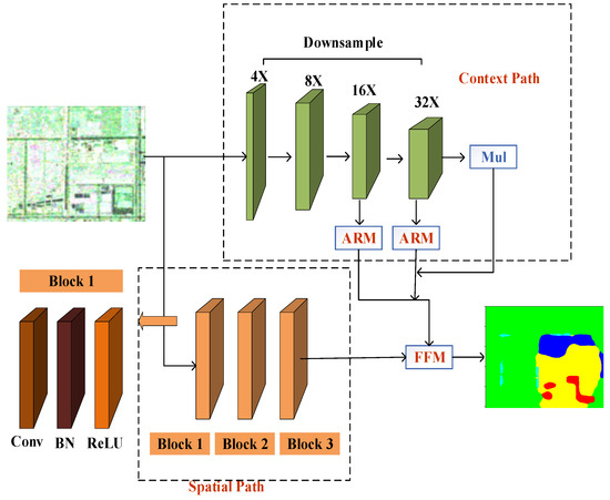
Figure 1.
LoSARNet architecture. Mul represents multiplication operation. Block 1 is composed with Conv, BN and ReLU.
2.1. Improved Loss Function
In the task of SAR image semantic segmentation, the goal is to classify each pixel into an object class. To enable the training of the segmentation model, a loss function is adopted to calculate the loss and continue the back-propagation. The commonly used loss function in image segmentation methods is the CE loss function, which is designed for optimizing the pixel classification accuracy of segmentation results. The CE loss function is expressed in Equation (1).
where is the number of total pixels, represents the true class label of pixel , represents the predicted result of the network for pixel , and represents all outputs of the network. This means that the non-standardized output of the network has been mapped to the probability space by a softmax unit, as shown in Equation (2).
where represents the total categories of the segmentation task. CE helps the network smoothly optimize the loss function, which is usually tested by using the category with the highest score as the final predictor of the pixels, i.e., .
While the CE loss function is commonly used to optimize the loss curve in a semantic segmentation task, it is not the primary index for evaluating the performance of a semantic segmentation task. In practical scenarios, the Jaccard index, also known as the IOU score, is employed to assess the accuracy of semantic segmentation tasks. Given the ground-truth tag vector and the prediction tag vector, the Jaccard index of class is defined as Equation (3):
The Jaccard index quantifies the level of agreement between the network output and the ground truth, serving as a reliable measure to evaluate the performance of a semantic segmentation network. Hence, the Jaccard index has more reliability than does cross-entropy loss. To optimize the network towards maximizing the IOU score, the minimization of the Jaccard loss, as depicted in Equation (4), is considered a reasonable objective.
The IOU is a discrete, non-differentiable metric, while the outputs of the network are continuous. And discretization will result in non-differentiable situation. As a result, the Jaccard loss cannot be used for loss optimization directly. The Lovász extension is proposed by Berman et al. [39] to make the Jaccard loss differentiable and convert the input value from discrete to continuous . The output value of the convex surrogate loss functions is equal to the output value of the original function in , which has the properties of a convex function, so it maintains a consistent optimization direction. After the Lovász extension, the formula for the Lovász-softmax function of the Jaccard loss can be defined as follows:
where represents loss surrogate of Jaccard loss and represents pixel errors, and is used to construct the convex surrogate of . represents the true classification value of a pixel, represents the prediction of the network for the pixel , is a subclass of , and is the multiclass.
In practice, the IOU index is sensitive to hyper-parameters such as learning rates and batch sizes. Considering this situation, the training process is divided into two stages; cross-entropy loss is first used to make hyper-parameters converge toward optimal values. And in the second stage, which called the fine-tuning stage, the Lovász-softmax loss is used in order to achieve better prediction accuracy. The loss function utilized in the paper can be described by Equation (6):
where is the number of pixels, represents the network’s probability for pixel , means loss surrogate, and represents pixel errors. The staged loss function is more suitable for the optimization process of the network.
2.2. Architecture of LoSARNet
2.2.1. Spatial Path (SP) and Context Path (CP)
In order to generate a high-quality predicted result, dilated convolution is utilized in [34] to prevent the loss of resolution in the output image by inserting holes between elements. A pyramid pooling module [44] and spatial pyramid pooling [45] are proposed to capture a sufficient receptive field. This reveals that the spatial information and the receptive field are essential issues for reaching high levels of accuracy, even though it is difficult to achieve them at the same time. In the context of semantic segmentation tasks on PolSAR images, image splitting and lightweight networks are frequently adopted to accelerate real-time semantic segmentation [37]. The split operation will disrupt the spatial continuity of the input map, and the channel pruning used in shallow networks will also damage the spatial information between channels. This runs counter to the full use of information. Based on this observation, a network structure with a small number of convolution layers is adopted to obtain spatial information, and named SP. The SP can encode affluent spatial information while maintaining a feature map 1/8 the size of the original input image. It consists of three blocks, as shown in Figure 1. Each block is composed of a convolution layer with parameters [stride = 2, kernel size = 3, and padding = 1], a BN layer, and a ReLU layer. The convolution layer extracts the low-layer features of the image through the convolution operations with the convolution kernel; the batch normalization layer standardizes the output of the convolution layer, controlling the gradient explosion to prevent the gradient from disappearing, and prevents overfitting; the ReLU layer introduces nonlinear features to strengthen the feature-learning ability of the network.
Except for the attention on the spatial information, the acquisition of context information is also of great importance for segmentation results. Enlarging the receptive field and fusing different forms of context information are the most-used methods to obtain enough context information. To expand the receive field, some networks use pyramid pooling, jumper connections [46], and dilated convolution [47]. However, these methods require larger computation memory, resulting in slower segmentation speeds [37]. When dealing with PolSAR images, large receptive fields and efficient computation must be considered. To achieve this, the ResNet18 network is designed as the CP. The ResNet18 contains 17 convolution layers and a fully connected layer. The CP is shown in Figure 1, which removes the fully connected layer. Thus, the CP takes advantage of the lighter model to achieve fast down-sampling, obtain a larger receive field and encode high-level context information while maintaining speed. Additionally, global averaging pooling is used at the end of CP to provide global context information for the receptive field. In practice, the lightweight ResNet18 network is used for multiple down-sample steps to obtain considerable receptive field attainment and finally, the output feature map and the global pooling output of ResNet18 are combined.
2.2.2. Attention Refinement Module (ARM) and Feature Fusion Module (FFM)
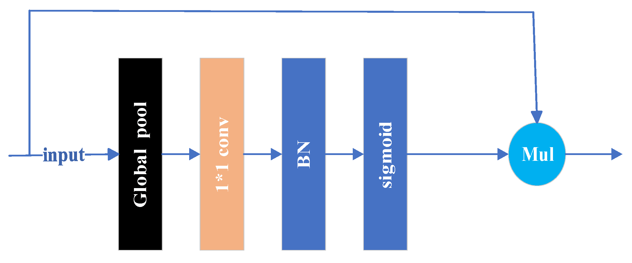
The ARM illustrated in Figure 2 is placed in the CP, following the 16x down-sampling module and the 32× down-sampling module. The input of ARM is the original feature map obtained after down-sampling. The ARM module is used to refine the characteristics of each stage. The ARM structure consists of a global pooling module, a 1 × 1 convolution operation, a BN layer, and a sigmoid function. The global pooling is used to obtain global context information, as well as for squeezing length and width, and retaining the channel information; the 1 × 1 convolution is adopted for integrating cross-channel feature information and reducing parameters of convolutional kernel; the BN layer is exploited to normalize the input features; the sigmoid function is utilized to activate and introduce more nonlinear features, in order to reinforce the ability of feature expression and normalize the feature weights to [0,1]. Finally, matrix multiplication is employed to multiply the normalized weight matrix with the original features to obtain attention-enhanced features.

Figure 2.
ARM architecture.
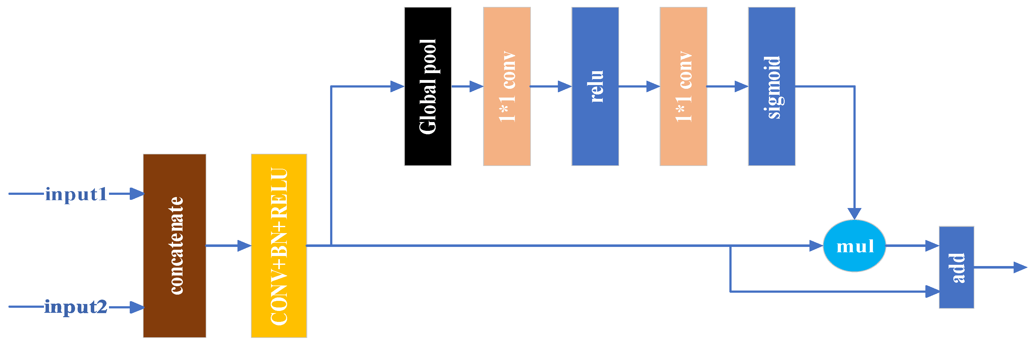
Due to the different feature functions of the SP and the CP, the feature maps obtained from the two paths also have different levels of representation. The SP encodes the main spatial detail information, which has low-level features. And, the CP encodes the context information, which is composed of high-level features. It is not suitable to simply add the feature maps of the two paths. Therefore, the outputs of the CP and the SP are used as the input of the FFM, which is employed to fuse the features correctly. Firstly, the FFM module combines the low-level SP output and the high-level CP output, and then the BN layer is used for hierarchical normalization. Finally, the global pooling module is used to calculate the weight vector for selecting and combing the features. By multiplying the obtained weight vector, layer by layer, onto the original feature map, the channel dimension rescaling is completed. The structure of the FFM is shown in Figure 3, which has a similar structure to that of the ARM, except the feature-fusing part.

Figure 3.
FFM architecture.
3. Datasets and Pre-Processing
To verify the effectiveness of the proposed LoSARNet, the experimental datasets are introduced in this section, including the AIR-PolSAR-Seg data, the classical Flevoland data and the Oberpfaffenhofen data. Then, the pre-processing of the experimental data is given. Finally, the evaluation metrics for segmentation performance analysis are listed.
3.1. Datasets
- (1)
- AIR-PolSAR-Seg data [43]: The AIR-PolSAR-Seg data supplies the PolSAR amplitude images captured by the Gaofen-3 satellite in quad-polarized strip I (QPSI) mode on 29 April 2019. The PolSAR amplitude images include four polarization modes, viz., vertical–vertical (VV), horizontal–vertical (HV), horizontal–horizontal (HH), and vertical–horizontal (VH). The spatial resolution of the images is 8 m, and it is annotated with respect to six typical terrain categories at the pixel level, including housing areas, industrial areas, natural areas, land-use areas, water areas, and other areas. Figure 4 exhibits the PolSAR amplitude image under an HH polarization state and the corresponding ground-truth map with color codes.
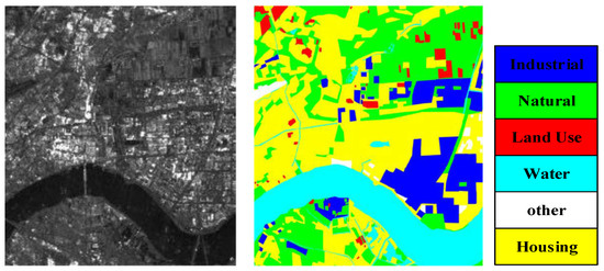 Figure 4. AIR-PolSAR-Seg data source: amplitude image and the ground truth with color codes.
The PolSAR image annotation is well performed by researchers in AIRCAS. A radiation calibration operation is conducted to suppress speckle noise, and the ground truth is labeled by Wang et al. manually [43]. And the PolSAR image of AIR-PolSAR-Seg is cropped into 500 patches with a size of 512 × 512. Since each PolSAR image patch contains four polarization modes, the total number of PolSAR image patches is 2000 (500 × 4). And the PolSAR amplitude images of HH, HV, VH, and VV are all real numbers.
- (2)
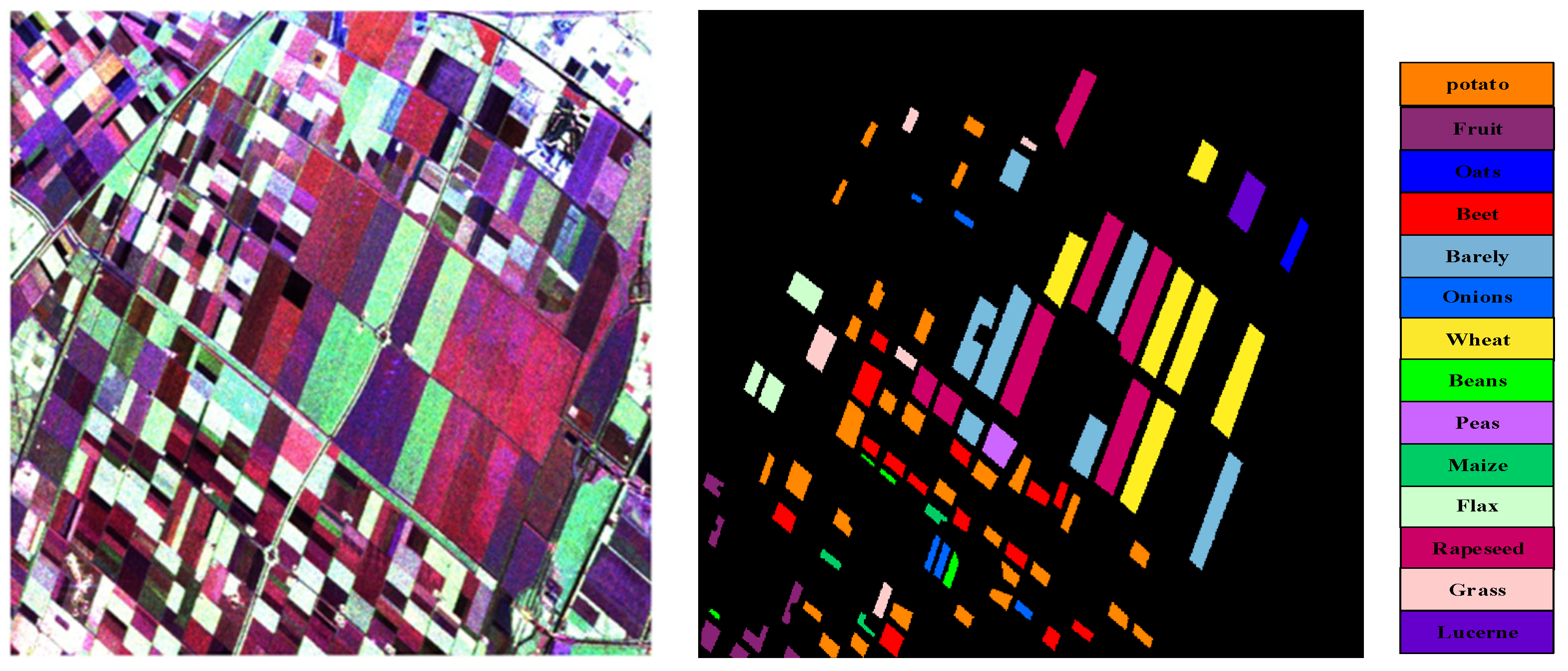
- Flevoland data: The Flevoland data here was acquired by NASA/JPL AIRSAR in 1991, and is widely used in many research efforts regarding PolSAR image classification [15,19,23,24,42]. The size of the PolSAR image is 1020 × 1024, with a spatial resolution of 10 m. Figure 5 displays a pseudo-RGB image of the Flevoland area data, which are obtained by Pauli decomposition [3,5,6,7]. As the coherence matrix is obtained, the spatial average operation is employed to suppress the speckle noise. The ground-truth class labels and color codes are also given in Figure 5, where the black regions are regarded as the background. The Flevoland area dataset includes 14 categories, namely, Potato, Fruit, Oats, Beet, Barley, Onions, Wheat, Beans, Peas, Maize, Flax, Rapeseed, Grass, and Lucerne, respectively.
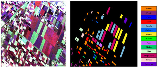 Figure 5. Flevoland data: Pauli pseudo-RGB image and the ground truth with color codes.
 - (3)
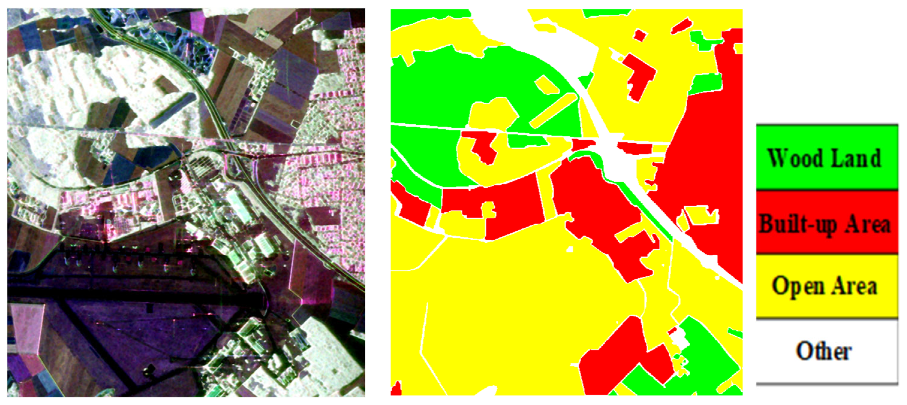
- Oberpfaffenhofen data: The Oberpfaffenhofen data set was acquired by E-SAR. It is widely used in much research relevant to PolSAR image classification [19,43]. The data is acquired in L-band and has been multi-looked. The size of the PolSAR image is 1300 × 1200 pixels, and the spatial resolution is 3 m. The Pauli image and the ground truth are shown in Figure 6. In Figure 6, the ground-truth class labels cover four typical terrain categories, including Built-up Area, Wood Land, Open Area, and Other.
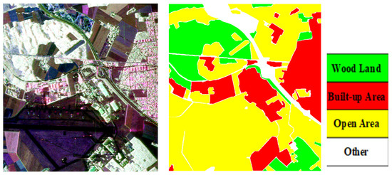 Figure 6. Oberpfaffenhofen data: Pauli pseudo-RGB image and the ground truth with color codes.
3.2. Pre-Processing and Training
The PolSAR image data consists of multiple polarization channels. Thus, it is necessary to perform a normalization operation to avoid an imbalanced initialization of weights. The input of LoSARNet is first normalized with the batch normalization layer, and the data augmentation is applied by random cropping, horizontal flipping, and vertical flipping.
For optimization, the AdamW optimizer [48] is used for 200 epochs. The learning rate starts from 0.0001, and the l2-norm regularization is employed, with a weight decay of 0.01 to avoid overfitting. To achieve a better training result, the dynamic learning rate adjustment strategy is adopted to optimize the loss of validation set. The specific strategy is that the learning rate will be decreased to 0.7 times the current learning rate after the 11th epoch, if no validation loss decrease is detected within 10 epochs and no improvement occurs in the 11th epoch. Additionally, the minimum learning rate is set as 10−7 to prevent the low learning rate from causing a slow optimization speed.
After training for 200 epochs, the weight with best performance on the validation set is chosen to be the network weight to continue the next stage. During the fine-tuning stage, the pre-trained network is optimized with the Lovász-softmax loss function and cross-entropy loss function as given in Equation (6). Notably, during training, the two outputs of the context path behind the ARMs are used as the auxiliary loss functions [37]. Table 1 summarizes the key training parameters and algorithms in different training stages.

Table 1.
Training parameter settings.
During the training process, the early-stopping policy is utilized. The patience is set as 20, which means a network with optimal generalization performance is obtained if the validation loss no longer drops within 20 epochs. During the testing process, the test image is normalized at first and input into the trained network. After ‘softmax’ operation on the output, the category with the highest scoring class value is assigned to the pixel.
3.3. Evaluation Metrics
The experiments are evaluated using the accuracy for each scene in the dataset. Four metrics are used to evaluate the segmentation performance of the proposed network, including the mean pixel accuracy (MPA), overall accuracy (OA), mean IOU (MIOU), and Kappa coefficient.
where indicates pixels which belong to class but are predicted to be class , and indicates the categories in total. MPA and OA measure the pixel-accuracy of classification. MIOU and Kappa coefficient are used to measure the overall segmentation effect.
4. Experiments
In this section, experiments are performed on the aforementioned datasets. In order to verify the segmentation performance of the proposed LoSARNet, some typical semantic segmentation networks, including ENetV2, ERFNet, DeepLabV3 and BiSeNet, are mentioned for comparisons. The experiments are all performed on a PC with Intel Xeon Platinum 8269CY CPU (Intel, Santa Clara, CA, USA), 128GB RAM, and a NVIDA GeForce RTX3080 GPU (NVIDA, Santa Clara, CA, USA).
4.1. AIR-PolSAR-Seg
As introduced in Section 3.1, the AIR-PolSAR-Seg dataset contains 2000 PolSAR amplitude image patches in total. In the experiment, the training samples are 1400 (350 × 4), and the validation samples are 200 (50 × 4); the remaining 400 (100 × 4) PolSAR image patches are set as test samples.
Since the AIR-PolSAR-Seg dataset supplies the amplitude patch data under four polarizations, HH, HV, VH, and VV, the four-channel PolSAR images are accordingly used as the input of LoSARNet. As shown in Figure 4, six effective categories are considered during the input processing. As only the cropped 512×512 patch amplitude data is obtained from AIR-PolSAR-Seg, the patch PolSAR amplitude images are taken to obtain the segmentation results and the subsequent semantic segmentation indices. Then, the training data is converted into a 4-D tensor with the dimensions of 350 × 512 × 512 × 4 as input to train the architecture of LoSARNet, which represents 350 × 4 PolSAR images extracted from the original dataset as training data. Each image has 512×512 pixels of a spatial dimension and four channels corresponding to the amplitude values achieved under the four polarization modes.
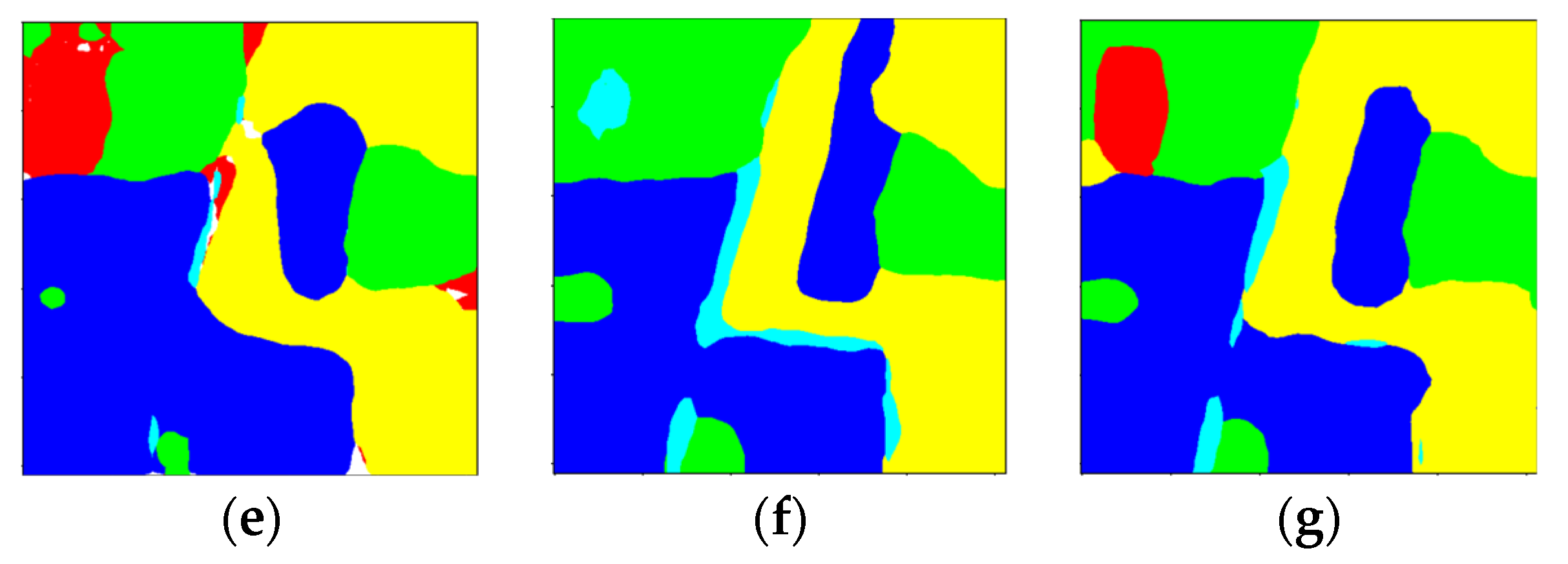
To validate the performance of the loss function used and the improvement of LoSARNet compared to BiSeNet, the results of the two networks with the same training algorithm for the AIR-PolSAR-Seg dataset are shown in Figure 7. A 512 × 512 PolSAR patch image is used for the vision-based illustration. Figure 7a is the pseudo-RGB image of the example patch A. As the AIR-PolSAR-Seg dataset supplies amplitude data under different polarizations, the pseudo-RGB image here is composed by R = |HH|, G = |HV|, and B = |VV|. Figure 7b shows the ground truth of patch A, and Figure 7c displays the segmentation results by using BiSeNet, which adopts the cross-entropy loss function. For regions with small distribution, such as the red and cyan areas, the feature map obtained from the space path is only 1/8 of the size of the original map, and the network trained in cross-entropy can only with difficulty correctly identify these objects, resulting in poor classification results. Figure 7d represents the segmentation results achieved using the proposed LoSARNet. By using the improved loss function as expressed in Equation (6) to jointly optimize the training results, more precise segmentation results are obtained. This validates the proposition that the gaps in the partition can be filled by the loss function to have a better performance in the unevenly distributed dataset. It has a particular advantage in recovering small objects, allowing for more comprehensive segmentation results.

Figure 7.
The patch (A) used for comparison: (a) pseudo-RGB image of patch A; (b) ground truth of patch A; (c) patch A segmentation result using BiSeNet; (d) patch A segmentation result using LoSARNet.
To verify the performance of LoSARNet further, it is compared to BiSeNet networks trained with different loss functions, and multiple other networks. All the experiments are conducted using the same training data, data augmentation approach, and dynamic learning rate strategy, in which Xception is used in DeepLabV3 as the backbone network. The dynamic learning rate strategy mentioned in Section 3.2 is applied and has obtained a network with optimal generalization performance in rounds of 200. For proper accuracy assessment, the training and test sets used in this paper do not overlap.
Quantitative analysis of the metrics for the AIR-PolSAR-Seg by BiSeNet with different loss functions are shown in Table 2. As mentioned in Section 3.2, the two outputs of the context path behind the ARMs are used as the auxiliary loss functions. In BiSeNet, all three outputs use cross-entropy to optimize three loss functions. 1-Lovász denotes that the Lovász-softmax loss function is only used in the main output of the network, while 3-Lovász takes all three outputs for Lovász-softmax to optimize three loss functions. The proposed loss function introduced in Equation (6) is employed for LoSARNet. In Table 2, it is obvious that the MIOU of LoSARNet (51.50%) is higher than that of BiSeNet (42.66%). And the other two results also have higher MIOU than BiSeNet, which means the Lovász-softmax loss function can improve MIOU. The OA and Kappa of LoSARNet provide the highest results. This reveals the advantage of LoSARNet. A noteworthy issue is that the result of BiSeNet has higher OA and lower MPA compared to other results. This is because the network focuses more on categories with a larger proportion and is less sensitive to categories with a smaller proportion. And the Lovász-softmax loss function helps the network pay attention to the regional features of the image, which can also have good effects on small classes. However, using only the Lovász-softmax loss function will focus too much on small categories, resulting in suboptimal overall network results. LoSARnet clearly balances pixel accuracy and overall segmentation performance, and the improvements show the effectiveness of the proposed loss function strategy.

Table 2.
The metric values for AIR-PolSAR-Seg by different loss functions.
Segmentation results of AIR-PolSAR-Seg obtained by different networks are shown in Figure 8 by taking one patch as an illustration example. From a visual perspective, EnetV2, ERFNet, and DeepLabV3 have misclassified pixels and are unable to correctly identify bare ground and river areas. In Figure 8c, the ENetV2 network fails to learn image features correctly, resulting in blurry areas in the segmentation result. The best segmentation results are achieved by the proposed LoSARNet. The BiSeNet network incorrectly classifies the bare ground area in the upper left corner of the image, which incorrectly predicts most of the naked pixels in red color as rivers in cyan color. In contrast, LoSARNet correctly classifies the bare ground area and obtains a more ideal segmentation result.

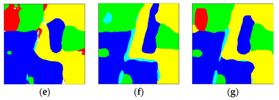
Figure 8.
Results with different semantic networks for comparison: (a) pseudo-RGB image of the example patch; (b) ground truth; (c) ENetV2 segmentation result; (d) ERFNet segmentation result; (e) DeepLabV3 segmentation result; (f) BiSeNet segmentation result; (g) LoSARNet segmentation result.
Quantitative analysis of the metrics for the AIR-PolSAR-Seg by different networks is shown in Table 3. It can be seen from Table 3 that the MPA, OA, MIOU, and Kappa evaluations of LoSARNet are far superior to the other methods, especially the MIOU. LoSARNet obtains an MIOU of 51.50%, which is higher than that of ERFNet, with 48.15%; ENetV2, with 43.36%; and DeepLabV3, with 40.42%. ENetV2, ERFNet, and LoSARNet all perform strongly on the Kappa coefficient, which means better overall segmentation performance. For pixel accuracy, LoSARNet achieved the best results on MPA and OA, and had a significant improvement in effectiveness. At the same time, LoSARNet possesses the highest recognition speed, surpassing the two real-time semantic segmentation networks ENetV2 and ERFNet.

Table 3.
The metric values for AIR-PolSAR-Seg by different segmentation networks.
4.2. Flevoland
As introduced in Section 3.1, the complete PolSAR image is sized 1020×1024. Different from Pol-AIRSAR-Seg data, the Flevoland data provides a complete polarimetric coherence matrix. A window of size 256 × 256 slides over the PolSAR image with steps of 32 to finally obtain the 625 PolSAR patch images in total, each with a size of 256×256 in six channels. And the six channels correspond to the polarimetric coherence matrix [3] elements, which are T11, T12, T13, T22, T23, and T33. A total of 10% of the data is used as the training set, 20% as the verification set, and the rest is used for the test set; each patch dataset has a size of 256 × 256 × 6. According to the research in [9], the 6-D complex-valued matrix is converted into a 6D real-valued vector based on the consideration of the elements of the coherence matrix.
where SPAN is the total intensity and equals ; A represents the total power of all channels (dB); B and C are normalized channel values of T22 and T33. D, E, F are relative correlation coefficients.
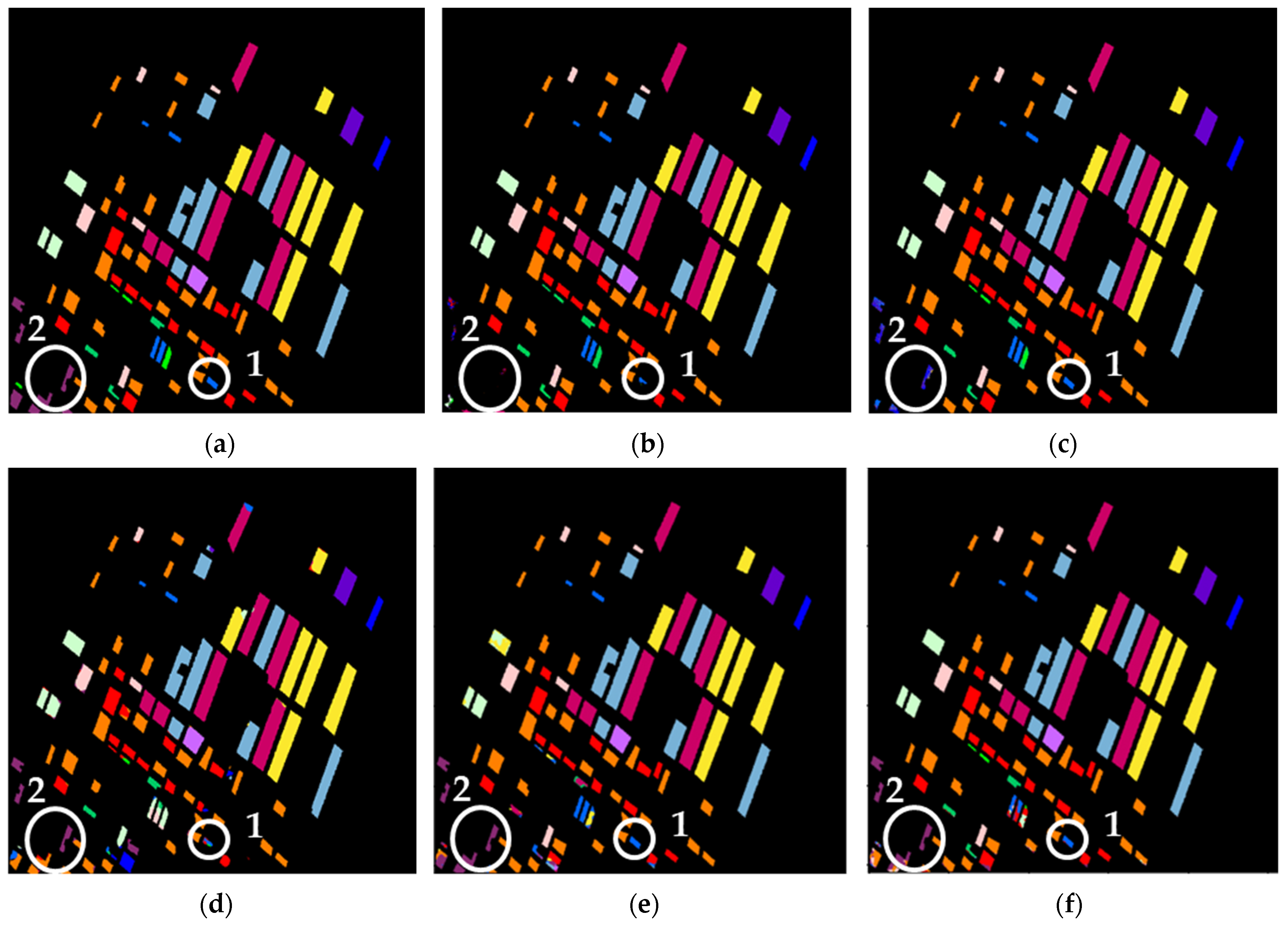
Through the comparison and analysis of the experiment in Section 4.1, the LoSARNet shows great superiority to other networks on complex large scenes. The Flevoland data includes 14 categories, posing new challenges for the segmentation. The experiment’s results are shown in Figure 9. In marked area 1, the results of ERFNet and LoSARNet demonstrate consistency with the ground-truth map. DeepLabV3 misclassifies the class Oats, and ENetV2 clearly cannot distinguish this class from the background, although the weight of the background is set very low in the experiment. In marked area 2, the correct category is Fruit, and only BiSeNet and LoSARNet classify most pixels correctly. The quantitative comparison is given in Table 4. The semantic segmentation metrics obtained by LoSARNet are better than those of other networks. For MIOU, the performance of LoSARNet is 86.06%, which is higher than that of BiSeNet, 79.01%. The improvement is very huge. ENetV2 and ERFNet also perform well in IOU with 81.34% and 84.78%, respectively. For MPA, LoSARNet also has an improvement of about 7 percentage points compared with BiSeNet. And as for OA and Kappa, all networks achieve good results. The above results show that the proposed LoSARNet can effectively extract the features of PolSAR image features with better segmentation accuracy.
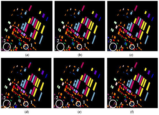
Figure 9.
The segmentation results of Flevoland data: (a) ground-truth map; (b) ENetV2; (c) ERFNet; (d) DeepLabV3; (e) BiSeNet; (f) LoSARNet.

Table 4.
The metric values for Flevoland by BiSeNet and LoSARNet.
The application of LoSARNet in the segmentation of Flevoland data has been proved to extract features and classify the PolSAR images effectively. LoSARNet achieves better segmentation results than do other networks, which is supported by the IOU score for Flevoland, as shown in Table 5. It is obvious that LoSARNet is completely superior to BiSeNet. Additionally, it can be noticed that the results of ENetV2 and ERFNet are also very good. However, the recognition of certain categories is almost completely incorrect, which is usually difficult to accept in most segmentation tasks. Although LoSARNet achieved nearly 100% accuracy in most categories, slightly lower than EnetV2 and ERFNet, it still ensured accuracy in most categories.

Table 5.
The IOU scores of each category for Flevoland.
4.3. Oberpfaffenhofen
As introduced in Section 3.1, the complete PolSAR image has a size of 1300 × 1200, and hence, a window of size 256 × 256 slides over the PolSAR image with steps of 32 to finally obtain the 1054 PolSAR patch images in total with the size of 256 × 256, in six channels. In this experiment, 10% of the samples are set as training set, 10% of samples are set as a validation set, and the rest are used as the test set. The channels of the PolSAR image used in the experiment are the same as those of the Flevoland data, which makes the data real-valued as to vectors.
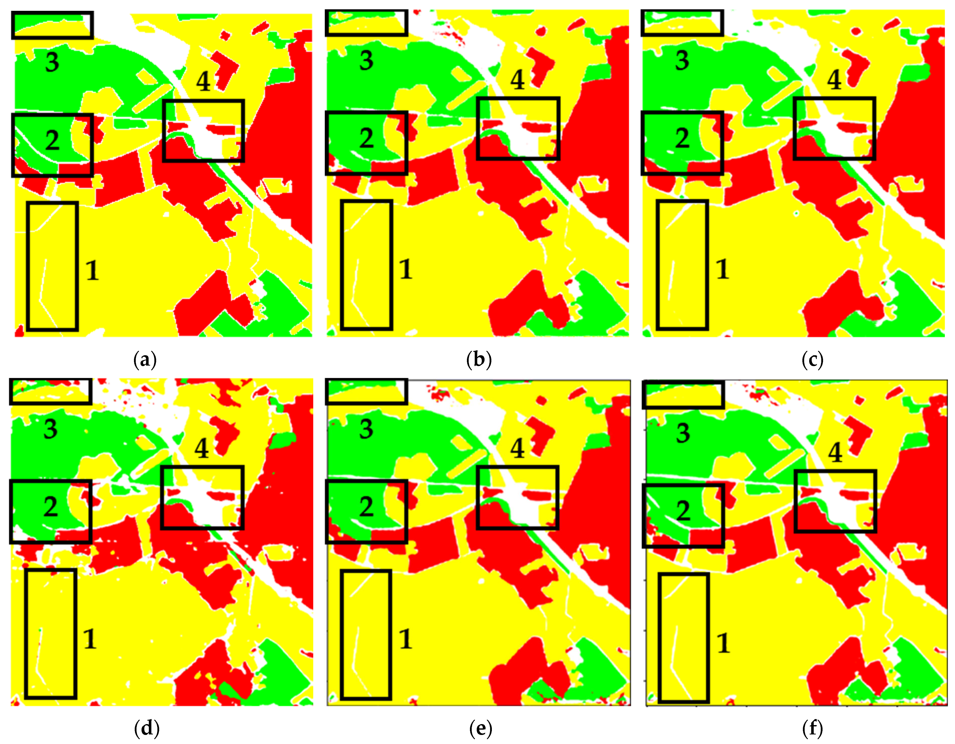
The results for the whole dataset are shown in Figure 10. In marked area 1 and area 2, LoSARNet better preserves the edge information in the ground-truth map compared to other results. BiSeNet has also achieved good results, which may be an advantage brought by bilateral networks. In marked area 3, the misclassification area of LoSARNet is obviously smaller. In marked area 4, the results of LoSARNet are closest to those of the ground-truth map. Considering that all the results are visually good, further attention is focused on the specific quantitative results. All the results are shown in Table 6, and the IOU scores of different categories are given in Table 7. In Table 6, LoSARNet performs best in all evaluation metrics. Specifically, the MIOU of LoSARNet is 94.57%, higher than 88.46%, 86.21%, 71.29%, and 91.19%. Comparing these results with BiSeNet, which already produces good results of 91.19%, a 3.38% increase is remarkable. For MPA, OA, and Kappa, the results of LoSARNet are all above 97%, which means that the segmentation task is almost perfectly completed. The results of other methods are also very good. But there is still a significant gap compared to LoSARNet. In further analyses of IOU scores, LoSARNet achieves the best results for all categories, especially for the category Other; other methods have significant errors, but LoSARNet can distinguish them more accurately. This corresponds to the white area in Figure 10, and we also achieve the same results visually. LoSARNet achieves a huge improvement in IOU. This improvement comes from a more accurate classification of other categories.
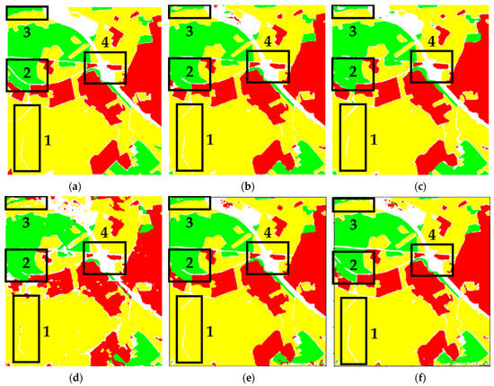
Figure 10.
The segmentation results of Oberpfaffenhofen data: (a) ground-truth map; (b) ENetV2; (c) ERFNet; (d) DeepLabV3; (e) BiSeNet; (f) LoSARNet.

Table 6.
The metric values for Oberpfaffenhofen.

Table 7.
The IOU scores of each category for Oberpfaffenhofen.
5. Discussion
In this paper, LoSARNet is proposed for PolSAR data segmentation. By leveraging a bilateral structure, LoSARNet excels at extracting features efficiently, thereby ensuring both high-speed performance and precise semantic segmentation. To further enhance its segmentation capability, we employ a new loss function that combines the Lovász-softmax loss and CE (cross-entropy) loss within LoSARNet. This joint loss function enables the network to optimize both pixel accuracy and IOU scores simultaneously. As a result, LoSARNet outperforms other existing networks in terms of performance.
To evaluate the segmentation performance of LoSARNet, we conduct experiments on three widely used sets of PolSAR data. These datasets cover various segmentation cases, including complex large scenes, multiple categories, and high-resolution images, each corresponding to different segmentation requirements. Meanwhile, several typical semantic segmentation networks, including ENetV2, ERFNet, DeepLabV3 and BiSeNet, are employed for comparisons. In the case of the AIR-PolSAR-Seg dataset, LoSARNet achieves significantly higher MIOU scores compared to the aforementioned networks, with improvements of 8.14%, 3.35%, 11.08%, and 8.84%. Similarly, the MPA of LoSARNet is higher by 8.16%, 3.50%, 9.89%, and 9.33%, respectively. These experimental results provide strong evidence for the superior performance of LoSARNet. For the Flevoland dataset, the phase information of the network is maximized by converting the six-channel complex-valued data to the six-channel real-valued data. Both LoSARNet and ERFNet achieve good results on this dataset. LoSARNet achieves the best results on MPA, MIOU and Kapp. This confirms the effectiveness of LoSARNet in multi-class segmentation tasks. In the case of the Oberpfaffenhofen dataset, LoSARNet demonstrates its capability in detailed classification of high-resolution PolSAR images. LoSARNet achieves over 90% accuracy for all classification indicators, highlighting its effectiveness. When compared to BiSeNet, LoSARNet achieves improvements of 3.01% and 3.38% in terms of MPA and MIOU, respectively, which are substantial enhancements over the baseline results.
Overall, LoSARNet exhibits superior performance across three PolSAR datasets. These improvements are attributed to the efficient feature extraction enabled by the bilateral structure and the simultaneous optimization of pixel accuracy and IOU through the new loss function.
6. Conclusions
Motivated by the successful application of deep learning methods in PolSAR segmentation, this paper presents a novel SAR network called LoSARNet, which utilizes the Lovász-softmax loss optimization. The network demonstrates exceptional performance compared to other networks when evaluated on various PolSAR datasets, including AIR-PolSAR-Seg, Flevoland, and Oberpfaffenhofen. Considering the disparity between the cross-entropy loss and the segmentation task, this paper proposes an improved loss function and a corresponding two-stage training method. This improved loss function combines Lovász-softmax loss and CE loss to achieve both segmentation performance and pixel accuracy. These improvements help the network to achieve a better result. During the training process, the dynamic learning rate strategy and the early-stopping strategy are employed to accelerate the loss-convergence speed while keeping the loss-function curve from entering the local optimal point. In the comparison to BiSeNet, which also incorporates a dual-path structure, the proposed LoSARNet achieves higher evaluation metrics for all datasets. Meanwhile, LoSARNet has also demonstrated comprehensive, leading performance compared to several other segmentation networks, including ENetV2, ERFNet, and DeepLabV3. The improved loss function in this paper can effectively fill the gaps in the split and obtain more comprehensive segmentation results. Especially when dealing with images containing unevenly distributed data types, the potential of LoSARNet is demonstrable. Overall, this work validates a semantic segmentation network with an improved loss function on three classical PolSAR datasets. To consider the phase information contained in PolSAR data, the complex-valued LoSARNet will be further studied in future research.
Author Contributions
Conceptualization, R.G.; methodology, R.G., X.Z. and G.Z.; validation, X.Z. and G.Z.; formal analysis, Y.W.; resources, Y.L.; writing—original draft preparation, X.Z. and G.Z.; writing—review and editing, R.G. and X.Z. All authors have read and agreed to the published version of the manuscript.
Funding
This work was supported by the State Key Laboratory of Geo-Information Engineering (SKLGIE2020-M-4-2), and the National Natural Science Foundation of China (61971326).
Acknowledgments
The authors would like to thank AIRCAS, Journal of Radars (China), NASA/ Jet Propulsion Laboratory, and the German Aerospace Center for providing the dataset used in the paper.
Conflicts of Interest
The authors declare no conflict of interest.
Abbreviations
| ARM | Attention refinement module |
| BiSeNet | Bilateral segmentation network |
| BN | Batch normalization |
| CE | Cross entropy |
| CNN | Convolutional neural network |
| CP | Context path |
| ERFNet | Efficient residual factorized network |
| FFM | Feature fusion module |
| IOU | Intersection over union |
| LoSARNet | Lovász-softmax loss optimization SAR net |
| MIOU | Mean intersection over union |
| MPA | Mean pixel accuracy |
| OA | Overall accuracy |
| PolSAR | Polarimetric synthetic aperture radar |
| SAR | Synthetic aperture radar |
| SP | Spatial path |
References
- Cumming, I.G.; Wong, F.H. Digital Processing of Synthetic Aperture Data: Algorithms and Implementation; Artech House Remote Sensing Library: Boston, MA, USA, 2005. [Google Scholar]
- Iervolino, P.; Guida, R.; Lumsdon, P.; Janoth, J.; Clift, M.; Minchella, A.; Bianco, P. Ship detection in SAR imagery: A comparison study. In Proceedings of the 2017 IEEE International Geoscience and Remote Sensing Symposium (2017 IGARSS), Fort Worth, TX, USA, 23–28 July 2017. [Google Scholar]
- Yamaguchi, Y. Disaster monitoring by fully polarimetric SAR data acquired with ALOS-PALSAR. Proc. IEEE 2012, 100, 2851–2860. [Google Scholar] [CrossRef]
- Li, W.; Zou, B.; Zhang, L. Ship detection in a large scene SAR image using image uniformity description factor. In Proceedings of the 2017 SAR in Big Data Era: Models, Methods and Applications (BIGSARDATA), Beijing, China, 13–14 November 2017. [Google Scholar]
- Chen, S.; Wang, X.; Sato, M. Urban damage level mapping based on scattering mechanism investigation using fully polarimetric SAR data for the 3.11 East Japan earthquake. IEEE Trans. Geosci. Remote Sens. 2016, 54, 6910–6929. [Google Scholar]
- Praks, J.; Hallikainen, M.; Koeniguer, E.C. Polarimetric SAR image visualization and interpretation with covariance matrix invariants. In Proceedings of the 2017 IEEE International Geoscience and Remote Sensing Symposium-IGARSS 2017 IGARSS, Fort Worth, TX, USA, 23–28 July 2017. [Google Scholar]
- Chen, S.; Li, Y.; Wang, X.; Xiao, S. Polarimetric SAR target scattering interpretation in rotation domain: Theory and application. J. Radars 2017, 6, 442–455. [Google Scholar]
- Henry, C.; Azimi, S.M.; Merkle, N. Road segmentation in SAR satellite images with deep fully convolutional neural networks. IEEE Geosci. Remote Sens. Lett. 2018, 15, 1867–1871. [Google Scholar] [CrossRef]
- Gamba, P.; Aldrighi, M. SAR data classification of urban areas by means of segmentation techniques and ancillary optical data. IEEE J. Sel. Top. Appl. Earth Obs. Remote Sens. 2012, 5, 1140–1148. [Google Scholar] [CrossRef]
- Chatterjee, A.; Saha, J.; Mukherjee, J.; Aikat, S.; Misra, A. Unsupervised land cover classification of hybrid and dual-polarized images using deep convolutional neural network. IEEE Geosci. Remote Sens. Lett. 2021, 18, 969–973. [Google Scholar] [CrossRef]
- Samadi, F.; Akbarizadeh, G.; Kaabi, H. Change detection in SAR images using deep belief network: A new training approach based on morphological images. IET Image Process. 2019, 13, 2255–2264. [Google Scholar] [CrossRef]
- Akbarizadeh, G.; Rezai-Rad, G.; Shokouhi, S. A new Region-Based active contour model with skewness wavelet energy for segmentation of SAR images. IEICE Trans. Inf. Syst. 2010, 93, 1690–1699. [Google Scholar] [CrossRef]
- Akbarizadeh, G. A new statistical-based kurtosis wavelet energy feature for texture recognition of SAR images. IEEE Trans. Geosci. Remote Sens. 2012, 50, 4358–4368. [Google Scholar] [CrossRef]
- Tirandaz, Z.; Akbarizadeh, G.; Kaabi, H. PolSAR image segmentation based on feature extraction and data compression using weighted neighborhood filter bank and hidden Markov random field-expectation maximization. Measurement 2020, 153, 107432. [Google Scholar] [CrossRef]
- Yu, L.; Zeng, Z.; Liu, A.; Xie, X.; Wang, H.; Xu, F.; Hong, W. A lightweight complex-valued DeepLabv3+ for semantic segmentation of PolSAR image. IEEE J. Sel. Top. Appl. Earth Obs. Remote Sens. 2022, 15, 930–943. [Google Scholar] [CrossRef]
- Krizhevsky, A.; Sutskever, I.; Hinton, G.E. Imagenet classification with deep convolutional neural networks. Adv. Neural Inf. Process. Syst. 2012, 25, 1–9. [Google Scholar] [CrossRef]
- Malmgren-Hansen, D.; Nobel, J.M. Convolutional neural networks for SAR image segmentation. In Proceedings of the 2015 IEEE International Symposium on Signal Processing and Information Technology (ISSPIT), Abu Dhabi, United Arab Emirates, 7–10 December 2015. [Google Scholar]
- Liu, Y.; Zhang, M.; Xu, P.; Guo, Z. SAR ship detection using sea-land segmentation-based convolutional neural network. In Proceedings of the 2017 International Workshop on Remote Sensing with Intelligent Processing (RSIP), Shanghai, China, 18–21 May 2017. [Google Scholar]
- Zhang, Z.; Wang, H.; Xu, F.; Jin, Y. Complex-valued convolutional neural network and its application in polarimetric SAR image classification. IEEE Trans. Geosci. Remote Sens. 2017, 55, 7177–7188. [Google Scholar] [CrossRef]
- Duan, Y.; Tao, X.; Han, C.; Qin, X.; Lu, J. Multi-scale convolutional neural network for SAR image semantic segmentation. In Proceedings of the 2018 IEEE Global Communications Conference (GLOBECOM), Abu Dhabi, United Arab Emirates, 9–13 December 2018. [Google Scholar]
- Davari, N.; Akbarizadeh, G.; Mashhour, E. Corona detection and power equipment classification based on GoogleNet-AlexNet: An accurate and intelligent defect detection model based on deep learning for power distribution lines. IEEE Trans. Power Deliv. 2021, 37, 2766–2774. [Google Scholar] [CrossRef]
- Sharifzadeh, F.; Akbarizadeh, G.; Seifi, K. Ship classification in SAR images using a new hybrid CNN–MLP classifier. J. Indian Soc. Remote Sens. 2019, 47, 551–562. [Google Scholar] [CrossRef]
- Mullissa, A.G.; Persello, C.; Stein, A. PolSARNet: A deep fully convolutional network for polarimetric SAR image classification. IEEE J. Sel. Top. Appl. Earth Ober. Remote Sens. 2019, 12, 5300–5309. [Google Scholar] [CrossRef]
- Persello, C.; Stein, A. Deep fully convolutional networks for the detection of informal settlements in VHR images. IEEE Geosci. Remote Sens. Lett. 2017, 14, 2325–2329. [Google Scholar] [CrossRef]
- Mohammadimanesh, F.; Salehi, B.; Mahdianpari, M.; Gill, E.; Molinier, M. A new fully convolutional neural network for semantic segmentation of polarimetric SAR imagery in complex land cover ecosystem. ISPRS J. Photogramm. Remote Sens. 2019, 151, 223–236. [Google Scholar] [CrossRef]
- Zhang, C.; Pan, X.; Li, H.; Gardiner, A.; Hare, J.; Atkinson, P.M. A hybrid MLP-CNN classifier for very fine resolution remotely sensed image classification. ISPRS J. Photogramm. Remote Sens. 2018, 140, 133–144. [Google Scholar] [CrossRef]
- Long, J.; Shelhamer, E.; Darrrell, T. Fully convolutional networks for semantic segmentation. IEEE Trans. Pattern Anal. Mach. Intell. 2015, 38, 3431–3440. [Google Scholar]
- Yao, W.; Marmanis, D.; Datcu, M. Semantic Segmentation Using Deep Neural Networks for SAR and Optical Image Pairs; German Aerospace Center (DLR): Koln, Germany, 2017. [Google Scholar]
- Wang, X.; Cavigelli, L.; Eggimann, M.; Magno, M.; Benini, L. HR-SAR-Net: A deep neural network for urban scene segmentation from high-resolution SAR data. In Proceedings of the 2020 IEEE Sensors Applications Symposium (SAS), Kuala Lumpur, Malaysia, 9–11 March 2020. [Google Scholar]
- Paszke, A.; Chaurasia, A.; Kim, S.; Culurciello, E. ENet: A deep neural network architecture for real-time semantic segmentation. arXiv 2016, arXiv:1606.02147. [Google Scholar]
- Wang, Y. Remote sensing image semantic segmentation algorithm based on improved Enet network. Sci. Program. 2021, 2021, 5078731. [Google Scholar] [CrossRef]
- Romera, E.; Alvarez, J.; Bergasa, L.; Arroyo, R. Erfnet: Efficient residual factorized convnet for real-time semantic segmentation. IEEE Trans. Int. Trans. Syst. 2017, 19, 263–272. [Google Scholar] [CrossRef]
- Yin, H.; Zhang, C.; Han, Y.; Qian, Y.; Xu, T.; Zhang, Z.; Kong, A. Improved semantic segmentation method using edge features for winter wheat spatial distribution extraction from Gaofen-2 images. J. Appl. Remote Sens. 2021, 15, 028501. [Google Scholar] [CrossRef]
- Chen, L.; Zhu, Y.; Papandreou, G.; Schroff, F.; Adam, H. Encoder-decoder with atrous separable convolution for semantic image segmentation. In Proceedings of the 15th European Conference on Computer Vision (ECCV), Munich, Germany, 8–14 September 2018. [Google Scholar]
- Balasooriya, N.; Dowden, B.; Chen, J.; Silva, O.D.; Huang, W. In-situ sea ice detection using DeepLabv3 semantic segmentation. In Proceedings of the OCEANS 2021, San Diego, CA, USA, 20–23 September 2021. [Google Scholar]
- Aghaei, N.; Akbarizadeh, G.; Kosarian, A. Osdes_net: Oil spill detection based on efficient_shuffle network using synthetic aperture radar imagery. Geocarto Int. 2022, 37, 13539–13560. [Google Scholar] [CrossRef]
- Yu, C.; Wang, J.; Peng, C.; Gao, C.; Yu, G.; Sang, N. Bisenet: Bilateral segmentation network for real-time semantic segmentation. In Proceedings of the European Conference Computer Vision ECCV, Munich, Germany, 10–13 September 2018. [Google Scholar]
- Dai, M.; Leng, X.; Xiong, B.; Ji, K. Sea-land segmentation method for SAR images based on improved BiSeNet. J. Radars 2020, 9, 886–897. [Google Scholar]
- Berman, M.; Triki, A.; Blaschko, M. The lovász-softmax loss: A tractable surrogate for the optimization of the intersection-over-union measure in neural networks. In Proceedings of the IEEE Conference on Computer Vision and Pattern Recognition, Salt Lake City, UT, USA, 18–22 June 2018. [Google Scholar]
- Goodfellow, I.; Bengio, Y.; Courville, A. Deep Learning; MIT Press: Cambridge, UK, 2016. [Google Scholar]
- Everingham, M.; Winn, J. The PASCAL visual object classes challenge 2012 (VOC2012) development kit. Pattern Anal. Stat. Model. Comput. Learn. Tech. Rep. 2012, 2007, 1–45. [Google Scholar]
- Rakhlin, A.; Davydow, A.; Nikolenko, S. Land cover classification from satellite imagery with u-net and lovász-softmax loss. In Proceedings of the IEEE CCVPRW, Salt Lake City, UT, USA, 18–22 June 2018. [Google Scholar]
- Wang, Z.; Zeng, X.; Yan, Z.; Kang, J.; Sun, X. AIR-PolSAR-Seg: A large-scale data set for terrain segmentation in complex-scene PolSAR images. IEEE J. Sel. Top. Appl. Earth Obs. Remote Sens. 2022, 15, 3830–3841. [Google Scholar] [CrossRef]
- Zhao, H.; Shi, J.; Qi, X.; Wang, X.; Jia, J. Pyramid scene parsing network. In Proceedings of the IEEE Conference Computer Vision and Pattern Recognition, Honoluu, HI, USA, 21–26 July 2017. [Google Scholar]
- He, K.; Zhang, X.; Ren, S.; Sun, J. Spatial pyramid pooling in deep convolutional networks for visual recognition. IEEE Trans. Pattern Anal. Mach. Int. 2015, 37, 1904–1916. [Google Scholar] [CrossRef]
- Ronneberger, O.; Fischer, P.; Brox, T. U-net: Convolutional networks for biomedical image segmentation. In Proceedings of the International Conference Medical Image Computing Computer-Assisted Intervention, Munich, Germany, 5–9 October 2015. [Google Scholar]
- Yu, F.; Koltun, V.; Funkhouser, T. Dilated residual networks. In Proceedings of the IEEE Conference Computer Vision and Pattern Recognition, Honolulu, HI, USA, 21–26 July 2017. [Google Scholar]
- Loshchilov, I.; Hutter, F. Decoupled weight decay regularization. In Proceedings of the 2019 International Conference on Learning Representations (ICLR 2019), New Orleans, LA, USA, 6–9 May 2019. [Google Scholar]
Disclaimer/Publisher’s Note: The statements, opinions and data contained in all publications are solely those of the individual author(s) and contributor(s) and not of MDPI and/or the editor(s). MDPI and/or the editor(s) disclaim responsibility for any injury to people or property resulting from any ideas, methods, instructions or products referred to in the content. |
© 2023 by the authors. Licensee MDPI, Basel, Switzerland. This article is an open access article distributed under the terms and conditions of the Creative Commons Attribution (CC BY) license (https://creativecommons.org/licenses/by/4.0/).


