GLF-Net: A Semantic Segmentation Model Fusing Global and Local Features for High-Resolution Remote Sensing Images

Abstract

Semantic segmentation of high-resolution remote sensing images holds paramount importance in the field of remote sensing. To better excavate and fully fuse the features in high-resolution remote sensing images, this paper introduces a novel Global and Local Feature Fusion Network, abbreviated as GLF-Net, by incorporating the extensive contextual information and refined fine-grained features. The proposed GLF-Net, devised as an encoder–decoder network, employs the powerful ResNet50 as its baseline model. It incorporates two pivotal components within the encoder phase: a Covariance Attention Module (CAM) and a Local Fine-Grained Extraction Module (LFM). And an additional wavelet self-attention module (WST) is integrated into the decoder stage. The CAM effectively extracts the features of different scales from various stages of the ResNet and then encodes them with graph convolutions. In this way, the proposed GLF-Net model can well capture the global contextual information with both universality and consistency. Additionally, the local feature extraction module refines the feature map by encoding the semantic and spatial information, thereby capturing the local fine-grained features in images. Furthermore, the WST maximizes the synergy between the high-frequency and the low-frequency information, facilitating the fusion of global and local features for better performance in semantic segmentation. The effectiveness of the proposed GLF-Net model is validated through experiments conducted on the ISPRS Potsdam and Vaihingen datasets. The results verify that it can greatly improve segmentation accuracy.

1. Introduction

As image processing technology, sensors, and data storage capabilities continue to advance, the acquisition of high-resolution (HR) remote sensing images has become more common and feasible [1]. HR remote sensing images refer to image data with corresponding spatial resolutions acquired by remote sensing platforms, such as satellites, aviation, or unmanned aerial vehicles. These images can provide detailed surface information, including buildings, roads, vegetation, etc. HR remote sensing images are widely used in urban planning, environmental monitoring, and agricultural management [2,3].

Semantic segmentation of HR remote sensing images has always been a difficult challenge in the field of computer vision (CV) [4]. In the early stages, semantic segmentation methods for HR remote sensing images were mainly based on hand-designed features. Researchers scrutinized remote sensing images, dissecting their color, texture, shape, and other distinctive attributes. They harnessed conventional machine learning techniques, like support vector machines and random forests, to execute classification tasks. Davis’s method was based on threshold-extracted texture features of images for semantic segmentation [5]. Adams et al. proposed a region-based method to divide an image into regions to realize image segmentation [6]. Kundu et al. proposed an algorithm that could automatically select important edges for human perception [7]. Achanta et al. [8] introduced a novel super-pixel algorithm known as Simple Linear Iterative Clustering, which serves to enhance the performance of semantic segmentation. However, these methods often perform poorly for complex terrain classes and changing environmental conditions.

Compared with traditional methods, CNN possesses the inherent capability to autonomously glean feature representations from raw data, obviating the need for manual design of feature extractors through an end-to-end learning process. And CNN has a more powerful learning ability for image features. The ResNet [9] model was proposed to solve the gradient explosion problem and improve the performance of the model. It is used as the baseline model for many CV tasks and is also suitable for semantic segmentation tasks. The proposal of the fully convolutional network (FCN) [10] extends the traditional convolutional neural network to pixel-level classification and realizes fine semantic segmentation. It used an encoder–decoder structure that produces a layer-hop connection structure to integrate high- and low-dimensional feature maps. To obtain higher segmentation accuracy, researchers have proposed many improved model architectures to further improve the performance of semantic segmentation of HR remote sensing images. Building upon the foundation of FCN, U-Net [11] introduces a streamlined skip connection architecture and optimizes and fuses different feature maps to improve accuracy. Meanwhile, SegNet [12] innovatively captures and utilizes the pooling index during the encoding phase, effectively guiding and standardizing the subsequent decoding procedure. In a similar vein, PSPNet [13] leverages parallel pooling across various scales to extract pivotal features from diverse ground object categories, thereby enhancing the overall segmentation performance of the model. Meanwhile, RS remote sensing images also have the problems of complex labeling and high time consumption, so unsupervised algorithms have also been a hot issue in the semantic segmentation of RS remote sensing images. A method to reduce the prediction uncertainty of target domain data was proposed by Prabhu, S. et al. [14]. Liu, Y. et al. [15] proposed a source-free domain adaptation framework for semantic segmentation, SFDA, in which only well-trained source models and unlabeled target domain datasets are available for adaptation. Chen, J. et al. [16] proposed an unsupervised domain adaptive framework for HRSI semantic segmentation based on adversarial learning. Guan, D. et al. [17] proposed a Scale Variance Minimization (SVMin) technique that uses scale invariance constraints to perform inter-domain alignment while preserving the semantic structure of images in the target domain. Stan, S. et al.’s [18] approach is based on encoding source domain information into the interior for use in guiding the distribution of adaptations in the absence of source samples.

In recent years, attention mechanisms have been widely adopted in the field of computer vision. There are two ways of modeling attention mechanisms: (1) One is to use global information to obtain attentional weights to enhance key local areas or channels without considering the dependencies between global information. SE-Block [19] represents a classical approach to attention, aiming to explicitly establish interdependencies between feature channels. This involves dynamically assigning weights to each channel through model learning, thus boosting relevant features while suppressing irrelevant ones. PSANet [20] proposes the point-wise spatial attention network (PSANet) to relax the local neighborhood constraint. Each position on the feature map is connected to all the other ones through a self-adaptively learned attention mask. (2) The other is to model the dependencies between global as well as local information and enhance the subject information by obtaining the correlation matrix between channels or spatial features. DANet [21] introduces the dual attention (DA) module into the field of semantic segmentation and improves the performance of the model by modeling global information dependencies. Meanwhile, another noteworthy contribution is CBAM-Block [22], an attention module that seamlessly fuses spatial and channel information. In contrast to the singular focus on channel attention exhibited by SE-Block, CBAM combines channel attention and spatial attention, thus enabling the model to focus on both global and local information and to better model global information dependencies when processing images.

However, for the semantic segmentation problem, there are still deficiencies in the existing methods, which can be summarized as follows: (1) Global context information is crucial for the semantic segmentation task. When computing global dependencies, the correlation matrix from a large number of feature maps usually results in high complexity and strong training difficulties. Although some models try to introduce a multi-scale input–output mechanism, how to effectively utilize the information of different scales and how to adequately capture the remote dependency and global context in an image are still difficult problems. (2) RS remotely sensed images contain intricate topographic landscapes that exhibit a wide variety of textures, resulting in both high intra-class diversity and inter-class similarity. As a result, the boundaries in these images can be easily confused with small object features, while some small objects and some regions with unclear boundaries can also be misclassified. This motivates us to mine more distinguishable local fine-grained features for accurate classification. To address the above problems, we propose a covariance attention module (CAM) and a local fine-grained extraction module (LFM) to extract multi-scale global and local fine-grained information, respectively, and a wavelet self-attention module (WST) to fuse global and local features. The main contributions and innovations of this paper include:

• We designed a CAM that uses the covariance matrix to model the dependencies between the feature map channels, capturing the main contextual information. These features are subsequently encoded by graph convolution, which helps to capture universally applicable and consistent global context information. The covariance matrix can adaptively capture not only the linear relationship between the local context information of the feature map but also the non-local context information of the feature map [23,24]. We model the feature maps of the last three layers of ResNet using covariance matrices to obtain their main context information and fuse them using feature addition. This non-local context information can help GLF-Net understand the relationship between different regions in the image.
• Building upon the ResNet features, we have introduced a novel approach by integrating the local feature extraction module. This innovative step refines the feature map and yields finely detailed, local-level features. Through a process that involves encoding both spatial and semantic information from the feature map, followed by a comparative analysis against information from global pooling, we successfully capture intricate features that tend to be challenging to discern amidst the complex background of HR remote sensing images. This enhancement improves accuracy when identifying small targets and delineating boundaries, thereby bolstering our model’s capacity for feature capture and recognition.
• We consider the differences and interactions between global features and local features, and simply pursuing maximization or merging class probability maps cannot ensure comprehensive semantic description. Recognizing the intrinsic value of intricate details and texture information residing within an image’s high-frequency components, we devised a wavelet self-attention mechanism. This innovation facilitates the fusion of global and local features, harnessing the synergistic interplay between high-frequency and low-frequency information. Importantly, this approach ensures information fusion across varying scales, thereby optimizing the comprehensive utilization of image content.

The subsequent sections of this paper are organized as follows: Section 2 delves into the relevant literature concerning local and global feature extraction. In Section 3, we provide an overview of the materials and methodologies utilized in our study. Moving forward to Section 4, we delve into the presentation of the results stemming from our experimental pursuits. Ultimately, Section 5 encapsulates a concise summary of our concluding insights.

2. Related Work

This section briefly reviews the semantic segmentation methods relevant to this paper, namely, the global feature extraction-based semantic segmentation method and the local feature extraction-based semantic segmentation method.

2.1. Global Context Feature Extraction for Semantic Segmentation

Global context information is crucial in the context of semantic segmentation of HR remote sensing images. It not only helps identify a wide range of objects and distinguish objects and backgrounds, but also captures spatial correlations and enhances the model’s ability to understand the overall image semantics. This information holds great importance in enhancing the accuracy and overall effectiveness of semantic segmentation. The Deeplab series [25,26] of networks have established atrous convolution, global average pooling, and atrous spatial pyramid pooling. By employing these techniques, the Deeplab series of networks effectively harness the global context information within images. This enables them to capture semantic details across various scales and facilitates a more profound comprehension of the semantic structure inherent in the images. At the same time, DeeplabV3+ uses the skip connection mechanism to fuse the features in the encoder and the features in the decoder. This allows the decoder to directly access the low-level information from the encoder so that it can better utilize the detailed information of low-level features for segmentation. Zhang, H. et al. [27] introduced a context encoding module based on FCN, which effectively captured and leveraged contextual information, resulting in notable enhancements to the model’s segmentation accuracy. Li, R. et al. [28] implemented a feature pyramid network to seamlessly integrate the spatial and contextual features that were extracted. Building upon this foundation, they further refined multi-scale feature acquisition by utilizing attention-guided feature aggregation. Liu, H. et al. [29] introduced additional correspondences between foreground and background, along with incorporating multi-scale contextual semantic features. This strategic augmentation notably aids the encoder in capturing dependable matching patterns.

2.2. Local Fine-Grained Feature Extraction for Semantic Segmentation

In order to handle the classification of small targets and boundaries caused by complex scenes in HR remote sensing images, models usually need to further enhance local information to obtain more subtle fine-grained features. Fine-grained features usually focus on capturing the detailed information in the image, increasing the diversity and discrimination ability of the features. Yang, M. et al. [30] proposed densely connected atrous spatial pyramid pooling, and the features generated by this network can cover the local area in a very dense way to obtain fine-grained local features. Li, R. et al. [31] proposed ABCNet, which uses a bilateral attention network to capture rich spatial details in HR remote sensing images, obtains fine-grained spatial information, and improves the accuracy of the model. Wang, L. et al. [32] proposed the category feature compact module, which solves the problem of feature dispersion in the target domain achieved by cross-domain networks, facilitates the fine-grained alignment of categories, and improves segmentation performance.

3. Materials and Methods

As mentioned above, multi-scale contextual features are crucial for obtaining images in complex scenes. During the down-sampling process, the model inevitably loses important information. Encoding each stage of down-sampling aids in acquiring a broader spectrum of multi-scale contextual and semantic insights. Due to the complexity of HR remote sensing images, some small targets and boundaries are usually confused by global information. Refining the feature map to obtain fine-grained features will help the model recognize these small targets and boundaries. Based on these, we designed GLF-Net.

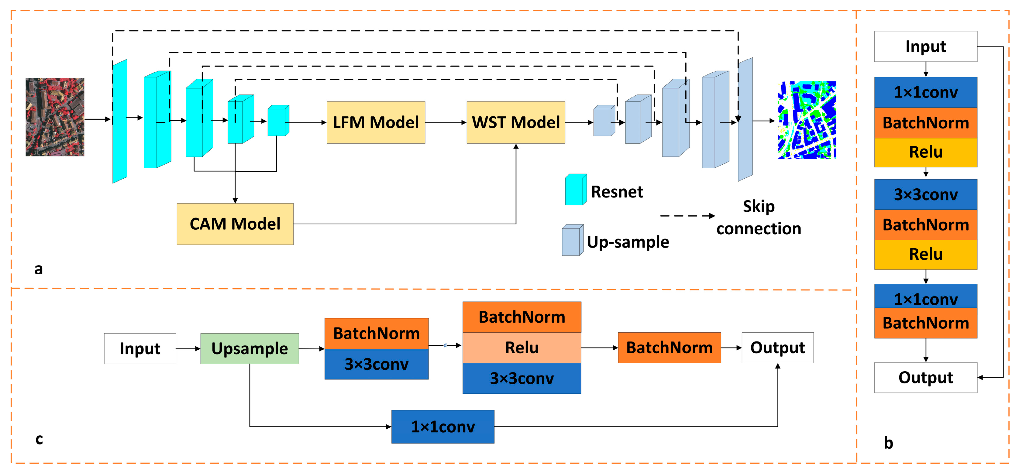
This section introduces the primary architecture of GLF-Net. As depicted in Figure 1a, an encoder–decoder architecture is employed. The encoder is comprised of a backbone network, alongside a global feature extraction module and a local feature extraction module. We use ResNet50 as the backbone network for feature extraction and down-sample; Figure 1b is a schematic of the ResNet50 residual block. Our CAM is applied to the final three layers of ResNet50, enabling the extraction of comprehensive global context features. The correlation between features is crucial for correctly distinguishing the semantic categories of features. By calculating the covariance matrix of features, we can understand the linear correlation between features, which helps us select the most discriminative combination of features. The extracted multi-scale contextual features can help GLF-Net obtain a wider range of contextual information, including the object’s global structure, background information, and contextual relationships, and also enable GLF-Net to better adapt to changes in different images and objects. This contextual information plays a pivotal role in achieving precise object segmentation, comprehending their semantics, and enhancing the overall generalization capability of GLF-Net. The regional fine-grained feature extraction module is used to extract local features, and the fine-grained module can refine the output of ResNet50. Fine-grained features can provide internal details of the object, which helps to distinguish different semantic categories and accurately classify internal regions. It can also capture small changes and edge details of the object to improve the accuracy of boundary recognition and segmentation. This gives better recognition results for small objects in the dataset.

In the decoder part, we built a WST module that employs the wavelet transform and self-attention to fuse the multi-scale features from the CAM and LFM modules. Then, a sequence of up-convolutions gradually expands the fused output to the original size. The wavelet transform has good sensitivity to edge and texture features. It helps to detect edge and texture information in an image and extract clear boundaries. In semantic segmentation, boundary information helps the model to obtain higher segmentation results. By applying the wavelet transform, the boundary information can be enhanced to improve the ability of GLF-Net to perceive object boundaries. The self-attention mechanism can model the global correlation of different positions in the input features instead of being limited to local regions. By calculating the attentional weights between each location in the input features, the self-attention mechanism can capture the long-range dependencies between different locations. This enables the self-attention mechanism to effectively model global contextual information in feature fusion. In the up-sampling process, as shown in Figure 1c, we designed the up-sampling part based on the ResNet residual block and use the jump connection strategy.

3.1. Global Feature Extraction

In convolutional neural networks, with the transformation of the sensory field and the gradual stacking of features, the semantic information contained in the deeper features of each layer is not exactly the same. Gradually, along with the change of the receptive field and characteristics of the stacked, each layer of ResNet deep features contained in the semantic information is not the same. In this regard, the fusion of multi-scale context information is crucial for the model. By this kind of information fusion, GLF-Net can adapt to different target dimensions effectively and handle the target boundary and complexity so as to improve the flexibility and generalization ability in semantic segmentation tasks.

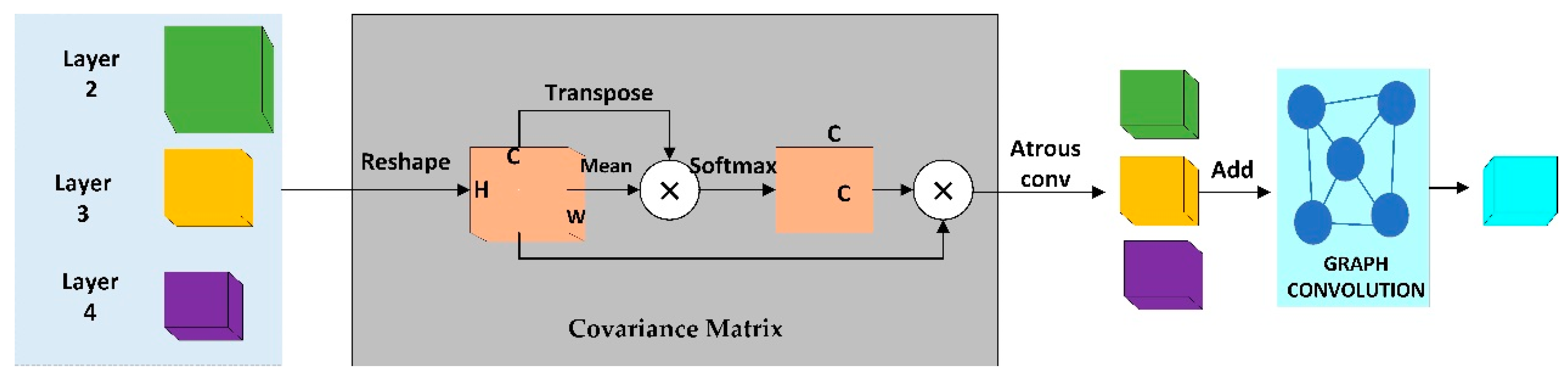
In the CAM module, we use a covariance matrix (CM) to model the relationship between channels [23], highlight the main channel information while providing a global summary, and then use graph convolution to encode the extracted features to capture the main context information in the last three layers of ResNet50. Figure 2 shows a visualization of the effect of the CM projection, with a1 and b1 showing the original image and a2 and b2 showing the effect of the image covariance projection matrix. It can be seen that the CM has a strong and prominent effect on the main information in the image. Based on this, as shown in Figure 3, we use the covariance matrix to extract the main information of the second-, third-, and fourth-layer features of ResNet50 in an attention mechanism. The first step is to perform the L2 normalization operation on the obtained features and then find the covariance matrix.

$$\mathit{cov}=\frac{1}{H\times W}{{\displaystyle \sum _{t=1}^{H\times W}\left(F^t-\overline{F^t}\right)}}^T\left(F^t-\overline{F^t}\right)$$

(1)

where $C$, $H$, and $W$ are the number of channels, height, and width; $t\in (1,2,\mathrm{\dots },H\times W)$; $F^t\in {ℝ}^{(H\times W)\times C}$; and $\overline{F^t}$ is the mean of $F^{{}^t}$. In the dot product process, subject to the effect of the broadcast mechanism, the covariance matrix $\mathit{cov}\in {ℝ}^{C\times C}$. Then, we obtain the corresponding covariance attention matrix by the $softmax$ function:

$$S(i)=\frac{\mathit{exp}(\mathit{cov}(i))}{{\displaystyle \sum _{i=1}^C\mathit{exp}(\mathit{cov}(i))}}$$

(2)

$$X(i)=F_m(i)\times S(i)$$

(3)

where $\mathit{cov}(i)$ represents the middle element of the covariance matrix. The result, $X(i)$, of the covariate attention is obtained by multiplying the original feature, F, with the covariate attention matrix, S. Then, we use covariance attention to extract the main information in this layer. In order to effectively fuse the features of the three layers, we use the dilated convolution strategy to down-sample the features of the second and third layers so that the three-layer features obtain feature maps of the same size. The expanded convolution enables GLF-Net to obtain a larger receptive field, thereby obtaining wider context information. Finally, the three layers of features are added to obtain the fusion feature.

After obtaining the fused multi-scale context features, we use graph convolution [33] to model the global context information of the features. First, our approach involves the projection of the input feature map from the coordinate space onto a graph composed of latent nodes or regions within the interaction space. These latent nodes adeptly aggregate local descriptors using convolutional layers, strategically diminishing the impact of superfluous attributes within the coordinate space. Subsequently, the interrelationships among these nodes are comprehensively deduced through a duo of one-dimensional convolutions.

$$Z=GX{w}_g$$

(4)

where G denotes the adjacency matrix that propagates information across nodes and the adjacency matrix learns edge weights reflecting the relationship between the underlying global pooled features at each node. $w_g$ represents the graph convolution parameters. G and $w_g$ are learned autonomously with gradient descent as the model is continuously trained. During training, the graph’s affinity matrix learns the edge weights, thus capturing the nuanced connections between nodes within a fully interconnected graph. This design ensures that each node assimilates information from all the other nodes, constantly updating its state. Upon inference, the output features undergo a transformation back into the original space, yielding the derivation of our global features.

3.2. Local Fine-Grained Feature Extraction

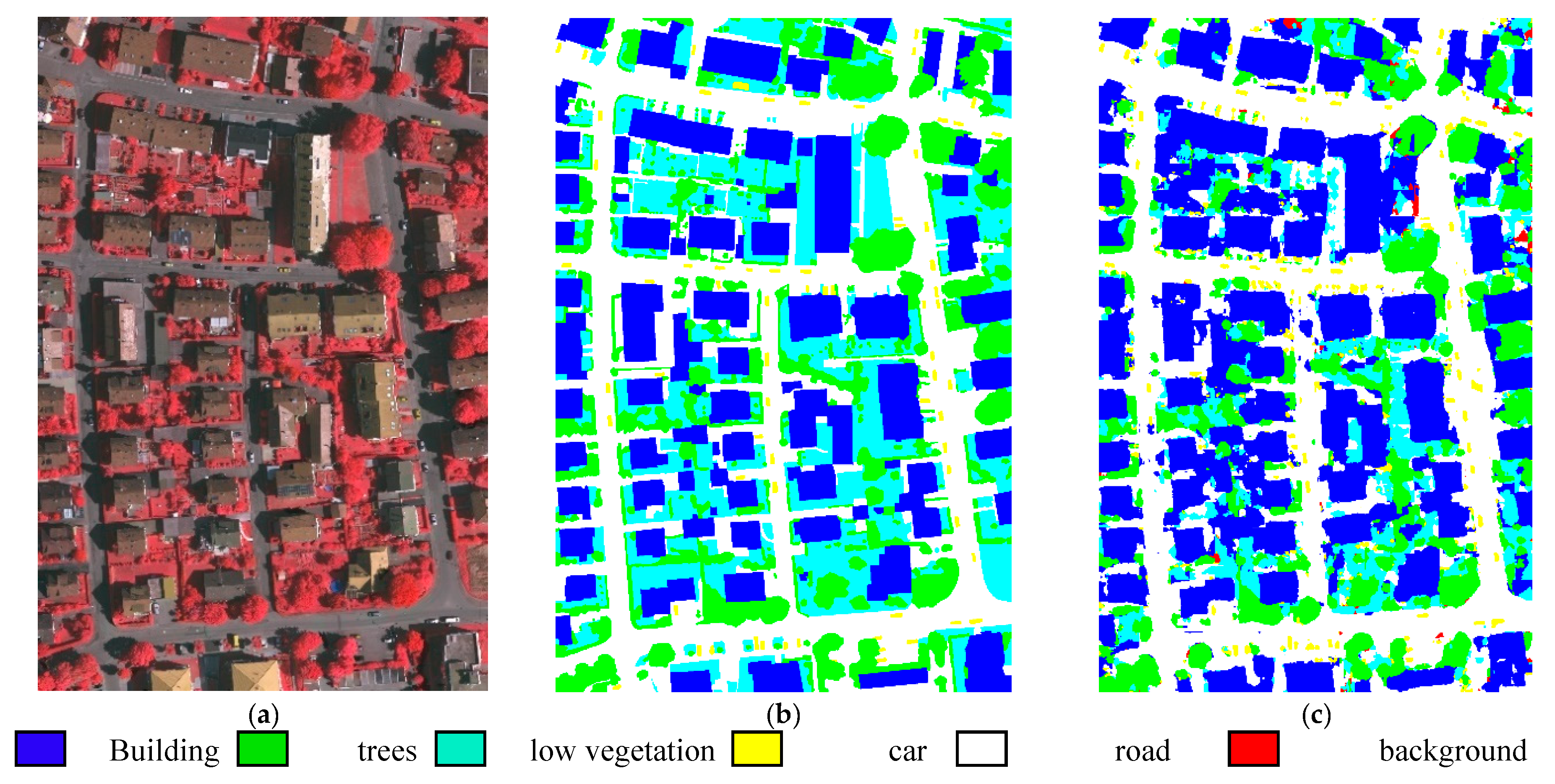
HR remote sensing images have the characteristics of high within-class variance and low within-class variance. In HR remote sensing images, as shown in Figure 4, some small objects present in complex environments are usually misclassified. Therefore, diverging from global features, local features place greater emphasis on recognizing and classifying intricate fine-grained attributes within images. After down-sampling by ResNet, the model eventually extracts a feature map of dimensions 8 × 8; each feature value represents a region of the original image [34]. Through the inference screening of this module, the features of small objects are obtained and highlighted by up-sampling.

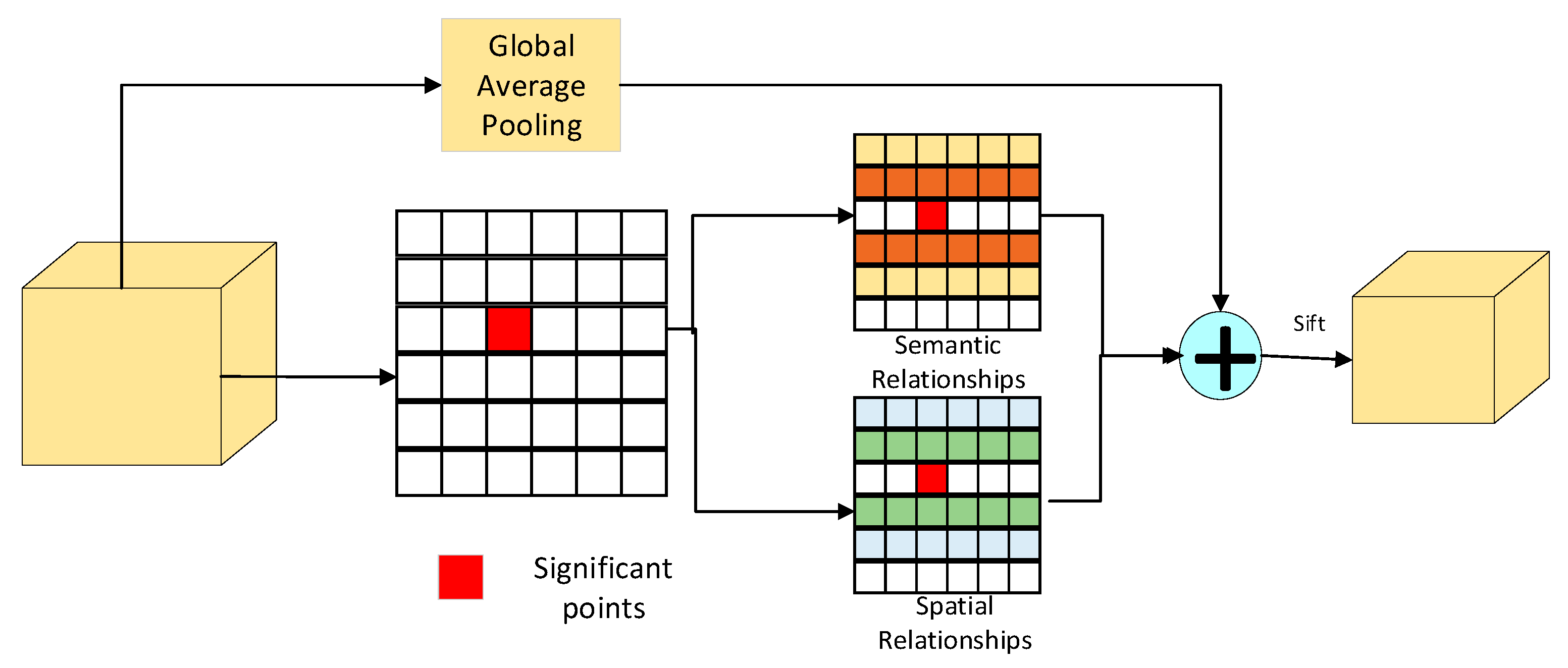
Our local feature extraction module is shown in Figure 5. First, we evenly divide our feature map, $V$$\in R^{(H\times W)}$, into t local areas.

$$V_{hw}={\displaystyle {\sum }_{t=1}^D{F}_{thw}}$$

(5)

where $V_{hw}$ represents the information in the dimension $(h,w)$ of V and $F_{thw}$ represents the information in the dimension $(t,h,w)$ of F. We obtain fine-grained local features through semantic and spatial relationships between feature points in each local area. The individual feature points in our local region, $V_{hw}$, are set to $P_j$. Specifically, we take the peak point within each local region as the salient point, $P_n$, and use it as a benchmark to compute semantic and spatial relationships with each point within the local region.

As mentioned above, the context relationship is particularly important in the task of semantic segmentation, and the simple region division can easily cause the loss of context information in the feature map. To this end, we first calculate the spatial relationship between salient points, $P_n$, and each feature point, $P_j$, in each local area based on Euclidean distance, as $C{R}_{nj}$:

$$C{R}_{nj}=\sqrt{{({\mathit{P}}_n(x)-{\mathit{P}}_j(x))}^2+{({\mathit{P}}_n(y)-{\mathit{P}}_j(y))}^2}$$

(6)

where $j=1,\cdot \cdot \cdot ,H\times W$.The smaller the value of $C{R}_{nj}$, $P_n$ and $P_j$ get closer. We then use the cosine similarity to calculate the semantic dependency between the salient point, $P_n$, and the rest of the feature points, $P_j$:

$$S{R}_{nj}=\frac{Q_n{}^{{}^T}{Q}_j}{\left|\right|Q_n\left|\right|\left|\right|Q_j\left|\right|}$$

(7)

where $Q_n$∈ $R^D$ and $Q_j$∈ $R^D$ are the channel features of point $P_n$ and point $P_j$ in each local area. Considering both spatial relationship and semantic similarity, we define the spatial semantic relationship, $R_{nj}$, as follows:

$$R_{nj}=\frac{S{R}_{nj}}{{\mathit{CR}}_{nj}+1}$$

(8)

The correlation between point $P_n$ and point $P_j$ is proportional to the value of R. Then, we can obtain the local features, $F_n^l$, of salient points, $P_n$, by aggregating spatial semantic context information, which is formulated as follows:

$$F_n^l={\displaystyle {\sum }_{j=1}^{H*W}\frac{exp(R_{nj})}{{\displaystyle {\sum }_{j=1}^{H*W}exp(R_{nj})}}}$$

(9)

After obtaining all the local features, to filter the features of the small target we need from these local features, we first obtain the global features of the original feature, which is denoted as $F^{\mathrm{G}}$:

$$F^{\mathrm{G}}=\mathrm{GAP}\left(\mathrm{F}\right)$$

(10)

where $\mathrm{GAP}$ is the global average pooling. The semantic similarity between each local feature and the global pooling result is then calculated using the cosine similarity and by screening the k groups of local features that are most dissimilar to the global feature, which are the local small target features we need to extract.

3.3. Fusion Module

In CNNs, both convolution and pooling operations inherently entail a certain degree of information loss across different frequencies. However, by incorporating the wavelet transform, the model enables the fusion of various frequency characteristics and the preservation of multi-scale information fusion. This approach optimally exploits the complementarity between high- and low-frequency data.

The deeper convolutional neural network architectures show greater ability to improve the segmentation accuracy of complex image edge contours and details while retaining the multi-frequency attributes. Wavelet transform, employing an array of diverse scale wavelets, decomposes the original function. This process yields coefficients representing the original function under distinct scale wavelets through translation and scale transformations. The translation affords insight into the temporal attributes of the original function, while scale transformation elucidates its frequency characteristics.

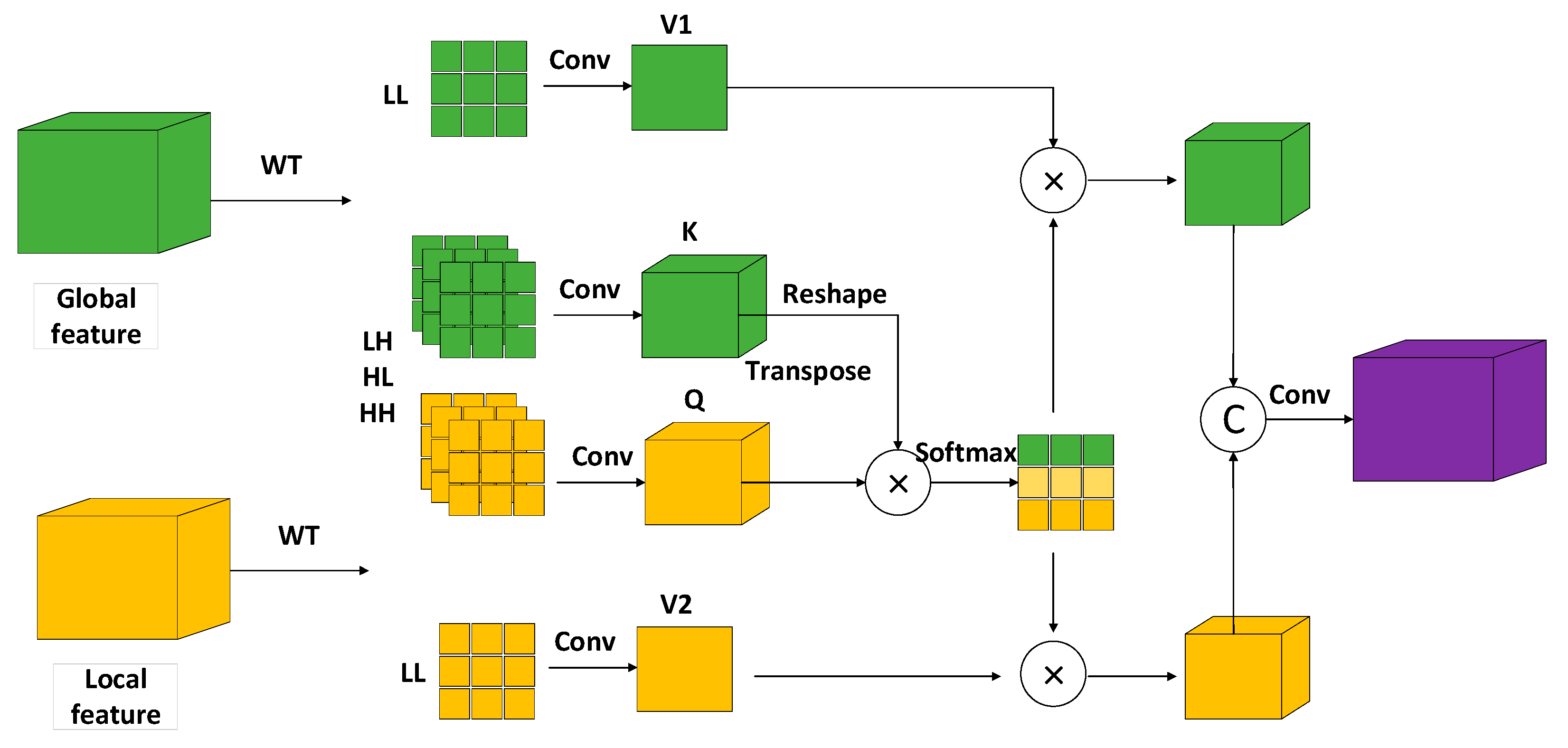
Having extracted the global and local features, the subsequent phase revolves around their effective fusion. As depicted in Figure 6, our fusion module harnesses a combination of wavelet transform and self-attention mechanisms to accomplish this fusion task:

We first use the 2D Haar transform on the global and local features to obtain the low-frequency component, $x_{LL}$, and three high-frequency components, $x_{LH}$,$x_{HL}$, and $x_{HH}$. The four frequency band components are obtained by Equation (11):

$$\begin{array}{l}{\mathit{x}}_{LL}(i,j)=\mathit{x}(2i-1,2j-1)+\mathit{x}(2i-1,2j)+\mathit{x}(2i,2j-1)+\mathit{x}(2i,2j)\\ {\mathit{x}}_{LH}(i,j)=-\mathit{x}(2i-1,2j-1)-\mathit{x}(2i-1,2j)+\mathit{x}(2i,2j-1)+\mathit{x}(2i,2j)\\ {\mathit{x}}_{HL}(i,j)=-\mathit{x}(2i-1,2j-1)+\mathit{x}(2i-1,2j)-\mathit{x}(2i,2j-1)+\mathit{x}(2i,2j)\\ {\mathit{x}}_{HH}(i,j)=\mathit{x}(2i-1,2j-1)-\mathit{x}(2i-1,2j)-\mathit{x}(2i,2j-1)+\mathit{x}(2i,2j)\end{array}$$

(11)

where $i=1,2,\mathrm{\dots },H/2,j=1,2,\mathrm{\dots },W/2$ and $H$ and $W$ are the height and width of the original feature map, respectively. That is, the width and height of the output component of each level of the DWT will be $1/2$ that of the input image.

V1 and V2 of the self-attention module are obtained by performing a convolution operation on the low-frequency components of the two features. Subsequently, the high-frequency components undergo convolution to yield the $Q$ and $K$ elements of the self-attention module, where $Q, K\in R^{c_k\times H_l\times W_l}$ and $C_K$ is the number of channels in the low-dimensional mapping space. Then, we reshape them into the shape of $C_K\times N$, where $N=H_l\times W_l$ is the number of pixels. Diverging from traditional self-attention mechanisms, our $Q$ and $K$ features establish a mutual interplay to facilitate cross-image information exchange. In light of this, we introduce the concept of two distinct branches tailored to amplify the representation of support and query features. Following this, a matrix multiplication is executed, utilizing the transposed forms of $Q$ and $K$. This operation culminates in the creation of a novel feature map, which is subsequently transposed once more to derive the feature map for the alternate branch. Lastly, a $softmax$ module is applied to each of these derived maps, individually generating spatial attention maps for the $Q$ and $K$ branches, thereby completing this process [35].

$$A_{ji}=\frac{exp(Q_i\times K_j)}{{\displaystyle {\sum }_{i=1}^{N}exp(Q_i\times K_j)}}$$

(12)

where $A_{ji}$ measures the impact of querying the ith position on supporting the jth position. The enhanced similarity in feature representations between two locations corresponds to a heightened correlation between them. Then, the final fused features, $A_{ji}$, are obtained by concatenating them with V1 and V2, respectively.

4. Experimental Results and Analysis

4.1. Data Sets

We validated the performance of GLF-Net using two state-of-the-art airborne image datasets from the City Classification and 3D Building Reconstruction Test projects provided by ISPRS, which are available from the URL Semantic Annotation Benchmark (https://www.isprs.org/education/benchmarks/UrbanSemLab/Default.aspx, accessed on 26 May 2022). The dataset utilizes a Digital Terrain Model (DSM) produced through HR orthogonal photographs and complementary dense image-matching methodologies. Both datasets encompass urban landscapes, capturing diverse urban scenes. Vaihingen portrays a quaint village characterized by numerous individual buildings and multi-story edifices. On the other hand, Potsdam stands as a quintessential historical city replete with expansive building complexes, narrow alleyways, and densely clustered settlement formations. In a meticulous effort, each dataset has been subject to manual classification, resulting in the categorization of land cover into the six most prevalent classes.

(1) Vaihingen dataset: Comprising 33 distinct remote sensing images of varying dimensions, each image is meticulously extracted from a larger-scale orthophoto picture at the top level. A careful image selection process ensures the avoidance of data gaps. The remote sensing images adhere to an 8-bit TIFF file format, encompassing three bands: near-infrared, red, and green. Meanwhile, the DSM is represented as a single-band TIFF file, with its grayscale values (indicative of DSM height) encoded in 32-bit floating point format. The HR remote sensing images and the DSM both share a ground sampling distance of 9 cm. The DSM data are ingeniously derived through dense image matching utilizing the Trimble INPHO 5.3 software. Presented in various channel combinations, HR remote sensing images adopt the form of TIF files, with each channel sporting an 8-bit spectral resolution. Both the HR remote sensing images and label maps take on the form of three-channel images, while DSM data maps are presented as single-channel images. The HR remote sensing images are stored as 8-bit TIF files, each equipped with three frequency bands. These RGB bands correspond to the near-infrared, red, and green bands captured by the camera. Notably, a DSM is encapsulated within a TIFF file, featuring a single frequency band, and its gray levels are encoded as 32-bit floating point values. It is worth mentioning that HR remote sensing images are spatially defined within the same grid as the DSM, thereby eliminating the necessity to factor in geocoding information during processing.

(2) Potsdam Dataset: Comprising 28 images, all uniformly sized, the spatial resolution of the top image is an impressive 5 cm. Parallel to the Vaihingen dataset, this collection is constructed from remote sensing TIF files characterized by three bands, alongside DSM data, which remain as a single band. It is noteworthy that each remote sensing image within this dataset boasts identical area coverage dimensions.

4.2. Parameter Setting and Evaluation Index

We trained our model within the PyTorch framework, conducting experiments on HR remote sensing image datasets. These experiments were executed on a personal computer featuring an 11th-generation Intel(R) Core(TM) i9-11900F CPU clocked at 2.50GHz(Intel Productions), an NVIDIA GeForce RTX 3090 GPU, and 32 GB of memory (Asus Productions). An initial learning rate of 0.0001 was adopted, spanning a comprehensive training regimen of thirty epochs. The learning rate underwent adjustments every ten epochs, facilitating progressive optimization. For loss computation, the cross-entropy loss function was employed, aiding in the convergence of training. To accommodate the input data within GLF-Net, we meticulously partitioned the HR remote sensing image into smaller 256x256 patches. We introduced image flipping and rotation. These data augmentation techniques effectively expanded the dataset and enhanced its diversity.

The evaluation of GLF-Net’s performance was accomplished using metrics such as mean intersection over union (IoU), intersection over union (IoU), overall accuracy, and mean F1-score. $\mathrm{IoU}$ is the proportion of the intersection to the union between the predicted outcome and the ground truth value and is calculated for use case segmentation. $\mathrm{mIoU}$ is a standard assessment, and it is the mean of all categories of $\mathrm{IoU}$. $\mathrm{F}1$ is a weighted average of the precision and recall of GLF-Net. From the confusion matrix, we can calculate $\mathrm{mIoU}$, $\mathrm{IoU}$, $\mathrm{OA}$, and $\mathrm{F}1$:

$$\mathrm{O}\mathrm{A}=\frac{{\displaystyle {\sum }_{K=1}^{K}T{P}_K}}{{\displaystyle {\sum }_{K=1}^{K}T{P}_K+F{P}_K+T{N}_K+F{N}_K}}$$

(13)

$$\mathrm{IoU} =\frac{{\displaystyle {\sum }_{K=1}^{K}T{P}_K}}{{\displaystyle {\sum }_{K=1}^{K}T{P}_K+F{P}_K+F{N}_K}}$$

(14)

$$\mathrm{mIoU} =\frac{1}{K}\frac{{\displaystyle {\sum }_{K=1}^{K}T{P}_K}}{{\displaystyle {\sum }_{K=1}^{K}T{P}_K+F{P}_K+F{N}_K}}$$

(15)

$$\mathrm{mF}1 =\frac{1}{K} {\displaystyle {\sum }_{K=1}^{K}2\times \frac{precisio{n}_K\times recal{l}_K}{precisio{n}_K+recal{l}_K}}$$

(16)

where TP and TN represent the number of correct and incorrect positive samples, respectively; FP and FN represent the number of negative samples that were correctly and incorrectly judged, respectively; and $precisio{n}_K=$$T{P}_{\mathrm{K}}/(T{P}_{\mathrm{K}}+F{P}_{\mathrm{K}})$ and $recal{l}_K=$$T{P}_{\mathrm{K}}/(T{P}_{\mathrm{K}}+F{N}_{\mathrm{K}})$ are the precision and recall of GLF-Net, respectively.

4.3. Semantic Results and Analysis

This section primarily presents the outcomes attained by GLF-Net. As depicted in Figure 7, the confusion matrix provides a comprehensive overview of our model’s performance across these two datasets. Figure 8 and Figure 9 showcase the segmentation results of HR remote sensing images: Figure 8 corresponds to the Potsdam dataset, and Figure 9 pertains to the Vaihingen dataset. Figure 8 and Figure 9 have the same legend. Notably, GLF-Net demonstrates commendable performance on both datasets, substantiating its efficacy in semantic segmentation tasks.

To further verify the performance of GLF-Net, we set up a quantitative comparison experiment. We compared GLF-Net with four models: Unet, deeplabV3+, $A^2$-FPN, and BSE-Net [36], and each model consistently uses ResNet50 as the baseline network. DeeplabV3+ employs dilated convolutions to acquire features spanning multiple scales, thereby facilitating the extraction of contextual information. $A^2$-FPN also aggregates global features for image semantic segmentation and derives discriminative features through the accumulation and dissemination of multi-level global contextual attributes. The Bes-Net model is based on boundary information, and incorporating multi-scale context information enhances the precision of the semantic segmentation model.

Table 1. Comparative experiments on the Vaihingen dataset.

Model	IoU					mIoU	F1	OA
	Building	Low-Veg	Surface	Tree	Car
Unet	0.795	0.866	0.632	0.744	0.504	0.682	0.804	0.863
DeeplabV3+	0.755	0.826	0.622	0.737	0.513	0.658	0.784	0.846
$A^2$-FPN	0.817	0.887	0.667	0.771	0.622	0.748	0.853	0.881
Bes-Net	0.830	0.899	0.698	0.789	0.658	0.774	0.871	0.892
OURS	0.833	0.902	0.692	0.781	0.668	0.780	0.869	0.894

and

Table 2. Comparison experiments on the Potsdam dataset.

Model	IoU					mIoU	F1	OA
	Building	Low-Veg	Surface	Tree	Car
Unet	0.814	0.878	0.704	0.774	0.473	0.715	0.827	0.881
DeeplabV3+	0.840	0.924	0.741	0.725	0.777	0.758	0.857	0.890
$A^2$-FPN	0.869	0.943	0.782	0.759	0.808	0.800	0.886	0.911
Bes-Net	0.871	0.944	0.786	0.770	0.825	0.803	0.887	0.913
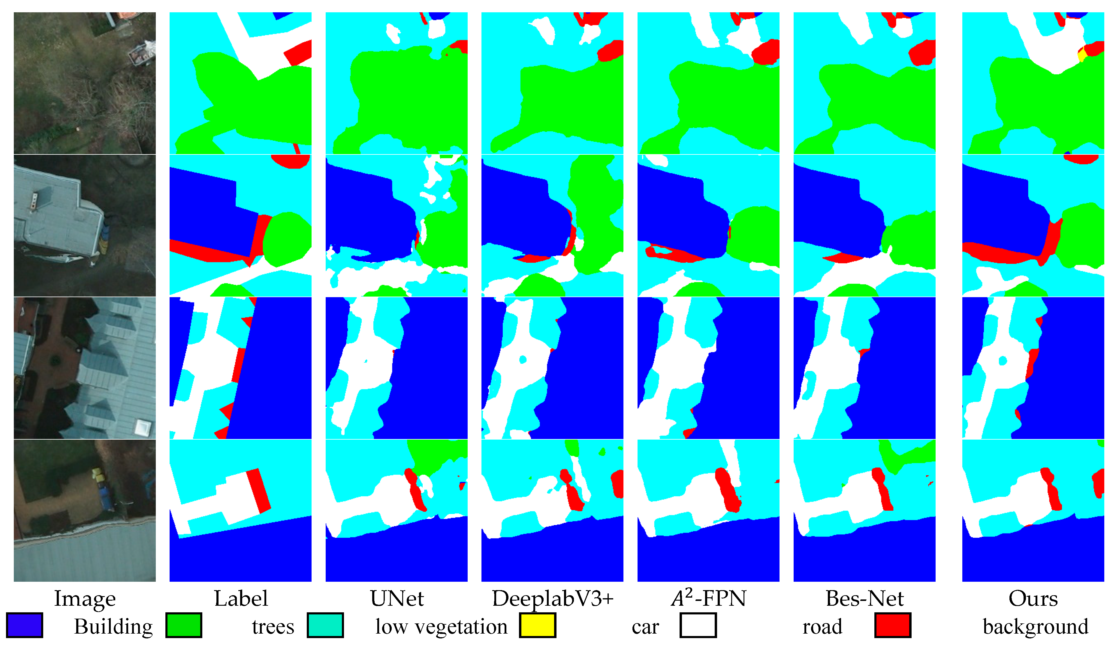
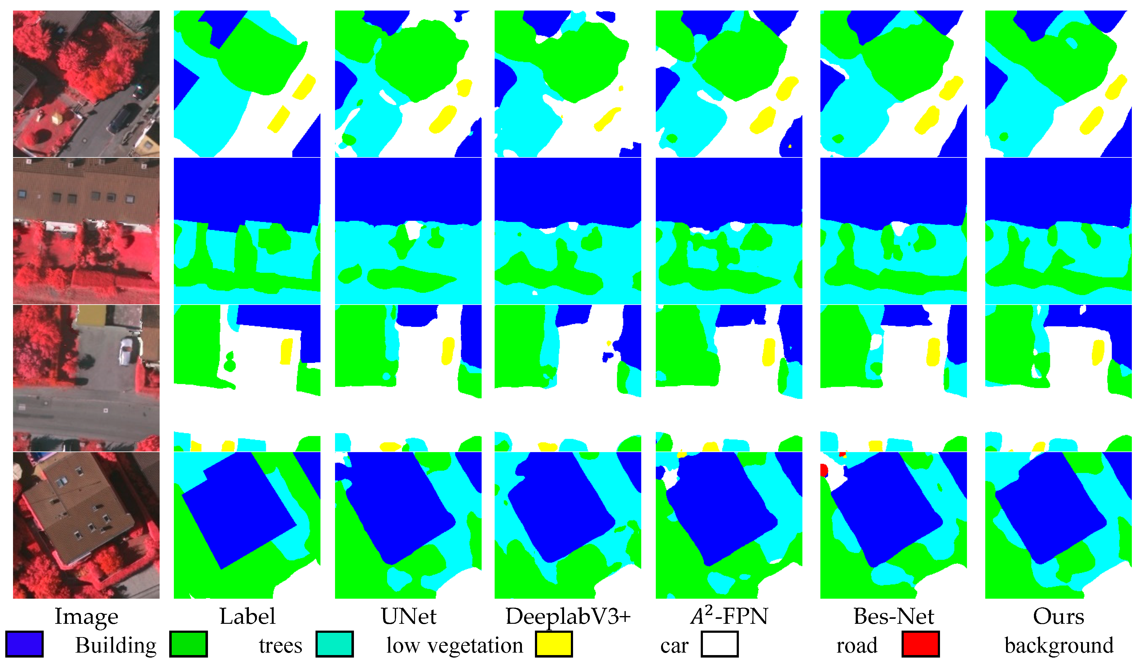
OURS	0.876	0.946	0.791	0.770	0.827	0.811	0.893	0.916

present the comparative results from the experimentation conducted on the Vaihingen and Potsdam datasets, respectively. We bold the optimal metrics. Additionally, select outcomes from the test set are showcased in Figure 10 and Figure 11. Notably, GLF-Net demonstrated superior performance across these evaluations. In particular, it stands out for its reduced incidence of misclassified segments and its improved proficiency in discerning certain boundaries and smaller objects. For instance, in the Potsdam dataset, GLF-Net excels at distinguishing the delineation between road and low vegetation. Moreover, the Vaihingen dataset showcases a heightened aptitude for identifying diminutive elements, like trees and cars.

4.4. Ablation Experiments

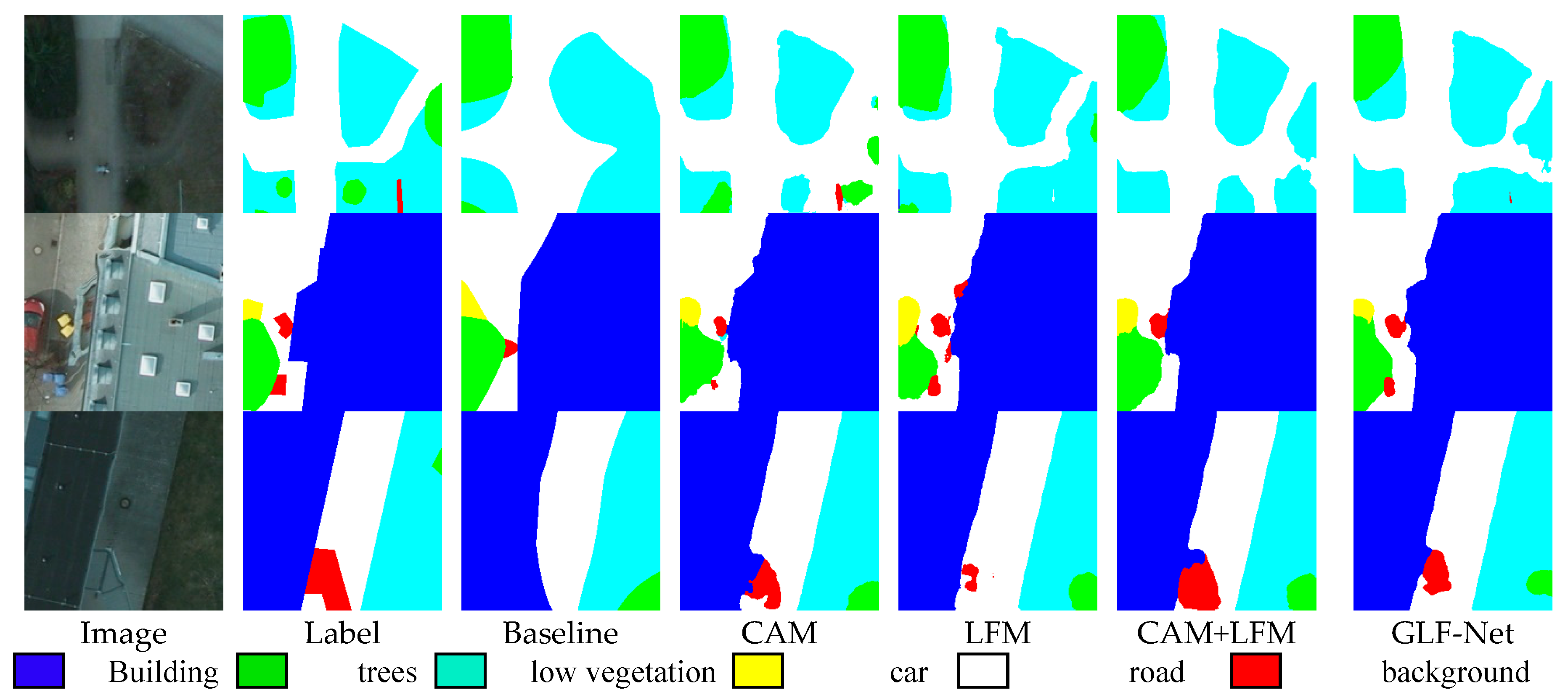
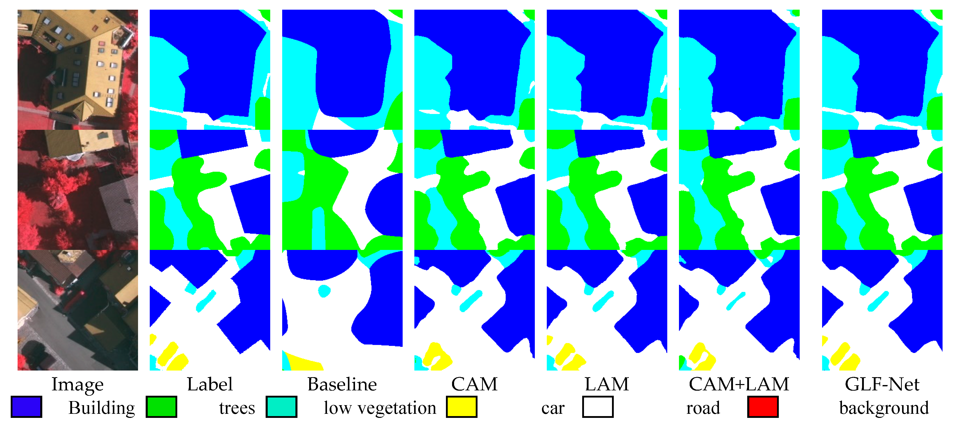
GLF-Net makes full use of the global context information extracted by CAM, LFM extracts fine-grained local features to make GLF-Net better improve the recognition and classification of small targets, and WST effectively integrates the two. To verify that each module can fully play its role, we set up two sets of ablation experiments to verify the performance of our module. Firstly, the ablation strategies of the first group are the baseline network, adding CAM, adding LFM, adding CAM and LFM, and adding three modules (GLF-Net) to verify the performance of our three modules.

Table 3. Ablation experiments on the Vaihingen dataset.

Model	IoU					mIoU	F1	OA
	Building	Low-Veg	Surface	Tree	Car
Baseline	0.715	0.823	0.584	0.678	0.531	0.592	0.714	0.821
CAM	0.829	0.898	0.687	0.777	0.659	0.764	0.864	0.887
LFM	0.826	0.899	0.685	0.774	0.660	0.761	0.862	0.886
CAM+LFM	0.828	0.900	0.685	0.774	0.652	0.766	0.865	0.888
OURS	0.833	0.902	0.692	0.781	0.668	0.780	0.869	0.894

showcases the outcomes of ablation experiments conducted on the Vaihingen dataset, while

Table 4. Ablation experiments on the Potsdam dataset.

Model	IoU					mIoU	F1	OA
	Building	Low-Veg	Surface	Tree	Car
Baseline	0.788	0.922	0.720	0.728	0.569	0.680	0.795	0.873
CAM	0.869	0.938	0.774	0.769	0.818	0.803	0.887	0.912
LFM	0.865	0.941	0.776	0.763	0.824	0.793	0.880	0.908
CAM+LFM	0.872	0.945	0.787	0.765	0.827	0.806	0.889	0.913
OURS	0.876	0.946	0.791	0.770	0.827	0.811	0.893	0.916

presents the results of ablation experiments performed on the Potsdam dataset. We bold the optimal metrics. Moreover, Figure 12 and Figure 13 visually illustrate the findings from ablation experiments on the Vaihingen and Potsdam datasets, respectively. A detailed analysis of the data in these two tables indicates that our modules significantly elevated the performance of GLF-Net when contrasted with the baseline network. And it can be seen from the results that the addition of three modules at the same time is superior to the baseline module and the single use of modules in terms of overall classification and the identification of boundaries and small targets.

To verify which stage of context information of ResNet is most needed for GLF-Net, we set up a second set of ablation experiments to compare the performance of CAM. Our CAM module is used for ResNet stages 123, 124, 134, and 234. Finally,

Table 5. CAM ablation experiment on the Vaihingen dataset.

Model	IoU					mIoU	F1	OA
	Building	Low-Veg	Surface	Tree	Car
CAM123	0.827	0.891	0.685	0.779	0.647	0.762 ± 0.01	0.862	0.886
CAM124	0.827	0.887	0.685	0.779	0.650	0.761 ± 0.01	0.862	0.886
CAM134	0.827	0.887	0.685	0.779	0.650	0.761 ± 0.01	0.862	0.886
CAM_nonCM	0.820	0.895	0.675	0.775	0.631	0.755 ± 0.02	0.857 ± 0.01	0.885 ± 0.01
CAM_nonGrapth	0.821	0.893	0.677	0.775	0.608	0.749 ± 0.02	0.853 ± 0.01	0.885 ± 0.01
DANet	0.826	0.885	0.686	0.776	0.643	0.761 ± 0.03	0.862 ± 0.01	0.886 ± 0.01
CAM234	0.829	0.898	0.687	0.777	0.659	0.764 ± 0.03	0.864 ± 0.01	0.887 ± 0.01

and

Table 6. CAM ablation experiment on the Potsdam dataset.

Model	IoU					mIoU	F1	OA
	Building	Low-Veg	Surface	Tree	Car
CAM123	0.870	0.943	0.783	0.768	0.818	0.801 ± 0.01	0.886	0.911
CAM124	0.869	0.938	0.784	0.767	0.819	0.800 ± 0.01	0.885	0.911
CAM134	0.869	0.938	0.784	0.767	0.819	0.800 ± 0.02	0.885	0.911
CAM_nonCM	0.868	0.935	0.776	0.754	0.815	0.798 ± 0.02	0.882 ± 0.02	0.909 ± 0.01
CAM_nonGrapth	0.868	0.936	0.779	0.762	0.812	0.798 ± 0.02	0.883 ± 0.02	0.909 ± 0.01
DANet	0.867	0.935	0.776	0.757	0.810	0.797 ± 0.03	0.882 ± 0.02	0.909 ± 0.01
CAM234	0.869	0.944	0.777	0.769	0.822	0.803 ± 0.02	0.887 ± 0.01	0.912 ± 0.01

present the experimental results derived from the Vaihingen dataset and the Potsdam dataset, respectively. The outcomes distinctly highlight the superiority of the CAM module, showcasing its optimal performance when applied to the 234 stages. At the same time, in order to verify the effect of the covariance matrix and graph convolution, we also performed a comparison with two models without using the covariance matrix and without using graph convolution. As shown in Figure 5 and Figure 6, there is a large gap between the performance of the two and CAM. We bold the optimal metrics. Finally, in order to verify the superiority of the CAM module, we also made a comparison with the existing model DANet. The CAM module shows better performance than DANet on both datasets.

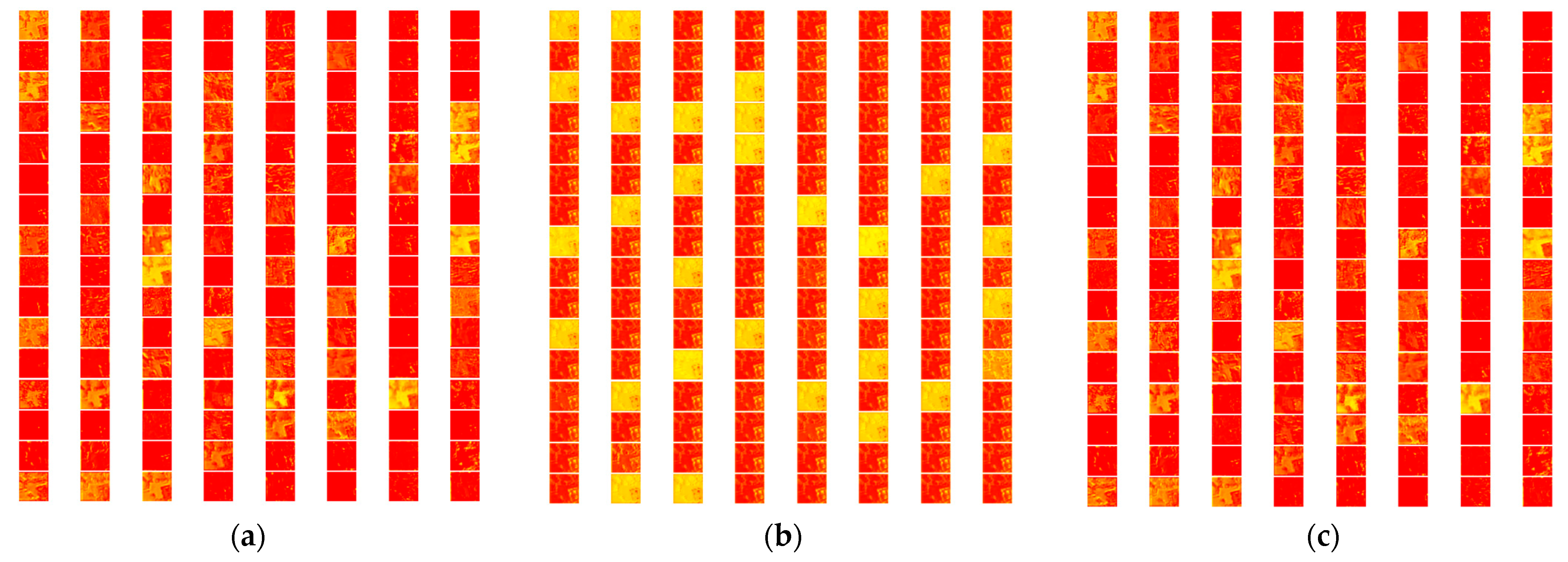
In particular, to visualize the role of the CAM module in extracting and enhancing contextual features, we visualized ResNet, the CAM module, and the intermediate features of DANet, as shown in Figure 14. The red channel represents a higher degree of responsiveness, while the opposite is true for yellow. Compared to ResNet, DANet does not show significant changes, while CAM extracts channels with primary information.

Finally, in order to verify the performance of the self-attention module in our WST module, we performed ablation experiments on the WST module.

Table 7. WST ablation experiment on the Potsdam dataset.

Model	IoU					mIoU	F1	OA
	Building	Low-Veg	Surface	Tree	Car
Non_self attention	0.870	0.945	0.779	0.758	0.820	0.806	0.890	0.912
GLF-Net	0.876	0.946	0.791	0.770	0.827	0.811	0.893	0.916

and

Table 8. WST ablation experiment on the Vaihingen dataset.

Model	IoU					mIoU	F1	OA
	Building	Low-Veg	Surface	Tree	Car
Non_self attention	0.821	0.891	0.677	0.774	0.610	0.750	0.854	0.844
GLF-Net	0.833	0.902	0.692	0.781	0.668	0.780	0.869	0.894

give the results of the ablation experiments. We bold the optimal metrics. It can be seen from the results that the self-attention module has brought significant improvements.

5. Conclusions

This paper introduces the GLF-Net model for semantic segmentation of HR remote sensing images. This model addresses the complex challenges posed by significant intra-class differences and small inter-class differences in HR remote sensing images. The proposed GLF-Net employs an encoder–decoder architecture with ResNet50 as the base network. The model uses the CAM module to extract global contextual features, uses the LFM module to extract complex local features, and uses WST to effectively integrate these two features. Through the above modules, the proposed GLF-Net simultaneously obtains broader global context information and fine-grained local texture and boundary features, which significantly enhances the model’s ability to recognize smaller objects and contributes to the overall enhancement of segmentation performance. The validation of our model on ISPRS’s Vaihingen and Potsdam datasets confirms its superior achievement, with GLF-Net outperforming other models when all three modules are effectively integrated.

Although the proposed GLF-Net has achieved good results, it still has a high computational cost, and, next, we will research reducing the complexity of the model while maintaining the existing performance.