Analysis of Mass Wasting Processes in the Slumgullion Landslide Using Multi-Track Time-Series UAVSAR Images

Abstract

The Slumgullion landslide is a large translational debris slide whose currently active part has likely been sliding for approximately 300 years. Its permanent motion and evolutionary processes have attracted the attention of many researchers. In order to study its mass wasting processes and evolution trend, the spatial–temporal displacement of the Slumgullion landslide was retrieved using an adaptive pixel offset tracking (POT) method with multi-track Uninhabited Aerial Vehicle Synthetic Aperture Radar (UAVSAR) images. Based on three-dimensional displacement and slope information, we then revealed the spatial–temporal distribution of surface mass depletion or accumulation in the landslide, which provides a new perspective to analyze the evolutionary processes of landslides. The results indicate that the Slumgullion landslide had a spatially variable displacement, with a maximum displacement of 35 m. The novel findings of this study mainly include two parts. First, we found that the surface mass accumulated in the toe of the landslide and depleted in the top and middle area during the interval, which could increase the resisting force and decrease the driving force of the Slumgullion landslide. This result is compelling evidence which indicates the Slumgullion landslide should eventually tend to be stable. Second, we found that the distribution of geological structures can well explain some of the unique mass wasting in the Slumgullion landslide. The larger local mass depletion in the landslide neck area verifies that the sharp velocity increase in this region is not only caused by the reduction in width but is also significantly affected by the local normal faults. In summary, this study provides an insight into the relation between the landslide motion, mass volume change, and geological structure. The results demonstrate the great potential of multi-track airborne SAR for displacement monitoring and evolutionary analysis of landslides.

1. Introduction

Landslides, as a type of geological hazard, are a common occurrence and usually cause large economic and human losses [1,2,3,4]. They are accompanied by a series of measurable changes in physical information during its evolution, for example, landslide displacements and mass depletion or accumulation. This physical information is closely related to the internal structure and stress of landslides [5]. Analysis of mass wasting processes based on surface spatial–temporal displacements can help to better understand the kinematic characteristics of landslides and the mechanisms of evolution, which is also fundamental to managing landslide risks [6,7,8].

In order to investigate and monitor landslide, many techniques and tools have been tried. Field surveys were the primary method of landslide investigation in the early days. They can provide detailed data for a landslide study based on various close observation tools, such as the Global Position System (GPS) [9,10], clinometers [11], and water level gauge [12]. These in situ monitoring techniques based on point measurements only provide information concerning their surroundings and are generally not suitable for landslide monitoring in inaccessible or wide areas. Remote sensing has excellent potential for landslide investigation due to its wide spatial coverage and high efficiency, and has been widely used in recent years. Optical remote sensing images can identify a set of morphological features (e.g., shape, size, spectral, texture, and pattern) associated with landslides and image correlation can be used to monitor landslide motion [13,14]. However, daylight and weather conditions (i.e., clouds) still hamper the acquisition of suitable images. LiDAR is another crucial remote sensing tool for landslide investigation, which can penetrate vegetation to retrieve elevation information on the bare ground [15]. The displacement field of landslides can be monitored via multi-temporal LiDAR surveys, although at a relatively high cost.

With the ability of all-day and all-climate observation, synthetic aperture radar (SAR) technology is an advanced tool widely applied for landslide monitoring [16,17,18]. Compared with point-based observations, SAR has the potential to provide landslide-wide observations with high spatial resolution, which contribute to understanding the landslide internal mechanisms. There are three main methods to measure landslide displacement using SAR images: (1) Differential interferometric SAR (D-InSAR) [19] and time-series InSAR (e.g., PS-InSAR and SBAS-InSAR) [20,21]; this kind of method can obtain subtle displacement along the line-of-sight (LOS) direction with high precision but is limited by phase decoherence or maximum detectable gradients. (2) Multiple-aperture SAR interferometry (MAI) [22]; it can measure surface displacement in the azimuth direction by means of split-beam SAR processing but is sensitive to phase noise due to temporal–spatial decorrelation. (3) Pixel offset tracking (POT) [23], which can measure large-gradient displacement along both the azimuth and range directions. Compared to InSAR and MAI, POT can tolerate much larger displacement gradients but with a relatively low measurement precision depending on the SAR image resolution [24]. Recently, the resolution of SAR images has been improved to sub-meter level, which has greatly facilitated the application of the POT method.

Although, InSAR, MAI, and POT with single track can extract the one- or two-dimensional (i.e., azimuth and range directions) displacement of landslides, which still limits the analysis and interpretation for landslide motion in geographical space. The integration of ascending and descending measurements with multiple methods (i.e., InSAR, MAI, and POT) is a common method for three-dimensional (3D) displacement estimation with spaceborne SAR [25,26]. Compared to Spaceborne SAR, airborne SAR is more agile and convenient to enable the acquisition of multi-aspect/multi-angular obversions in the same area, which is necessary for 3D displacement estimation with SAR images. In view of the advantages and applicability, POT with airborne SAR images is applicable for large-gradient landslide 3D displacement mapping.

The Slumgullion landslide, as a large translational debris slide, is located in southwestern Colorado, United States [27]. The most peculiar fact is its active history in which the younger active part has likely been sliding continuously for about 300 years and the older inactive part has failed at least three times during the past 1300 years [28,29]. The mechanism of its permanent motion and future evolutionary trends have caught the eye of researchers. Several techniques have been used to reveal the motion of the Slumgullion landslide and to analyze the factors that influence the landslide motion [30,31,32]. Nevertheless, much remains to be learned about the mass wasting processes and control mechanisms of the Slumgullion landslide, specifically for the changes in the surface mass distribution during the evolution process. Due to its fast and variable sliding velocities, POT with airborne SAR images is a well-suited method to study the mass wasting processes and evolutionary tendencies of the Slumgullion landslide.

In this study, we present an adaptive POT method based on multi-view UAVSAR images to retrieve the spatial–temporal displacements of the Slumgullion landslide. Unlike previous studies, the landslide displacement is further decomposed based on the kinematic geometry, and the mass depletion or accumulation over the entire landslide is estimated based on the 3D-displacement field. We also include the derivation of the mass volume change in several kinematic elements of the Slumgullion landslide; the results indicate that the surface mass accumulated in the toe of the landslide and depleted in the top and middle area. Finally, we analyze the evolutionary tendencies of the landslide and the influence of geological structures on the mass wasting processes of the landslide. This study provides an insight into the relationship between the landslide motion, mass volume change, and geological structure, and contributes to understanding the evolutionary processes and trends of this ancient landslide.

The study is organized as follows. Section 2 shows the study area and dataset. Section 3 introduces the principle of the POT method for 3D-displacement estimation. The experimental results and analyses are given in Section 4 and Section 5. Finally, Section 6 draws conclusions.

2. Study Area and Dataset

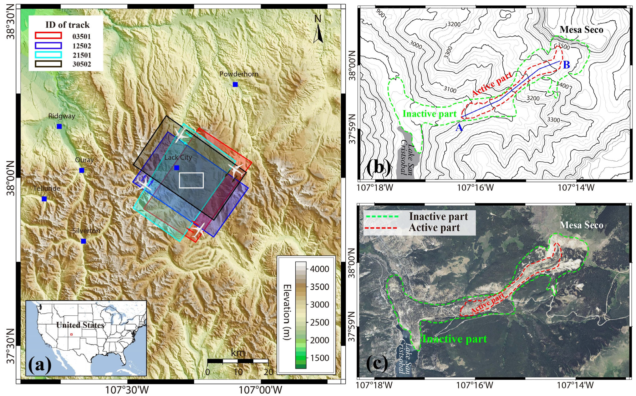
2.1. The Slumgullion Landslide

The Slumgullion landslide, as a well-known ancient landslide, is located in southwestern Colorado, United States [27]. As shown in Figure 1, it consists of two parts: the currently active part (red dashed curve) and the inactive landslide deposits (green dashed curve). The active part, about 300 m wide and 3.9 km long, covers an area of 1.46 km² and has a volume estimated to be 20 × 10⁶ m³ [32,33]. The Slumgullion landslide originates from a collapse of the scarp on Mesa Seco, and the landslide has a mean slope of about 7.5° with a surface elevation of about 2750~3650 m. As shown in Figure 1b, the elevation of the landslide region is significantly lower than that of the surrounding region, and nearly all of the movement occurs by sliding along the shear zones. Because of its flowlike surface morphology, the Slumgullion landslide has historically been called an earth flow [29]. According to the former studies [34,35], the material of this landslide is mainly composed of tertiary basalt, rhyolite, and weathering products including clay, silt, and volcaniclastic rock. A series of geological and kinematic features, including tensile cracks, scarps, depressions, flank ridges, etc., were formed during the landslide movement. The most peculiar fact is its active history within which the younger active part has likely been sliding continuously for about 300 years and the older inactive part has failed at least three times during the past 1300 years [28,29]. The mechanism of its permanent motion and future evolutionary trends have caught the eye of researchers.

In the study of kinetic mechanisms, several techniques have been used to reveal the motion of the Slumgullion landslide. Smith (1993) applied aerial photogrammetry to measure the deformation rates of different parts of the landslide [36]. Based on a Global Positioning System (GPS) and extensometer, some researchers further studied the relation between the motion and regional hydrology (from several years to hours) of the Slumgullion landslide [30,35,37,38,39]. Long-term observations indicate that the motion of the Slumgullion landslide has significant seasonal variations, with a peak in velocity between spring and summer, and is influenced by snowmelt and rainfall [30,35]. The hourly observations reveal that daily accelerations of the landslide are related to atmospheric tides [37]. These studies indicated that several factors (i.e., snowmelt and precipitation) affect the porewater pressures which have effective control of the hourly and seasonal movement of the Slumgullion landslide. With the increase in SAR images in this region, researchers began applying POT [40,41] or D-InSAR [42,43] to obtain the surface displacements of the Slumgullion landslide. For example, Delbridge et al. [44] applied D-InSAR to estimate the three-dimensional (3D) deformations and the depth of the Slumgullion landslide based on UAVSAR data from four tracks. Wang et al. [45] used the time-series deformation derived via the POT method to obtain the kinematic parameters (i.e., linear and seasonal velocities), and revealed the relationships between landslide motion, geological, and meteorological conditions. Subsequently, Hu et al. [46,47,48] also studied the landslide motion and internal structure using the POT and D-InSAR methods. These studies have demonstrated the capacity of SAR to measure landslide deformations and understand the mechanisms affecting their motion. Nevertheless, much remains to be studied about the mass wasting processes and control factors of the Slumgullion landslide, specifically for the changes in the surface mass distribution during evolution.

2.2. SAR Images and Ancillary Datasets

In this study, the UAVSAR dataset is used to estimate the spatial-temporal displacement field of the Slumgullion landslide. As an airborne SAR interferometry system, UAVSAR is deployed by Jet Propulsion Laboratory to acquire L band (wavelength, ~24 cm) SAR images. It was designed from the ground up as a miniaturized polarimetric radar for single-pass and repeat-pass interferometry, with options for along-track interferometry and additional operating frequencies. For robust repeat-pass interferometry, the UAVSAR employs a Precision Autopilot capability to control aircraft position, which can make the spatial baseline of UAVSAR less than 10 m [49]. In addition, the UAVSAR uses an electronically steered flush-mounted antenna that is pointed in the desired direction based on real-time attitude angle measurement [50]. It can ensure that the antenna look directions are identical within a fraction of the beamwidth. Nominally, the system flown at an altitude of 12.5 km covers a swath of about 20 km, with the incidence angles ranging from 25° to 65°. As

Table 1. Parameters of UAVSAR datasets.

Track ID	03501	12502	21501	30502
Heading	34.96°	124.94°	215.04°	305.06°
Observation direction	NW across landslide	NE parallel landslide	SE across landslide	SW parallel landslide
Spacing (azi × rng)	0.60 m × 1.67 m	0.60 m × 1.67 m	0.60 m × 1.67 m	0.60 m × 1.67 m
Look angle	26.97°~69.86°	30.27°~69.82°	27.03°~69.43°	29.64°~69.22°
Number of images	30	30	29	33

shows, the single-look-complex (SLC) data of UAVSAR has a pixel spacing of 1.67 m and 0.60 m in the range and azimuth direction, respectively. The UAVSAR can collect full-polarimetric airborne SAR data, and only HH (horizontal transmission and reception) polarization was used in this study. A detailed descriptions involved in the UAVSAR can be found in the relevant literature [49,50].

Compared with spaceborne SAR, UAVSAR is more agile and convenient to enable acquiring multi-aspect/multi-angular observations in the same area, which facilitates the retrieval of the 3D displacement field of the target region. In the Slumgullion landslide, 122 scenes of UAVSAR images are collected in 33 distinct acquisition times (Figure 2) during the period from 12 August 2011 to 10 October 2018. Due to snow-covered from January to March, the UAVSAR images in the Slumgullion landslide were acquired annually from April to December. These images were acquired from four tracks (ID: 03501, 12502, 21501, and 30502, as shown in Figure 1a), for which the heading directions of adjacent tracks (Table 1) were perpendicular to each other. There are at least three images acquired with different trajectories at each acquisition time. Detailed parameters and coverage for each track are shown in Table 1 and Figure 1 and Figure 2.

Additionally, we also collected the 1/3 arc sec Digital Elevation Model (DEM) from the U.S. Geological Survey (USGS) National Elevation Dataset (NED) in the Slumgullion landslide. The DEM of the Slumgullion landslide, for which metadata was acquired on 10 August 2018, is used to estimate the slope of the landslide. As described by Gesch et al. [51], the mean accuracy of the slope derived using the USGS NED is approximately 0.77°. The high-accuracy slope contributes to the accurate estimation of the landslide mass depletion or accumulation.

3. Methodology

3.1. The POT Method for Mapping Landslide Displacement

The SAR POT method can estimate azimuth and range offsets by SAR amplitude image patch matching independent of coherence and displacement gradients [23,52]. In this paper, we utilized an improved the POT method based on the adaptive normalized cross-correlation (ANCC) POT method [53] to estimate the azimuth $D_{azi}$ and range $D_{rng}$ displacement of the Slumgullion landslide.

According to the motion boundaries, the ANCC POT method generates an optimal irregular matching template composed of pixels with similar moving characteristics (stable or moving). This strategy can improve the robustness and accuracy of the displacement estimation with the SAR POT method. The motion boundaries, which are the key to the ANCC POT method, are extracted using the conventional POT method with a smaller regular matching template. To improve the original process template proposed by Cai et al. [53], we combine the prior landslide boundaries (as identified by Schulz et al. [43]) and traditional POT results to extract the motion boundaries. The detailed principles and steps involved in the ANCC POT can be found in Cai et al. [53]. In view of the range and azimuth pixel spacing of UAVSAR data, we finally use a $128\times 48(azi\times rng)$ matching template with four tracks SAR datasets to measure the landslide displacement. The step of offset estimation is $8\times 2(azi\times rng)$ corresponding to the displacement results with a pixel spacing of 4.80 m and 3.34 m in the azimuth and range direction.

Finally, a time-series processing strategy, which is similar to the SBAS-InSAR [20], is applied to estimate the time-series displacement of the Slumgullion landslide. Following the strategy of forming image pairs with temporal baselines larger than 40 days and less than 400 days, we obtained 393 image pairs from the four tracks of SAR dataset to measure the landslide displacements.

3.2. The 3D Displacement Retrieved from Multi-View Geometries

According to the principle of SAR imaging geometry, the relationship between the 2D displacement ($D_{azi}$ and $D_{rng}$) in the radar coordinate system and the 3D displacement ($D_{east}$, $D_{north}$, and $D_{vertical}$) in the geographic coordinate system can be formulated as

$$\left\{\begin{array}{l}{D}_{azi}+{\delta }_{azi}=D_{north}\mathit{cos}\theta +D_{east}\mathit{sin}\theta \\ D_{rng}+{\delta }_{rng}={D_{north}\mathit{sin}\theta \mathit{sin}\phi -D}_{east}\mathit{cos}\theta \mathit{sin}\phi +D_{vertical}\mathit{cos}\phi \end{array}\right.$$

(1)

where $\phi$ and $\theta$ are the incidence angle and heading angle, respectively. ${\delta }_{azi}$ and ${\delta }_{rng}$ are the observation error in azimuth and range directions, respectively. The introduction of additional view geometries implies the addition of further constraints with the other two conditional equations. Therefore, the 3D displacement can be estimated by combining two or more different view geometries under the least square framework [54].

As Table 1 shows, the UAVSAR images covering the Slumgullion landslide were acquired from four tracks (ID: 03501, 12502, 21501, and 30502), for which the heading direction was perpendicular to each adjacent track. A single track can provide two conditional equations. However, the 2D displacements ($D_{azi}$ and $D_{rng}$) coming from two paralleled tracks (03501 and 21501; 12502 and 30502) have a similar viewing geometry and cannot resolve the 3D displacement. In fact, at least two perpendicular tracks are necessary to resolve the 3D displacement of the Slumgullion landslide. Fortunately, the UAVSAR provided three or four scenes of images acquired from different tracks in each point in time (Table 1). Combining four tracks of UAVSAR data, the mathematical expressions can be simplified as

$$L=BX+V$$

(2)

where

$$L={\left[\begin{array}{ccc}{D}_{azi}^{03501}& D_{rng}^{03501}& \begin{array}{ccc}{D}_{azi}^{12502}& D_{rng}^{12502}& \begin{array}{ccc}{D}_{azi}^{21501}& D_{rng}^{21501}& \begin{array}{cc}{D}_{azi}^{30502}& D_{rng}^{30502}\end{array}\end{array}\end{array}\end{array}\right]}^T,$$

(3)

$$B=\left[\begin{array}{ccc}\mathit{cos}{\theta }^{03501}& \mathit{sin}{\theta }^{03501}& 0\\ \mathit{sin}{\theta }^{03501}\mathit{sin}{\phi }^{03501}& -\mathit{cos}{\theta }^{03501}\mathit{sin}{\phi }^{03501}& \mathit{cos}{\phi }^{03501}\\ \begin{array}{c}\mathit{cos}{\theta }^{12502}\\ \mathit{sin}{\theta }^{12502}\mathit{sin}{\phi }^{12502}\\ \begin{array}{c}\mathit{cos}{\theta }^{21501}\\ \mathit{sin}{\theta }^{21501}\mathit{sin}{\phi }^{21501}\\ \begin{array}{c}\mathit{cos}{\theta }^{30502}\\ \mathit{sin}{\theta }^{30502}\mathit{sin}{\phi }^{30502}\end{array}\end{array}\end{array}& \begin{array}{c}\mathit{sin}{\theta }^{12502}\\ -\mathit{cos}{\theta }^{12502}\mathit{sin}{\phi }^{12502}\\ \begin{array}{c}\mathit{sin}{\theta }^{21501}\\ -\mathit{cos}{\theta }^{21501}\mathit{sin}{\phi }^{21501}\\ \begin{array}{c}\mathit{sin}{\theta }^{30502}\\ -\mathit{cos}{\theta }^{30502}\mathit{sin}{\phi }^{30502}\end{array}\end{array}\end{array}& \begin{array}{c}0\\ \mathit{cos}{\phi }^{12502}\\ \begin{array}{c}0\\ \mathit{cos}{\phi }^{21501}\\ \begin{array}{c}0\\ \mathit{cos}{\phi }^{30502}\end{array}\end{array}\end{array}\end{array}\right],$$

(4)

$$X={\left[\begin{array}{ccc}{D}_{north}& D_{east}& D_{vertical}\end{array}\right]}^T,$$

(5)

$$V={\left[\begin{array}{ccc}{\delta }_{azi}^{03501}& {\delta }_{rng}^{03501}& \begin{array}{ccc}{\delta }_{azi}^{12502}& {\delta }_{rng}^{12502}& \begin{array}{ccc}{\delta }_{azi}^{21501}& {\delta }_{rng}^{21501}& \begin{array}{cc}{\delta }_{azi}^{30502}& {\delta }_{rng}^{30502}\end{array}\end{array}\end{array}\end{array}\right]}^T$$

(6)

where the superscript (e.g., ${\ast }^{03501}$) of parameters indicates the corresponding track of the UAVSAR data. $L$ indicates the landslide displacements estimated using the POT method and $V$ represents the error vector. Then, Equation (2) can be further formed as

$$V=BX-L.$$

(7)

In order to minimize the sum of squares of the residual modulus, it can be expressed as

$$V^{T}PV=min.$$

(8)

The weight matrix $P$ depends on the standard deviations of the 2D displacements estimated using the offset tracking method. Taking the derivative of Equation (8) with respect to $V$:

$$B^{T}PV=0.$$

(9)

Then, substituting the Equation (7) into the Equation (9):

$$B^{T}PBX-B^{T}PL=0.$$

(10)

Therefore, the 3D-displacement $X$ of the Slumgullion landslide can be resolved:

$$X={\left(B^{T}PB\right)}^{-1}{B}^{T}PL.$$

(11)

3.3. The Estimation of Landslide Mass Depletion or Accumulation

The Slumgullion landslide as a translational debris slide has been sliding for hundreds of years. It shows various kinematic features in different regions, which give rise to various changes in the landslide surface during its long-term evolution. The surface mass depletion or accumulation is an important indicator of the kinematic state of the landslide. As a result of this process, the landslide becomes thinner or thicker, which can be quantified based on the 3D-displacement field.

The vertical displacement $D_{vertical}$ (estimated in the Equation (11)) is a projection of landslide movement in the vertical direction. It consists of two components: the down-slope component $D_{v\_slope}$ caused by horizontal movement as well as the component $D_{v\_mass}$ of landslide mass depletion or accumulation. To estimate the landslide mass change distribution, the vertical displacement component $D_{v\_slope}$ needs to be estimated and subtracted from the whole vertical displacement $D_{vitical}.$ The component $D_{v\_slope}$ can be solved based on the following equation:

$$D_{v\_slope}=D_{east}·\left(\frac{\partial h}{\partial e}\right)+D_{north}·\left(\frac{\partial h}{\partial n}\right)$$

(12)

where $D_{east}$ and $D_{north}$ are the landslide displacements in the east (E) direction and north (N) direction, respectively; $\left(\frac{\partial h}{\partial e}\right)$ and $\left(\frac{\partial h}{\partial n}\right)$ are the ground slope in the E direction and N direction, respectively.

Thus, the mass depletion or accumulation distribution of the Slumgullion landslide can be retrieved based on the 3D-displacement field and slope information. This method has been successfully applied in estimating glacier mass balance [55,56]. Thanks to the large landslide coverage and high resolution of UAVSAR data, we were able to apply this method to study the mass wasting of the Slumgullion landslide.

4. Results

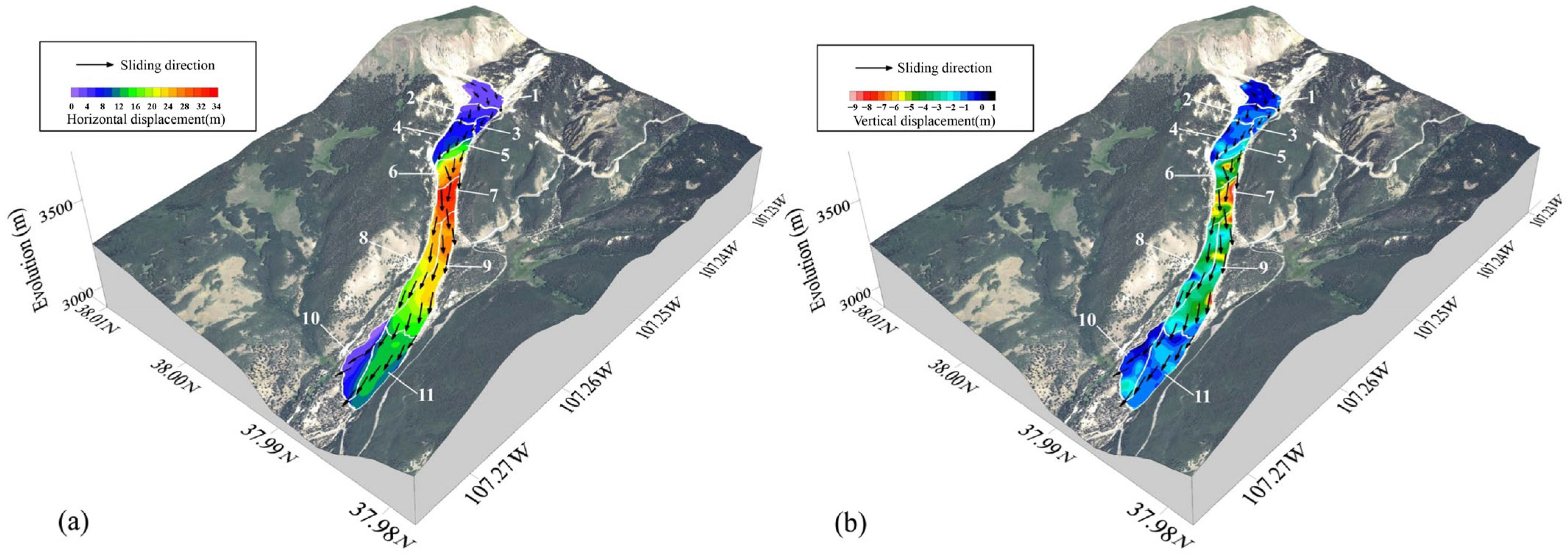
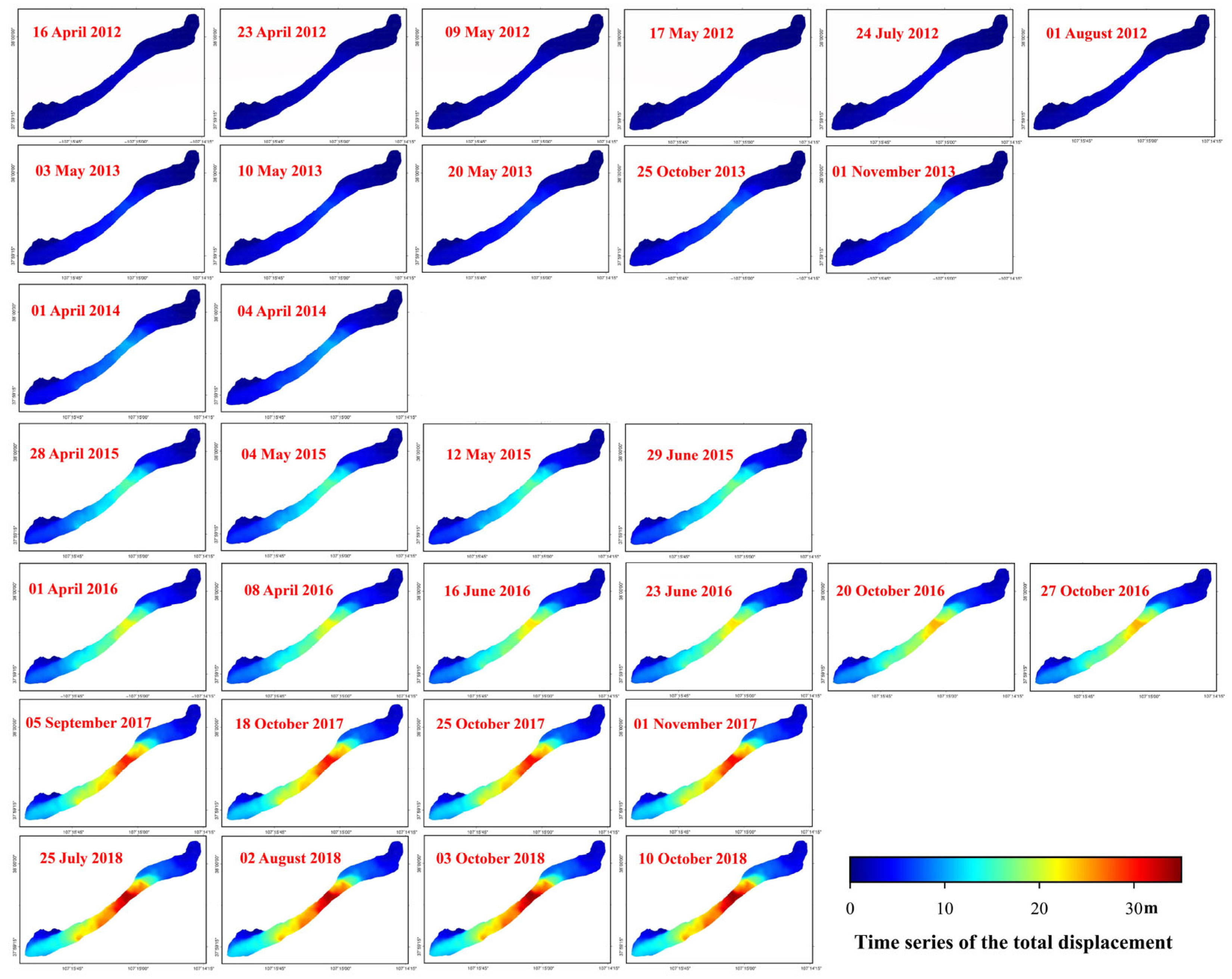
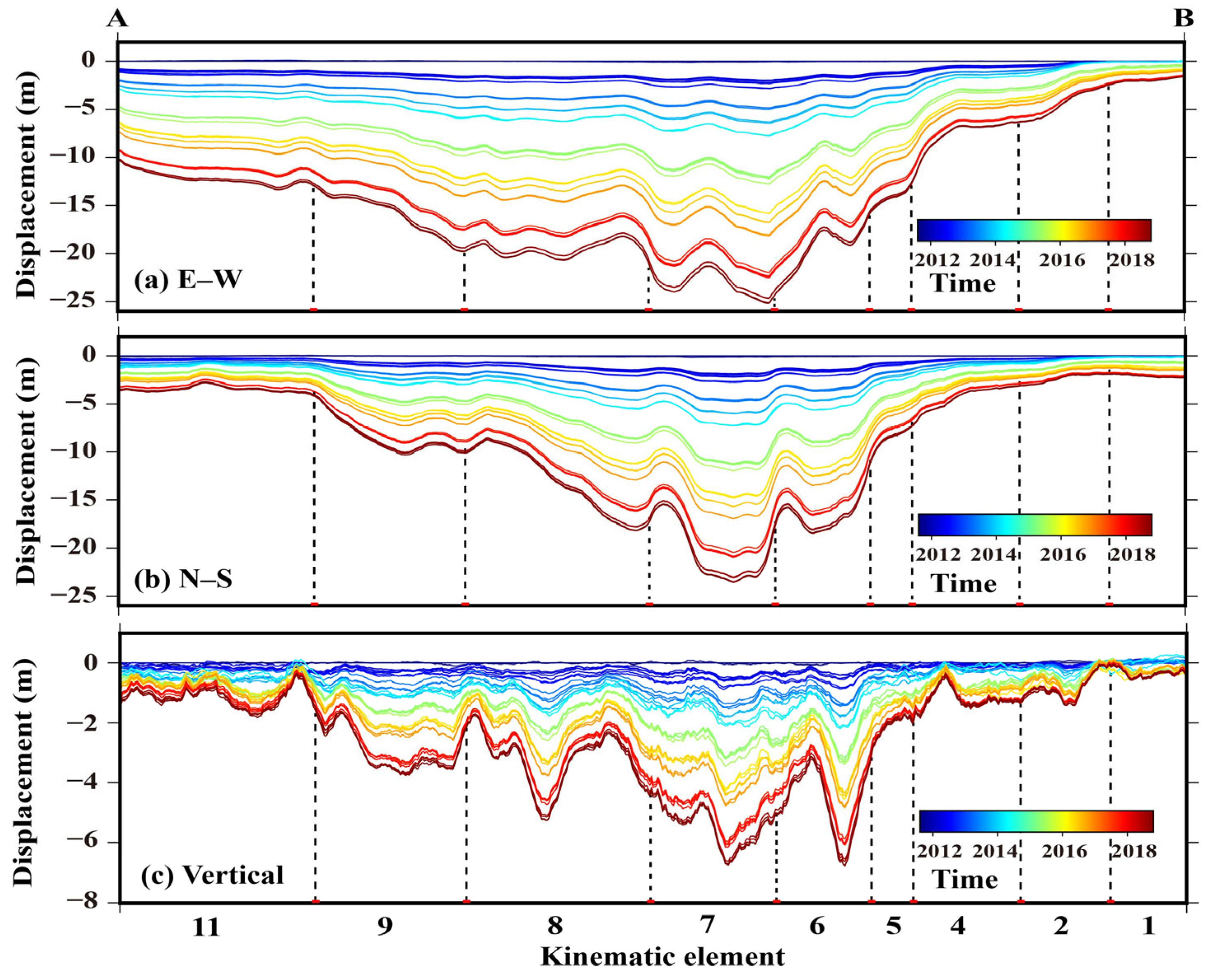
4.1. The Spatial–Temporal Displacement of the Slumgullion Landslide

According to the strategy of image pair formation, we derive the time-series of the 3D displacement field of the Slumgullion landslide at 33 points in time. Figure 3 shows the cumulative horizontal and vertical displacement distribution of the Slumgullion landslide from 12 August 2011 to 10 October 2018. The results suggest that the landslide is shaped like an irregular strip slide from northeast to southwest. The distribution of horizontal displacement shows a clear gradient difference and presents an increasing tendency from both the bottom and the top to the middle area with the decrease of the landslide width. The vertical displacement is irregularly distributed and much smaller than the horizontal displacement.

Schulz et al. [43] divided the Slumgullion landslide into 11 distinct kinematic elements according to the landslide average speeds from August 1985 to August 1990. As Figure 3 shows, the horizontal displacements derived using the ANCC POT method are consistent with these kinematic elements, with significant variation around the element boundaries. In the element 7, the landslide has a maximum total displacement of 35 m during the data spanning period. Large vertical displacements mainly occur in the element 6–9, especially for the element 7, which has a maximum vertical displacement of approximately −9 m. Moreover, some regions in the element 8, 10, and 11 have positive vertical displacements, indicating upward motion in these regions. The maximum positive vertical displacement is approximately 1.5 m and appears at the middle edge of element 8.

Figure 4 shows the time-series of the total displacement of the Slumgullion landslide. The landslide displacements for the same year are shown in the same row. The displacement of the Slumgullion landslide gradually increases with time, with the fastest increase in the neck region. Meanwhile, we can find that the UAVSAR images are not uniformly distributed over time, with the longest interval being more than a year. It indicates that the POT method is able to extract the landslide deformation over a long period of time without the effect of spatial–temporal decorrelation. In addition, we extract a profile AB (blue line in Figure 1b) to show the motion characteristic of the Slumgullion landslide in the spatial–temporal domain. The profile AB is longitudinal through the entire landslide and across almost all kinematic elements (except for the element 3 and 10). Figure 5a–c shows the east–west (E–W), north–south (N–S), and vertical time-series displacement of the profile AB, respectively. The lines with different colors represent the cumulative displacement of the profile AB at the corresponding time. The results indicate that the displacement of the landslide has an approximately steady increasing trend in the temporal domain. In addition, the landslide displacement typically change significantly at the element boundary regions. The E–W displacement sharply increases in the boundary of the element 4 and 5, then gradually reaches the maximum in the element 7. In the boundary regions of the element 5 and 6, the N–S displacement has a significant increase but only a small increase in the E–W displacement. It indicates that the sliding direction mildly turns towards the north. Similarly, the vertical displacement also shows a significant change at the element boundary regions.

Additionally, Figure 6 shows the average root-mean-square errors (RMSEs) of the displacement estimated by the ANCC POT method. The RMSEs of the E–W and N–S displacements range from approximately 0.04 to 0.06 m in most areas, which is approximately less than the precision of 1/10 pixel (0.06 m) in the azimuth direction. Because the estimation of vertical displacements only depends on the observations in range direction which approximate the precision of 1/10 pixel (0.16 m), the RMSEs of the vertical displacements range from approximately 0.12 to 0.16 m. Since the landslide reached a maximum displacement of 35 m during the data spanning period, the accuracy of the displacement field is adequate.

4.2. The Mass Depletion or Accumulation in the Slumgullion Landslide

Based on the 3D-displacement fields and slope information, we reveal the distribution of surface mass change in the Slumgullion landslide. Figure 7 shows the landslide mass depletion or accumulation velocity from August 2011 to October 2018. Negative velocity values indicate mass depletion and landslide thinning, while positive velocity values indicate mass accumulation and landslide thickening. To distinctly show the landslide mass change, we extract a profile AB to show the surface elevation and the time-series of landslide thinning or thickening with expanding twenty-fold (upper-left subgraph in Figure 7). The result indicates that the top (the element 1–4) of the slumgullion landslide is relatively stable and has a mass depletion or accumulation range of about ±1 m. Then, the landslide mass change velocity increases with the increment of the slide velocity in the middle of the landslide.

In the element 6, the landslide has a significant thinning tendency with a max mass depletion velocity of −0.15 cm/day. According to the vertical displacement distribution (as shown in Figure 3b), we can also observe an indication that the vertical displacement significantly increases in a delta-shaped region of the element 6. As shown in the upper-left subgraph of Figure 7, this delta-shaped region has a maximum mass depletion of about −3.65 m during the data spanning period. In the element 7–9, the landslide alternates mass depletion and accumulation bands. The range of mass depletion or accumulation range is approximately from −3 m to 3 m. In the element 10–11, the landslide mainly shows a thickening tendency, as the sliding velocity gradually decreases and the landslide mass accumulates in this area. The thickening of the landslide toe is also verified by [32,38]. The RMSEs of the mass depletion or accumulation (Figure 6d) range from approximately 0.12 to 0.18 m in most areas, which approximate the RMSEs of the vertical displacement. In the neck area, the RMSEs for the mass depletion or accumulation increase to 0.20–0.27 m, as the relatively large horizontal displacements enlarge the effect of the slope errors.

5. Discussion

5.1. The Surface Mass Balance of the Slumgullion Landslide

As mentioned above, the currently active part of the Slumgullion landslide has likely been sliding for hundreds of years. A key issue concerns how the landslide mass wastes during evolution. Previous studies mainly focus on the landslide surface displacements and their influencing factors and rarely pay attention to the surface mass depletion or accumulation, which is an important indicator of landslide kinematic state and future evolutionary trends. Therefore, we estimate the landslide mass volume change in each part of the Slumgullion landslide to analyze the mass wasting process.

Figure 8 shows the mass wasting volume of the 11 elements of the Slumgullion landslide. The results indicate that the whole active part of the Slumgullion landslide approximately loses material with a volume of 1.27 $\times$ 10⁵ m³ during the period from August 2011 to October 2018. According to Parise and Guzzi [33], the activity of the Slumgullion landslide has a volume estimated to be 20 × 10⁶ m³. In other words, the landslide was roughly in balance overall, with the volume of material loss during the data spanning period accounting for about 0.63$\%$ of the total volume of the activity. We infer that the main reason for the subtle loss of mass of the active part is the advance of the landslide toe. Hu et al. [46] indicated that the landslide toe had moved forward about 40 m between 1911 and 2015. The advance of the landslide toe is not derived under the ANCC POT method, and results in an underestimation of the mass accumulation in the landslide toe.

Upon further analysis, the landslide mass is losing on the top and middle of the landslide but is accumulating at the landslide toe. The element 1, which is the beginning of the landslide active part, is a relatively large mass depletion region at the top. The element 2 and 4 are transit zones and are basically in balance. The neck area (element 5–7) is the most active region of the landslide and has the maximal mass depletion in the whole landslide. The velocity of the landslide increases from 0.3 cm/day in the element 4 to 0.6 cm/day in the element 5, to 1.0 cm/day in the element 6, and finally to 1.3 cm/day in the element 7. The larger mass depletion in this area indicates that the decrease in landslide width is far from being the only factor contributing to the sharp increment in landslide velocity. There is another factor that can make an important contribution to the velocity increment in the landslide neck area. The landslide toe (element 10–11) is the only mass accumulation region in the landslide. The material sliding from the middle and top thickens the toe of the landslide and pushes the toe boundary forward. The element 10 is located in the northwest of the landslide toe and deviates from the main sliding direction. As a result, the landslide mass accumulates mainly in the element 11 and secondarily in the element 10.

In summary, the Slumgullion landslide is roughly in balance overall during the data spanning period, with surface mass accumulation in the landslide toe and depletion in the top and middle area. Mass accumulation in the landslide toe results in an increase in the resistive force, and the mass depletion in the upper and middle area results in a decrease in the driving force. This result is convincing evidence to explain why the Slumgullion landslide velocity slowly decreases, and we further infer that the landslide should eventually tend to stabilize in the future.

5.2. The Effect of Geological Structure on Landslide Mass Wasting Process

As shown by the above results, the Slumgullion landslide has complex kinematic features in the spatial domain. These kinematic features are controlled by a variety of factors, such as geological structure. It is helpful to understand the evolutionary mechanism and analyze the effect of the types and distribution of structures on the mass wasting process of landslide.

Figure 9 shows the distribution of the horizontal and vertical velocities of the Slumgullion landslide. The geological structures mapped by Fleming et al. [32] are covered on the velocity map to observe the structures’ influence on the landslide motion. As Figure 9 shows, numerous normal faults are located on the top (element 1–4) of the Slumgullion landslide, but the landslide velocity has little change among these normal faults. The results show that these normal faults at the top of the active part do not show a significant effect on the landslide. With the mass depletion (Figure 8), the top of the landslide should tend to be stable if the headscarp cannot resupply material.

In the middle part, the boundaries of the velocity change gradient are approximately consistent with the distribution of the structures. The elements 4–7 are separated by three large normal faults. These normal faults significantly increase the sliding velocity, and the sliding mass derived from the upper area is not sufficient to support mass balance. Therefore, the Slumgullion landslide has a larger local mass depletion in the neck area (Figure 8). This finding verifies the above analysis that the decrease in landslide width is far from the only factor to the sharp increment of the landslide velocity, and these normal faults also contribute significantly to the velocity increment in the landslide neck area. With the stabilization of the upper landslide, it is likely that the neck area generates a larger scarp and becomes a fresh beginning of the active part.

In the toe of the landslide, a series of thrust faults increase the resistive force and decrease the velocity in this area. Also, a large strike–slip fault separates the element 10 and 11. This strike–slip fault results in a visible difference in the horizontal velocity between the two elements but has little effect on the vertical velocity. The same situation occurs in a strike–slip fault between the boundaries of the element 4 and 5. This phenomenon indicates that strike–slip fault mainly changes the sliding direction of material but has little effect on the vertical motion.

Furthermore, we obtain two rectangle regions A and B (as shown in Figure 9) to observe the detailed distributions of structures and surface mass change. The rectangle-shaped area A, located at the neck of the landslide, is the fastest-moving area of the Slumgullion landslide. The results indicate that the rectangle region A is mainly a mass depletion region, but there are some local mass accumulation regions. The zone center is the largest mass depletion region of the Slumgullion landslide with a mass depletion of about −3.65 m during the data spanning period. A representative mass accumulation area (marked by a’ in Figure 9) in this region is the lower-left portion, which is like a ‘funnel-shaped’ constructed by a series of structures. These structures constrain the material concentrating and accumulating into the a’ area.

In the rectangle B, the mass depletion and accumulation occur alternately as banding. We also observe an unusual mass accumulation in the lower-left portion (marked by b’ in Figure 9). A small normal fault divides b’ area into two parts, an upper part with mass depletion and a lower part with mass accumulation. Normal faults accelerate the sliding of material from the upper part and the accumulation in the lower part. These two distinct parts have comparable area and mass change velocities and approximately constitute a local mass balance.

Based on the above analysis, the distribution of structures could well explain some unique mass depletion or accumulation in the Slumgullion landslide. Geological structures have a considerable influence on the mass wasting process of the Slumgullion landslide.

6. Conclusions

As a well-known ancient landslide, the current active part of the Slumgullion landslide has likely been sliding for approximately 300 years. Its permanent motion and evolutionary processes have attracted the attention of many researchers. In this study, we present an adaptive POT method with multi-track UAVSAR dataset to estimate the spatial–temporal 3D displacement of the Slumgullion landslide. Then, we further reveal the distribution of the mass depletion or accumulation on the landslide surface, and analyze the relationship between landslide motion and geological structures. Our major findings are summarized as follows.

First, the Slumgullion landslide had a spatially variable displacement, with the velocity increasing from approximately 0.3 cm/day in the upper to 1.3 cm/day in the neck area, and finally decreasing to 0.5 cm/day in the toe. The distribution characteristics were consistent with the kinematic elements identified in the previous study.

Second, the slumgullion landslide was roughly in balance overall during the interval time, with surface mass accumulation approximately 3 m in the landslide toe and depletion approximately ranging from −1 to −3 m in the top and middle area. This finding supports the inference that the Slumgullion landslide velocity will gradually decrease and the landslide should eventually tend to be stabilize.

Third, we find that the distribution of structures can well explain some of the unique mass wasting in the Slumgullion landslide. In particular, the results verified that the sharp velocity increment in the neck area is controlled by several normal faults.

Overall, this study provides an insight into the relationship between the landslide motion, mass volume change, and geological structure of the Slumgullion landslide. Although the UAVSAR images during August 2011–October2018 were used to study the landslide motion, the data spanning period is too short compared to the long history of the landslide. Future research explores multi-source data with a long spanning period to study the long-term evolution of the Slumgullion landslide.

References

1. Petley, D. Global patterns of loss of life from landslides. Geology 2012, 40, 927–930. [Google Scholar] [CrossRef]
2. Nappo, N.; Peduto, D.; Mavrouli, O.; van Westen, C.J.; Gullà, G. Slow-moving landslides interacting with the road network: Analysis of damage using ancillary data, in situ surveys and multi-source monitoring data. Eng. Geol. 2019, 260, 105244. [Google Scholar] [CrossRef]
3. Gong, W.; Juang, C.H.; Wasowski, J. Geohazards and human settlements: Lessons learned from multiple relocation events in Badong, China–Engineering geologist’s perspective. Eng. Geol. 2021, 285, 106051. [Google Scholar] [CrossRef]
4. Liu, X.; Zhao, C.; Zhang, Q.; Lu, Z.; Li, Z.; Yang, C.; Zhu, W.; Liu-Zeng, J.; Chen, L.; Liu, C. Integration of Sentinel-1 and ALOS/PALSAR-2 SAR datasets for mapping active landslides along the Jinsha River corridor, China. Eng. Geol. 2021, 284, 106033. [Google Scholar] [CrossRef]
5. Aryal, A.; Brooks, B.A.; Reid, M.E. Landslide subsurface slip geometry inferred from 3-D surface displacement fields. Geophys. Res. Lett. 2015, 42, 1411–1417. [Google Scholar] [CrossRef]
6. Baum, R.L.; Messerich, J.; Fleming, R.W. Surface deformation as a guide to kinematics and three-dimensional shape of slow-moving, clay-rich landslides, Honolulu, Hawaii. Environ. Eng. Geosci. 1998, 4, 283–306. [Google Scholar] [CrossRef]
7. Keefer, D.K.; Larsen, M.C. Assessing landslide hazards. Science 2007, 316, 1136–1138. [Google Scholar] [CrossRef]
8. Samsonov, S.; Dille, A.; Dewitte, O.; Kervyn, F.; d’Oreye, N. Satellite interferometry for mapping surface deformation time series in one, two and three dimensions: A new method illustrated on a slow-moving landslide. Eng. Geol. 2020, 266, 105471. [Google Scholar] [CrossRef]
9. Guo, Z.; Chen, L.; Gui, L.; Du, J.; Yin, K.; Do, H.M. Landslide displacement prediction based on variational mode decomposition and WA-GWO-BP model. Landslides 2020, 17, 567–583. [Google Scholar] [CrossRef]
10. Guo, Z.; Chen, L.; Yin, K.; Shrestha, D.P.; Zhang, L. Quantitative risk assessment of slow-moving landslides from the viewpoint of decision-making: A case study of the Three Gorges Reservoir in China. Eng. Geol. 2020, 273, 105667. [Google Scholar] [CrossRef]
11. Macfarlane, D.F. Observations and predictions of the behaviour of large, slow-moving landslides in schist, Clyde Dam reservoir, New Zealand. Eng. Geol. 2009, 109, 5–15. [Google Scholar] [CrossRef]
12. Song, K.; Wang, F.; Yi, Q.; Lu, S. Landslide deformation behavior influenced by water level fluctuations of the Three Gorges Reservoir (China). Eng. Geol. 2018, 247, 58–68. [Google Scholar] [CrossRef]
13. Zhong, C.; Liu, Y.; Gao, P.; Chen, W.; Li, H.; Hou, Y.; Nuremanguli, T.; Ma, H. Landslide mapping with remote sensing: Challenges and opportunities. Int. J. Remote Sens. 2020, 41, 1555–1581. [Google Scholar] [CrossRef]
14. Ding, C.; Feng, G.; Liao, M.; Tao, P.; Zhang, L.; Xu, Q. Displacement history and potential triggering factors of Baige landslides, China revealed by optical imagery time series. Remote Sens. Environ. 2021, 254, 112253. [Google Scholar] [CrossRef]
15. Jaboyedoff, M.; Oppikofer, T.; Abellán, A.; Derron, M.H.; Loye, A.; Metzger, R.; Pedrazzini, A. Use of LIDAR in landslide investigations: A review. Nat. Hazards 2012, 61, 5–28. [Google Scholar] [CrossRef]
16. Massonnet, D.; Feigl, K.L. Radar interferometry and its application to changes in the Earth’s surface. Rev. Geophys. 1998, 36, 441–500. [Google Scholar] [CrossRef]
17. Colesanti, C.; Wasowski, J. Investigating landslides with space-borne Synthetic Aperture Radar (SAR) interferometry. Eng. Geol. 2006, 88, 173–199. [Google Scholar] [CrossRef]
18. Wasowski, J.; Bovenga, F. Investigating landslides and unstable slopes with satellite Multi Temporal Interferometry: Current issues and future perspectives. Eng. Geol. 2014, 174, 103–138. [Google Scholar] [CrossRef]
19. Rosen, P.A.; Hensley, S.; Joughin, I.R.; Li, F.K.; Madsen, S.N.; Rodriguez, E.; Goldstein, R.M. Synthetic aperture radar interferometry. Proc. IEEE 2000, 88, 333–382. [Google Scholar] [CrossRef]
20. Berardino, P.; Costantini, M.; Franceschetti, G.; Iodice, A.; Pietranera, L.; Rizzo, V. Use of differential SAR interferometry in monitoring and modelling large slope instability at Maratea (Basilicata, Italy). Eng. Geol. 2003, 68, 31–51. [Google Scholar] [CrossRef]
21. Ferretti, A.; Prati, C.; Rocca, F. Permanent scatterers in SAR interferometry. IEEE Trans. Geosci. Remote Sens. 2001, 39, 8–20. [Google Scholar] [CrossRef]
22. Bechor, N.B.; Zebker, H.A. Measuring two-dimensional movements using a single InSAR pair. Geophys. Res. Lett. 2006, 33, L16311. [Google Scholar] [CrossRef]
23. Michel, R.; Avouac, J.P.; Taboury, J. Measuring ground displacements from SAR amplitude images: Application to the Landers earthquake. Geophys. Res. Lett. 1999, 26, 875–878. [Google Scholar] [CrossRef]
24. Cai, J.; Zhang, L.; Dong, J.; Wang, C.; Liao, M. Polarimetric SAR pixel offset tracking for large-gradient landslide displacement mapping. Int. J. Appl. Earth Obs. Geoinf. 2022, 112, 102867. [Google Scholar] [CrossRef]
25. Zheng, W.; Hu, J.; Lu, Z.; Hu, X.; Sun, Q.; Liu, J.; Zhu, J.; Li, Z. Enhanced Kinematic Inversion of 3-D Displacements, Geometry, and Hydraulic Properties of a North-South Slow-Moving Landslide in Three Gorges Reservoir. J. Geophys. Res. Solid Earth 2023, 128, e2022JB026232. [Google Scholar] [CrossRef]
26. Zheng, W.; Hu, J.; Liu, J.; Sun, Q.; Li, Z.; Zhu, J.; Wu, L. Mapping complete three-dimensional ice velocities by integrating multi-baseline and multi-aperture InSAR measurements: A case study of the Grove mountains area, East Antarctic. Remote Sens. 2021, 13, 643. [Google Scholar] [CrossRef]
27. Cruden, D.M.; Varnes, D.J. Landslide types and processes, special report, transportation research board, national academy of sciences. Spec. Rep. Natl. Res. Counc. Transp. Res. Board 1996, 247, 76. [Google Scholar]
28. Madole, R.F. Preliminary chronology of the Slumgullion landslide, Hinsdale County, Colorado. In The Slumgullion Earth Flow: A Largescale Natural Laboratory; Varnes, D.J., Savage, W.Z., Eds.; U.S. Geological Survey Bulletin: Reston, VA, USA, 1996; Volume 2130, pp. 5–7. [Google Scholar]
29. Varnes, D.J.; Savage, W.Z. (Eds.) The Slumgullion Earth Flow: A Large-Scale Natural Laboratory; US Government Printing Office: Washington, DC, USA, 1996. [Google Scholar]
30. Coe, J.A.; Ellis, W.L.; Godt, J.W.; Savage, W.Z.; Savage, J.E.; Michael, J.A.; Kibler, J.D.; Powers, P.S.; Lidke, D.J.; Debray, S. Seasonal movement of the Slumgullion landslide determined from Global Positioning System surveys and field instrumentation, July 1998–March 2002. Eng. Geol. 2008, 68, 67–101. [Google Scholar] [CrossRef]
31. Madson, A.; Fielding, E.; Sheng, Y.; Cavanaugh, K. High-resolution spaceborne, airborne and in situ landslide kinematic measurements of the slumgullion landslide in Southwest Colorado. Remote Sens. 2019, 11, 265. [Google Scholar] [CrossRef]
32. Fleming, R.W.; Baum, R.L.; Giardino, M. Map and Description of the Active Part of the Slumgullion Landslide, Hinsdale County, Colorado; Investigations Series Map I-2672; U.S. Geological Survey: Reston, VA, USA, 1999. [Google Scholar] [CrossRef]
33. Parise, M.; Guzzi, R. Volume and Shape of the Active and Inactive Parts of the Slumgullion Landslide, Hinsdale County, Colorado; US Department of the Interior, US Geological Survey: Reston, VA, USA, 1992; p. 29. [Google Scholar] [CrossRef]
34. Chleborad, A.F.; Diehl, S.F.; Cannon, S.H. Geotechnical properties of selected materials from the Slumgullion landslide. In The Slumgullion Earth Flow: A Large-Scale Natural Laboratory; Varnes, D.J., Savage, W.Z., Eds.; U.S. Geological Survey Bulletin: Reston, VA, USA, 1996; Volume 2130, pp. 67–71. [Google Scholar]
35. Schulz, W.H.; McKenna, J.P.; Biavati, G.; Kibler, J.D. Characteristics of Slumgullion landslide inferred from subsurface exploration, in-situ and laboratory testing, and monitoring. In Proceedings of the 1st North American Landslide Conference, Vail, CO, USA, 3–8 June 2007; pp. 3–8. [Google Scholar]
36. Smith, W.K. Photogrammetric Determination of Movement on the Slumgullion Slide, Hinsdale County, Colorado 1985–1990; US Department of the Interior, US Geological Survey: Reston, VA, USA, 1993; pp. 93–597. [Google Scholar] [CrossRef]
37. Schulz, W.H.; Kean, J.W.; Wang, G. Landslide movement in Southwest Colorado triggered by atmospheric tides. Nat. Geosci. 2009, 2, 863–866. [Google Scholar] [CrossRef]
38. Coe, J.A.; McKenna, J.P.; Godt, J.W.; Baum, R.L. Basal-topographic control of stationary ponds on a continuously moving landslide. Earth Surf. Process. Landf. 2009, 34, 264–279. [Google Scholar] [CrossRef]
39. Coe, J.A. Regional moisture balance control of landslide motion: Implications for landslide forecasting in a changing climate. Geology 2012, 40, 323–326. [Google Scholar] [CrossRef]
40. Wang, C.; Mao, X.; Wang, Q. Landslide displacement monitoring by a fully polarimetric SAR offset tracking method. Remote Sens. 2016, 8, 624. [Google Scholar] [CrossRef]
41. Amitrano, D.; Guida, R.; Dell’Aglio, D.; Di Martino, G.; Di Martire, D.; Iodice, A.; Costantini, M.; Malvarosa, F.; Minati, F. Long-term satellite monitoring of the slumgullion landslide using space-borne synthetic aperture radar sub-pixel offset tracking. Remote Sens. 2019, 11, 369. [Google Scholar] [CrossRef]
42. Milillo, P.; Fielding, E.J.; Shulz, W.H.; Delbridge, B.G.; Burgmann, R. COSMO-SkyMed spotlight interferometry over rural areas: The Slumgullion landslide in Colorado, USA. IEEE J. Sel. Top. Appl. Earth Observ. Remote Sens. 2014, 7, 2919–2926. [Google Scholar] [CrossRef]
43. Schulz, W.H.; Coe, J.A.; Ricci, P.P.; Smoczyk, G.M.; Shurtleff, B.L.; Panosky, J. Landslide kinematics and their potential controls from hourly to decadal timescales: Insights from integrating ground-based InSAR measurements with structural maps and long-term monitoring data. Geomorphology 2017, 285, 121–136. [Google Scholar] [CrossRef]
44. Delbridge, B.G.; Delbridge, B.; Fielding, E.J.; Hensley, S.; Schulz, W.H. 3D surface deformation derived from airborne interferometric UAVSAR: Application to the Slumgullion landslide. J. Geophys. Res. Solid Earth 2016, 121, 3951–3977. [Google Scholar] [CrossRef]
45. Wang, C.; Cai, J.; Li, Z.; Mao, X.; Feng, G.; Wang, Q. Kinematic parameter inversion of the slumgullion landslide using the time series offset tracking method with UAVSAR data. J. Geophys. Res. Solid Earth 2018, 123, 8110–8124. [Google Scholar] [CrossRef]
46. Hu, X.; Bürgmann, R.; Schulz, W.H.; Fielding, E.J. Four-dimensional surface motions of the Slumgullion landslide and quantification of hydrometeorological forcing. Nat. Commun. 2020, 11, 2792. [Google Scholar] [CrossRef]
47. Hu, X.; Bürgmann, R. Rheology of a debris slide from the joint analysis of UAVSAR and LiDAR data. Geophys. Res. Lett. 2020, 47, e2020GL087452. [Google Scholar] [CrossRef]
48. Hu, X.; Bürgmann, R.; Fielding, E.J.; Lee, H. Internal kinematics of the Slumgullion landslide (USA) from high-resolution UAVSAR InSAR data. Remote Sens. Environ. 2020, 251, 112057. [Google Scholar] [CrossRef]
49. Hensley, S.; Zebker, H.; Jones, C.; Michel, T.; Muellerschoen, R.; Chapman, B. First deformation results using the NASA/JPL UAVSAR instrument. In Proceedings of the 2009 2nd Asian-Pacific Conference on Synthetic Aperture Radar, Xi’an, China, 26–30 October 2009; pp. 1051–1055. [Google Scholar]
50. Hensley, S.; Wheeler, K.; Sadowy, G.; Jones, C.; Shaffer, S.; Zebker, H.; Miller, T.; Heavey, B.; Chuang, E.; Chao, R.; et al. The UAVSAR instrument: Description and first results. In Proceedings of the 2008 IEEE Radar Conference, Rome, Italy, 26–30 May 2008; pp. 1–6. [Google Scholar]
51. Gesch, D.B.; Oimoen, M.J.; Evans, G.A. Accuracy Assessment of the US Geological Survey National Elevation Dataset, and Comparison with Other Large-Area Elevation Datasets: SRTM and ASTER; US Department of the Interior, US Geological Survey: Sioux Falls, SD, USA, 2014; Volume 1008. [Google Scholar] [CrossRef]
52. Raspini, F.; Bianchini, S.; Moretti, S.; Loupasakis, C.; Rozos, D.; Duro, J.; Garcia, M. Advanced interpretation of interferometric SAR data to detect, monitor and model ground subsidence: Outcomes from the ESA-GMES Terrafirma project. Nat. Hazards 2016, 83, 155–181. [Google Scholar] [CrossRef]
53. Cai, J.; Wang, C.; Mao, X.; Wang, Q. An adaptive offset tracking method with SAR images for landslide displacement monitoring. Remote Sens. 2017, 9, 830. [Google Scholar] [CrossRef]
54. Li, M.; Zhang, L.; Shi, X.; Liao, M.; Yang, M. Monitoring active motion of the Guobu landslide near the Laxiwa Hydropower Station in China by time-series point-like targets offset tracking. Remote Sens. Environ. 2019, 221, 80–93. [Google Scholar] [CrossRef]
55. Gray, L. Using multiple RADARSAT InSAR pairs to estimate a full three-dimensional solution for glacial ice movement. Geophys. Res. Lett. 2011, 38, L05502. [Google Scholar] [CrossRef]
56. Hu, J.; Li, Z.; Li, J.; Zhang, L.; Ding, X.; Zhu, J.; Sun, Q. 3-D movement mapping of the alpine glacier in Qinghai-Tibetan Plateau by integrating D-InSAR, MAI and Offset-Tracking: Case study of the Dongkemadi Glacier. Glob. Planet. Chang. 2014, 118, 62–68. [Google Scholar] [CrossRef]
Figure 1. Overview of the Slumgullion landslide: (a) The landslide location with the background topography derived using the ALOS World 3D (AW3D) Digital Surface Model (DSM). (b) The contour map showing the active (red dashed line) and inactive (green dashed line) boundaries of the landslide. (c) The optical image from Google Earth™. The solid boxes with different colors represent the coverage of four orbit’s SAR images. The airplane directions represent the heading directions of different tracks.
Remotesensing 15 04746 g001
Figure 2. The detailed acquisition time of UAVSAR images. The blue, red, yellow, and purple blocks represent images of the 03501, 12502, 21501, and 30502 track, respectively.
Remotesensing 15 04746 g002
Figure 3. The cumulative horizontal (a) and vertical (b) displacement distribution of the Slumgullion landslide from 12 August 2011 to 10 October 2018. The vertical upward displacement is positive and the sliding direction is represented by the black arrow. The landslide is divided into 11 distinct kinematic elements by the white lines, as identified by Schulz et al. [43].
Remotesensing 15 04746 g003
Figure 4. The time-series of the total displacement of the Slumgullion landslide during the data spanning period.
Remotesensing 15 04746 g004
Figure 5. The cumulative displacement of the profile AB (blue line in Figure 1b) during the data spanning period: (a) E–W displacement; (b) N–S displacement; (c) Vertical displacement. The different colors of lines represent the corresponding times. The positive values indicate eastward, northward, and upward, respectively.
Remotesensing 15 04746 g005
Figure 6. The average RMSEs of the displacement fields and thickness change estimated using the ANCC POT method: (a) The RMSEs of the E–W displacement; (b) The RMSEs of N–S displacement; (c) The RMSEs of the vertical displacement; (d) The RMSEs of the mass depletion or accumulation.
Remotesensing 15 04746 g006
Figure 7. The surface mass depletion or accumulation velocity of the Slumgullion landslide. The upper-left subgraph shows the surface elevation and time-series of landslide mass depletion or accumulation with twenty-fold expansion. The different colors of lines in the upper-left subgraph represent the corresponding times. The 11 distinct kinematic elements are described by the black lines.
Remotesensing 15 04746 g007
Figure 8. The mass wasting volume of the 11 elements of the Slumgullion landslide during the period from August 2011 to October 2018: (a) the spatial distribution of mass wasting volume; (b) the quantitative value of mass wasting volume.
Remotesensing 15 04746 g008
Figure 9. The horizontal and vertical velocity of the Slumgullion landslide covered with principal structures mapped by [32]. Two rectangle areas A and B are selected to show the detailed distribution of the structures and mass depletion or accumulation.
Remotesensing 15 04746 g009