TCUNet: A Lightweight Dual-Branch Parallel Network for Sea–Land Segmentation in Remote Sensing Images

Abstract

Remote sensing techniques for shoreline extraction are crucial for monitoring changes in erosion rates, surface hydrology, and ecosystem structure. In recent years, Convolutional neural networks (CNNs) have developed as a cutting-edge deep learning technique that has been extensively used in shoreline extraction from remote sensing images, owing to their exceptional feature extraction capabilities. They are progressively replacing traditional methods in this field. However, most CNN models only focus on the features in local receptive fields, and overlook the consideration of global contextual information, which will hamper the model’s ability to perform a precise segmentation of boundaries and small objects, consequently leading to unsatisfactory segmentation results. To solve this problem, we propose a parallel semantic segmentation network (TCU-Net) combining CNN and Transformer, to extract shorelines from multispectral remote sensing images, and improve the extraction accuracy. Firstly, TCU-Net imports the Pyramid Vision Transformer V2 (PVT V2) network and ResNet, which serve as backbones for the Transformer branch and CNN branch, respectively, forming a parallel dual-encoder structure for the extraction of both global and local features. Furthermore, a feature interaction module is designed to achieve information exchange, and complementary advantages of features, between the two branches. Secondly, for the decoder part, we propose a cross-scale multi-source feature fusion module to replace the original UNet decoder block, to aggregate multi-scale semantic features more effectively. In addition, a sea–land segmentation dataset covering the Yellow Sea region (GF Dataset) is constructed through the processing of three scenes from Gaofen-6 remote sensing images. We perform a comprehensive experiment with the GF dataset to compare the proposed method with mainstream semantic segmentation models, and the results demonstrate that TCU-Net outperforms the competing models in all three evaluation indices: the PA (pixel accuracy), F1-score, and MIoU (mean intersection over union), while requiring significantly fewer parameters and computational resources compared to other models. These results indicate that the TCU-Net model proposed in this article can extract the shoreline from remote sensing images more effectively, with a shorter time, and lower computational overhead.

1. Introduction

A coastline refers to the boundary line or marginal area between the ocean or lake and the land [1]. Different and debated are the definitions of coastline, because defining the sea–land interface is neither conceptually nor physically simple; one of the conceptually simplest is defined as the boundary between the land surface and the ocean surface [2], also known as an instantaneous coastline, in the field of remote sensing application research. The types of coastline are mainly divided into rocky coasts, sandy coasts, silty coasts, biological coasts, and artificial coastlines. Coastline information is an important basis for the implementation of coastal zone protection and disaster management, the basis for the development and use of marine resources, and an important territorial resource for countries bordering the sea, and plays an significant role in the ecological safety of the ocean [3]. However, at the same time, the extraction of the coastline is a very challenging problem, because it is the land–water boundary of the multi-year average high tide, rather than an instantaneous line [4]. Traditional shoreline extraction methods are mainly manual measurements. However, manual surveying and mapping is associated with issues of labor intensiveness and a lengthy surveying and mapping duration, which consequently lead to a reduced efficiency. Additionally, the influence of human factors [5]; for instance, errors introduced during the process of data collection and variations in subjective judgments and drawing styles among different operators when delineating coastlines; results in disparities in the depiction of the same coastline area on different maps. Collectively, these factors will have an impact on the precise depiction of the coastline. In contrast, remote sensing images have the advantages of a wide coverage, fast information acquisition, high data reliability, fewer constraints caused by the weather, geographic environment and other conditions, free access, etc., which can greatly reduce the cost of surveying and mapping and, therefore, have been commonly used in agricultural development, sea monitoring, and other fields [6,7]. Remote sensing technology has become the main technical means of coastline research, and is widely used in the extraction and monitoring of coastlines.

Coastline extraction methods mainly include threshold segmentation methods [8], edge detection algorithms, object-oriented methods, machine learning methods, and deep learning methods [9]. The threshold segmentation method divides the pixels in an image into two or more categories according to the pixel digital number values, so as to divide the image into different regions. In remote sensing images, the spectral water index (SWI) method is often used; i.e., based on the different reflectance properties of water bodies and non-water bodies in the infrared and visible bands, we calculate certain combinations of bands in the remote sensing image, to distinguish between water bodies and non-water bodies. For example, there is the Normalized Difference Water Index (NDWI) [10] and the Modified Normalized Difference Water Index (MNDWI) [11]. However, threshold-based methods often require thresholds to be set manually, but different images often have large differences, and it is likely that different thresholds will need to be set, making threshold selection difficult and, thus, affecting the final shoreline extraction accuracy. In addition, the coastline region has a complex terrain; there are shadows cast by the surrounding terrain, clouds, vegetation, and other factors, meaning that considering only the spectral differences to distinguish between land and water will make the accuracy lower. Image edge detection algorithms, currently commonly used as edge detection models include the Roberts operator [12], Sobel operator [13], Canny operator [14], and so on. However, the coastline detected by such methods is highly affected by noise, and the noise causes distortion in the edge detection results. Thus, the detected edges are not accurate enough. At the same time, these methods are less efficient, and can only detect the significant edges in the image, and the accuracy of the obtained boundaries is not high [4,15,16]. The object-oriented classification method combines pixels into objects, integrating their interrelationships and spatial distributions, and thereby reducing the interference from internal pixel information, and maximizing the utilization of image information. However, due to the complexity of the steps, processing difficulties, and the difficulty of determining the threshold value of image segmentation, it is difficult to use in a wide range of high-resolution images with many features and information. Many machine learning algorithms extract diverse information based on a variety of data, and use traditional machine learning algorithms, such as random forest [17] or support vector machine (SVM) [18], to extract the shoreline. These algorithms are able to extract the shoreline quickly and efficiently compared to traditional methods. Traditional machine learning methods have certain limitations. For instance, when manually extracting image features as input, and selecting features, it is possible that the complex distinctions between the ocean and land cannot be fully captured, thereby restricting the algorithm’s generalization ability and robustness. Furthermore, machine learning algorithms typically focus only on individual pixel features, neglecting the spatial relationships and contextual information among pixels, leading to insufficient smoothness and accuracy in the segmentation results. As a result, these limitations result in a lack of precision in traditional machine learning methods when extracting complex coastlines from high-resolution images [4,16,19].

Advancements in computer technology and artificial intelligence have generated considerable interest in the application of deep learning techniques, particularly in the domain of computer vision, including, but not limited to, semantic segmentation [20] and object detection [21]. In contrast to other approaches, deep learning models, specifically those based on convolutional neural networks (CNNs) [22], have demonstrated a superior capacity to handle intricate image features, and show robust self-learning capabilities. Long et al. [23] proposed the use of a full convolution network (FCN) to solve the problem that a traditional convolutional neural network (CNN) cannot directly handle variable length inputs and outputs. They used convolutional layers instead of fully connected layers, and used methods such as inverse convolution and up-sampling to reduce the feature maps, which provided new ideas for those who came after them. On this basis, U-Net, proposed by Ronneberger O et al. [24], has been extensively employed in the domain of medical image segmentation. Its innovative architecture and the introduction of jump connections bring new methods for image segmentation research. Furthermore, the domain of semantic segmentation encompasses several classical methods, including SegNet [25], PSPNet [26], the Deeplab series [20,27,28], HRNet [29], and so on. In addition, several researchers have endeavored to integrate CNN methods into land and water segmentation in remote sensing images, which has led to substantial enhancements in the accuracy of shoreline extraction. Li et al. [30] proposed a model called DeepUNet, which is deeper than U-Net, and improves the accuracy by 2% compared to U-Net. Shamsolmoali et al. [31] combined the DenseNet [32] and ResNet [33] to develop RDUNet, which has a better classification accuracy than DeepUNet, DenseNet, and other models. He et al. [34] combined the attention mechanism with the classical UNet network to devise a novel segmentation network for extracting glacial lakes in remote sensing images, which enhances the classification accuracy, as well as achieving clearer boundaries compared to the traditional models.

However, traditional CNN methods capture detailed features of an image only from a local scope, and do not determine the target boundaries from the global level, based on the contextual information of the image. In recent years, Transformer [35] has been migrated to computational vision tasks, showing amazing potential and value. By dividing images into image patches, and applying a self-attention mechanism, global contextual information can be utilized for classification, rather than just local features. This global information processing gives Transformer an advantage over other methods when dealing with large-scale images and complex scenes. The Vision Transformer (ViT), proposed by Dosovitskiy et al. [36], is a transformer-based architecture developed for large-scale image recognition tasks. The fundamental concept behind ViT is to divide the input image into a series of image patches, considering each patch as an element in a sequence. These image patches are transformed into corresponding embedding vectors, through a linear mapping layer, and combined with position coding, to form the input to the Transformer model. By processing these input embedding vectors through multiple Transformer encoder layers, ViT is able to capture the global contextual information in the image and, thus, process image tasks efficiently, with a relatively good performance. Several studies have modified the architecture of ViT for dense prediction tasks. The Pyramid Vision Transformer (PVT) [37] was the first transformer-based model to import the feature pyramid of CNNs. With the pyramid structure capturing the multi-scale features, and the Transformer model achieving global context modelling, PVT has shown a good performance in image classification tasks. Later, a hierarchical attention mechanism was proposed in the Swin Transformer [38], which performs attention computation at multiple scales, thus reducing the computational and memory burden. It is able to handle large-size images with a good scalability and efficiency, achieving an excellent image classification performance. Meanwhile, in the domain of semantic segmentation, segmentation transformers (SETR) [39] employ ViT as a backbone to extract features, while the decoder uses progressive up-sampling to mitigate the noise problem. After four up-sampling operations to obtain the segmentation results subsequently, semantic segmentation transformers (SegFormer) [40] achieved some improvements on STER, by removing positional coding, and introducing convolutional operations, while using a hierarchical encoder structure that outputs multi-scale features and, finally, designed a lightweight decoder, to reduce the computational overhead. These changes further improve its segmentation effect.

However, it has been pointed out [41,42,43] that results based on sheer transformer-based segmentation networks are suboptimal, primarily because transformers are inclined towards global modelling, and lack location awareness. Furthermore, due to the unique self-attention mechanism, and absence of convolutional operations, in Transformer models, they suffer from certain drawbacks in modeling spatial information, expressing local details, preserving image invariance, and maintaining robustness. Consequently, these limitations result in the disruption of image structure, and loss of information. Therefore, many scholars have tried to design methods with better results, by combining the union of CNNs and transformers. TransUNet [41] used a hybrid Vision Transformer structure to stack CNNs and transformers sequentially as an encoder, while the decoder followed the classical UNet, and achieved good results in medical image segmentation. He et al. [44] constructed a novel parallel dual-branch encoder based on TransUNet, using Swin Transformer as a secondary encoder, and the original hybrid Vision Transformer primary encoder, and achieved good segmentation results on hyperspectral images. Chen et al. [45] put forth a dual-branch parallel network for segmentation tasks. In the encoding part, ResNet50 and Swin transformers serve as a dual-branch backbone, to capture the features from the input images, followed by the complete fusion of the extracted information. A new fusion module is proposed during the decoding process for multi-scale feature fusion. The experimental results show that the network maximizes the advantages of both the backbone networks, and improves the accuracy of semantic segmentation tasks related to buildings and water bodies.

Inspired by these works, and in order to solve the problems of complex shoreline extraction and fine water-body identification, in this study, we propose a new two-branch parallel image segmentation network fusing CNN and Transformer, to achieve the accurate segmentation of sea and land in multispectral remote sensing images. The paper primarily contributes via the following four aspects:

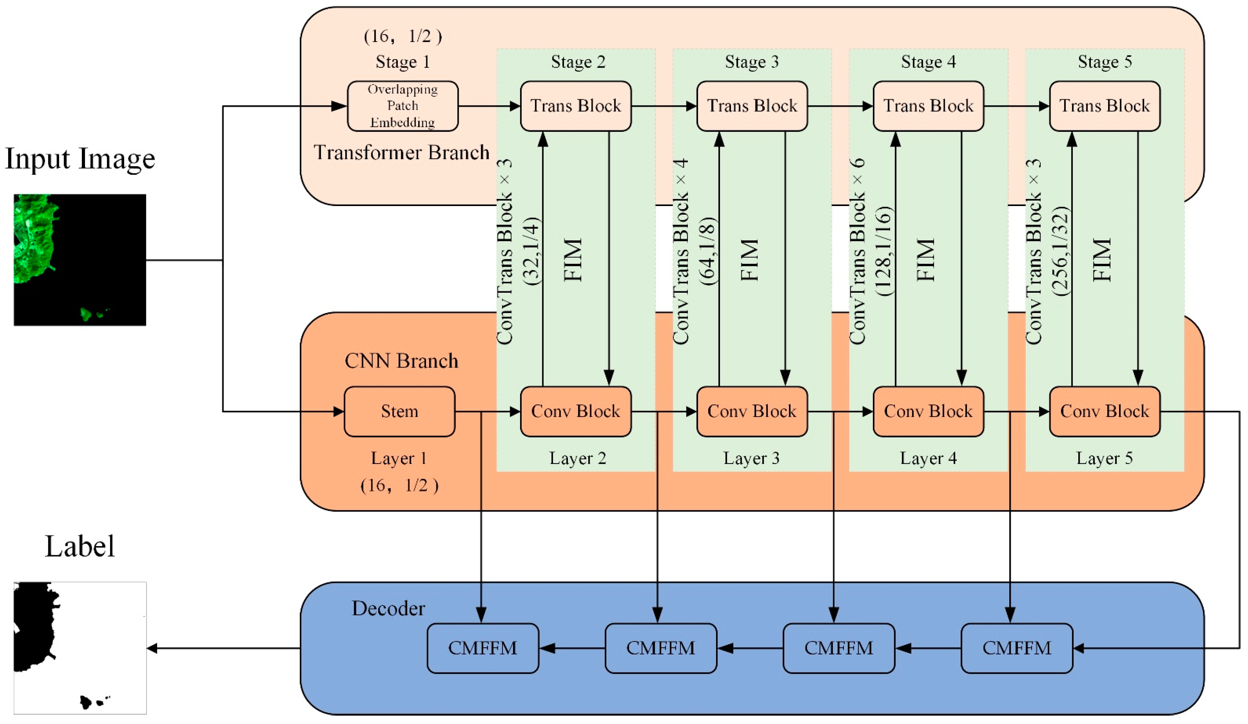
• In this paper, we propose TCUNet, a parallel two-branch image segmentation network fusing CNN and Transformer, to achieve a fine segmentation of land and sea in multispectral remote sensing images.
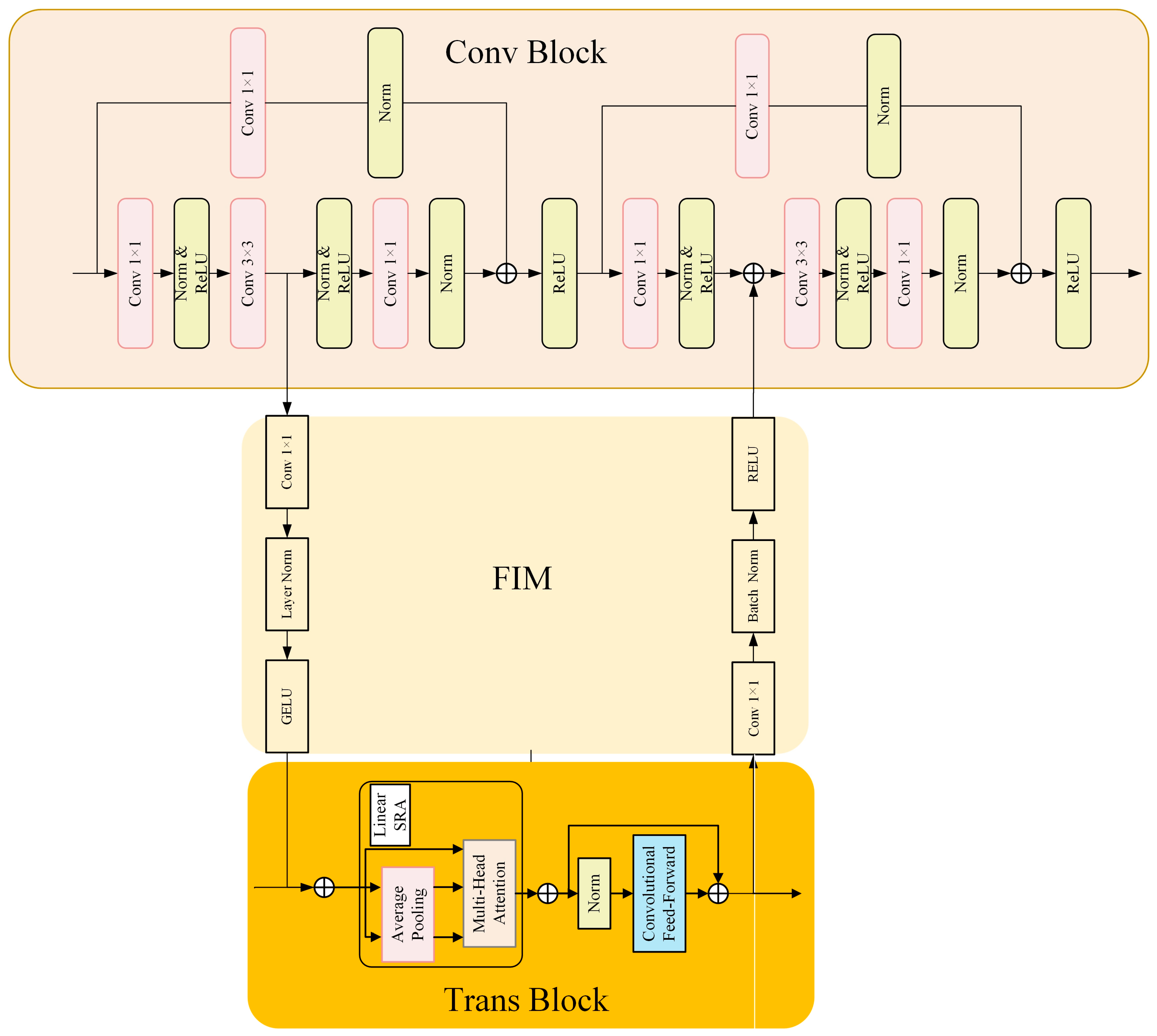
• We design a new lightweight feature interaction module (FIM) to achieve feature exchange and information flow in the dual branch, by embedding it between each coding block in the dual branch, to minimize the semantic gap of the dual branch, enhancing the global representation of the CNN branch, while complementing the local details of the Transformer branch.
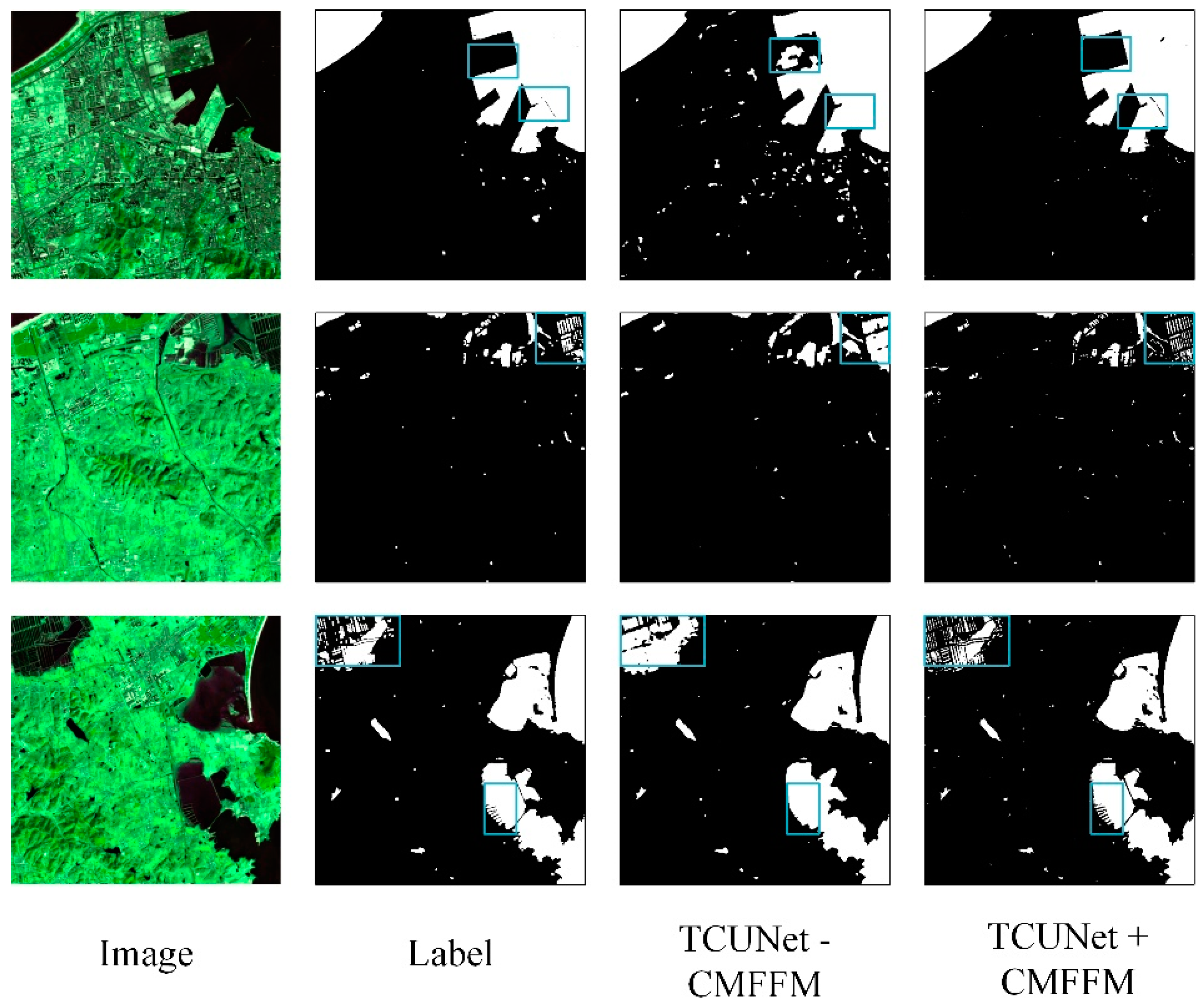
• We propose a cross-scale, multi-source feature fusion module (CMFFM) to replace the decoder block in UNet, to solve the issue of feature inconsistency between different scales, and achieve the fusion of multi-source features at different scales.
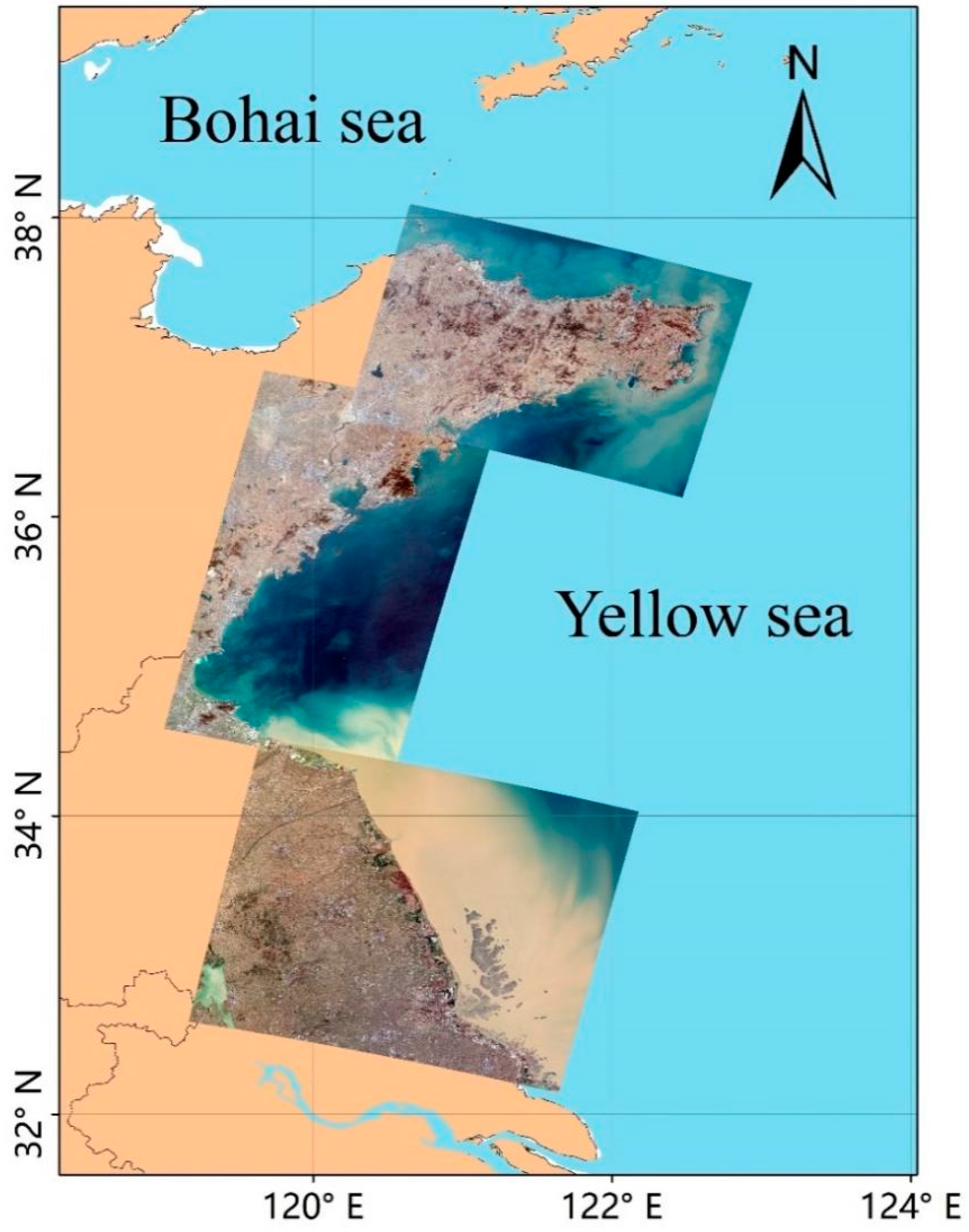
• Based on three Gaofen-6 satellite images produced in February 2023, we constructed a sea–land semantic segmentation dataset, the GF dataset, covering the entire Yellow Sea region of China, which contains 12,600 sheets, each with a size of 512 pixels × 512 pixels. We have made it available for public use.

2. Methods and Materials

2.1. Overall Network Structure

Most of the existing land and sea segmentation models use a convolutional neural network as an encoder to achieve land and sea feature extraction from remote sensing images. Despite being highly effective in local feature extraction, and significantly enhancing the network’s robustness in sea–land segmentation, CNNs extract image features by reusing convolutional and pooling layers, but this results in a limited size of the model’s receptive field. When dealing with large images, the convolution kernel needs to become very large, which increases the computational cost and memory consumption. Convolutional neural networks are, after all, only network structures that focus on local information, and this computational mechanism leads to difficulties in capturing and storing global information over long distances. Numerous transformer-based backbone networks have emerged, integrating the self-attention mechanism to effectively capture global contextual information, and address the limitations of CNN in recent years. However, compared to CNN, transformer-based models cannot fully utilize the local features of the image.

To address this limitation, we propose a novel parallel semantic segmentation network based on a transformer and CNN, to extract comprehensive global information and intricate local details between the target and background for sea–land segmentation tasks. The network architecture, as illustrated in Figure 1, comprises a CNN branch, a Transformer branch, a feature interaction module (FIM) and a cross-scale multi-level feature fusion module (CMFFM), which are described in detail below. Considering that the remote sensing image in the GF dataset contains eight bands, in order to facilitate clear viewing, we selected a specific image, and displayed a subset of bands. More specifically, bands 3, 4, and 5 (Red, NIR, and SWIR-1) were selected as illustrative samples, as visually depicted in Figure 1.

2.2. CNN Branch

The CNN branch is devised to capture the local contextual information. It is structured in a feature pyramid style, comprising five distinct layers, where the feature map resolution of each subsequent layer is halved compared to the previous layer, and the number of channels is doubled, accordingly. The resolution of the feature map decreases with the increase of the number of network layers, while the number of channels increases. The first layer is the stem module, which consists of a 7 × 7 convolutional kernel with the stride of 2, a batch normalization (BN) layer, and a ReLU activation function. An initial H × W × C remote sensing image is processed by the stem module, to obtain an H × W × 16 feature map, which is used for the image extraction of the initial local features, and the layers 2–5 are all composed of a number of Conv Blocks, as shown in Figure 2. Every Conv Block comprises two bottleneck blocks. Each layer down-samples the input feature map, and inputs it into the next stage and, finally, outputs a feature map with half the resolution, and double the number of channels. Therefore, five hierarchical feature maps with different scales are obtained through these five layers. The shape of the i-th layer feature map is H/2ⁱ × W/2ⁱ × C_i, where i ∈ {1, 2, 3, 4, 5}, and C₁ = 16, C_i+1 = 2 × C_i.

2.3. Transformer Branch

The transformer branch is devised to capture the global contextual information from remote sensing images. PVT v2 [46], as the latest transformer backbone network, is designed with overlapping patch embedding to encode the images, removes the fixed-size positional coding in the feed-forward network, introduces zero-filling positional coding, and replaces the spatialreduction attention (SRA) [37]. With these three improvements, PVTv2 can not only ensure the local continuity of image and feature maps, but can also flexibly handle different scales of input signals, and control the computational complexity within the linear range. Therefore, in this paper, PVT v2 is adopted as the encoder of the Transformer branch for feature extraction, and its encoder module is shown in Figure 2. Similarly to the CNN branch, the Transformer branch also employs the feature pyramid structure to divide the whole branch into five layers. In the first level, the input image is initially partitioned into overlapping patches of 7 × 7 dimensions. Subsequently, these patches are fed into the Transformer encoding module, to acquire the first-stage feature maps, which are transmitted to the next stages. The subsequent four-stage feature maps are cut into overlapping 3 × 3-sized patches and, finally, five feature maps with different scales and resolutions are obtained, which are consistent with the size and number of channels of the CNN branch, facilitating interaction between the feature layers of both branches. To mitigate the high computational burden associated with the self-attention mechanism in Transformer encoders, PVT V2 proposes the linear spatial reduction attention (LSRA) as a substitute for the traditional multihead attention (MHA) in Transformer encoders [35]. Similar to the MHA, the LSRA accepts the query Q, key K, and value V as input, and produces refined features as the output. The distinguishing feature of the LSRA is that it reduces the spatial scale of K and V before executing the attention operation, resulting in a significant reduction in the computational and memory overheads. This is described in Equation (1):

$$\mathrm{LSRA}\left(\mathrm{Q},\mathrm{K},\mathrm{V}\right)=\mathrm{Concat}\left({\mathrm{h}\mathrm{e}\mathrm{a}\mathrm{d}}_0,\dots ,{\mathrm{h}\mathrm{e}\mathrm{a}\mathrm{d}}_{{\mathrm{N}}_{\mathrm{i}}}\right){\mathrm{W}}^{\mathrm{O}}$$

(1)

$${\mathrm{h}\mathrm{e}\mathrm{a}\mathrm{d}}_{\mathrm{j}}=\mathrm{Attention}\left(\mathrm{Q}{\mathrm{W}}_{\mathrm{j}}^{\mathrm{Q}},\mathrm{LSR}\left(\mathrm{K}\right){\mathrm{W}}_{\mathrm{j}}^{\mathrm{K}},\mathrm{LSR}\left(\mathrm{V}\right){\mathrm{W}}_{\mathrm{j}}^{\mathrm{V}}\right)$$

(2)

where Concat (·) represents the channel splicing operation, ${\mathrm{W}}_{\mathrm{j}}^{\mathrm{Q}}\in {\mathbb{R}}^{{\mathrm{C}}_{\mathrm{i}}\times {\mathrm{d}}_{\mathrm{h}\mathrm{e}\mathrm{a}\mathrm{d}}}$, ${\mathrm{W}}_{\mathrm{j}}^{\mathrm{K}}\in {\mathbb{R}}^{{\mathrm{C}}_{\mathrm{i}}\times {\mathrm{d}}_{\mathrm{h}\mathrm{e}\mathrm{a}\mathrm{d}}}$, and ${\mathrm{W}}^{\mathrm{O}}\in {\mathbb{R}}^{{\mathrm{C}}_{\mathrm{i}}\times {\mathrm{C}}_{\mathrm{i}}}$ are linear projection parameters. In addition, head_i is the attention value of the ith head in Stage_i. LSR(·)represents the operation of reducing the spatial dimensions of K and V, which is written as:

$$\mathrm{LSR}\left(\mathrm{x}\right)=\mathrm{GELU}(\mathrm{Norm}\left(\mathrm{Reshape}\left(\mathrm{f}\left(\mathrm{A}\mathrm{v}\mathrm{g}\mathrm{P}\mathrm{o}\mathrm{o}\mathrm{l}\right(\mathrm{x},\mathrm{p})\right){\mathrm{W}}^{\mathrm{S}}\right)).$$

(3)

$$\mathrm{A}\mathrm{t}\mathrm{t}\mathrm{e}\mathrm{n}\mathrm{t}\mathrm{i}\mathrm{o}\mathrm{n}\left(\mathrm{Q},\mathrm{K},\mathrm{V}\right)=\mathrm{S}\mathrm{o}\mathrm{f}\mathrm{t}\mathrm{m}\mathrm{a}\mathrm{x}\left(\frac{\mathrm{Q}{\mathrm{K}}^{\mathrm{T}}}{\sqrt{{\mathrm{d}}_{\mathrm{h}\mathrm{e}\mathrm{a}\mathrm{d}}}}\right)$$

(4)

In contrast to traditional multi-attention operations, the LSRA utilizes average pooling to decrease the spatial dimensions (h × w) to a constant size (p × p). As a result, the LSRA significantly reduces the computational cost, and decreases the model memory footprint. To be specific, when provided with an input of size h × w × c, the computational complexity of the LSRA and the MHA can be expressed as follows:

$$\mathrm{O}\left(\mathrm{L}\mathrm{S}\mathrm{R}\mathrm{A}\right)=\mathrm{h}\mathrm{w}{\mathrm{p}}^2\mathrm{c}$$

(5)

$$\mathrm{O}\left(\mathrm{M}\mathrm{H}\mathrm{A}\right)={\mathrm{h}}^2{\mathrm{w}}^2\mathrm{c}$$

(6)

Here, p corresponds to the feature map size subsequent to pooling, which is fixed at 7.

2.4. Feature Interaction Module

We considered the problem of the feature differences between the feature maps in the CNN branch and the patch-embedding features in the Transformer branch, as well as aiming to better combine and utilize the global features extracted by the Transformer, and the local features captured by the CNN. Inspired by Conformer [47], starting from stage 2, we embedded a feature interaction module in the middle of each bottleneck block and Transformer encoding block, to realize the feature interaction of the dual branches, as shown in Figure 2. Firstly, the features from the CNN branch undergo a 1 × 1 convolution, to align with the number of channels in the Transformer branch, while the features are regularised using LayerNorm [48] and, finally, the features from the two branches are summed. In this way, local features extracted from the CNN branch are gradually incorporated into the Transformer block, complementing the local semantic information of the Transformer branch. Similarly, when the features from the Transformer branch are fed back to the CNN branch, the feature maps need to be aligned with the CNN feature maps, in terms of the channel dimensions by 1 × 1 convolution and, at the same time, the features are regularized using BatchNorm, and the features of the two branches are finally summed, and such a process achieves the advantages of the two-branch feature maps, in such a way that they complement each other.

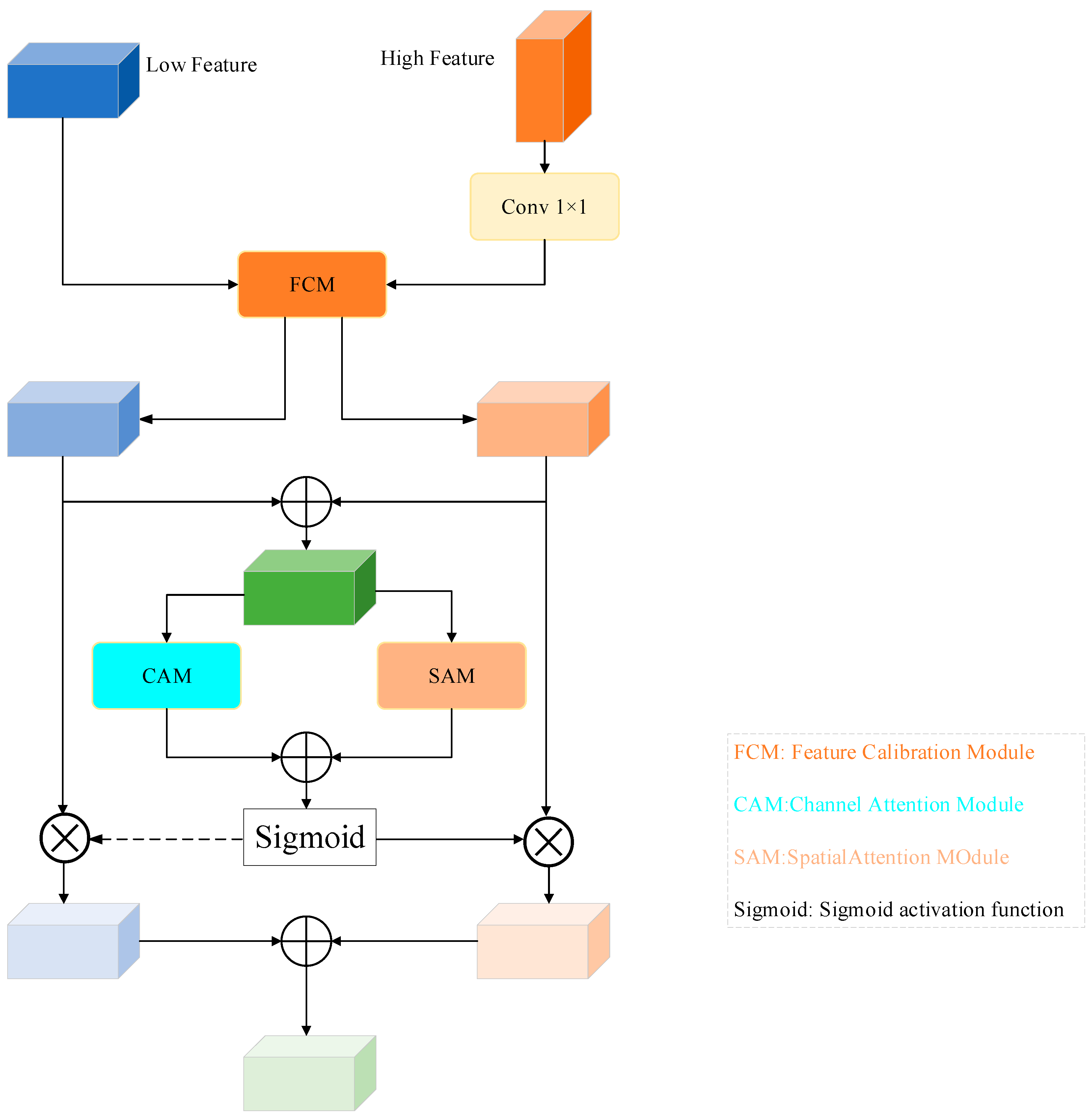
2.5. Cross-Scale Multi-Level Feature Fusion Module

After five stages of the backbone network, the model extracts multi-layer features with global contextual information. Similar to FPN-like networks, low-level features contain coarse-grained information with a relatively high resolution; high-level features contain fine-grained information, but with a relatively low resolution. While in the decoding stage, traditional UNet models often employ the simple upsampling of high-level features, to match the spatial scale of low-level features, followed by concatenation. However, the simple upsampling only makes the feature size of the high and low layers consistent; it cannot eliminate the corresponding error between the high- and low-layer feature pixels. Consequently, this approach falls short in resolving spatial misalignment between features, resulting in substantial information loss, and adversely affecting the overall performance of the model [49]. In addition, this operation easily generates semantic gaps, which lead to the occurrence of situations such as the omission of small water bodies, and the misclassification of shadow targets. To solve the above problems, we design a cross-scale, multi-source feature fusion module, to replace the decoder block in UNet.

As shown in Figure 3, for two feature maps with different scales and channel numbers as inputs to the module, we assume that the high-level input features are X_h, and the low-level input features are X_l, whose sizes are 2C × H × W and C × 2H × 2W, respectively, where C represents the number of channels of the feature map, and H and W are the height and width. To ensure that the high-level features include the same channels as the low-level features, a 1 × 1 convolution operation is initially applied to X_h. Then, inspired by Li et at. [49] and Huang et al. [50], we put the high-level and low-level features into a designed feature calibration module, so that we could obtain the spatially dimensional aligned high- and low-level features X_h2 and X_l1 (both of the sizes C × 2H × 2W). Subsequently, the high- and low-level features are summed, to obtain the fusion feature X_f. For the fusion feature, we perform the attention mechanism along the spatial and channel dimensions, respectively, to obtain the spatial weight M_s and the channel weight M_c, and then we sum the outputs of the two to obtain the output X_f1, and then we obtain the weights via the sigmoid activation function. The output variables X_h3 and X_l2 are generated via multiplying the weight coefficients s and (1 − s) with X_h2 and X_l1, respectively, which are then summed to obtain the final feature map X_out. The above process can be expressed as a series of equations:

$${\mathrm{X}}_{\mathrm{l}1},{\mathrm{X}}_{\mathrm{h}2}=\mathrm{F}\mathrm{A}\mathrm{M}({\mathrm{X}}_{\mathrm{l}},{\mathrm{f}}^{1\times 1}({\mathrm{X}}_{\mathrm{h}}\left)\right)$$

(7)

$${\mathrm{X}}_{\mathrm{f}}={\mathrm{X}}_{\mathrm{l}1}+{\mathrm{X}}_{\mathrm{h}2}$$

(8)

$${\mathrm{X}}_{\mathrm{f}1}=\mathrm{C}\mathrm{A}\mathrm{M}\left({\mathrm{X}}_{\mathrm{f}}\right)+\mathrm{S}\mathrm{A}\mathrm{M}\left({\mathrm{X}}_{\mathrm{f}}\right)$$

(9)

$$\mathrm{s}=\mathrm{s}\mathrm{i}\mathrm{g}\mathrm{m}\mathrm{o}\mathrm{i}\mathrm{d}\left({\mathrm{X}}_{\mathrm{f}1}\right)$$

(10)

$${\mathrm{X}}_{\mathrm{o}\mathrm{u}\mathrm{t}}={\mathrm{X}}_{\mathrm{l}1}·(1-\mathrm{s})+{\mathrm{X}}_{\mathrm{h}2}·\mathrm{s}$$

(11)

where f^1×1() denotes the 1 × 1 convolution layer, while the abbreviations FCM, CAM, and SAM, respectively, denote the feature calibration module, channel attention module, and spatial attention module. For further details regarding these modules, please refer to Section 2.5.1, Section 2.5.2 and Section 2.5.3 of this paper.

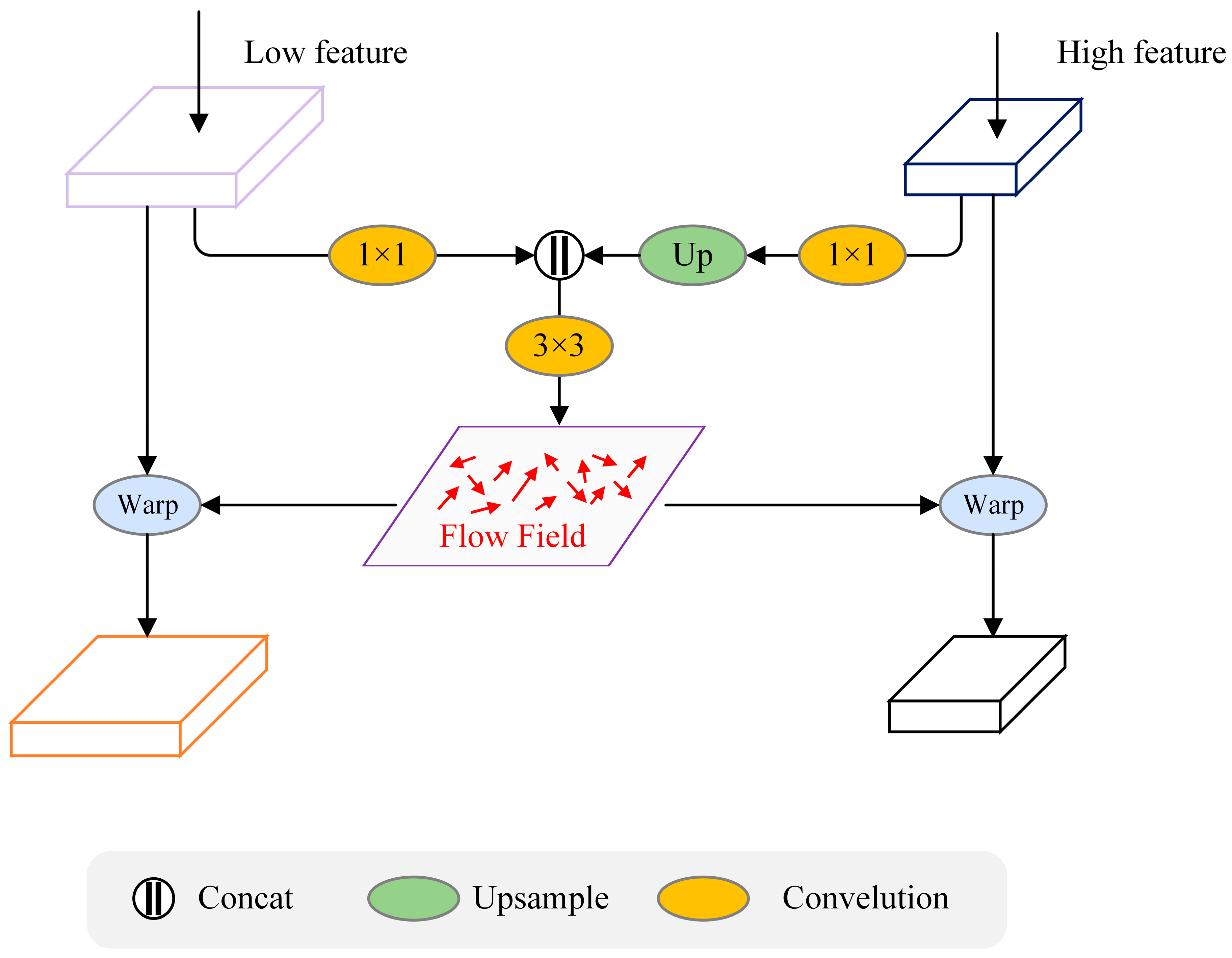
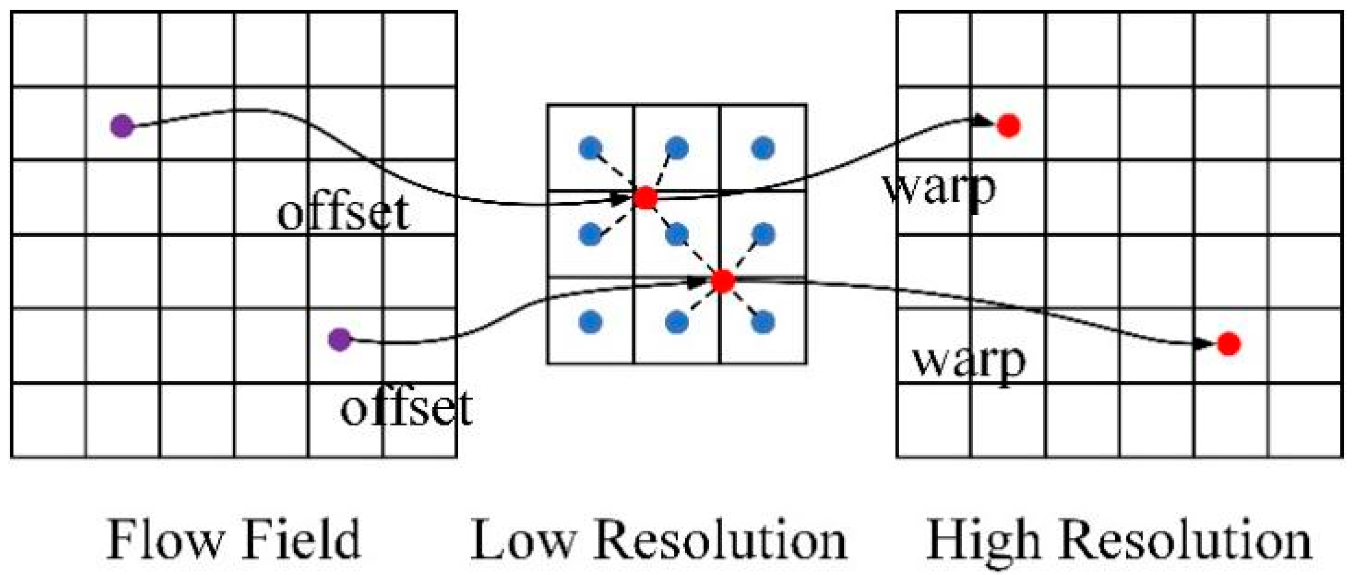
2.5.1. Feature Calibration Module

In semantic segmentation tasks, low-level features contain abundant spatial information, but are limited in terms of semantic information, while high-level features exhibit the opposite characteristics, being abundant in semantic information, but lacking in contextual and spatial details. In the decoder stage, the challenge lies in how to effectively fuse multi-scale hierarchical semantic features, to obtain rich spatial and semantic information for pixel classification. Previous works have explored this issue [24,26,51,52]. However, many of these works often overlook a crucial problem, which is the feature misalignment issue across different scales.

The problem of feature misalignment refers to the misalignment or mismatch between features caused by differences in the receptive field sizes and resolutions at different scales. This may lead to issues such as blurry boundaries and misclassification of objects in the segmentation results. The main cause of feature misalignment across multiple scales lies in the up-sampling and down-sampling operations used in the models. During scale transformations, the up-sampling and down-sampling operations employed may introduce misalignment in feature maps. For example, the interpolation method used during up-sampling may introduce positional offsets, while down-sampling may result in a loss of information and blurring effects.

To address the issue of the semantic and spatial misalignment of features on different scales, this study proposes a feature calibration module (illustrated in Figure 4). Specifically, the high-level and low-level features are first passed through individual 1 × 1 convolutional layers to adjust their dimensions, followed by up-sampling of the high-level features to align with the low-level features. Subsequently, the concatenated feature maps are processed by a 3 × 3 convolutional layer, to reduce the number of channels to four, which represent the offset maps of the high-level and low-level features in the x and y directions, as shown in Equation (12).

$${\mathsf{\Delta }}_{\mathrm{l}},{\mathsf{\Delta }}_{\mathrm{h}}={\mathrm{f}}^{3\times 3}\left(\mathrm{cat}\left({\mathrm{f}}^{1\times 1}\left({\mathrm{F}}_{\mathrm{l}}\right),{\mathrm{U}\mathrm{p}(\mathrm{f}}^{1\times 1}\left({\mathrm{F}}_{\mathrm{h}}\right))\right)\right)$$

(12)

where cat(·) represents the concatenation operation, and f^3×3(·) is the 3 × 3 convolutional layer, f^1×1(·) is the 1 × 1 convolutional layer, Up(·) denotes the up-sampling operation, and ${\mathsf{\Delta }}_{\mathrm{l}},{\mathsf{\Delta }}_{\mathrm{h}}$ represent the offset map (size H × W × 2) of the low- and high-level features.

After obtaining the offset map between the high- and low-level feature maps, we then perform a warp operation (as shown in Figure 5) on the semantic flow field of the two features, which is described in Equation (13):

$$\begin{array}{cc}{\mathrm{W}\mathrm{a}\mathrm{r}\mathrm{p}}_{\mathrm{h}\mathrm{w}}^{\mathrm{c}}=& {\displaystyle \sum _{{\mathrm{h}}^{\prime }=1}^{\mathrm{H}}} {\displaystyle \sum _{{\mathrm{w}}^{\prime }=1}^{\mathrm{W}}} {\mathrm{F}}_{{\mathrm{h}}^{\prime }{\mathrm{w}}^{\prime }}^{\mathrm{c}}\cdot \max \left(0,1-\left|\mathrm{h}+{\mathsf{\Delta }}_{\mathrm{y}}-{\mathrm{h}}^{\prime }\right|\right)\\ & \cdot \max \left(0,1-\left|\mathrm{w}+{\mathsf{\Delta }}_{\mathrm{x}}-{\mathrm{w}}^{\prime }\right|\right)\end{array}$$

(13)

where ${\mathrm{F}}_{{\mathrm{h}}_{\prime }{\mathrm{w}}_{\prime }}^{\mathrm{c}}$ is the value of the position of the original feature at the spatial level (w′, h′, c), and h, w are the height and width of the output feature map (e.g., for high-level features, h = 2 × h′, and for low-level features, h = h′). ${\mathsf{\Delta }}_{\mathrm{y}}$, ${\mathsf{\Delta }}_{\mathrm{x}}$ are the offset of the offset map obtained from the feature map in Equation (12) on the y, x axes, i.e., on the height and width.

Finally, two feature maps are obtained after calibration, with consistent height and width dimensions for both (i.e., generating the feature maps with a size of H × W × C for both).

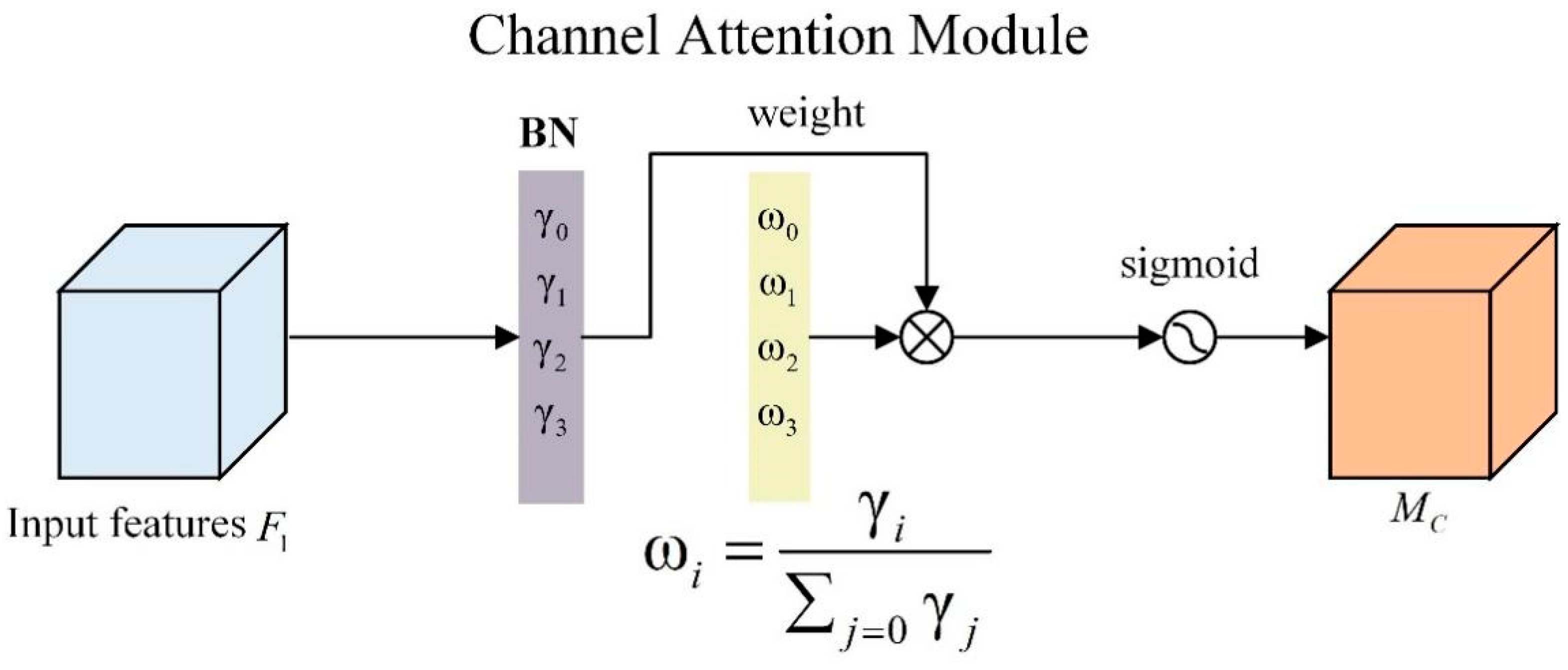
2.5.2. Channel Attention Module

Inspired by the human visual system, attention mechanisms [35] have been introduced into neural networks, to learn more relevant features. In neural networks, attention mechanisms calculate weights for each feature map in a layer, allowing the model to capture critical information more effectively. Building on the work of Liu et al., a channel attention sub-module was designed (as shown in Figure 6) to model the interdependencies between channels in the fused features. To determine the variance between channels, and infer their relative importance, a scaling factor γ was introduced into the calculation of batch normalization (BN) [53], as shown in Equation (14).

$${\mathrm{B}}_{\mathrm{out}}=\mathrm{B}\mathrm{N}\left({\mathrm{B}}_{\mathrm{in}}\right)=\mathsf{\gamma }\frac{{\mathrm{B}}_{\mathrm{in}}-{\mathsf{\mu }}_{\mathcal{B}}}{\sqrt{{\mathsf{\sigma }}_{\mathcal{B}}^2+\mathsf{ϵ}}}+\mathsf{\beta }$$

(14)

In Equation (14), μ_B and σ_B, respectively, represent the mean and standard deviation of batch B, while β denotes the bias term. The channel attention module weights, denoted as Mc, can be obtained by reversing Equation (14) using Equation (15), where γ is the scaling factor for each channel, and $\mathrm{W}\mathsf{\gamma }=\frac{{\mathsf{\gamma }}_{\mathrm{i}}}{{\sum }_{\mathrm{j}=0}{\mathsf{\gamma }}_{\mathrm{j}}}$ represents the proportion of the scaling factor for each channel among all the channels. A higher value indicates that the corresponding channel requires more attention, while a lower value suggests that the model should assign less attention to that channel.

$${\mathrm{M}}_{\mathrm{c}}=\mathrm{s}\mathrm{i}\mathrm{g}\mathrm{m}\mathrm{o}\mathrm{i}\mathrm{d}\left({\mathrm{W}}_{\mathsf{\gamma }}\left(\mathrm{B}\mathrm{N}\left({\mathrm{F}}_1\right)\right)\right)$$

(15)

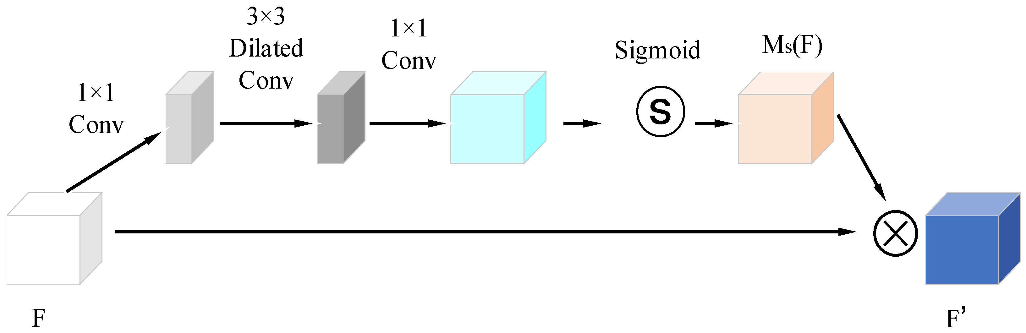
2.5.3. Spatial Attention Module

For the spatial attention module, as shown in Figure 7, we directly pass the feature map through three convolutions, followed by BN and ReLU after each convolution, and the first and last of the three convolutions are 1 × 1 convolutions for channel transformation, similar to the structure in the bottleneck. In the middle is a 3 × 3 dilation convolution, which is used to enlarge the receptive field without increasing the computational overhead. The introduction of dilated convolution and the ability to obtain more context information are of great help in providing spatial modeling. Finally, the spatial weight Ms is obtained through the sigmoid function, as shown in Formula (16).

$$\mathrm{M}\mathrm{s}\left(\mathrm{F}\right)=\mathrm{s}\mathrm{i}\mathrm{g}\mathrm{m}\mathrm{o}\mathrm{i}\mathrm{d}\left({\mathrm{f}}_2^{1\times 1}\left({\mathrm{f}}_1^{3\times 3}\right({\mathrm{f}}_0^{1\times 1}\left(\mathrm{F}\right))\right))$$

(16)

where f^3×3(·) denotes a 3 × 3 two-dimensional dilated convolution, and f^1×1(·) denotes a 1 × 1 two-dimensional convolution.

2.6. Loss Function

Cross-entropy (CE) loss and Dice loss are commonly utilized as the predominant loss function in the semantic segmentation of remote sensing images. However, these loss functions and their variants are based on region similarity, and may lead to a poor performance when dealing with imbalanced classes, as well as small objects and edge details in images. In the task of land–water segmentation, there are often many small segmentation targets in the image, such as lakes, ships, islands, buildings, and clouds. Moreover, the water–land boundary in the image is often jagged and difficult to distinguish. The use of only the Dice loss or CE loss is insufficient to address these issues.

Therefore, in this study, we incorporated the boundary loss function [54] to address the problem of edge detail handling and small object recognition in water–land semantic segmentation. The formula for computing the boundary loss is as follows:

$${\mathrm{L}}_{\mathrm{B}}=\frac{1}{\mathrm{N}}\sum _{\mathrm{i}=1}^{\mathrm{N}}\mathrm{d}\left(\mathcal{B}\left({\mathrm{y}}_{\mathrm{i}}\right),\mathcal{B}\left(\widehat{{\mathrm{y}}_{\mathrm{i}}}\right)\right)$$

(17)

where L_B denotes the boundary loss function,${\mathrm{y}}_{\mathrm{i}}$ is the ground truth label of pixel i, and $\widehat{{\mathrm{y}}_{\mathrm{i}}}$ is the predicted label of pixel i by the model. The distance function d measures the dissimilarity between two boundaries, with N representing the whole number of pixels. To address the challenges of small object recognition and edge detail handling in land–water semantic segmentation, we propose a hybrid loss function L that integrates the boundary loss function with the CE loss. Specifically, the proposed loss function L is defined as follows:

$$\mathrm{L}=\mathrm{p}·{\mathrm{L}}_{\mathrm{c}\mathrm{e}}+(1-\mathrm{p})·{\mathrm{L}}_{\mathrm{B}}$$

(18)

L_ce represents the CE loss function, and p is a weighting coefficient. Through experiments, we set p to 0.8 in this study.

3. Results

3.1. Study Area and Dataset

For this study, the Chinese coastline on the Yellow Sea was chosen as the designated study area. The image data utilized in this study were acquired from the China Center for Resources Satellite Data and Application (CCRSDA; http://www.cresda.cn, accessed on 15 April 2023). Specifically, we acquired three remote sensing images from Gaofen-6 (GF-6), captured in February 2023, with a spatial resolution of 16 m, and eight spectral bands. All the GF-6 images utilized in this study were of the Class 1A product type, characterized by a high quality and an absence of cloud cover, and provided complete coverage of the entire Yellow Sea area (see Figure 8 for further details). A detailed summary of the GF-6 images is presented in

Table 1. GF6/WFV data.

Project	GF6/WFV Data
Wavelength range/um	B1(Blue): 0.45~0.52
	B2(Green): 0.52~0.59
	B3(Red): 0.63~0.69
	B4(NIR): 0.76~0.90
	B5(SWIR1): 0.69~0.73
	B6(SWIR2): 0.73~0.77
	B7(Purple): 0.40~0.45
	B8(Yellow): 0.59~0.63
Spatial resolution/m	16
Width/km	864.2

. Subsequently, we preprocessed the original image with radiometric calibration and atmospheric correction and, ultimately, generated remote sensing images suitable for further research purposes.

In the image of the study area, the part of the sea–land boundary to be used to construct the GF dataset was selected, and sea–land segmentation was carried out. Initially, due to the excessive width of the original GF6 WFV images, and the presence of overlapping regions between the three images, we cropped these three images, while preserving the Yellow Coast as fully as possible, to reduce the difficulty of the task. Please refer to Figure 8 for specific details. Then, the clipped image was divided into two categories: ocean and land. To improve the efficiency of the training, we selected only those cropped images that contained both ocean and land, and obtained 2100 images and 2100 labels, all of which were 512 pixels × 512 pixels in size.

In cases where the network model requires an insufficient number of training samples, data augmentation becomes a crucial step in enhancing the network’s invariance and robustness. In order to increase the data volume of the experimental dataset, five data expansion methods, such as horizontal flip, vertical flip, diagonal mirror, local cropping and magnification, and image sharpening, are used to increase the image quantity of the dataset. Finally, the GF dataset we constructed contained 12,600 images, which were subsequently partitioned into training, validation, and test sets, in a random 7:2:1 ratio.

3.2. Experimental Details and Evaluation Metrics

All experiments were performed on a workstation running Windows 10 with an NVIDIA GeForce RTX 3090 graphics card, and using the deep learning framework Pytorch (2017). All models were trained with an initial learning rate of 0.001, and AdamW [48], with a momentum term of 0.9 and a weight decay of 0.01, was selected as the optimizer to optimize the network model. Additionally, to speed up the training, we set the batch size to 16, and the epoch number to 100. The poly method is used to dynamically adjust the learning rate. The formula is expressed as follows:

$${\mathrm{l}}_{\mathrm{i}}={\mathrm{l}}_{\mathrm{b}\mathrm{a}\mathrm{s}\mathrm{e}}\times {\left(1-\frac{{\mathrm{epoch}}_{\mathrm{i}}}{{\mathrm{epoch}}_{\mathrm{m}\mathrm{a}\mathrm{x}}}\right)}^{0.9}$$

(19)

where l_i is the current learning rate, l_base is the base learning rate set to 0.001, epoch_i is the current number of iterations, and epoch_max is the maximum epoch set to 100.

In this paper, three metrics normally utilized in semantic segmentation are used to verify the effectiveness of the model, namely the pixel accuracy (PA), mean intersection over union (MIoU), and F1-score. Based on the associated confusion matrix, the PA, MIoU, and F1 are calculated as

$$\mathrm{P}\mathrm{A}=\frac{{\displaystyle {\sum }_{\mathrm{k}=1}^{\mathrm{K}}}{\mathrm{T}\mathrm{P}}_{\mathrm{k}}}{{\displaystyle {\sum }_{\mathrm{k}=1}^{\mathrm{K}}}({\mathrm{T}\mathrm{P}}_{\mathrm{k}}+{\mathrm{F}\mathrm{P}}_{\mathrm{k}}+{\mathrm{T}\mathrm{N}}_{\mathrm{k}}+{\mathrm{F}\mathrm{N}}_{\mathrm{k}})}$$

(20)

$$\mathrm{M}\mathrm{I}\mathrm{o}\mathrm{U}=\frac{1}{\mathrm{K}}\frac{{\displaystyle {\sum }_{\mathrm{K}=1}^{\mathrm{K}}}{\mathrm{T}\mathrm{P}}_{\mathrm{k}}}{({\mathrm{T}\mathrm{P}}_{\mathrm{k}}+{\mathrm{F}\mathrm{P}}_{\mathrm{k}}+{\mathrm{F}\mathrm{N}}_{\mathrm{k}})}$$

(21)

$$\mathrm{F}1=2\times \frac{{\mathrm{p}\mathrm{r}\mathrm{e}\mathrm{c}\mathrm{i}\mathrm{s}\mathrm{i}\mathrm{o}\mathrm{n}}_{\mathrm{k}}\times {\mathrm{r}\mathrm{e}\mathrm{c}\mathrm{a}\mathrm{l}\mathrm{l}}_{\mathrm{k}}}{{\mathrm{p}\mathrm{r}\mathrm{e}\mathrm{c}\mathrm{i}\mathrm{s}\mathrm{i}\mathrm{o}\mathrm{n}}_{\mathrm{k}}+{\mathrm{r}\mathrm{e}\mathrm{c}\mathrm{a}\mathrm{l}\mathrm{l}}_{\mathrm{k}}}$$

(22)

where TP_k, FP_k, TN_k, and FN_k represent the true positive, false positive, true negative, and false negative values for the kth class, respectively. In addition, precision_k = $\frac{{\mathrm{T}\mathrm{P}}_{\mathrm{k}}}{{\mathrm{T}\mathrm{P}}_{\mathrm{k}}+{\mathrm{F}\mathrm{P}}_{\mathrm{k}}}$ and recall_k = $\frac{{\mathrm{T}\mathrm{P}}_{\mathrm{k}}}{{\mathrm{T}\mathrm{P}}_{\mathrm{k}}+{\mathrm{F}\mathrm{N}}_{\mathrm{k}}}$ are the precision and recall rates for the k classes, respectively.

3.3. Performance Comparison of Different Band Combinations

The GF6 image is a typical multispectral remote sensing image. Compared with the traditional RGB image, multispectral images contain a significantly greater amount of information, due to their higher number of bands (the GF6 has eight bands). This paper, firstly, discusses the effectiveness of different band combinations in sea–land segmentation. According to Yu et al. [55] and Mou et al. [56], we selected ten common three-band and all-band combinations, and compared their performance differences on sea–land semantic segmentation. Details of the comparison experiment of band combination are presented in

Table 2. Comparison of results of different band combinations on the GF dataset.

Band Combination	PA (%)	MIoU (%)	F1 (%)
B1 + B2 + B3	96.52	91.12	95.30
B1 + B4 + B5	96.81	92.23	95.36
B2 + B3 + B4	96.95	92.64	95.58
B2 + B3 + B5	96.21	91.81	94.88
B3 + B4 + B5	96.99	92.78	95.67
B3 + B4 + B8	96.64	92.07	95.27
B3 + B5 + B7	95.89	89.56	94.32
B4 + B5 + B6	96.69	92.19	95.33
B4 + B6 + B7	96.31	91.28	94.82
B5 + B6 + B7	96.88	92.36	95.43
All-bands	97.52	93.53	96.63

.

As seen in Table 2, bands 3, 4, and 5 (Red, Nir, and Swir-1) outperformed the other nine bands in the sea–land segmentation task. However, the effect of the all-band combination is better than that of all the three-band combinations. This shows that the eight different bands can contain more spatial and spectral information, and that the complementary information is more advantageous in the task of sea–land semantic segmentation.

3.4. Ablation Study

3.4.1. Performance of Feature Interaction Module

To assess the performance of the FIM, this article conducted ablation research to validate the effectiveness of the module design. We divided the experiment into three scenarios: (1) only using CNN branches as encoders; (2) using only transformer branches as encoders; (3) the method proposed in this article, to use dual branches and, simultaneously, use FIM as encoders. For the decoder part, we uniformly used the designed CMFFM. The outcomes of the experiment are presented in

Table 3. Results of the module ablation experiments. The best results are in bold.

Method	Encoder	PA (%)	MIoU (%)
TCU-Net	CNN	96.02	92.01
	Transformer	95.89	91.95
	CNN + Transformer + FIM	97.52	93.53

.

Table 3 reveals that the segmentation accuracy using only the Transformer branch as the encoder is the worst, with an MIoU of 91.95% and a PA of 95.89%, while the segmentation accuracy using only the CNN branch is not high, with an MIoU of 92.01% and a PA of 96.02. There is a certain gap between the segmentation accuracy of the two branches and the FIM as the encoder. This shows that simply using a CNN or Transformer branch as the encoder has certain defects in feature extraction, and cannot integrate image spatial information, semantic information, and global context information well. After the introduction of the FIM as the information exchange bridge between the two branches, the missing local and global information perception ability between the two branches is enhanced, the information exchange and complementary function are perfectly realized, and the feature extraction ability of the whole model is greatly enhanced.

3.4.2. Performance of Cross-Scale, Multi-Level Feature Fusion Module

In order to evaluate the performance of the cross-scale, multi-level feature fusion module, we verified the effect of the module for small targets and edge extraction in images. In this paper, we use TCU-Net as a baseline to perform ablation experiments on the Yellow Sea sea–land semantic segmentation dataset.

The results of the experiment are shown in

Table 4. Results of the module ablation experiments.

Method	Decoder	PA (%)	MIoU (%)	F1 (%)	Params (M)
TCU-Net	UNet	96.91	93.01	96.02	2.4 M
	CSMFF	97.52	93.53	96.63	1.72 M

. Through comparing the feature fusion strategies, we find that the simple up-sampling and jump join, as in the original UNet, can not fully fuse semantic features of different scales and levels. Through using the proposed CSMFF module, the PA, MIoU, and F1-score are improved by 0.51%, 0.31%, and 0.36%, respectively, on the test set. Simultaneously, the number of parameters of the CSMFF module designed in this paper is reduced by 0.68 M, compared with the jump connection of the original UNet, which further upgrades the efficiency of the model in processing images.

The visualization results from the experiment are shown in Figure 9. In order to show the difference in the prediction results between the two decoders more directly, blue boxes are used to highlight the positions where the model shows differences in the prediction image. It is evident that the TCUNet using the decoder of the original UNet performs poorly on the sea–land boundary and the small water body when predicting the picture, because the shallow feature and the deep feature are spliced only using up-sampling and the jump connection, and semantic gaps are easily generated, resulting in the situation whereby the small water body is missed, and the shadow target is misclassified. Using the CSMFF module designed in this paper as a decoder can effectively improve the detection of small objects and the definition of boundaries in the land–sea segmentation task, so that the classification results of the model are more accurate.

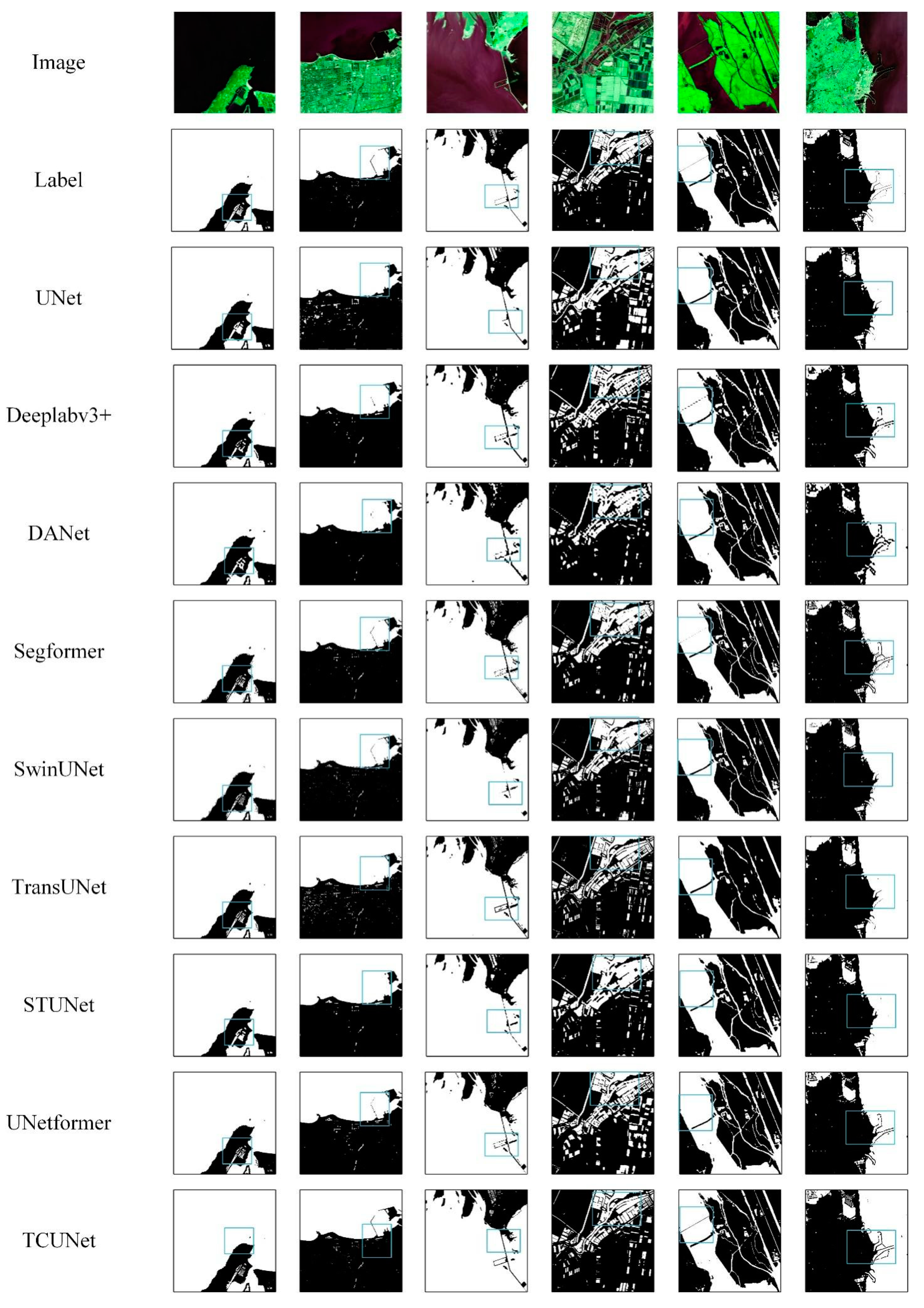
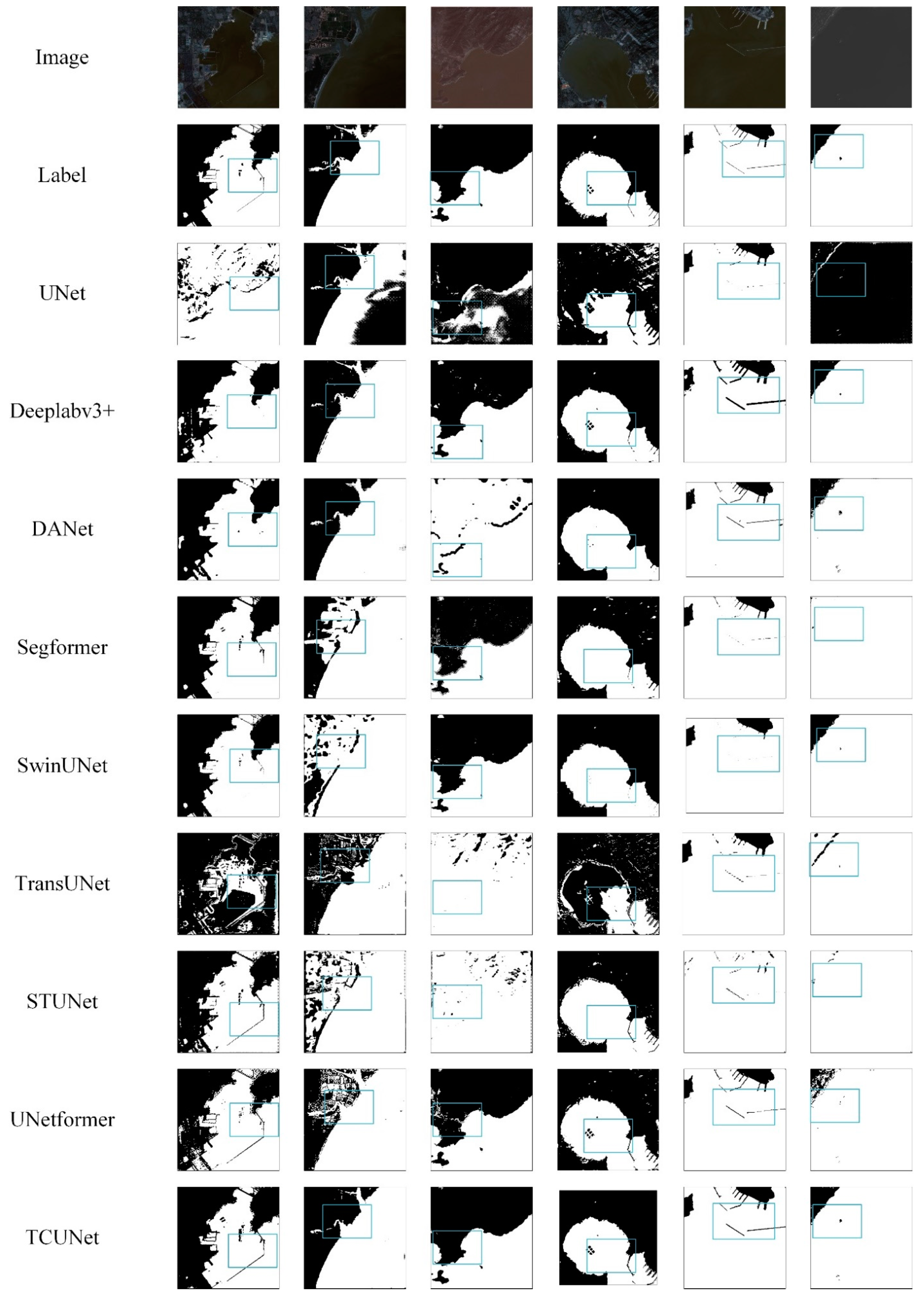
3.5. Contrast Experiment

To more accurately evaluate the performance of the model proposed in this paper, we compare our model with some excellent models commonly found in the field of semantic segmentation, including UNet, Deeplabv3+, DANet [51], Segformer, SwinUNet [57], TransUNet, ST-UNet, and UNetformer [58]. The first three methods are CNN networks, Segformer and SwinUNet are pure vision sensor methods, and TransUNet, ST-UNet, and UNetformer are hybrid models that combine CNNs with sensors. The TransUNet encoder adopts the serial form of standard ViT and ResNet, and the decoder is the same as UNet; ST-UNet improves the encoder part on the basis of TransUNet, using a dual-encoder structure with a Swin transformer and CNN in parallel, while UNetformer uses ResNet18 as the encoder, and develops an efficient global–local attention mechanism to construct transformer blocks in the decoder, as the decoder. In addition, the backbone of Deeplabv3+ and DANet is ResNet50, that of Segformer is MiT-B1, and the backbones of other models are set by the original authors. In addition, according to the experiment in 3.3, for UNetformer, which only accepts three-band image input (its backbone is the officially packaged ResNet18), we chose the band combination of bands 2, 3, and 5 as its input data, while the other models used the full-band combination (8 bands) as their input data. To ensure the fairness of the experiment, no models were pre-trained. The experiments were carried out under the same conditions, and the specific implementation details are shown in Section 3.2. of this paper. The quantitative analysis results of the GF dataset are shown in

Table 5. Comparison of all the methods in metrics. Training Time represents the time spent by the model in processing the training and validation sets during training; Inference Time represents the time spent processing the test set when the model makes predictions.

Method	Backbone	PA (%)	MIoU (%)	F1 (%)	Params (M)	FLOPs (GMac)	Training Time (s)	Inference Time (s)
UNet [24]	-	96.95	92.15	95.96	31.04	218.9	695	86.28
Deeplabv3+ [28]	ResNet50	96.87	91.98	95.77	40.36	70.22	385	77.28
DANet [51]	ResNet50	96.68	91.52	95.52	49.61	205.37	680	85.44
Segformer [40]	MiT-B1	97.16	92.71	96.18	13.69	13.49	375	78.48
SwinUNet [57]	Swin-Tiny	96.88	91.95	95.92	27.18	26.56	505	84.36
TransUNet [41]	ViT-R50	97.07	92.41	96.03	100.44	25.5	810	106.26
ST-UNet [44]	-	97.23	92.99	96.34	160.97	95.41	915	135.54
UNetformer [58]	ResNet18	97.15	92.67	96.15	11.72	11.73	235	73.44
TCUNet	-	97.52	93.53	96.63	1.72	3.24	445	87.78

, and the best results of each evaluation index are highlighted in bold.

The results show that the TCUNet proposed in this paper is superior to the other eight models in its PA, MioU, and F1-score. Overall, the combination of CNN and Transformer worked slightly better than the visual Transformer method, and the CNN-based method showed the worst classification accuracy, but there was no significant difference between the nine methods. This shows that the CNN-based model has some limitations in describing global dependencies. In the CNN method, the effect of UNet is the best, that of Deeplabv3 + is the second best, and the effect of DANet is the worst. This may be due to the fact that UNet adopts a feature pyramid-like structure in the decoder, which fuses the five layers of semantic features extracted by the backbone network through jumping links; it can be applied to the sea–land segmentation of high-level semantic information and detail information. However, Deeplabv3 + uses hole convolution and an ASPP module to integrate multi-layer semantic features, which is too simple, and not good for the fine segmentation of object edges and details. DANet’s encoder only uses the high-level semantic features of the backbone network for classification, meaning that it can not make full use of the shallow semantic features, and the classification effect is the worst. Among the Transformer models, TCUNet is the best, ST-UNet is the second, Segformer and UNetformer have the same classification accuracy, slightly better than TransUNet, and SwinUNet is the worst.

Figure 10 shows the segmentation results for all the methods in the six test images. Looking at Figure 10, we can see that TCUNet performed better on segmentation than the other eight models, especially in the blue-rectangular-box-labeled area. As can be seen from these test charts, the proposed method shows the best segmentation effect compared with the other models. Faced with complex types of shorelines (farmed ponds, ports, small rivers), our networks can still clearly delineate boundaries. At the same time, in the edge details and small target recognition, compared with other methods, our network segmentation is better. This shows that our network model can solve the problems of missed detection and misclassification in low contrast areas and small water bodies with a complex background, and effectively improve the problems of pixel classification, small target extraction, and boundary blur, meaning that the effect of classification is more accurate.

In order to evaluate the segmentation efficiency of all the models, we also list the number of parameters, the computational complexity, and the time spent on training and reasoning of each model in Table 5, where “M” represents one million parameters, and “GMac” stands for the billion times a model performs a floating-point multiplication and addition operation in the course of a single forward propagation. The model proposed in this paper is only 1.72 M and 3.24 GMac, far lower than the other eight models. This is because the two-branch structure used in this paper greatly enhances the ability of the model to extract semantic features, so we set the number of channels in the first stage of the model to 16 (that is, greatly reducing the width of the network) without affecting the performance of the network. In terms of the training and prediction efficiency, the training time of TCUNet is 89 s per epoch, and the inference time is 14.63 s, which ranks medium among all models. The lightweight model UNetformer runs much faster than other networks. This may be because the hybrid structure of the CNN and transformer in TCUNet slows down the running efficiency of the model, and there are many LN and GELU [59] functions in FIM, which are far less optimized via the graphics card than the convolution and ReLU operations of a traditional CNN. This will cause TCUNet to be slower when processing images. Although the above two issues may limit the application of TCUNet in some scenarios (such as on small mobile devices), TCUNet is still valuable in exploring the role of the transformer and CNN combination in sea–land semantic segmentation in remote sensing images.

4. Discussion

4.1. Comparison of Model Effects on Different Satellite Sensor Images

Various satellite sensors can collect different remote sensing images in the same geographical area. In order to verify the adaptability of our model to different satellite images at different time periods, we selected a Landsat 8/OLI remote sensing image of the Yellow Sea region in October 2019, to verify the portability of the model. The OLI sensor has a total of 9 bands, with bands 1–7 and 9 having a spatial resolution of 30 m, and band 8 having a panchromatic resolution of 15 m. The detailed information is listed in

Table 6. Landsat8/OLI data.

Project	Landsat 8/OLI
Wavelength range/um	B1(Coastal aerosol): 0.43~0.55
	B2(Blue): 0.45–0.51
	B3(Green): 0.53–0.59
	B4(Red):0.64–0.67
	B5(NIR): 0.85–0.88
	B6(SWIR1): 1.57–1.65
	B7(SWIR2): 2.11–2.29
	B8(PAN): 0.50–0.68
Spatial resolution/m	15
Width/km	185

. In order to ensure that the number of bands in the data is consistent with GF6/WFV, this article will perform image fusion on the first seven bands and panchromatic bands after some preprocessing steps, such as radiation calibration and FLAASH atmospheric correction. Finally, an 8-band image, with a resolution of 15 m, was obtained. As with the GF6 image, we selected part of the sea–land boundary, to construct a Landsat dataset for validation experiments. After cropping and labeling, 112 images and labels were obtained; all images had a size of 512 pixels × 512 pixels. Subsequently, we used five data expansion methods, including horizontal flipping, vertical flipping, diagonal mirroring, local cropping, and zooming in, and image sharpening, to increase the number of images in the dataset, resulting in 672 images and labels.

Without training and parameter adjustments, we directly predicted the 672 images using the model weights trained in 3.5, exploring the land and sea segmentation effects of each model on remote sensing images of the same area from different satellites and at different time points. The experimental results are shown in

Table 7. The results of all methods on the Landsat datasets.

Method	PA (%)	MIoU (%)	F1 (%)
UNet	64.63	41.55	61.25
Deeplabv3+	91.75	83.82	91.13
DANet	88.23	76.84	86.72
Segformer	80.88	67.83	80.63
SwinUNet	81.04	68.03	80.96
TransUNet	75.10	60.60	74.92
ST-UNet	84.82	73.41	84.65
UNetformer	90.17	80.20	88.89
TCUNet	95.46	90.84	95.19

. The indicators of TCUNet in the PA, F1-Score, and MIoU are 95.46%, 95.19%, and 90.84%, respectively, which are much higher than those of the other nine models.

In addition, for the segmentation results of Landsat images, as shown in Figure 11, in order to visually verify the segmentation effect of each method, this article uses blue boxes to highlight the positions where the model shows differences in the predicted image. It can be clearly seen that without pre-training, Deeplabv3+, UNeformer, and DANet perform well. However, it can be seen from the graph that these models cannot perform the precise segmentation of water and land, and there is a phenomenon of misclassification and missing segmentation for small targets, such as ships, islands, and ponds. However, the segmentation results of Segformer, TransUNet, and SwinUNet are not satisfactory, and cannot accurately complete land and sea segmentation. They can only roughly distinguish between water and land. U-Net cannot perform land and sea segmentation in Landsat 8 images. This indicates that U-Net struggles to extract water bodies from different remote sensing images across sensors, despite its excellent performance in medical images. The TCUNet method proposed in this article can extract the coastline at different times, across sensors. The accuracy of the extraction results meets the extraction requirements.

4.2. Performance under Different Parameter Settings

In this paper, we continue to explore the sea–land segmentation task, by setting different parameters, to test the segmentation performance of the model. The experimental results are shown in

Table 8. Performance under different parameter settings. E represents the dimension of the first stage of the Transformer branch. C represents the number of channels in the first layer of the CNN branch, and D represents the number of Conv blocks and Transformer blocks in stages 2–5.

E	C	D	PA (%)	Params
16	16	[2,2,2,2]	96.92	1.04 M
		[3,4,6,3]	97.52	1.72 M
46	32	[2,2,2,2]	97.06	7.07 M
		[3,4,6,3]	97.46	8.50 M
92	64	[2,2,2,2]	97.42	20.43 M
		[3,4,6,3]	97.56	33.51 M

.

As can be seen from Table 3, increasing the number of dual-branch channels in the first stage (stages 2–5 have twice as many channels as the previous stage, as described in Section 2.2, i.e., they deepen the width of the network) does not significantly improve the segmentation performance of the model, but the parameters and complexity of the model have increased by tens of times. On the contrary, through keeping the number of model channels constant, and increasing the number of double-branch encoder modules in layers 2–5 (i.e., increasing the depth of the network), the segmentation precision of the model is obviously improved, and the parameters of the model did not increase significantly.

In response to the aforementioned phenomenon, we speculate that our proposed model, which combines a CNN and Transformer, exhibits a considerably enhanced ability in feature extraction compared to conventional CNN networks. Consequently, each layer of the model does not require too many channels (i.e., the width of the network does not need to be too wide) to obtain sufficient rich information. Correspondingly, increasing the number of channels in each layer of the network does not significantly improve the segmentation accuracy. However, network depth enhancement can enable the model to learn deeper feature information, and more complex representations of the image. As a result, enhancing the depth of the model is more effective in improving the accuracy of land and sea segmentation, in comparison with increasing the width of the module, while it also contributes to a reduction in the computational overheads.

Therefore, combining the network complexity and the model segmentation accuracy, we set the channel number of the first stage model to 16, and set the number of encoder blocks in layers 2–5 of the network to 3, 4, 6, and 3, respectively.

4.3. Limitations of the Model and Future Prospects

This paper presents a TCU-Net model specifically designed for the extraction of the shoreline from multispectral remote sensing images. Compared with the latest CNN and Transformer methods, the proposed model achieves a better segmentation accuracy with fewer model parameters and computational resources.

However, due to the inherent computational demands of the parallel dual-branch encoder structure and the Transformer model, despite efforts to reduce the model’s computational overhead through narrowing the network width and designing lightweight decoder structures, optimal results in terms of training and inference speed have not been achieved in this study. Future research will focus on further optimizing the model architecture, while ensuring a robust segmentation accuracy. This will involve the design of more efficient model structures and effective training strategies, aiming to alleviate training complexity and difficulty.

5. Conclusions

In order to achieve the high-precision segmentation of sea–land boundaries and coastline extraction from remote sensing images, a lightweight two-branch parallel network model combining CNN and Transformer is designed for sea–land segmentation in remote sensing images.

Specifically, in the encoding process of the algorithm, the CNN branch and the Transformer branch are used to extract the local semantic features and the global spatial features of the multi-spectral remote sensing image. At the same time, we design a feature interaction module (FIM) which is embedded between each corresponding two-branch coding block, serving as a bridge module to fuse the local features from the CNN branch and the global representation from the Transformer branch, to realize information interaction between the twobranches’ features. For the decoder part, we designed a cross-scale, multi-source feature fusion module (CMFFM) to replace the original UNet encoder module, achieving the successful integration of low-level semantic and high-level abstract features, and improving the network’s ability to capture information flows. For CMFFM, the module is first replaced via up-sampling using a feature calibration module, which can reduce the semantic differences between the “corresponding” pixels of images at different scales. At the same time, a channel attention module and spatial attention module are introduced to obtain channel and spatial attention weights, using two branches with different scales for the fused features, so that the model can capture the spatial and band information of the image, and realize the successful integration of low-level semantics and high-level abstract features. Finally, the fused multi-scale features are obtained. In this study, we generated a dataset, named the GF dataset for sealand segmentation in the Yellow Coastline region, using three GF-6 remote sensing satellite images. Subsequently, an extensive series of comprehensive experiments was conducted, to evaluate the segmentation performance and efficiency of TCUNet in comparison to other existing semantic segmentation networks on this dataset. The experimental results demonstrate that TCUNet has a better segmentation effect than other classical semantic segmentation networks, highlighting its superiority and effectiveness. Furthermore, we also discussed the application of the model on different band combinations and different remote sensing sensor images. In summary, this study provides a new method for extracting the coastline from remote sensing images accurately and effectively.

In our future research, we will continue to refine our model, collect multi-spectral satellite remote sensing images taken by different satellites, at different band settings and spatial resolutions, improve the application scope of the model and the accuracy of shoreline extraction, and then expand the research area, to achieve the extraction of shorelines in other sea areas.

References

1. Zollini, S.; Alicandro, M.; Cuevas-González, M.; Baiocchi, V.; Dominici, D.; Buscema, P.M. Shoreline extraction based on an active connection matrix (ACM) image enhancement strategy. J. Mar. Sci. Eng. 2020, 8, 9. [Google Scholar] [CrossRef]
2. Boak, E.H.; Turner, I.L. Shoreline Definition and Detection: A Review. J. Coast. Res. 2005, 21, 688–703. [Google Scholar] [CrossRef]
3. Soloy, A.; Turki, I.; Lecoq, N.; Gutiérrez Barceló, Á.D.; Costa, S.; Laignel, B.; Bazin, B.; Soufflet, Y.; Le Louargant, L.; Maquaire, O. A fully automated method for monitoring the intertidal topography using Video Monitoring Systems. Coast. Eng. 2021, 167, 103894. [Google Scholar] [CrossRef]
4. Yang, L.; Wang, X.; Zhai, J. Waterline Extraction for Artificial Coast With Vision Transformers. Front. Environ. Sci. 2022, 10, 16. [Google Scholar] [CrossRef]
5. Bengoufa, S.; Niculescu, S.; Mihoubi, M.K.; Belkessa, R.; Abbad, K. Rocky Shoreline Extraction Using a Deep Learning Model and Object-Based Image Analysis. Int. Arch. Photogramm. Remote Sens. Spat. Inf. Sci. ISPRS Arch. 2021, 43, 23–29. [Google Scholar]
6. Bengoufa, S.; Niculescu, S.; Mihoubi, M.K.; Belkessa, R.; Rami, A.; Rabehi, W.; Abbad, K. Machine Learning and Shoreline Monitoring Using Optical Satellite Images: Case Study of the Mostaganem Shoreline, Algeria. J. Appl. Remote Sens. 2021, 15, 026509. [Google Scholar] [CrossRef]
7. Liu, Z.; Chen, X.; Zhou, S.; Yu, H.; Guo, J.; Liu, Y. DUPnet: Water Body Segmentation with Dense Block and Multi-Scale Spatial Pyramid Pooling for Remote Sensing Images. Remote Sens. 2022, 14, 5567. [Google Scholar] [CrossRef]
8. Pardo-Pascual, J.E.; Almonacid-Caballer, J.; Ruiz, L.A.; Palomar-Vazquez, J. Automatic extraction of shorelines from Landsat TM and ETM+ multi-temporal images with subpixel precision. Remote Sens. Environ. 2012, 123, 1–11. [Google Scholar] [CrossRef]
9. Lecun, Y.; Bengio, Y.; Hinton, G. Deep learning. Nature 2015, 521, 436. [Google Scholar] [CrossRef]
10. McFeeters, S.K. The use of the Normalized Difference Water Index (NDWI) in the delineation of open water features. Int. J. Remote Sens. 1996, 17, 1425–1432. [Google Scholar] [CrossRef]
11. Xu, H. Modification of normalised difference water index (NDWI) to enhance open water features in remotely sensed imagery. J. Remote Sens. 2006, 27, 3025–3033. [Google Scholar] [CrossRef]
12. Yang, C.S.; Park, J.H.; Rashid, H.A. An Improved Method of Land Masking for Synthetic Aperture Radar-based Ship Detection. J. Navig. 2018, 71, 788–804. [Google Scholar] [CrossRef]
13. Kanopoulos, N.; Vasanthavada, N.; Baker, R.L. Design of an image edge detection filter using the Sobel operator. IEEE J. Solid-State Circuits 1988, 23, 358–367. [Google Scholar] [CrossRef]
14. Liu, H.; Jezek, K.C. Automated extraction of coastline from satellite imagery by integrating Canny edge detection and locally adaptive thresholding methods. Int. J. Remote Sens. 2004, 25, 937–958. [Google Scholar] [CrossRef]
15. Toure, S.; Diop, O.; Kpalma, K.; Maiga, A.S. Shoreline detection using optical remote sensing: A review. ISPRS Int. J. Geo-Inf. 2019, 8, 75. [Google Scholar] [CrossRef]
16. Wu, Y.; Liu, Z. Research progress on methods of automatic coastline extraction based on remote sensing images. J. Remote Sens. 2019, 23, 582–602. [Google Scholar] [CrossRef]
17. Breiman, L. Random forests. Mach. Learn. 2001, 45, 5–32. [Google Scholar] [CrossRef]
18. Suykens, J.A.K.; Vandewalle, J. Least Squares Support Vector Machine Classifiers. Neural Process. Lett. 1999, 9, 293–300. [Google Scholar] [CrossRef]
19. Cui, B.; Jing, W.; Huang, L.; Li, Z.; Lu, Y. SANet: A Sea–Land Segmentation Network Via Adaptive Multiscale Feature Learning. IEEE J. Sel. Top. Appl. Earth Obs. Remote Sens. 2021, 14, 116–126. [Google Scholar] [CrossRef]
20. Chen, L.C.; Papandreou, G.; Kokkinos, I.; Murphy, K.; Yuille, A.L. Semantic image segmentation with deep convolutional nets and fully connected crfs. arXiv 2014, arXiv:1412.7062. [Google Scholar]
21. Girshick, R.; Donahue, J.; Darrell, T.; Malik, J. Rich Feature Hierarchies for Accurate Object Detection and Semantic Segmentation. In Proceedings of the 2014 IEEE Conference on Computer Vision and Pattern Recognition (CVPR), Columbus, OH, USA, 23–28 June 2014; pp. 580–587. [Google Scholar]
22. Kalchbrenner, N.; Grefenstette, E.; Blunsom, P. A convolutional neural network for modelling sentences. arXiv 2014, arXiv:14042188. [Google Scholar]
23. Long, J.; Shelhamer, E.; Darrell, T. Fully Convolutional Networks for Semantic Segmentation. In Proceedings of the IEEE Conference on Computer Vision and Pattern Recognition, Boston, MA, USA, 7–12 June 2015; pp. 3431–3440. [Google Scholar]
24. Ronneberger, O.; Fischer, P.; Brox, T. U-net: Convolutional networks for biomedical image segmentation. In Proceedings of the International Conference on Medical Image Computing and Computer-Assisted Intervention, Munich, Germany, 5–9 October 2015; pp. 234–241. [Google Scholar]
25. Badrinarayanan, V.; Kendall, A.; Cipolla, R. SegNet: A Deep Convolutional Encoder-Decoder Architecture for Image Segmentation. IEEE Trans. Pattern Anal. Mach. Intell. 2015, 39, 2481–2495. [Google Scholar] [CrossRef] [PubMed]
26. Zhao, H.; Shi, J.; Qi, X.; Wang, X.; Jia, J. Pyramid Scene Parsing Network. In Proceedings of the IEEE Conference on Computer Vision and Pattern Recognition, Honolulu, HI, USA, 21–26 July 2017; pp. 2881–2890. [Google Scholar]
27. Chen, L.C.; Papandreou, G.; Kokkinos, I.; Murphy, K.; Yuille, A.L. DeepLab: Semantic Image Segmentation with Deep Convolutional Nets, Atrous Convolution, and Fully Connected CRFs. arXiv 2017, arXiv:1606.00915. [Google Scholar] [CrossRef]
28. Chen, L.C.; Zhu, Y.; Papandreou, G.; Schroff, F.; Adam, H. Encoder-Decoder with Atrous Separable Convolution for Semantic Image Segmentation. In Proceedings of the European Conference on Computer Vision (ECCV), Munich, Germany, 8–14 September 2018; pp. 801–818. [Google Scholar]
29. Sun, K.; Xiao, B.; Liu, D.; Wang, J. Deep high-resolution representation learning for human pose estimation. In Proceedings of the IEEE/CVF Conference on Computer Vision and Pattern Recognition, Long Beach, CA, USA, 15–20 June 2019; pp. 5693–5703. [Google Scholar]
30. Li, R.; Liu, W.; Yang, L.; Sun, S.; Hu, W.; Zhang, F.; Li, W. Deepunet: A deep fully convolutional network for pixel-level sea-land segmentation. IEEE J. Sel. Top Appl. Earth Obs. Remote Sens. 2018, 11, 3954–3962. [Google Scholar] [CrossRef]
31. Shamsolmoali, P.; Zareapoor, M.; Wang, R.; Zhou, H.; Yang, J. A Novel Deep Structure U-Net for Sea-Land Segmentation in Remote Sensing Images. IEEE J. Sel. Top Appl. Earth Obs. Remote Sens. 2019, 12, 3219–3232. [Google Scholar] [CrossRef]
32. Huang, G.; Liu, Z.; van der Maaten, L.; Weinberger, K. Densely Connected Convolutional Networks. In Proceedings of the IEEE Conference on Computer Vision and Pattern Recognition, Honolulu, HI, USA, 21–26 July 2017. [Google Scholar]
33. He, K.; Zhang, X.; Ren, S.; Sun, J. Deep residual learning for image recognition. In Proceedings of the IEEE Conference on Computer Vision and Pattern Recognition, Las Vegas, NV, USA, 26 June–1 July 2016; pp. 770–778. [Google Scholar]
34. He, Y.; Yao, S.; Yang, W.; Yan, H.; Zhang, L.; Wen, Z.; Zhang, Y.; Liu, T. An Extraction Method for Glacial Lakes Based on Landsat-8 Imagery Using an Improved U-Net Network. IEEE J. Sel. Top Appl. Earth Obs. Remote Sens. 2021, 14, 6544–6558. [Google Scholar] [CrossRef]
35. Vaswani, A.; Shazeer, N.; Parmar, N.; Uszkoreit, J.; Jones, L.; Gomez, A.N.; Kaiser, L.; Polosukhin, I. Attention Is All You Need. arXiv 2017, arXiv:1706.03762. [Google Scholar]
36. Dosovitskiy, A.; Beyer, L.; Kolesnikov, A.; Weissenborn, D.; Zhai, X.; Unterthiner, T.; Dehghani, M.; Minderer, M.; Heigold, G.; Gelly, S.; et al. An Image Is Worth 16x16 Words: Transformers for Image Recognition at Scale. arXiv 2021, arXiv:2010.11929. [Google Scholar]
37. Wang, W.; Xie, E.; Li, X.; Fan, D.P.; Song, K.; Liang, D.; Lu, T.; Luo, P.; Shao, L. Pyramid vision transformer: A versatile backbone for dense prediction without convolutions. In Proceedings of the IEEE/CVF International Conference on Computer Vision, Montreal, QC, Canada, 10–17 October 2021; pp. 568–578. [Google Scholar]
38. Liu, Z.; Lin, Y.; Cao, Y.; Hu, H.; Wei, Y.; Zhang, Z.; Lin, S.; Guo, B. Swin Transformer: Hierarchical Vision Transformer Using Shifted Windows. In Proceedings of the IEEE/CVF International Conference on Computer Vision, Montreal, BC, Canada, 11–17 October 2021; pp. 10012–10022. [Google Scholar]
39. Zheng, S.; Lu, J.; Zhao, H.; Zhu, X.; Luo, Z.; Wang, Y.; Fu, Y.; Feng, J.; Xiang, T.; Torr, P.H.S.; et al. Rethinking Semantic Segmentation from a Sequence-to-Sequence Perspective with Transformers. arXiv 2021, arXiv:2012.15840. [Google Scholar]
40. Xie, E.; Wang, W.; Yu, Z.; Anandkumar, A.; Alvarez, J.M.; Luo, P. SegFormer: Simple and Efficient Design for Semantic Segmentation with Transformers. In Advances in Neural Information Processing Systems, Proceedings of the Conference on Neural Information Processing Systems, Virtual, 6–14 December 2021; Curran Associates, Inc.: Red Hook, NY, USA, 2021; Volume 34, pp. 12077–12090. [Google Scholar]
41. Chen, J.; Lu, Y.; Yu, Q.; Luo, X.; Adeli, E.; Wang, Y.; Lu, L.; Yuille, A.L.; Zhou, Y. TransUNet: Transformers Make Strong Encoders for Medical Image Segmentation. arXiv 2021, arXiv:2102.04306. [Google Scholar]
42. Guo, J.; Han, K.; Wu, H.; Tang, Y.; Chen, X.; Wang, Y.; Xu, C. Cmt: Convolutional neural networks meet vision transformers. In Proceedings of the IEEE/CVF Conference on Computer Vision and Pattern Recognition, New Orleans, LA, USA, 18–24 June 2022; pp. 12175–12185. [Google Scholar]
43. Zhang, Y.; Liu, H.; Hu, Q. Transfuse: Fusing transformers and cnns for medical image segmentation. In Proceedings of the International Conference on Medical Image Computing and Computer-Assisted Intervention, Strasbourg, France, 27 September–1 October 2021; pp. 14–24. [Google Scholar]
44. He, X.; Zhou, Y.; Zhao, J.; Zhang, D.; Yao, R.; Xue, Y. Swin transformer embedding UNet for remote sensing image semantic segmentation. IEEE Trans. Geosci. Remote Sens. 2022, 60, 1–15. [Google Scholar] [CrossRef]
45. Chen, J.; Xia, M.; Wang, D.; Lin, H. Double Branch Parallel Network for Segmentation of Buildings and Waters in Remote Sensing Images. Remote Sens. 2023, 15, 1536. [Google Scholar] [CrossRef]
46. Wang, W.; Xie, E.; Li, X.; Fan, D.P.; Song, K.; Liang, D.; Lu, T.; Luo, P.; Shao, L. Pvtv2: Improved baselines with pyramid vision transformer. Comput. Vis. Media 2022, 8, 415–424. [Google Scholar] [CrossRef]
47. Peng, Z.; Huang, W.; Gu, S.; Xie, L.; Wang, Y.; Jiao, J.; Ye, Q. Conformer: Local features coupling global representations for visual recognition. In Proceedings of the IEEE/CVF International Conference on Computer Vision, Montreal, QC, Canada, 10–17 October 2021; pp. 367–376. [Google Scholar]
48. Ba, J.L.; Kiros, J.R.; Hinton, G.E. Layer normalization. arXiv 2016, arXiv:1607.06450. [Google Scholar]
49. Li, X.; You, A.; Zhu, Z.; Zhao, H.; Yang, M.; Yang, K.; Tan, S.; Tong, Y. Semantic flow for fast and accurate scene parsing. In Lecture Notes in Computer Science, Proceedings of the 16th European Conference Computer Vision (ECCV 2020), Glasgow, UK, 23–28 August 2020; Springer International Publishing: Cham, Switzerland, 2020; pp. 775–793. [Google Scholar]
50. Huang, Z.; Wei, Y.; Wang, X.; Shi, H.; Liu, W.; Huang, T.S. AlignSeg: Feature-Aligned segmentation networks. IEEE Trans. Pattern Anal. Mach. Intell. 2021, 44, 550–557. [Google Scholar] [CrossRef]
51. Fu, J.; Liu, J.; Tian, H.; Li, Y.; Bao, Y.; Fang, Z.; Lu, H. Dual Attention Network for Scene Segmentation. In Proceedings of the 2019 IEEE/CVF Conference On Computer Vision And Pattern Recognition (CVPR 2019), Long Beach, CA, USA, 16–20 June 2019; pp. 3141–3149. [Google Scholar]
52. Chen, L.C.; Papandreou, G.; Schroff, F.; Adam, H. Rethinking Atrous Convolution for Semantic Image Segmentation. arXiv 2017, arXiv:1706.05587. [Google Scholar]
53. Szegedy, S.I.a.C. Batch normalization: Accelerating deep network training by reducing internal covariate shift. In Proceedings of the 32nd International Conference on Machine Learning ICML, Lile, France, 6–11 July 2015; pp. 448–456. [Google Scholar]
54. Kervadec, H.; Bouchtiba, J.; Desrosiers, C.; Granger, E.; Dolz, J.; Ayed, I.B. Boundary loss for highly unbalanced segmentation. Med. Image Anal. 2021, 67, 101851. [Google Scholar] [CrossRef]
55. Yu, Z.; Di, L.; Yang, R.; Tang, J.; Lin, L.; Zhang, C.; Rahman, M.S.; Zhao, H.; Gaigalas, J.; Yu, E.G. Selection of landsat 8 OLI band combinations for land use and land cover classification. In Proceedings of the 2019 8th International Conference on Agro-Geoinformatics, Istanbul, Turkey, 16–19 July 2019; pp. 1–5. [Google Scholar]
56. Mou, H.; Li, H.; Zhou, Y.; Dong, R. Response of different band combinations in Gaofen-6 WFV for estimating of regional maize straw resources based on random forest classification. Sustainability 2021, 13, 4603. [Google Scholar] [CrossRef]
57. Cao, H.; Wang, Y.; Chen, J.; Jiang, D.; Zhang, X.; Tian, Q.; Wang, M. Swin-unet: Unet-like pure transformer for medical image segmentation. arXiv 2021, arXiv:2105.05537. [Google Scholar]
58. Wang, L.; Li, R.; Zhang, C.; Fang, S.; Duan, C.; Meng, X.; Atkinson, P.M. UNetFormer: A UNet-like transformer for efficient semantic segmentation of remote sensing urban scene imagery. ISPRS J. Photogramm. Remote Sens. 2022, 190, 196–214. [Google Scholar] [CrossRef]
59. Hendrycks, D.; Gimpel, K. Gaussian error linear units (gelus). arXiv 2016, arXiv:1606.08415. [Google Scholar]
Figure 1. The overall structure of TCUNet.
Remotesensing 15 04413 g001
Figure 2. The structure of the Conv Block, FIM, and Tans Block.
Remotesensing 15 04413 g002
Figure 3. The overall structure of the cross-scale, multi-level feature fusion module.
Remotesensing 15 04413 g003
Figure 4. The structure of the Feature Calibration Module.
Remotesensing 15 04413 g004
Figure 5. The warp procedure of the feature calibration module.
Remotesensing 15 04413 g005
Figure 6. The structure of the channel attention module.
Remotesensing 15 04413 g006
Figure 7. The structure of the spatial attention module.
Remotesensing 15 04413 g007
Figure 8. The geographic location of the research area, on the Yellow Sea.
Remotesensing 15 04413 g008
Figure 9. Visualization of CMFFM ablation on the GF dataset. “−” indicates that CMFFM was not used, and “+” indicates that CMFFM was used. The blue boxes highlight where the model differs on the predicted image.
Remotesensing 15 04413 g009
Figure 10. Comparison of different models in the GF dataset.
Remotesensing 15 04413 g010
Figure 11. Comparison of the prediction effects of different models on the Landsat dataset.
Remotesensing 15 04413 g011