Article

Effective Improvement of the Accuracy of Snow Cover Discrimination Using a Random Forests Algorithm Considering Multiple Factors: A Case Study of the Three-Rivers Headwater Region, Tibet Plateau

1
State Key Laboratory of Cryospheric Science, Northwest Institute of Eco-Environment and Resources, Chinese Academy of Sciences, Lanzhou 730000, China
2
Key Laboratory of Ecohydrology of Inland River Basin, Northwest Institute of Eco-Environment and Resources, Chinese Academy of Sciences, Lanzhou 730000, China
3
University of Chinese Academy of Sciences, Beijing 100049, China
4
College of Geography and Remote Sensing Sciences, Xinjiang University, Urumqi 830017, China
5
Department of Geography, Xinzhou Normal University, Xinzhou 034000, China
*
Author to whom correspondence should be addressed.
Remote Sens. 2023, 15(19), 4644; https://doi.org/10.3390/rs15194644
Submission received: 31 August 2023 / Revised: 16 September 2023 / Accepted: 20 September 2023 / Published: 22 September 2023

Abstract

:
Accurate information on snow cover extent plays a crucial role in understanding regional and global climate change, as well as the water cycle, and supports the sustainable development of socioeconomic systems. Remote sensing technology is a vital tool for monitoring snow cover’ extent, but accurate identification of shallow snow cover on the Tibetan Plateau has remained challenging. Focusing on the Three-Rivers Headwater Region (THR), this study addressed this issue by developing a snow cover discrimination model (SCDM) using a random forests (RF) algorithm. Using daily observed snow depth (SD) data from 15 stations in the THR during the period 2001–2013, a comprehensive analysis was conducted, considering various factors influencing regional snow cover distribution, such as land surface reflectance, land surface temperature (LST), Normalized Difference Snow Index (NDSI), Normalized Difference Vegetation Index (NDVI), and Normalized Difference Forest Snow Index (NDFSI). The key results were as follows: (1) Optimal model performance was achieved with the parameters Ntree, Mtry, and ratio set to 1000, 2, and 19, respectively. The SCDM outperformed other snow cover products in both pixel-scale and local spatial-scale discrimination. (2) Spectral information of snow cover proved to be the most influential auxiliary variable in discrimination, and the combined inclusion of NDVI and LST improved model performance. (3) The SCDM achieved accuracy of 99.04% for thick snow cover (SD > 4 cm) and 98.54% for shallow snow cover (SD ≤ 4 cm), significantly (p < 0.01) surpassing the traditional dynamic threshold method. This study can offer valuable reference for monitoring snow cover dynamics in regions with limited data availability.

1. Introduction

Snow cover stands as the cryosphere’s largest element, enveloping 47% of the land surface in the Northern Hemisphere during winter, with a vast coverage reaching up to 4.7 × 10⁷ km2 [1,2]. This presence holds vital significance within the climate and hydrological systems [3,4]. Snow cover significantly influences the energy balance of the land surface due to its strong reflectivity in the visible bands [5]. Moreover, its engagement in the carbon cycle deeply impacts carbon fluxes within the permafrost zone [6]. Additionally, the snowpack, acting as a seasonal reservoir, plays a pivotal role as a recharge source for rivers in arid and semi-arid regions. This contribution accounts for roughly 16% of the world’s total fresh water and effectively governs runoff dynamics [7]. Thus, snow cover plays a crucial role as a requisite input for climate and hydrological models [8,9].
The Tibetan Plateau (TP), known as the “Third Pole”, hosts the region with the largest snow cover area after the polar regions. Meanwhile, the TP is predominantly characterized by shallow snow cover, with snow depths typically being less than 5 cm during individual snowfall events, and the duration of snow cover generally not exceeding 5 days [10]. The snow cover on the TP exhibits a strong response to global climate change, thus playing a significant “indicator” role and profoundly affecting summer precipitation in the Yangtze River Basin and Northeast China, as well as the strength of the summer monsoon in the South China Sea [11,12]. Furthermore, the TP serves as the source of numerous rivers, such as the Yangtze, Yellow, Lancang (Mekong), and Brahmaputra rivers. Meltwater from the snow cover in this region has profound impacts on Eastern China, Southeast Asia, and several countries in South Asia. Previous studies have shown that even with a decrease in the extent of snow cover and the number of snow cover days in the context of global warming [13], the frequency and intensity of extreme snowfall on the TP would continue to show an increasing trend within a certain range of temperature rise [14,15,16], which would severely affect crop growth, energy supply, transportation, and people’s livelihoods [17]. Thus, obtaining accurate information on snow cover extent is scientifically important for understanding regional and even global climate changes and water cycle conditions. It would also contribute to promoting the stable development of socioeconomic systems [18,19].
While in situ observations of snow cover extent offer high accuracy, they are significantly challenging to obtain in alpine regions, owing to factors such as transportation inaccessibility, harsh environments, and high equipment maintenance costs. These challenges greatly restrict the acquisition of information on snow cover extent in these areas [19]. The extraction of snow cover extent information through remote sensing is a crucial aspect of snow cover monitoring. The rapid advancement of remote sensing technology has compensated for the lack of high-altitude stations by effectively enabling the monitoring of snow cover extent and providing enhanced spatial and temporal continuity [20]. Generally, optical and microwave remote sensing methods are commonly employed for monitoring snow cover extent. The key to inverting snow cover extent lies in accurately determining whether an image pixel represents a snow-covered area. Optical remote sensing imagery utilizes the characteristic high reflectivity of snow cover in visible bands and its low reflectivity in the shortwave infrared band to extract snow cover extent. Given its higher spatial resolution, optical remote sensing currently stands as the primary approach for extracting information on snow cover extent.
Specifically, there are two categories of methods for extracting snow cover extent from optical remote sensing images: (1) visual interpretation and (2) automated and semi-automated methods, including the band ratio, normalized difference index, supervised classification, and decision tree methods [20,21]. In visual interpretation, snow cover extent is delineated according to experts’ prior knowledge; this approach yields higher accuracy, but it is time-consuming and subjective. Consequently, it is not well suited for long-term or extensive snow cover identification, and it often faces limitations in practical implementation [22]. The band ratio and normalized difference index methods generally involve the construction of a normalized index through linear operations on different bands, with a threshold set to automatically extract the snow cover extent. In 1989, Dozier et al. pioneered the use of land surface reflectance in the green band and shortwave infrared band to formulate the Normalized Difference Snow Index (NDSI), achieving effective distinction of clouds from snow cover in the southern Sierra Nevada [23]. To differentiate between snow cover and water bodies, Hall et al. introduced the SNOMAP algorithm based on the NDSI, incorporating a condition where the near-infrared band was ≥0.11 [24]. This approach has been adopted by numerous scholars for extracting snow cover extent in various regions [25,26,27]. However, the NDSI might significantly underestimate snow cover’s extent in forested areas. Thus, Wang et al. devised the Normalized Difference Forest Snow Index (NDFSI), which is better suited for extracting snow cover extent in forests. They replaced the green band with the NIR band in the NDSI formula, achieving favorable outcomes in the Heihe River Basin of China [28]. Broadly, the index threshold method has emerged as the primary approach for monitoring snow cover extent. Hao et al. utilized a multilevel decision tree approach, integrating multiple indicators and seeking optimal thresholds for each indicator, to extract snow cover in China [29]. Nevertheless, these methods can be influenced by numerous factors, such as terrain, weather, and subsurface conditions, leading to a potential reduction in snow cover discrimination accuracy and substantial spatial disparities [30,31]. This effect is particularly pronounced in alpine regions with intricate terrain and frequent cloud cover [32], limiting the applicability of the index threshold method to areas such as the Tibetan Plateau (TP). Palermo et al. used the traditional maximum likelihood method in supervised classification to distinguish between dry snow and wet snow in the Alps, but they encountered significant errors [33]. Microwave remote sensing offers the possibility of penetrating clouds and circumventing weather effects, rendering it suitable for all-weather monitoring of snow cover extent on a large scale. As such, it is widely employed for extensive snow depth inversion [34,35,36]. However, its spatial resolution often remains relatively lower, and the issue of mixed pixels cannot be avoided, complicating precise monitoring of snow cover at the watershed level. Therefore, refining discrimination methods tailored to alpine regions becomes imperative.
Recently, the rapid advancement of machine learning methods has introduced fresh avenues for distinguishing snow cover extent [37], offering notable benefits in addressing multidimensional data and intricate nonlinear issues [38,39]. Presently, numerous researchers are employing diverse machine learning algorithms such as support-vector machine (SVM), artificial neural networks (ANNs), and multivariate adaptive regression splines (MARS) to extract snow cover information from the products of distinct remote sensing satellites [40,41,42]. In comparison to traditional threshold methods, these approaches deliver superior outcomes by taking into account additional environmental variables (e.g., land surface reflectance, land cover, normalized indices). However, the SVM algorithm can become inefficient and complex when handling extensive training sets, whereas the ANN model demands a considerable number of training samples, thus presenting limitations in regions with sparse observational data. On the other hand, the random forests (RF) algorithm, characterized by its low sample size requirement and relatively simple parameters [43], has been found to possess remarkable advantages in image classification [44]. In this context, classification accuracy is intricately tied to parameter configuration, indicator selection, and data reliability [45].
Previous investigations have predominantly concentrated on regions characterized by thick snow cover. However, the comprehensive examination of snow cover identification in regions with prevailing shallow snow cover, particularly in the Tibet Plateau’s Three-Rivers Headwater Region (THR), remains relatively scant. The lack of consideration for shallow snow cover stands as a major factor contributing to the uncertainty of existing methods. Hence, focusing on the THR, an ecologically delicate environment in China, this study meticulously formulated the snow cover discrimination model (SCDM) based on the random forests (RF) algorithm. To this end, daily observed snow depth data from 15 stations within the region, spanning from 2001 to 2013, were taken as the “true values”. The model integrated land surface reflectance, various normalized indices, land surface temperature, snow cover days, and terrain indicators. This amalgamation was optimized through the judicious selection of pertinent auxiliary variables and parameter adjustments, aiming to enhance the recognition of snow cover—particularly shallow snow cover—within the region. With the constructed model, snow cover was successfully identified, and factors influencing the distribution of snow cover were systematically and exhaustively analyzed (Figure 1). The findings of this study provide a scientific basis for augmenting the precision of snow cover discrimination in regions bereft of comprehensive data. Additionally, they contribute to the ongoing monitoring of snow cover dynamics at the regional level.

2. Materials and Methods

2.1. Study Area

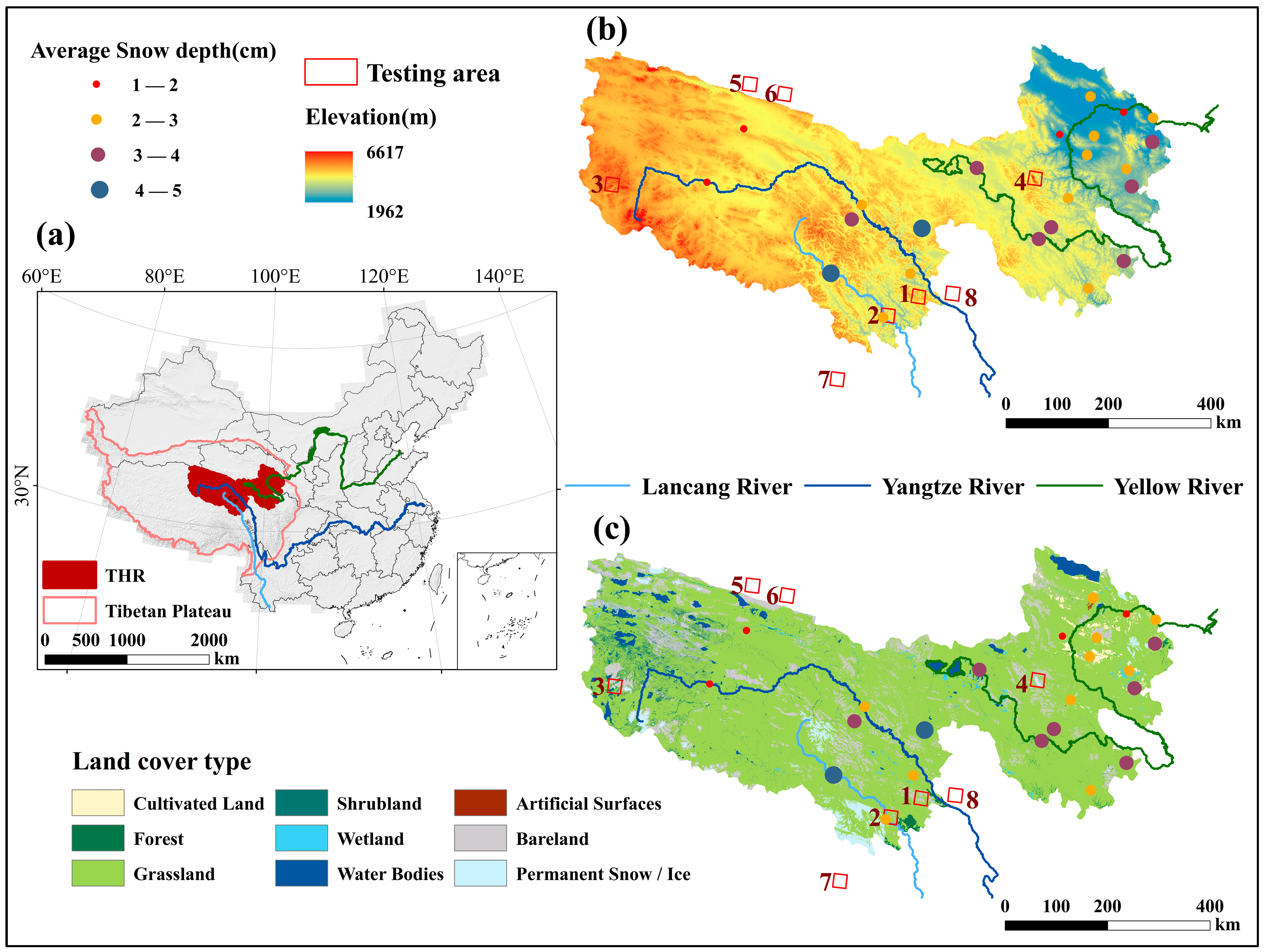
The THR is located in the northeastern part of the TP, around 31.55°–37.14°N and 89.42°–102.44°E, covering an area of approximately 3.75 × 10⁵ km2. It is bordered to the north by the Kunlun Mountains and the Qaidam Basin, to the west by the Hoh Xili Mountains and adjacent to the northern TP, to the southwest by the Tanggula Mountains, with the Bayan Har Mountains running southeast–northwest through the hinterland, and to the east by the eastern edge of the TP. As shown in Figure 2, the terrain is dominated by plateaus and mountains, with altitudes ranging from 1962 to 6617 m. The terrain is undulating, with an overall distribution of high west and low east. The climate is characterized by a typical plateau continental climate, with no significant variance between seasons and a large temperature difference between daytime and nighttime, with an average annual temperature of approximately 2 °C and an average annual precipitation of approximately 420 mm. In particular, snow cover is mainly accumulated in the central and western high-altitude areas, while snow cover distribution is relatively scattered in the eastern and southern parts; the annual average snowfall is approximately 150 mm, and the average number of snow cover days is approximately 90 [20]. The land cover is dominated by grassland and bare land, accounting for 90.56% of the total area, with a small area covered by forest land, accounting for 0.43% of the total area. Snow cover and glaciers are widespread, amounting to approximately 2.4 × 10³ km2. As the source of the Yangtze, Yellow, and Lancang rivers (upstream of the Mekong River), snow meltwater is an important source of water recharge for the rivers and is of great significance to industrial and agricultural water use and the development of the socioeconomic system in the downstream areas [46].

2.2. Data

2.2.1. MODIS Land Surface Reflectance Datasets

The MODIS Terra/Aqua Surface Reflectance Daily L2G Global 500 m and 1 km (MOD09GA V6.1) and MOD10A1.061 Terra Snow Cover Daily Global 500 m (MOD10A1 V6) datasets were obtained from the Moderate-Resolution Imaging Spectroradiometer (MODIS) onboard the Terra/Aqua satellite and downloaded from the Google Earth Engine (GEE) cloud computing platform (https://code.earthengine.google.com/, accessed on 10 October 2022). Both with a spatial resolution of 500 m and sinusoidal projection (SIN), MOD09GA V6.1 provides daily land surface reflectance data in 7 bands, while MOD10A1 V6 provides only daily land surface NDSI values (Equation (1)), without the binary snow cover (BSC) and fractional snow cover (FSC) values provided by previous versions. MOD09GA V6.1 and MOD10A1 V6 have been commonly used in studies on snow cover, owing to their relatively high temporal resolution and convenient acquisition [47,48,49,50].
Both MOD09GA V6.1 and MOD10A1 V6 were preprocessed on GEE. Cloud pixels in the remote sensing images were identified first and removed using GEE’s own cloud removal algorithm, and then radiometric calibration was performed, after which the projection was converted. Daily land surface reflectance and NDSI values (Equation (1)) were extracted for each station, and the land surface reflectance data were used to calculate the Normalized Difference Vegetation Index (NDVI, Equation (2)) and NDFSI values (Equation (3)), which were collectively used as auxiliary variables for snow cover discrimination.
N D S I = r e f 4 r e f 6 r e f 4 + r e f 6  
N D V I = r e f 2 r e f 1 r e f 2 + r e f 1
N D F S I = r e f 2 r e f 6 r e f 2 + r e f 6  
where r e f 1 , r e f 2 , r e f 4 , and r e f 6 are the land surface reflectance for the red, near-infrared, green, and shortwave infrared bands, respectively.

2.2.2. Land Surface Temperature Dataset

Land surface temperature (LST) data for 2001–2013 were obtained from the daily 1 km all-weather land surface temperature dataset for the Chinese landmass, and data on its surrounding areas were provided by the national Tibetan Plateau Data Center (TPDC, https://data.tpdc.ac.cn, accessed on 1 December 2022) [51]. The data have a temporal resolution of 2 times per day (daytime and nighttime) and a spatial resolution of 1 km. They were prepared by integrating Terra/Aqua MODIS LST products, GLDAS data, vegetation indices, and land surface albedo, with mean deviations of 0.09 K and −0.03 K and standard deviations of 1.45 K and 1.17 K during the daytime and nighttime, respectively [52].
LST is an important expression of the interaction between land surface and atmospheric energy [53,54], but it also has a complex feedback on ground–climate processes and is extremely sensitive to climate changes [51]. Therefore, LST is not only a sensitive indicator of climate change and a crucial prerequisite for understanding climate change patterns, but also a direct input parameter for numerous models. It is widely applicable to various fields, such as meteorology, climatology, environmental ecology, and hydrology [52,55]. The LST data used in this study reflect daytime and nighttime land surface temperature conditions; the land surface is the primary medium on which snow cover exists in the natural environment, and it may be sensitive and show intense responses to changes in snow cover [52].
In this study, the LST of each station during 2001 to 2013 was extracted, and the missing LST data (2004D_267-366/2004N_345-366/2012N_103-366) were corrected by establishing a regression relationship (Equations (4) and (5)), revised for daytime and nighttime with the available LST data and daily air temperature data at each station; LST was maintained as an auxiliary variable for snow cover discrimination. The daily air temperature data for 2001–2013 were obtained from the China Meteorological Forcing Dataset (CMFD, http://data.tpdc.ac.cn, accessed on 2 December 2022) provided by the TPDC, with high overall accuracy [56,57]. However, as the spatial resolution of the CMFD is low (0.1°), a significant difference was observed between station elevation and grid center elevation. Therefore, air temperature at the grid center was revised to the station using the daily vertical temperature gradient (−0.48 °C/100 m).
D = 0.8152 T + 17.406 ,   R 2 = 0.7147 , P < 0.05  
N = 0.9784 T 8.3193 , R 2 = 0.8982 , P < 0.05  
where D is the corrected daytime land surface temperature, N is the corrected nighttime land surface temperature, and T is the corrected air temperature of the SD observation station.

2.2.3. Snow Depth Dataset

Snow depth (SD) refers to the vertical depth from the surface of the snow cover to the ground. It is an important parameter for characterizing snow cover and a key element of routine meteorological observations. In this study, the Tibetan Plateau Station SD Dataset for the period 2001–2013 was obtained from the TPDC. There were 23 stations within the study region (Figure 2), and the observation data were obtained at 8 o’clock Beijing time and quality-controlled for accuracy with a daily temporal resolution. In this study, missing data for some years and months were excluded. We displayed the MODIS grid cells where the sites were located on Google Earth and excluded sites with relatively complex underlying surfaces. In the end, we retained only 15 sites that we considered relatively homogeneous for SCDM construction. The selected sites primarily consisted of grassland and bare land, and the terrain was relatively flat. Therefore, we believed that they could better represent the overall conditions of the MODIS pixels in which they were located. Furthermore, the observational data from the sites that were not selected would be used in the model testing phase. Furthermore, snow cover samples with SD greater than 2 cm were selected for model training to avoid the influence of mixed pixels. Then, the SD data were binarized. Specifically, if the SD was greater than 2 cm, the value was “1”, indicating snow cover; otherwise, the value was “0”, indicating a snow-free condition [35].

2.2.4. Other Dataset Sources

The digital elevation model Shuttle Radar Topography Mission (SRTM1 V3), with a spatial resolution of 30 m, was used in this study, having been downloaded through the GEE. The SRTM data were obtained from measurements conducted by the Endeavour space shuttle, jointly launched by the National Aeronautics and Space Administration (NASA) and the National Imagery and Mapping Agency (NIMA) in February 2000 [58]. The SRTM system onboard the Endeavour shuttle conducted a total of 222 h and 23 min of data collection. This mission covered over 80% of the Earth’s land surface, ranging from 60°N latitude to 56°S latitude, and included a comprehensive coverage of the entire territory of China; it is considered to be a reliable DEM source [59,60].
We used a 3 × 3 pixel moving window to calculate the mean elevation (MEAN), standard deviation (terrain standard deviation, STD), and relief amplitude (RA) within the window. The elevation coefficient of variation was calculated using STD/MEAN. Subsequently, we used the ”Aggregate” tool in ArcMap 10.5 to resample them to a spatial resolution of 500 m, matching the resolution of the MODIS pixels.
The dataset of snow cover days (SCD) was obtained from the National Cryosphere Desert Data Center (www.ncdc.ac.cn, accessed on 1 January 2023). The spatial resolution was 500 m, and the temporal resolution was 1 year, which can reflect the continuity of snow cover distribution in time to a certain extent and use it as the auxiliary variable.
Then, the auxiliary variables (Table 1) were matched to each station based on location and date attributes.

2.3. Random Forests Algorithm

Random forests (RF) is a machine learning algorithm proposed by Leo Breiman and Adele Cutler based on ensemble learning, through which missing values can be efficiently estimated and handled and model accuracy can be ensured [43]. The basic unit is the decision tree, which grows by autonomous sampling with put-back and the random selection of some input variables to discriminate between samples. The RF classification algorithm is a composite classification model composed of many individual classification models h X , Θ k , k = 1 , . It consists of independently and identically distributed random vectors { Θ k ) } . Through multiple rounds of training, it obtains a sequence of classification models h 1 X , h 2 X , , h k X . The final classification is determined by using a voting mechanism. The equation is as follows:
H x = a r g   max Y i = 1 k I h i x = Y  
where H x represents the composite classification model, h i x is an individual decision tree classification model, Y represents the output variable, and I · represents the indicator function.
The random feature selection in RF involves randomly choosing a small subset of input variables for splitting at each node. As a result, the node splits in the decision tree are determined based on these selected features, rather than by considering all features. Then, the trees are fully grown using the CART method without pruning, which helps reduce tree bias. Once the decision trees are constructed, a majority voting method is used to combine the predictions [61]. Obviously, a single decision tree is a weak classifier, and the collection of classification results from multiple decision trees forms a strong classifier, which is known as “Random Forests”. The “random” attribute is able to fully learn the mapping relationship between dependent and independent variables without overfitting, and the “forests” attribute is more accurate and resistant to interference than a single decision tree.
The generation of RF is determined by three main parameters: (1) the number of decision trees used to construct the random forests (Ntree), (2) the number of randomly selected factors when the decision trees are split (Mtry) [62], and the proportion of snow-free samples to snow-covered samples (ratio). The presence or absence of snow cover in this study is a simple binary classification problem, and the classification is based on the model of the voting results of all decision trees. We calculated the following metrics based on the confusion matrix to assess the model’s performance in snow cover discrimination: accuracy, Cohen’s kappa (kappa), F1 score (F1), area under the curve (AUC), precision, and recall. The meaning and calculation of each metric can be found in references [63,64].

3. Results

3.1. Parameters of the RF Model: Ntree, Mtry, and Ratio

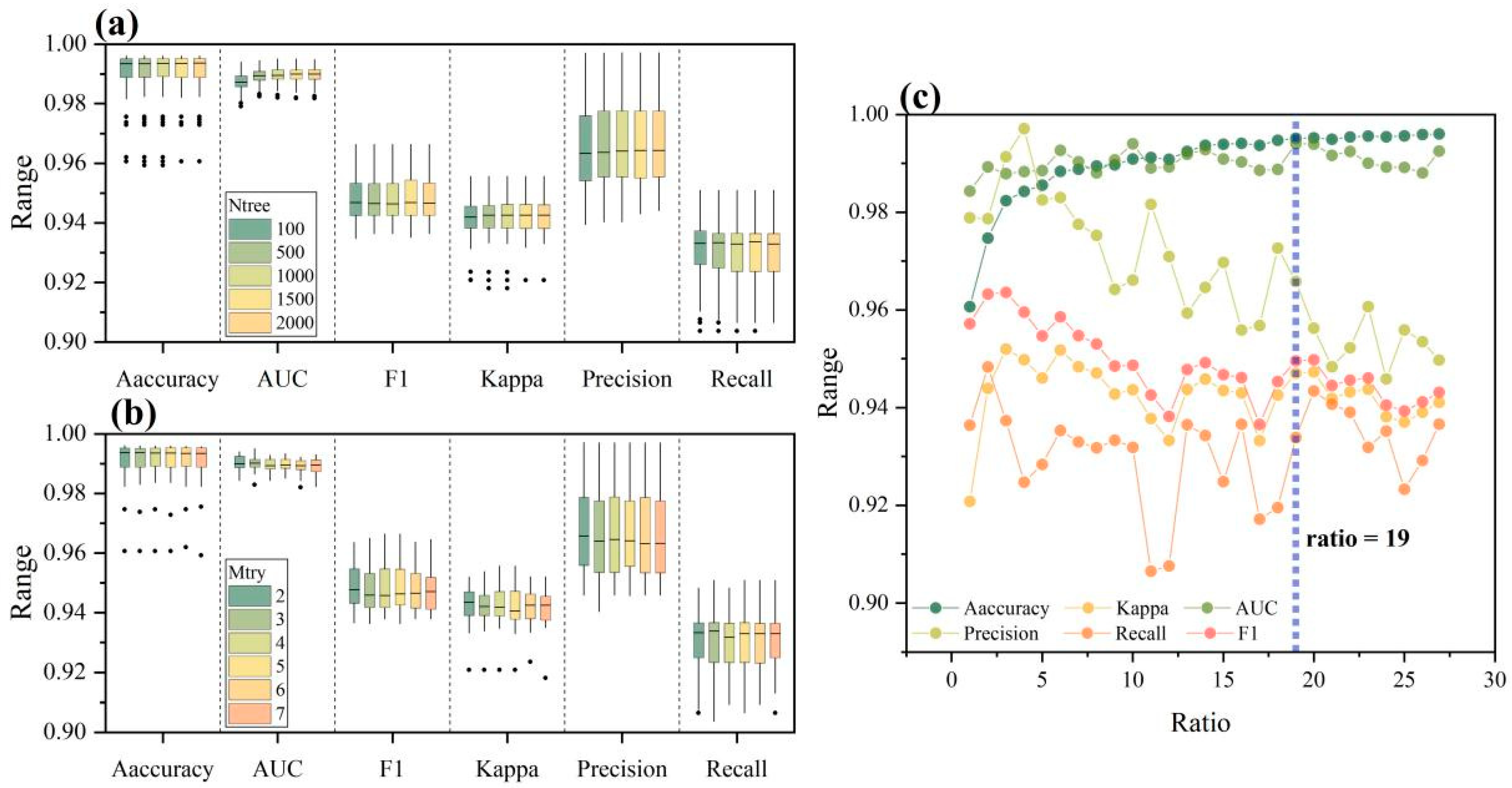
To enhance the performance and stability of the SCDM, a parameter search was conducted utilizing the grid search method. This involved systematically exploring all conceivable parameter values for the model. However, considering that the computational complexity of constructing an RF model escalates with elevated values of Ntree and Mtry, we designated specific values for Ntree (100, 500, 1000, 1500, and 2000), Mtry (ranging from 2 to 7 in increments of 1), and ratio (ranging from 1 to 26 in increments of 1, along with the inclusion of the maximum value of 26.91531 for ratio). By amalgamating permutations of these three parameters, a total of 810 models (5 × 6 × 27) were iteratively constructed to identify the optimal parameter configuration.
As depicted in Figure 3a, the mean values of accuracy, AUC, F1, kappa, and precision reached their peaks when Ntree was set to 1000. Concurrently, the mean value of recall was notably high. Hence, based on this observation (i.e., Ntree = 1000), as illustrated in Figure 3b, the highest mean values for accuracy, AUC, F1, kappa, precision, and recall were achieved when Mtry equaled 2. More specifically, as demonstrated in Figure 3c, with Ntree set at 1000 and Mtry at 2, a fluctuating trend was observed in the model metrics when ratio was less than 19. Accuracy oscillated within the range of 96.07–99.47%, kappa within 0.9208–0.9520, F1 within 0.9366–0.9636, AUC within 0.9843–0.9940, precision within 0.9559–0.9971, and recall within 0.9065–0.9483. However, the model metrics achieved stability when ratio exceeded or equaled 19. During this phase, accuracy fluctuated between 99.49% and 99.60%, kappa between 0.9370 and 0.9473, F1 between 0.9393 and 0.9498, AUC between 0.9881 and 0.9940, precision between 0.9459 and 0.9498, and recall between 0.9233 and 0.9434. Therefore, considering the metrics and the computational overhead of the model, the parameters Ntree, Mtry, and ratio within the SCDM were determined as 1000, 2, and 19, respectively.

3.2. Evaluation of the SCDM

The sample was divided into a training set (2001–2010) and a testing set (2011–2013) by year, and the training set was randomly divided in a 60%:40% ratio for model training and validation, respectively, 10 times. To avoid the influence of interactions between potential variables on the model performance, the factors were filtered through 10 intermediate models built using the varSelRF package in R. The final factor system (factors with ≥7 occurrences in the 10 intermediate models) was determined, which comprised eight factors (Figure 4). Subsequently, the final SCDM was constructed. The testing set, observation data from the remaining eight unselected sites in the THR, and a shallow snow cover sample set (SD ≤ 2 cm) were used to evaluate the generalization ability of the SCDM.
L o g i t P = ln P 1 P  
As shown in Table 2, the metrics for both the testing and training sets exhibited a high level of consistency. However, as observation data from the remaining eight unselected sites in the THR and the shallow snow cover sample set (SD ≤ 2 cm) from the training model were excluded, their metrics displayed a slight decline compared to the training set, and this decline was more pronounced in the latter. Nonetheless, the accuracy of all three sets of testing data remained generally satisfactory. Therefore, the SCDM can be used for snow discrimination in the THR.

3.3. Analysis of the Factors Influencing Snow Cover Distribution

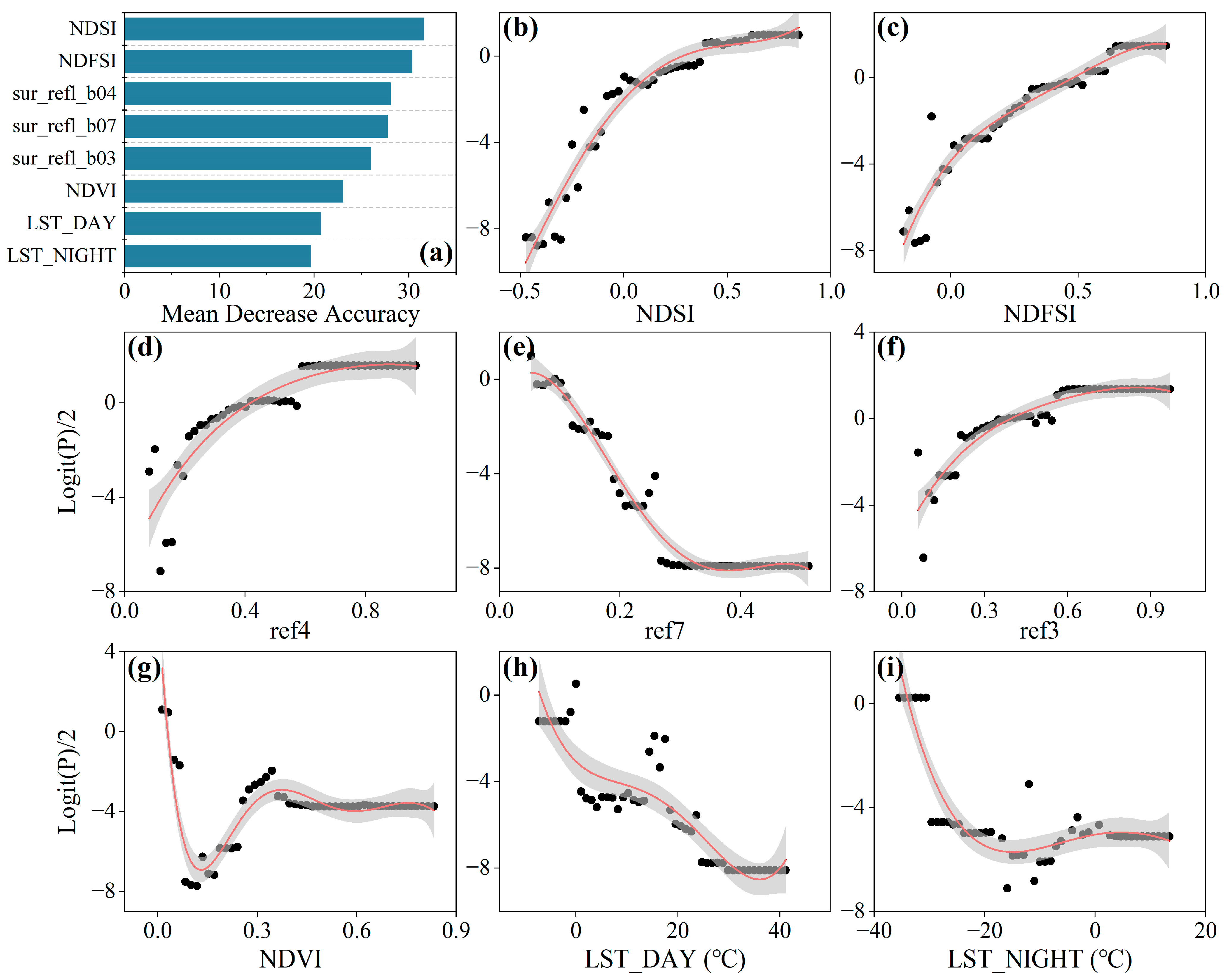
As shown in Figure 4, based on the SCDM, the importance of the factors affecting snow cover distribution in the THR was ranked, and the relationship between each factor and the snow cover distribution in the region was further clarified through a partial dependence plot.
When utilizing the SCDM for snow cover discrimination within the THR, snow cover indices emerged as pivotal components. Among these, the NDSI assumed the most influential role, followed by the Normalized Difference Forest Snow Index (NDFSI). Overall, the likelihood of snow cover distribution exhibited a positive correlation with both indices. Specifically, when the NDSI and NDFSI were below 0.39 and 0.62, respectively, the probability of widespread snow cover swiftly escalated with the elevation of these two indices. Beyond these thresholds, the likelihood of distributed snow cover stabilized at a high and consistent level. Similarly, the reflectance values of the green (ref4) and blue (ref3) bands also manifested a positive correlation with the probability of snow cover distribution. This correspondence is intrinsically linked to the conspicuous reflectance characteristics of snow cover within the visible-light spectrum. In particular, when ref4 and ref3 were below 0.58 and 0.56, respectively, the probability of extensive snow cover witnessed a rapid surge with the amplification of these two indices. Subsequently, the probability plateaued at a relatively elevated and unchanging level. Conversely, the likelihood of snow cover distribution exhibited a negative correlation with reflectance in the shortwave infrared band (ref7). This inverse relationship is attributable to the subdued reflectance properties of snow within the shortwave infrared spectrum. When ref7 descended below 0.26, the probability exhibited a precipitous decrease in tandem with rising ref7 values. Conversely, when ref7 surpassed 0.26, the probability dwindled to a relatively low and consistent state. In the broader picture, the spectral insights garnered from snow cover proved adept at differentiating between snow-covered and snow-free areas. This attribute underscores the significance of spectral information as a vital auxiliary variable in snow cover discrimination. Furthermore, the Normalized Difference Vegetation Index (NDVI) played a key role in snow cover discrimination owing to its inverse correlation with the probability of snow distribution. When the NDVI surpassed 0, the probability experienced an initial sharp decline, reaching its nadir at roughly NDVI 0.12, before slightly rebounding. Beyond an NDVI threshold of 0.36, the probability remained at a low and steady level.
Land surface temperature (LST) also contributed to the discrimination of snow cover within the THR, with both LST_DAY and LST_NIGHT displaying negative correlations with the probability of snow cover distribution. Notably, when LST_DAY was below 0 °C and LST_NIGHT was less than −29 °C, the probability exhibited a relatively high and steady state. However, as the land surface temperature escalated, the probability experienced a rapid decline. A further reduction in probability was observed when LST_DAY exceeded 24 °C and LST_NIGHT surpassed 0.7 °C, resulting in an exceedingly low and stable probability.
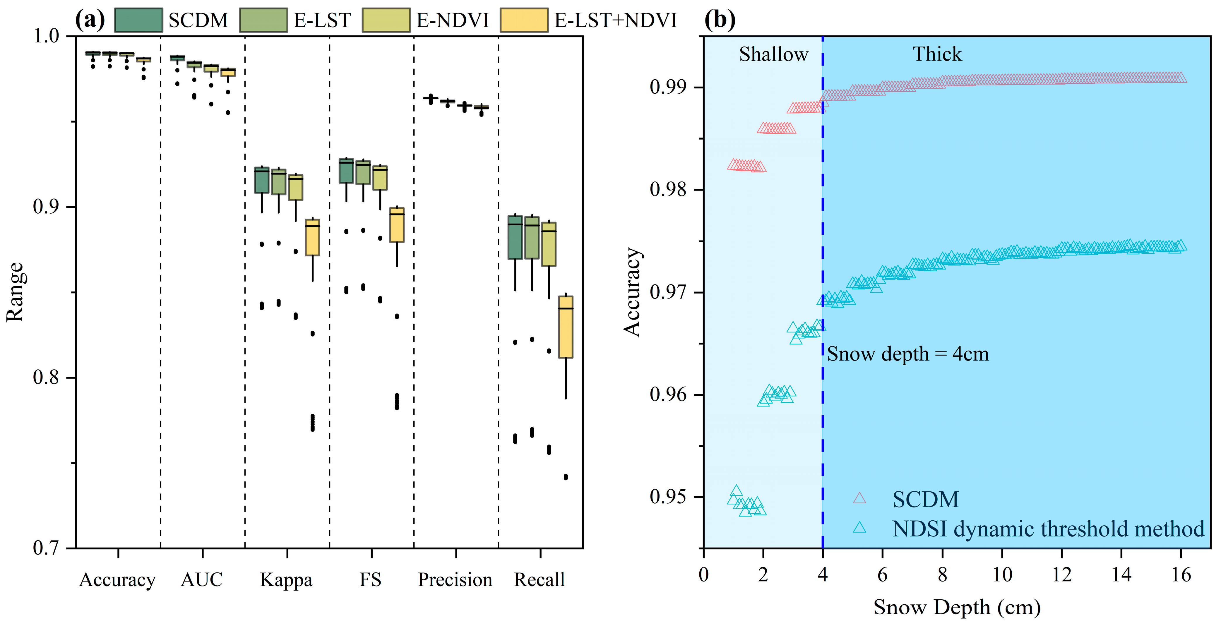
As illustrated in Figure 5a, the impacts of the NDVI and LST on the performance of the SCDM were quantified across samples featuring varying SD. The inclusion of the NDVI and LST independently improved the average accuracy of the SCDM by 0.05% and 0.01%, respectively. When the NDVI and LST were simultaneously considered, the average accuracy surged by 0.39%. Correspondingly, the area under the curve (AUC) increased by 0.64%, 0.4%, and 0.90%; kappa increased by 0.46%, 0.08%, and 3.63%; F1 score (FS) increased by 0.43%, 0.07%, and 3.43%; precision increased by 0.43%, 0.17%, and 0.53%; and recall increased by 0.42%, 0.002%, and 5.56%. Evidently, in the context of snow cover discrimination within the THR, the NDVI exerted a more substantial influence than LST. Moreover, the improvement in model performance by incorporating both the NDVI and LST was notable.

3.4. Model Discrimination Capability of Snow Cover at Different Snow Depths

To assess the accuracy of the SCDM in discriminating various SDs within the THR, a comparison was made with the dynamic thresholds method. This method was selected to discriminate snow cover by configuring dynamic thresholds as follows [65]: snow cover samples with SD ranging from 1 to 16 cm, in increments of 0.1 cm, were combined with snow-free samples based on the predetermined ratio. The threshold spanned from −1 to 1 in increments of 0.01. If the NDSI was greater than or equal to the threshold and the reflectance of ref2 and ref4 exceeded 0.11 and 0.1, respectively, snow cover was designated as accumulating; otherwise, it was considered to be non-accumulating. Notably, this method incorporated the temporal variability of the NDSI threshold, setting it apart from the SNOMAP approach (which employs a fixed NDSI threshold of 0.4) introduced by Hall [24].
As depicted in Figure 5b, when the SD exceeded 1 cm, the discrimination accuracy generally exhibited an upward trend with increasing SD, eventually stabilizing. Specifically, for the dynamic threshold method, the average discrimination accuracy reached 95.88% for SD ≤ 4 cm and 98.30% for SD > 4 cm. Meanwhile, for the SCDM, the average discrimination accuracy was 98.54% and 99.04% for the same respective ranges. Notably, irrespective of thick or thin SD, the latter method proved significantly superior (p < 0.01) to the former. This substantiates the suitability of the SCDM for effectively discriminating snow cover extent within the THR.

4. Discussion

4.1. Temporal Comparison with Other Snow Cover Products

To further clarify the capability of the SCDM to discriminate snow cover in the THR, we attempted to compare the accuracy of the SCDM with other snow cover products that have been used commonly. We downloaded the “Long-term series of daily snow depth dataset over the Northern Hemisphere based on machine learning” developed by Che (SDML_Che, https://cstr.cn/18406.11.Snow.tpdc.271701, accessed on 1 May 2023) [66], the MODIS daily cloud-free snow cover area product for Sanjiangyuan from 2000 to 2019 developed by Hao (MODIS_Hao, http://www.ncdc.ac.cn, accessed on 2 May 2023) [67], and the “MODIS daily cloud-free snow cover product over the Tibetan Plateau” developed by Qiu (MODIS_Qiu, https://www.scidb.cn, accessed on 2 May 2023) [68]. We extracted the number of snow cover samples for all 23 stations in the THR on a daily basis, station by station, and matched them with the full samples. Subsequently, SDML_Che was binarized (SD > 2 cm:1; SD ≤ 2 cm:0) with reference to Che’s method [35], and the missing values were removed. Additionally, the extracted values from the other two snow cover products were also binarized.
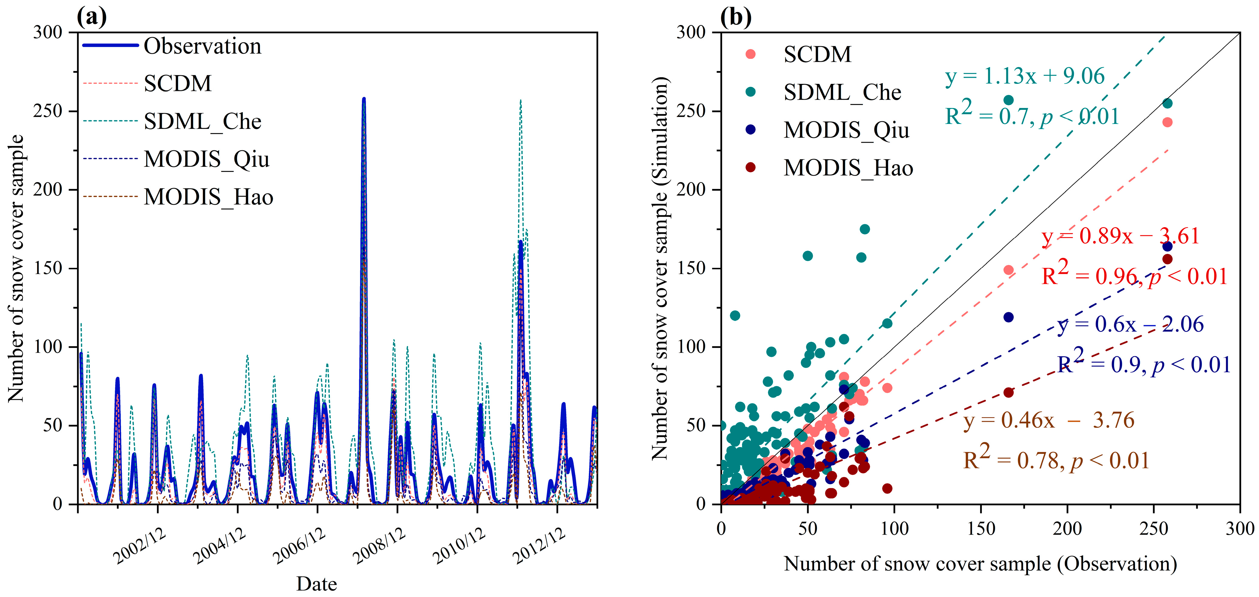
As shown in Figure 6a, the simulated monthly snow cover sample count based on the SCDM presented strong consistency with the observed values. Specifically, as shown in Figure 6b, the R2 between the SCDM results and the observed values was 0.96 (p < 0.01), indicating the best performance. The R2 between SDML_Che, MODIS_Qiu, MODIS_Hao, and the observed values was 0.7 (p < 0.01), 0.9 (p < 0.01), and 0.78 (p < 0.01), respectively. Therefore, in terms of the time series, the SCDM showed the best performance.
It is important to note that the spatial resolution of SDML_Che is 0.25° (≈25 km). We directly used the snow depth values within the 0.25° pixel where the snow depth monitoring station was located, assuming that the snow depth was uniform within this 0.25° × 0.25° range. This assumption introduced considerable uncertainty. Therefore, we discussed the relationship between SDML_Che and the observational data for different seasons. As shown in Figure S2, the correlation coefficients between SDML_Che and the observational data were relatively high in summer (June–August) and winter (December–February), at 0.94 (p < 0.05) and 0.81 (p < 0.05), respectively. This was because the snow cover was extensive in winter and limited in summer, resulting in relatively consistent snow cover distribution within the same pixel range. However, in spring (March–May) and autumn (September–November), the correlation coefficients between SDML_Che and the observational data were lower, at 0.62 (p < 0.05) and 0.59 (p < 0.05), respectively. This was due to spring being the snow melt period and autumn being the snow accumulation period, resulting in relatively heterogeneous snow cover distribution within the same pixel range and, hence, greater uncertainty. Nevertheless, overall, SDML_Che showed good consistency with the observational data. Therefore, if it was solely used for snow cover discrimination and time-series analysis, we believed it was reasonable. However, due to its lower spatial resolution, it could not be used for the subsequent spatial analysis and comparisons.

4.2. Spatial Comparison with Other Snow Cover Products

The SCDM was employed to assess snow cover discrimination across different regions, encompassing diverse terrain, imaging times, and snow cover fractions. To evaluate the spatial discrimination capability of the SCDM, four areas within the study region and four areas outside the study region were selected (as depicted in Figure 2 and Figure 7(a1–h1)). In the process of selecting Landsat-7 ETM images corresponding to the testing areas, careful consideration was given to factors such as spatial/temporal heterogeneity, known to influence the generalization ability of the model. In this manner, the spatial generalization capacity of the SCDM was quantitatively assessed to the maximum extent. The specific methodology is outlined as follows: First, Landsat-7 ETM images were selected and subjected to automatic classification using the ISODATA algorithm to extract snow cover, generating binary images. These images were then resampled to a spatial resolution of 500 m (Figure 7(a2–h2)) and used as the reference “true values”. Next, auxiliary variables corresponding to the same dates and regions (selected by the SCDM) were extracted. The SCDM was then applied, binarizing the model output and generating binary images (Figure 7(a3–h3)) (SCDM). Additionally, the MODIS_Qiu (Figure 7(a4–h4)) and MODIS_Hao (Figure 7(a5–h5)) datasets were extracted for spatial comparison.
As shown in Figure 7(a1–d1), four testing areas within the study region were selected. In comparison to the MODIS_Qiu and MODIS_Hao datasets, the SCDM exhibited the highest overall discrimination accuracy. Among the testing areas, the highest accuracy (98%) was achieved in testing area 4. This was followed by testing areas 1 and 2, with accuracies of 97.7% and 87.8%, respectively. Notably, the snow cover discrimination accuracy for testing area 3 was relatively lower. This was attributed to the presence of discontinuous and shallow snow cover in the northeastern part of the area, coupled with its smaller distribution area. This information was challenging to capture in MODIS imagery, resulting in unsuccessful discrimination. MODIS_Qiu and MODIS_Hao faced similar challenges. In contrast, the SCDM outperformed MODIS_Qiu and MODIS_Hao in snow cover discrimination within the study region.
As shown in Figure 7(e1–h1), four testing areas outside the study region were also selected. While the overall accuracy of the SCDM decreased compared to the testing areas within the region, it still exhibited superior performance over MODIS_Qiu and MODIS_Hao. Among these areas, the highest discrimination accuracy (95.2%) was achieved in testing area 8. This was followed by testing areas 5 and 7, with accuracies of 95.2% and 88.4%, respectively. However, the accuracy was relatively lower in testing area 6, which was primarily attributable to the misclassification of snow-free areas in central valleys as snow cover, resulting in some degree of overestimation. Nevertheless, MODIS_Qiu and MODIS_Hao tended to underestimate snow cover—especially the latter, which exhibited significant underestimation.
In summary, both within and outside the study region, the SCDM exhibited superior capability in snow cover discrimination compared to MODIS_Qiu and MODIS_Hao.

4.3. Uncertainties and Limitations

To ensure the authenticity and accuracy of the training set, we attempted to construct the SCDM at the station scale (or pixel scale). Given the intricate nature of underlying surfaces and the potential for mixed pixels in regions with shallow snow cover, we chose to include only thick snow cover samples (SD > 2 cm) from 15 relatively homogeneous sites for training the SCDM. While the accuracy of the SCDM at the station scale (Figure 6) and local spatial scale (Figure 7) exceeded that of other snow cover products, it is important to acknowledge that the limited number of sites (15) substantially constrained the generalization capacity of the model. This limitation may serve as a significant factor affecting the SCDM, especially in areas with greater heterogeneity than the selected sites, where potential shortcomings in snow cover discrimination may arise. Additionally, the predominant land cover types within the THR consist of grassland and bare land (as outlined in Section 2.1). The SCDM was specifically developed for these particular underlying surface types. Consequently, its snow cover discrimination capability might be constrained in regions with different land cover characteristics, such as forests or artificial surfaces. In contrast, the unselected sites were primarily located in urban areas, where the land cover within the MODIS pixels was more heterogeneous. This heterogeneity led to missed detection of snow cover by the SCDM. Additionally, when the observed snow depth was ≤2 cm, it implied that, at that time, the station and its surroundings likely had predominantly shallow snow cover and a lower snow cover fraction. Consequently, the issue of mixed pixels was unavoidable, which may have led to the presence of shallow snow cover being underestimated. Even if shallow snow cover was observed, the spectral response of the MODIS pixel to which it belonged may not have been very strong. So, at this point, the representativeness of binary classification pixels may be a significant source of uncertainty. Furthermore, due to the time difference between the MOD09GA data overpass time (local time at 10:30 every day) and the station observation time (Beijing time at 8:00 every day), snow cover may have undergone melting or accumulation during this period, also resulting in missed detection and false detection. As part of our future efforts, we intend to enhance the temporal and spatial density of site observations in order to expand the size of the training set. This expansion would aim to strengthen the performance of the SCDM in diverse land cover type areas. Through these endeavors, we hope to address the model’s limitations and further improve its applicability to a broader range of scenarios.
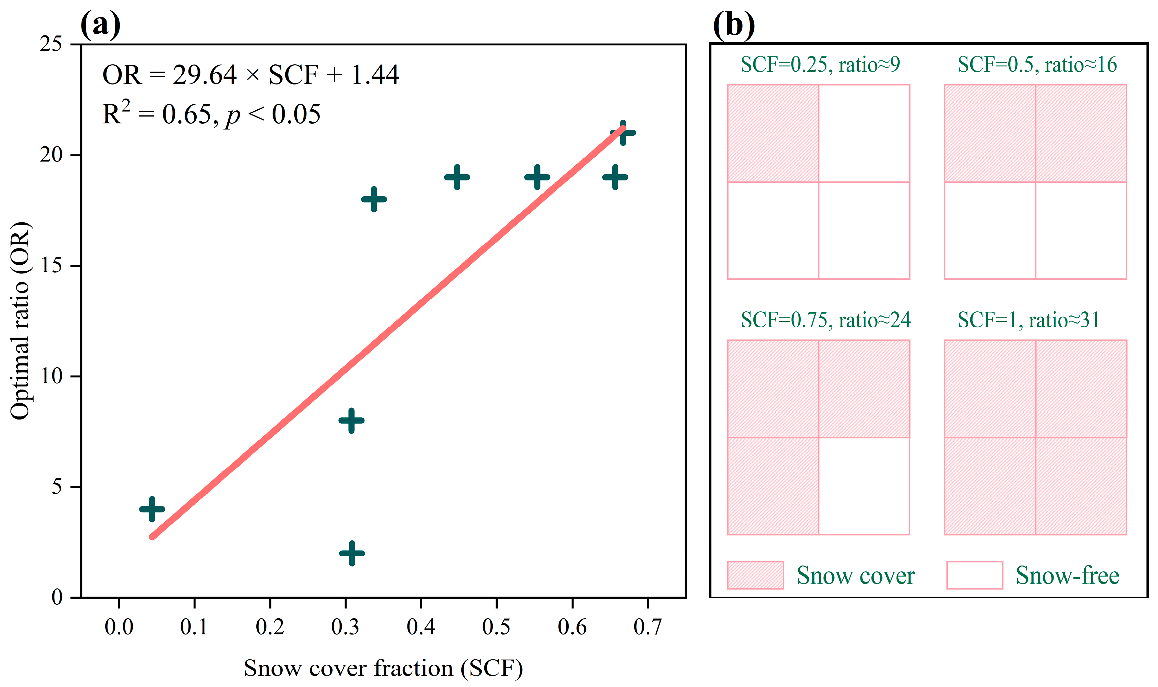
During the development of the SCDM, we identified the ratio parameter as a crucial factor influencing the model’s performance. In the parameter optimization stage, the highest overall performance (on average) of the SCDM was achieved at ratio = 19. However, during the onsite validation stage, the situation was different. In other words, the SCDM did not necessarily present the highest accuracy at ratio = 19 in different validation areas. This disparity was assumed to be possibly linked to the snow cover fraction (SCF) within the validation areas. Hence, SCF was calculated for each area based on the results of Landsat-7 ETM image classification, and the optimal ratio (OR) was further subjected to a simple linear regression analysis. As depicted in Figure 8a, a significant positive correlation emerged between these two variables (p < 0.05), with an R2 value of 0.65. This finding suggests that the optimal ratio for the SCDM tends to increase with a corresponding increase in SCF. Therefore, different ratio values are recommended for different SCFs, as illustrated in Figure 8b. It is essential to note that the optimal ratio was not 1 but approximately 16 when the SCF reached 0.5. This peculiarity might stem from the greater complexity of surface characteristics in snow-free areas compared to snow-covered areas. Consequently, the SCDM might require a larger number of snow-free samples to effectively capture the distinct surface features in such regions.
Furthermore, the assumptions of the confusion matrix (such as pure pixels) are often challenging to meet. Large-scale remote sensing mapping often involves issues such as mixed pixels, representativeness of defined classes, and matching ground data with remote sensing data. These assumptions are more difficult to satisfy, especially with 500 m spatial resolution MODIS data. However, currently, the confusion matrix is the core method for accuracy assessment in remote sensing image classification, because it can describe classification accuracy and reveal the confusion between classes. Therefore, regarding this issue, in our future work, we will attempt to use higher-spatial-resolution remote sensing images or employ methods like pixel unmixing to enhance the representativeness and credibility of the defined classes, reducing the uncertainty in this evaluation system.

5. Conclusions

In this study, based on the SD observation data from the stations, the RF algorithm was used to construct an SCDM for the THR, taking into account land surface reflectance, normalized indices, and LST. In addition, factors affecting the snow cover distribution in the area and the simulation capability of the SCDM were systematically analyzed. The main conclusions are as follows:
(1)
The model performance was optimal when the parameters Ntree, Mtry, and ratio were set at 1000, 2, and 19, respectively. There was a significant positive correlation between OR and SCF (p < 0.05), with an R2 value of 0.65. Compared with other snow cover products, the SCDM showed superior performance for snow cover discrimination, whether at the pixel scale or the local spatial scale.
(2)
The spectral information of snow cover was an important auxiliary variable in snow cover discrimination. For example, the NDSI, NDFSI, ref4, ref3, ref7, and NDVI appeared as crucial indicators for the SCDM, and a more pronounced improvement in model performance could be achieved by considering both the NDVI and LST.
(3)
Specifically, the average discrimination accuracy of the dynamic threshold method was 95.88% when SD ≤ 4 cm and 98.30% when SD > 4 cm, and the corresponding average discrimination accuracy of the SCDM was 98.54% and 99.04%. Irrespective of thick (SD > 4 cm) or thin (SD ≤ 4 cm) snow cover, the SCDM showed significantly higher performance (p < 0.01) than the traditional dynamic threshold method. Therefore, the SCDM is more suitable for discriminating snow cover’s extent in the THR.

Supplementary Materials

The following supporting information can be downloaded at: https://www.mdpi.com/article/10.3390/rs15194644/s1, Figure S1: (a) The relationship between temperature and LST_DAY. (b)The relationship between temperature and LST_NIGHT; Figure S2: Comparison of SDML_Che data with site observations in different seasons: (a) spring; (b) summer; (c) autumn; (d) winter; Table S1: Variable selection results of 10 intermediate models.

Author Contributions

Conceptualization, R.H., Q.Z. and Z.J.; methodology, R.H.; software, R.H.; validation, Y.Q., Q.Z. and Y.C.; formal analysis, Y.Q. and Z.J.; investigation, Y.Q., Q.Z. and Y.C.; resources, Q.Z., data curation, R.H. and Z.J.; writing—original draft preparation, R.H.; writing—review and editing, R.H., Y.Q., Q.Z. and Y.C.; visualization, R.H. and Z.J.; supervision, Q.Z.; project administration, Q.Z. and Y.Q.; funding acquisition, Q.Z. and Y.C. All authors have read and agreed to the published version of the manuscript.

Funding

This study was jointly funded by a joint research program of the Three-Rivers-Source National Park (LHZX-2020-10), the National Natural Science Foundation of China (Grants No. 41871059 and 42001030), the Natural Science Foundation of Gansu Province (23JRRA597), and the State Key Laboratory of Cryospheric Science (SKLCS-ZZ-2023).

Data Availability Statement

Not applicable.

Acknowledgments

The authors gratefully acknowledge the support of various foundations.

Conflicts of Interest

The authors declare no conflict of interest.

References

  1. Huang, X.; Deng, J.; Wang, W.; Feng, Q.; Liang, T. Impact of climate and elevation on snow cover using integrated remote sensing snow products in Tibetan Plateau. Remote Sens. Environ. 2017, 190, 274–288. [Google Scholar] [CrossRef]
  2. Allchin, M.I.; Dery, S.J. A spatio-temporal analysis of trends in Northern Hemisphere snow-dominated area and duration, 1971–2014. Ann. Glaciol. 2017, 58, 21–35. [Google Scholar] [CrossRef]
  3. Armstrong, R.L.; Brodzik, M.J. Recent Northern Hemisphere snow extent: A comparison of data derived from visible and microwave satellite sensors. GeoRL 2001, 28, 3673–3676. [Google Scholar] [CrossRef]
  4. Wang, Y.; Huang, X.; Liang, H.; Sun, Y.; Feng, Q.; Liang, T. Tracking Snow Variations in the Northern Hemisphere Using Multi-Source Remote Sensing Data (2000–2015). Remote Sens. 2018, 10, 136. [Google Scholar] [CrossRef]
  5. Tang, Z.; Wang, X.; Wang, J.; Wang, X.; Li, H.; Jiang, Z. Spatiotemporal Variation of Snow Cover in Tianshan Mountains, Central Asia, Based on Cloud-Free MODIS Fractional Snow Cover Product, 2001–2015. Remote Sens. 2017, 9, 1045. [Google Scholar] [CrossRef]
  6. Natali, S.M.; Watts, J.D.; Rogers, B.M.; Potter, S.; Ludwig, S.M.; Selbmann, A.-K.; Sullivan, P.F.; Abbott, B.W.; Arndt, K.A.; Birch, L.; et al. Large loss of CO2 in winter observed across the northern permafrost region. Nat. Clim. Chang. 2019, 9, 852–857. [Google Scholar] [CrossRef]
  7. Bintanja, R.; Andry, O. Towards a rain-dominated Arctic. Nat. Clim. Chang. 2017, 7, 263–267. [Google Scholar] [CrossRef]
  8. Arnold, J.G.; Fohrer, N. SWAT2000: Current capabilities and research opportunities in applied watershed modelling. Hydrol. Process. 2005, 19, 563–572. [Google Scholar] [CrossRef]
  9. Douville, H.; Royer, J.F. Sensitivity of the Asian summer monsoon to an anomalous Eurasian snow cover within the Meteo-France GCM. Clim. Dyn. 1996, 12, 449–466. [Google Scholar] [CrossRef]
  10. Chen, J.; Sheng, Y.; Wu, Q.; Zhao, L.; Li, J.; Zhao, J. Effects of Seasonal Snow Cover on Hydrothermal Conditions of the Active Layer in the Northeastern Qinghai-Tibet Plateau. Cryosphere Discuss 2016, 1–22. [Google Scholar] [CrossRef]
  11. Wu, T.W.; Qian, Z.A. The relation between the Tibetan winter snow and the Asian summer monsoon and rainfall: An observational investigation. J. Clim. 2003, 16, 2038–2051. [Google Scholar] [CrossRef]
  12. Nan, S.; Zhao, P.; Yang, S.; Chen, J. Springtime tropospheric temperature over the Tibetan Plateau and evolutions of the tropical Pacific SST. J. Geophys. Res. Atmos. 2009, 114. [Google Scholar] [CrossRef]
  13. Notarnicola, C. Hotspots of snow cover changes in global mountain regions over 2000–2018. Remote Sens. Environ. 2020, 243, 111781. [Google Scholar] [CrossRef]
  14. O’Gorman, P.A. Contrasting responses of mean and extreme snowfall to climate change. Nature 2014, 512, 416–418. [Google Scholar] [CrossRef] [PubMed]
  15. Nicolet, G.; Eckert, N.; Morin, S.; Blanchet, J. Decreasing spatial dependence in extreme snowfall in the French Alps since 1958 under climate change. J. Geophys. Res.-Atmos. 2016, 121, 8297–8310. [Google Scholar] [CrossRef]
  16. Zou, Y.F.; Sun, P.; Ma, Z.C.; Lv, Y.F.; Zhang, Q. Snow Cover in the Three Stable Snow Cover Areas of China and Spatio-Temporal Patterns of the Future. Remote Sens. 2022, 14, 3098. [Google Scholar] [CrossRef]
  17. Changnon, S.A.; Changnon, D. A spatial and temporal analysis of damaging snowstorms in the United States. Nat. Hazards 2006, 37, 373–389. [Google Scholar] [CrossRef]
  18. Barnett, T.P.; Dumenil, L.; Schlese, U.; Roeckner, E.; Latif, M. The Effect of Eurasian Snow Cover on Regional and Global Climate Variations. J. Atmos. Sci. 1989, 46, 661–685. [Google Scholar] [CrossRef]
  19. Hansen, J.; Nazarenko, L. Soot climate forcing via snow and ice albedos. Proc. Natl. Acad. Sci. USA 2004, 101, 423–428. [Google Scholar] [CrossRef]
  20. Chen, L.; Zhang, W.; Yi, Y.; Zhang, Z.; Chao, S. Long Time-Series Glacier Outlines in the Three-Rivers Headwater Region from 1986 to 2021 Based on Deep Learning. IEEE J. Sel. Top. Appl. Earth Obs. Remote Sens. 2022, 15, 5734–5752. [Google Scholar] [CrossRef]
  21. Kaushik, S.; Joshi, P.K.; Singh, T. Development of glacier mapping in Indian Himalaya: A review of approaches. Int. J. Remote Sens. 2019, 40, 6607–6634. [Google Scholar] [CrossRef]
  22. Garg, S.; Shukla, A.; Garg, P.K.; Yousuf, B.; Shukla, U.K.; Lotus, S. Revisiting the 24 year (1994–2018) record of glacier mass budget in the Suru sub-basin, western Himalaya: Overall response and controlling factors. Sci. Total Environ. 2021, 800, 149533. [Google Scholar] [CrossRef]
  23. Dozier, J. Spectral Signature of Alpine Snow Cover from the Landsat Thematic Mapper. Remote Sens. Environ. 1989, 28, 9–22. [Google Scholar] [CrossRef]
  24. Hall, D.K.; Riggs, G.A.; Salomonson, V.V. Development of methods for mapping global snow cover using moderate resolution imaging spectroradiometer data. Remote Sens. Environ. 1995, 54, 127–140. [Google Scholar] [CrossRef]
  25. Sood, V.; Singh, S.; Taloor, A.K.; Prashar, S.; Kaur, R. Monitoring and mapping of snow cover variability using topographically derived NDSI model over north Indian Himalayas during the period 2008-19. Appl. Comput. Geosci. 2020, 8, 100040. [Google Scholar] [CrossRef]
  26. Haerer, S.; Bernhardt, M.; Siebers, M.; Schulz, K. On the need for a time- and location-dependent estimation of the NDSI threshold value for reducing existing uncertainties in snow cover maps at different scales. Cryosphere 2018, 12, 1629–1642. [Google Scholar] [CrossRef]
  27. Jing, Y.; Shen, H.; Li, X.; Guan, X. A Two-Stage Fusion Framework to Generate a Spatio-Temporally Continuous MODIS NDSI Product over the Tibetan Plateau. Remote Sens. 2019, 11, 2261. [Google Scholar] [CrossRef]
  28. Wang, X.-Y.; Wang, J.; Jiang, Z.-Y.; Li, H.-Y.; Hao, X.-H. An Effective Method for Snow-Cover Mapping of Dense Coniferous Forests in the Upper Heihe River Basin Using Landsat Operational Land Imager Data. Remote Sens. 2015, 7, 17246–17257. [Google Scholar] [CrossRef]
  29. Hao, X.; Huang, G.; Che, T.; Ji, W.; Sun, X.; Zhao, Q.; Zhao, H.; Wang, J.; Li, H.; Yang, Q. The NIEER AVHRR snow cover extent product over China: A long-termdaily snow record for regional climate research. Earth Syst. Sci. Data 2021, 13, 4711–4726. [Google Scholar] [CrossRef]
  30. Zhang, H.; Zhang, F.; Zhang, G.; Che, T.; Yan, W.; Ye, M.; Ma, N. Ground-based evaluation of MODIS snow cover product V6 across China: Implications for the selection of NDSI threshold. Sci. Total Environ. 2019, 651, 2712–2726. [Google Scholar] [CrossRef] [PubMed]
  31. Hall, D.K.; Riggs, G.A.; Salomonson, V.V.; DiGirolamo, N.E.; Bayr, K.J. MODIS snow-cover products. Remote Sens. Environ. 2002, 83, 181–194. [Google Scholar] [CrossRef]
  32. Yang, J.; Jiang, L.; Shi, J.; Wu, S.; Sun, R.; Yang, H. Monitoring snow cover using Chinese meteorological satellite data over China. Remote Sens. Environ. 2014, 143, 192–203. [Google Scholar] [CrossRef]
  33. Palermo, G.; Raparelli, E.; Tuccella, P.; Orlandi, M.; Marzano, F.S. Using Artificial Neural Networks to Couple Satellite C-Band Synthetic Aperture Radar Interferometry and Alpine3D Numerical Model for the Estimation of Snow Cover Extent, Height, and Density. IEEE J. Sel. Top. Appl. Earth Obs. Remote Sens. 2023, 16, 2868–2888. [Google Scholar] [CrossRef]
  34. Foster, J.L.; Chang, A.T.C.; Hall, D.K. Comparison of snow mass estimates from prototype passive microwave snow algorithm, a revised algorithm and a snow depth climatology. Remote Sens. Environ. 1997, 62, 132–142. [Google Scholar] [CrossRef]
  35. Che, T.; Li, X.; Jin, R.; Armstrong, R.; Zhang, T. Snow depth derived from passive microwave remote-sensing data in China. In Proceedings of the International Symposium on Snow Science, Moscow, Russia, 3–7 September 2008; pp. 145–154. [Google Scholar]
  36. Liu, R.; Wen, J.; Wang, X.; Wang, Z.; Liu, Y.; Zhang, M. Estimates of Daily Evapotranspiration in the Source Region of the Yellow River Combining Visible/Near-Infrared and Microwave Remote Sensing. Remote Sens. 2021, 13, 53. [Google Scholar] [CrossRef]
  37. Jordan, M.I.; Mitchell, T.M. Machine learning: Trends, perspectives, and prospects. Science 2015, 349, 255–260. [Google Scholar] [CrossRef]
  38. Mao, K.; Wang, H.; Shi, J.; Heggy, E.; Wu, S.; Bateni, S.M.; Du, G. A General Paradigm for Retrieving Soil Moisture and Surface Temperature from Passive Microwave Remote Sensing Data Based on Artificial Intelligence. Remote Sens. 2023, 15, 1793. [Google Scholar] [CrossRef]
  39. Du, B.; Mao, K.; Bateni, S.M.; Meng, F.; Wang, X.M.; Guo, Z.; Jun, C.; Du, G. A Novel Fully Coupled Physical–Statistical–Deep Learning Method for Retrieving Near-Surface Air Temperature from Multisource Data. Remote Sens. 2022, 14, 5812. [Google Scholar] [CrossRef]
  40. He, G.; Xiao, P.; Feng, X.; Zhang, X.; Wang, Z.; Chen, N. Extracting Snow Cover in Mountain Areas Based on SAR and Optical Data. IEEE Geosci. Remote Sens. Lett. 2015, 12, 1136–1140. [Google Scholar] [CrossRef]
  41. Dobreva, I.D.; Klein, A.G. Fractional snow cover mapping through artificial neural network analysis of MODIS surface reflectance. Remote Sens. Environ. 2011, 115, 3355–3366. [Google Scholar] [CrossRef]
  42. Kuter, S.; Akyurek, Z.; Weber, G.-W. Retrieval of fractional snow covered area from MODIS data by multivariate adaptive regression splines. Remote Sens. Environ. 2018, 205, 236–252. [Google Scholar] [CrossRef]
  43. Breiman, L. Bagging predictors. Mach. Learn. 1996, 24, 123–140. [Google Scholar] [CrossRef]
  44. Kuter, S. Completing the machine learning saga in fractional snow cover estimation from MODIS Terra reflectance data: Random forests versus support vector regression. Remote Sens. Environ. 2021, 255, 112294. [Google Scholar] [CrossRef]
  45. Luo, J.; Dong, C.; Lin, K.; Chen, X.; Zhao, L.; Menzel, L. Mapping snow cover in forests using optical remote sensing, machine learning and time-lapse photography. Remote Sens. Environ. 2022, 275, 113017. [Google Scholar] [CrossRef]
  46. Li, Z.J.; Li, Z.X.; Feng, Q.; Wang, X.F.; Mu, Y.H.; Xin, H.J.; Song, L.L.; Gui, J.; Zhang, B.J.; Gao, W.D.; et al. Hydrological effects of multiphase water transformation in Three-River Headwaters Region, China. J. Hydrol. 2021, 601, 126662. [Google Scholar] [CrossRef]
  47. Painter, T.H.; Rittger, K.; McKenzie, C.; Slaughter, P.; Davis, R.E.; Dozier, J. Retrieval of subpixel snow covered area, grain size, and albedo from MODIS. Remote Sens. Environ. 2009, 113, 868–879. [Google Scholar] [CrossRef]
  48. Stillinger, T.; Roberts, D.A.; Collar, N.M.; Dozier, J. Cloud Masking for Landsat 8 and MODIS Terra Over Snow-Covered Terrain: Error Analysis and Spectral Similarity Between Snow and Cloud. Water Resour. Res. 2019, 55, 6169–6184. [Google Scholar] [CrossRef]
  49. Liu, C.; Li, Z.; Zhang, P.; Zeng, J.; Gao, S.; Zheng, Z. An Assessment and Error Analysis of MOD10A1 Snow Product Using Landsat and Ground Observations Over China During 2000–2016. IEEE J. Sel. Top. Appl. Earth Obs. Remote Sens. 2020, 13, 1467–1478. [Google Scholar] [CrossRef]
  50. Tong, R.; Parajka, J.; Komma, J.; Bloeschl, G. Mapping snow cover from daily Collection 6 MODIS products over Austria. J. Hydrol. 2020, 590, 125548. [Google Scholar] [CrossRef]
  51. Zhang, X.; Zhou, J.; Liang, S.; Wang, D. A practical reanalysis data and thermal infrared remote sensing data merging (RTM) method for reconstruction of a 1-km all-weather land surface temperature. Remote Sens. Environ. 2021, 260, 112437. [Google Scholar] [CrossRef]
  52. Zhang, X.; Zhou, J.; Göttsche, F.; Zhan, W.; Liu, S.; Cao, R. A Method Based on Temporal Component Decomposition for Estimating 1-km All-Weather Land Surface Temperature by Merging Satellite Thermal Infrared and Passive Microwave Observations. IEEE Trans. Geosci. Remote Sens. 2019, 57, 4670–4691. [Google Scholar] [CrossRef]
  53. Wang, H.; Mao, K.; Yuan, Z.; Shi, J.; Cao, M.; Qin, Z.; Duan, S.; Tang, B. A method for land surface temperature retrieval based on model-data-knowledge-driven and deep learning. Remote Sens. Environ. 2021, 265, 112665. [Google Scholar] [CrossRef]
  54. Mao, K.; Shi, J.; Li, Z.L.; Tang, H. An RM-NN algorithm for retrieving land surface temperature and emissivity from EOS/MODIS data. J. Geophys. Res. Atmos. 2007, 112. [Google Scholar] [CrossRef]
  55. Li, Z.; Tang, B.; Wu, H.; Ren, H.; Yan, G.; Wan, Z.; Trigo, I.F.; Sobrino, J.A. Satellite-derived land surface temperature: Current status and perspectives. Remote Sens. Environ. 2013, 131, 14–37. [Google Scholar] [CrossRef]
  56. He, J.; Yang, K.; Tang WLu, H.; Qin, J.; Chen, Y.Y.; Li, X. The first high-resolution meteorological forcing dataset for land process studies over China. Sci. Data 2020, 7, 25. [Google Scholar] [CrossRef] [PubMed]
  57. Yang, J.; Huang, M.; Zhai, P. Performance of the CRA-40/Land, CMFD, and ERA-Interim Datasets in Reflecting Changes in Surface Air Temperature over the Tibetan Plateau. J. Meteorol. Res. 2021, 35, 663–672. [Google Scholar] [CrossRef]
  58. Li, Y.; Fu, H.; Zhu, J.; Wu, K.; Yang, P.; Wang, L.; Gao, S. A Method for SRTM DEM Elevation Error Correction in Forested Areas Using ICESat-2 Data and Vegetation Classification Data. Remote Sens. 2022, 14, 3380. [Google Scholar] [CrossRef]
  59. Rabus, B.; Eineder, M.; Roth, A.; Bamler, R. The shuttle radar topography mission—A new class of digital elevation modelsacquired by spaceborne radar. ISPRS J. Photogramm. Remote Sens. 2003, 57, 241–262. [Google Scholar] [CrossRef]
  60. Falorni, G.; Teles, V.; Vivoni, E.R.; Bras, R.L.; Amaratunga, K.S. Analysis and characterization of the vertical accuracy of DigitalElevation Models from the Shuttle Radar Topography Mission. J. Geophys. Res. Atmos. 2005, 110. [Google Scholar] [CrossRef]
  61. Speiser, J.L.; Miller, M.E.; Tooze, J.; Ip, E. A comparison of random forest variable selection methods for classification prediction modeling. Expert Syst. Appl. 2019, 134, 93–101. [Google Scholar] [CrossRef]
  62. Cutler, A.; Cutler, D.R.; Stevens, J.R.; Ma, Y. Random Forests; Methods and applications; Springer: Berlin/Heidelberg, Germany, 2012; pp. 157–175. [Google Scholar]
  63. Powers, D. Evaluation: From precision, recall and F-measure to ROC, informedness, markedness and correlation. arXiv 2020, arXiv:2010.16061. [Google Scholar]
  64. Lobo, J.M.; Jimenez-Valverde, A.; Real, R. AUC: A misleading measure of the performance of predictive distribution models. Glob. Ecol. Biogeogr. 2008, 17, 145–151. [Google Scholar] [CrossRef]
  65. Ma, Y.; Zhang, Y. Improved on snow cover extraction in mountainous areas based on multi-factor ndsi dynamic threshold. In Proceedings of the 24th ISPRS Congress on Imaging Today, Foreseeing Tomorrow, Nice, France, 6–11 June 2022; pp. 771–778. [Google Scholar]
  66. Hu, Y.; Che, T.; Dai, L.; Xiao, L. Snow Depth Fusion Based on Machine Learning Methods for the Northern Hemisphere. Remote Sens. 2021, 13, 1250. [Google Scholar] [CrossRef]
  67. Hao, X.; Luo, S.; Che, T.; Wang, J.; Li, H.; Dai, L.; Huang, X.; Feng, Q. accuracy assessment of four cloud-free snow cover products over the Qinghai-Tibetan Plateau. Int. J. Digit. Earth 2019, 12, 375–393. [Google Scholar] [CrossRef]
  68. Qiu, Y.; Guo, H.; Chu, D.; Zhang, H.; Shi, J.; Shi, L.; Zheng, Z.; Laba, Z. MODIS Daily Cloud-Free Snow Cover Product over the Tibetan Plateau[DS/OL]. V3. Science Data Bank. 2021. Available online: https://cstr.cn/31253.11.sciencedb.55.CSTR:31253.11.sciencedb.55 (accessed on 18 July 2023).
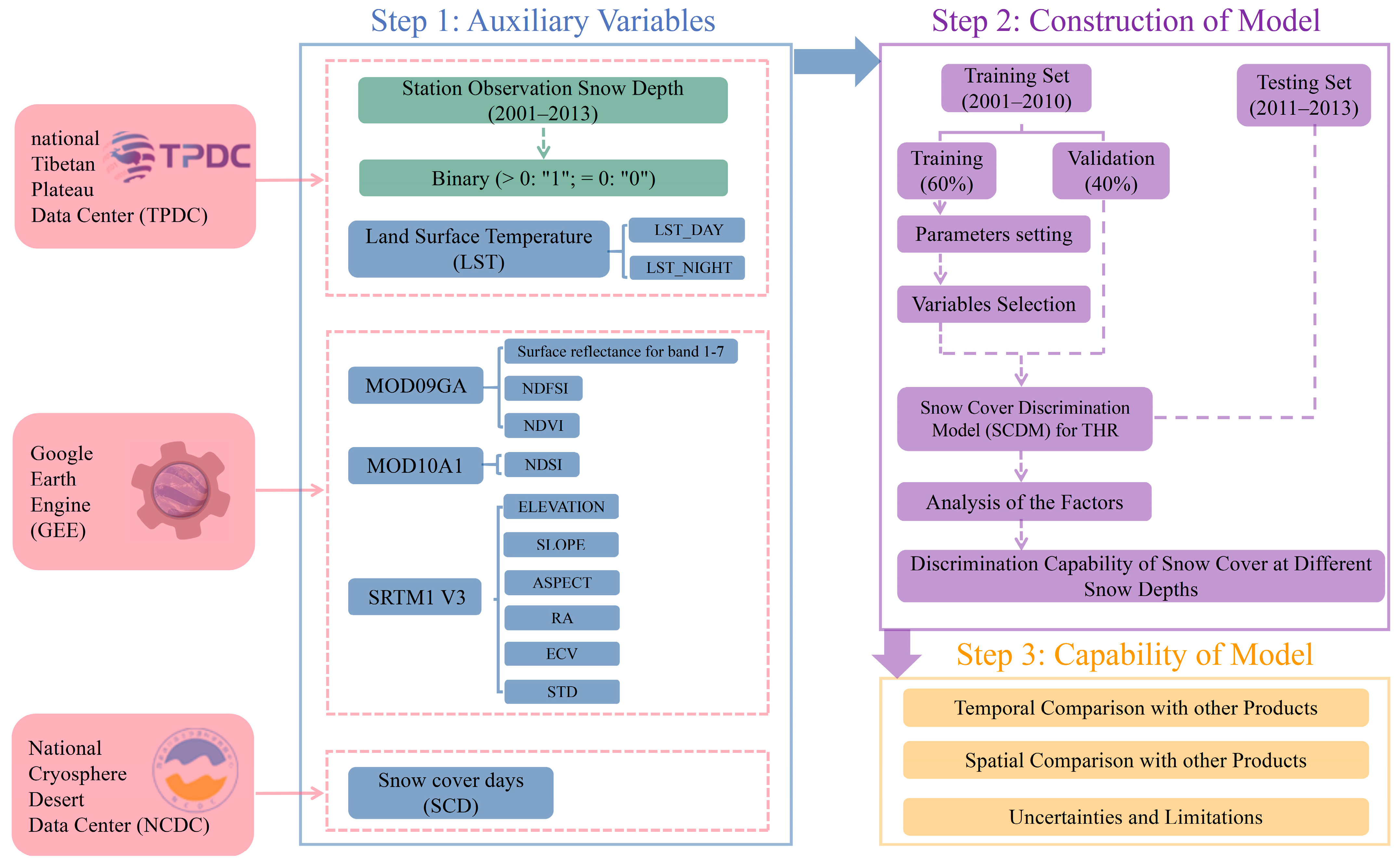
Figure 1. Flowchart.
Remotesensing 15 04644 g001
Figure 2. Study area overview: (a) Location of the THR. (b) Topographic distribution of the THR. (c) Land cover types in the THR. The points represent the average snow depth at each station during 2001–2013.The rectangular frames 1–8 represent 8 testing areas for evaluating the performance of the snow cover discrimination model (SCDM) at the local spatial scale.
Remotesensing 15 04644 g002
Figure 3. Model performance metrics with different values of (a) Ntree, (b) Mtry when Ntree = 1000, and (c) ratio when Ntree = 1000 and Mtry = 2. The blue vertical dot line in subfigure (c) represents the optimal ratio in pixel scale.
Remotesensing 15 04644 g003
Figure 4. (a) Importance ranking of factors of snow cover distribution and (bi) partial dependence relationships between snow cover distribution probability and factors.
Remotesensing 15 04644 g004
Figure 5. (a) Comparison of the snow cover discrimination results of the SCDM: SCDM excluding LST (E-LST), SCDM excluding NDVI (E-NDVI), and SCDM excluding both LST and NDVI (E-LST + NDVI). (b) Snow cover discrimination accuracy based on the NDSI dynamic threshold method and SCDM.
Remotesensing 15 04644 g005
Figure 6. (a) Comparison of four methods of discriminating snow cover samples with station observations during 2001–2013 (the “number of snow cover sample” refers to the sum of snow cover samples at a given time for all stations), and (b) correlation analysis between station observations and SCDM, SDML_Che, MODIS_Qiu, and MODIS_Hao.
Remotesensing 15 04644 g006
Figure 7. Comparison of snow cover discrimination results between the SCDM and other snow cover products within the study region (testing areas 1–4 in Figure 2) and outside the study region (testing areas 5–8 in Figure 2). The first column (a1h1) shows Landsat-7 ETM images, the second column (a2h2) shows the snow classification results based on the Landsat-7 ETM images, the third column (a3h3) shows the discrimination results of the SCDM, the fourth column (a4h4) shows the snow products produced by Qiu, and the fifth column (a5h5) shows the snow products produced by Hao.
Remotesensing 15 04644 g007
Figure 8. (a) Correlation between snow cover fraction (SCF) and the optimal ratio. (b) Recommended ratio values for snow cover discrimination in the THR based on different SCFs.
Remotesensing 15 04644 g008
Table 1. Potential indicators of factors affecting snow cover distribution in the THR.
Variable NameCodeUnitNote
Surface reflectance for band 1ref1nm620–670
Surface reflectance for band 2ref2841–876
Surface reflectance for band 3ref3459–479
Surface reflectance for band 4ref4545–565
Surface reflectance for band 5ref51230–1250
Surface reflectance for band 6ref61628–1652
Surface reflectance for band 7ref72105–2155
Normalized Difference Vegetation IndexNDVI
Normalized Difference Snow IndexNDSI
Normalized Difference Forest Snow IndexNDFSI
Land surface temperature in the dayLST_DAY°C
Land surface temperature in the nightLST_NIGHT°C
Snow cover daysSCDDay
SlopeSLOPE°
AspectASPECT°
ElevationELEVATIONm
Relief amplitudeRA
Elevation coefficient of variationECV
Terrain standard deviationSTD
Table 2. Performance of the SCDM.
Data SetAccuracyAUCKappaF1PrecisionRecall
Training set (2001–2010)0.99510.99400.94700.94960.96580.9339
Testing set (2011–2013)0.99080.98750.90630.91110.89660.9262
Unselected sites0.98420.90800.71440.72210.91860.5949
Shallow snow cover sample set (SD ≤ 2 cm)0.97980.87750.59250.60180.88610.4556
Disclaimer/Publisher’s Note: The statements, opinions and data contained in all publications are solely those of the individual author(s) and contributor(s) and not of MDPI and/or the editor(s). MDPI and/or the editor(s) disclaim responsibility for any injury to people or property resulting from any ideas, methods, instructions or products referred to in the content.