Article

A Downscaling–Merging Scheme for Monthly Precipitation Estimation with High Resolution Based on CBAM-ConvLSTM

1
State Key Laboratory of Water Resources Engineering and Management, Wuhan University, Wuhan 430072, China
2
Anhui Survey and Design Institute of Water Resources and Hydropower Co., Ltd., Hefei 230088, China
*
Author to whom correspondence should be addressed.
Remote Sens. 2023, 15(18), 4601; https://doi.org/10.3390/rs15184601
Submission received: 14 August 2023 / Revised: 13 September 2023 / Accepted: 15 September 2023 / Published: 19 September 2023
(This article belongs to the Special Issue Remote Sensing in Natural Resource and Water Environment II)

Abstract

:
Satellite products have mediocre performance in precipitation estimation, while rain gauges are incapable of describing continuous spatial precipitation distributions. To obtain spatially continuous and accurate precipitation data, this paper proposes a two-step scheme incorporating environmental variables, satellite precipitation estimations, and rain gauge observations for the calibration of satellite precipitation data. First, the GPM data are downscaled from 0.1° to 0.01° based on the seasonal RF models to minimize the spatial differences between the satellite estimations and the rain gauge observations. Secondly, the fusion model combining ConvLSTM and CBAM explores the spatiotemporal correlation of downscaled satellite precipitation data with environmental co-variables and ground-based observations to correct GPM precipitation. The integrated scheme (CBAM-ConvLSTM) is applied to acquire monthly precipitation at a spatial resolution of 0.01° over Hanjiang River Basin from 2014 to 2018. Comparative analyses of model-based satellite products with in situ observations show that model-based precipitation products have a high-resolution spatial distribution along with high accuracy, which combines the advantages of in situ observations and satellite products. Compared to the original GPM product, the evaluation metric values of the merged precipitation products all improved: the RMSE decreased by 31% while the CC increased from 0.55 to 0.69, the bias decreased from about 25% to less than 1.8%, and the MAE decreased by 27.8% while the KGE increased from 0.28 to 0.52. This two-step scheme provides an effective way to derive a high-resolution and accurate monthly precipitation product for humid regions.

1. Introduction

As a fundamental component of the terrestrial and hydrological cycle, precipitation is essential in hydrology, meteorology and ecology [1,2,3,4]. Owing to the spatiotemporal unevenness and variation of precipitation [5], obtaining accurate and high resolution precipitation data remains a great challenge. Furthermore, the quality of hydrological models is heavily reliant upon the quality of input data [6]. Thus, high-resolution and accurate precipitation data are necessary in many aspects, whereas traditional rainfall measurements mainly rely on rain gauges; the uneven distribution of gauges leads to difficulties in depicting precipitation distribution over areas with sparse rainfall stations.
Since the 1980s, satellite-based products are becoming an effective alternative for spatiotemporal precipitation estimates, facilitated by the boom in remote sensors and measurement technologies. With the different retrieval algorithms or satellite sources, there are some mainstream satellite precipitation products available around the world. For instance, the Tropical Precipitation Measurement Mission (TRMM) and the Global Precipitation Measurement Mission [7] (GPM, the successors of TRMM), developed by National Aeronautics and Space Administration (NASA) and Japanese Aerospace Exploration Agency (JAXA), provide [8,9] the TRMM Multi-satellite Precipitation Analysis (TMPA) [8,10] and Integrated Multi-satellite Retrievals (IMERG) [9] products, respectively. The [7] Global Precipitation Satellite Mapping (GSMaP) [10] is also a high-resolution global precipitation product developed by JAXA under the GPM program. In Europe, satellite-derived precipitation products from the Satellite Application Facility on Support to Operational Hydrology and Water Management (H-SAF) [11] are widely used. The Fengyu series satellite developed by China also provide precipitation products for East Asia [12]. However, certain limitations of satellite-based products have also been gradually made evident. For instance, most satellite-based precipitation products have large systematic biases and random errors compared to ground-based rainfall station observations [13]. Moreover, most satellite precipitation products have a relatively coarse spatial resolution and cannot be utilized directly for small-scale hydrological research [14,15]. Precipitation observations from rain gauge and remote sensing are complementary. Therefore, combining rain gauge observations with satellite precipitation products can produce spatiotemporal maps of precipitation with high resolution.
Over the past decade, calibrating satellite precipitation estimations with ground-based observations has become a prevalence to reduce the errors and improve the accuracy of satellite precipitation products. However, due to the large differences in spatial resolution between satellite precipitation data and in situ observations, the direct fusion of these two precipitation data has resulted in a bias near the boundary between the two continuous grids of satellite precipitation data [16]. In addition, several studies have stated that satellite products are often highly biased in time and space compared to in situ observations [17,18]. To address these issues, some studies have suggested that the satellite-based precipitation data need to be downscaled to match the scales of the ground observation sources before fusion [19]. A study has integrated three satellite-based products (GPM, CMORPH and GSMaP) with a high-density rainfall station network to create a highly accurate daily precipitation product [20]. Chen et al., (2020) [21] merged four downscaled satellite-based products with in situ observations based on the Geographically Weighted Ridge Regression (GWRR) method.
Traditional multi-source precipitation fusion methods are mainly based on mathematical concepts such as weighted averaging and regression to deal with the errors of precipitation products. These methods include probability matching methods [16], statistical bias correction [22], the kriging method [23], geo-graphically weighted regression (GWR) [24], etc. Nevertheless, the above methods are usually under restricted hypotheses and generally consider only spatial or temporal factors without incorporating both effects. In contrast, deep learning models are able to handle complicated nonlinear relations among variables without restricting mathematical hypotheses because of their great ability to learn and generalize. With the flourishing development and widespread use of machine learning, these algorithms have also been applied in precipitation downscaling and multiple sources merging. Among them, random forests (RF) can handle the complex non-linear relationships between variables because they are insensitive to covariance between variables and minimize the overfitting problem [25]. Thus, a random forest algorithm has great potential in downscaling satellite precipitation data. Shi et al., (2015) [26] applied the random forest model to monthly scale TRMM precipitation data and found that the downscaling results based on random forest achieved a higher accuracy than those based on linear regression methods and exponential regression methods. Jing et al., (2016) [27] spatially downscaled yearly TRMM (3B43 V7) precipitation data in the Tibetan Plateau region by RF and support vector machine (SVM), respectively, and found that the random forest-based downscaling results had better performance. A fusion model combining the Convolutional Neural Network (CNN) and the Long Short-Term Memory (LSTM) network for satellite and gauge precipitation outperformed the original TRMM daily products in China [28]. The fusion model used in this paper is based on the Convolutional LSTM network (ConvLSTM) proposed by Shi et al., (2015) [29]. The ability of ConvLSTM to capture both the temporal correlation of time-series data and the spatial distribution characteristics of data has been proved, and this network has been consequently used in rainfall nowcasting [30,31].
Moreover, the correction and analysis of precipitation data are still great challenges owing to the lack of robustness and stability of time series. A neural network extracts the information by convolutional operations, and each feature has a different influence in the neural network [32]. Therefore, introducing an attention mechanism in deep learning networks can simplify the model and speed up the computation. In the literature, the importance of attention has been studied and demonstrated [33,34,35]. Among the various attention mechanism modules that have been proposed, the Convolutional Block Attention Module (CBAM) [35] has been tested to achieve better results plugging at CNNs (Convolutional Neural Networks) than attentional mechanisms that focus only on channels [34]. Incorporating the strengths of the above models, a hybrid model integrating ConvLSTM and CBAM is applied to better implement the analysis and correction of satellite precipitation sequences.
The main objective of this study is to develop a downscaling–merging framework based on RF, ConvLSTM and CBAM and to generate high-resolution monthly precipitation data with high accuracy by merging satellite- and gauge-based data. To address these concerns, two steps are implemented: firstly, the GPM_3IMERGDF monthly precipitation is spatially downscaled based on an RF model. Secondly, downscaled GPM precipitation data are merged with in situ observations by the ConvLSTM network to acquire monthly high-resolution precipitation estimations. In addition, in order to emphasize the crucial features at different periods and locations on GPM images, a Convolutional Block Attention Module (CBAM) is placed at the ConvLSTM architectures. In conclusion, the validity of the downscaling–merging model is tested by comparing it with other comparative methods using merged GPM estimations and rain gauge observations.

2. Study Area and Data Source
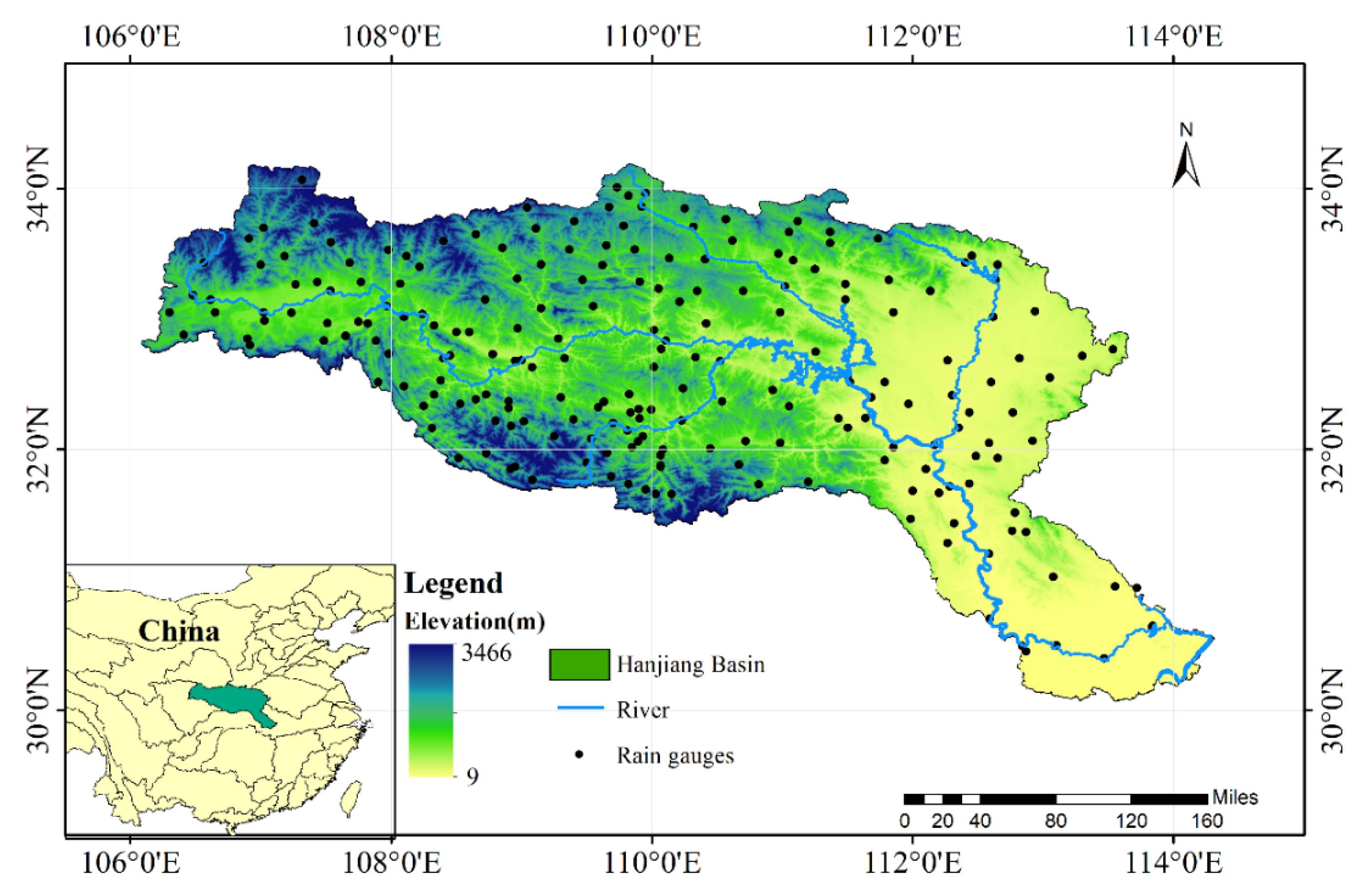
2.1. Study Area

The Hanjiang River, with a total length of 1532 km, is the largest tributary of the Yangtze River, flowing through five provinces: Shaanxi, Gansu, Sichuan, Henan and Hubei. As shown in Figure 1, the Hanjiang River Basin, with the area of 159,000 km2, is located in south of central China, at 30°4′~34°11′N and 106°5′~114°18′E [36]. The altitude of the river basin is ranging from 9 to 3466 m, lower in the southeastern region. The distribution of precipitation is strongly uneven, varying with longitude, latitude and altitude. The Hanjiang River Basin is in the region of the subtropical monsoon with a mild and humid climate. Precipitation in the basin is abundant: the annual average is about 870 mm, with above 3/4 falling from May to October, indicating a large inter-annual variation.

2.2. Datasets

The ground observation data used in this study were provided by a dense network of rain gauges in the Hanjiang River Basin, maintained by the Ministry of Water Resources. Daily precipitation from a total of 222 in situ gauges between March 2014 and February 2018 were retrieved from the hydrological yearbook of China. The distribution and location of the dense rain gauges is shown in Figure 1.
The V06 final IMERG daily precipitation product (GPM_3IMERGDF) with a spatial resolution of 0.1° × 0.1° is used in this study. The Global Precipitation Measurement (GPM) Mission is deployed by The National Aeronautics and Space Administration (NASA) and the Japan Aerospace and Exploration Agency (JAXA) in 2014 [7]. The level 3 merged product, Integrated Mulit-satellite Retrievals for GPM (IMERG), is the merging of GPM Microwave Imager (GMI) retrievals, partner radiometers and infrared (IR)-based observations with monthly surface precipitation. The GPM data are in netCDF format and contain mainly precipitation and spatiotemporal information related to the precipitation.
The Normalized Difference Vegetation Index (NDVI), the Digital Elevation Model (DEM) data and the Land Surface Temperature (LST) data are used for modelling the correlation between precipitation and environmental variables. The Moderate Resolution Imaging Spectroradiometer (MODIS) sensors on the Terra satellite provide monthly NDVI data at a spatial resolution of 1 km × 1 km. NDVI values generally below 0.0 in areas with coverage of water bodies, snowfield and deserts. To remove the effects of snow and water, the original monthly NDVI under 0.0 is regarded as missing measurements and interpolated using the moving window method. The night and day LST data derive from MOD11A2, which is developed by the NASA Land Processes Distributed Active Archive Center (LPDAAC). The LST data are at a temporal resolution of eight days and a spatial resolution of 1 km × 1 km. DEM data with a spatial resolution of 90 m are acquired from the Resource and Environment Science and Data Centre of the Chinese Academy of Sciences for mainland China, and the slope and aspect are calculated based on the DEM. All datasets involved in this study cover the period March 2014 to February 2018 and a brief description is available in Table 1.

3. Methodology

This section describes the downscaling–merging method developed as a two-step procedure (Figure 2): (1) spatial downscaling based on the RF model, and (2) satellite and gauge precipitation data fusion based on Convolutional LSTM and CBAM. The aim is to obtain satellite precipitation estimations with high spatial resolution and improved accuracy. Then, the evaluation method of merged precipitation data and the metrics used are presented.

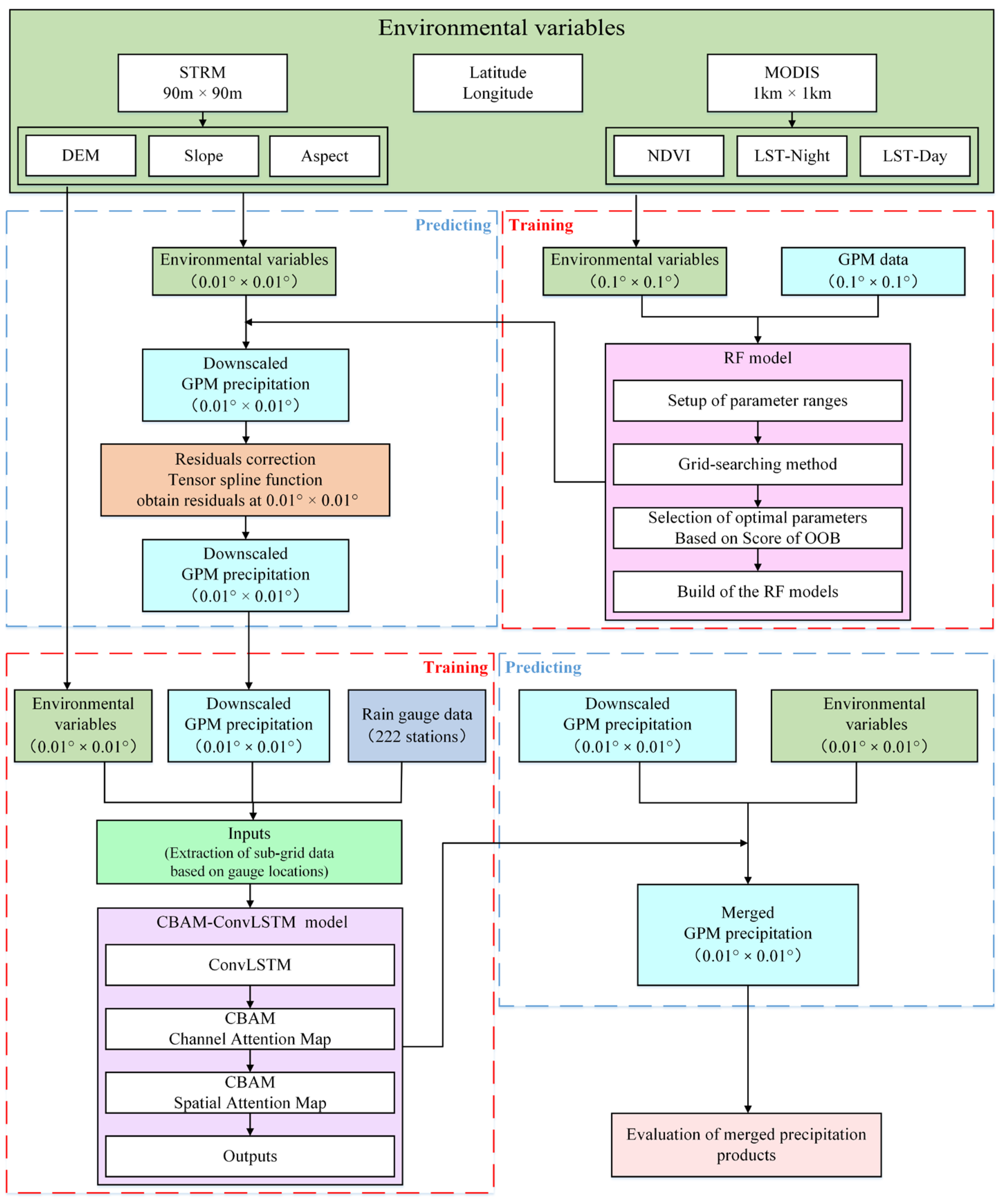
3.1. Downscaling of GPM Based on RF

Random forests (RFs), firstly proposed by Breiman (2001) [25], are ensemble learning algorithms based on decision trees. As ensemble classifiers, RFs are more robust than individual decision trees. The RF extracts multiple subsets from the original training dataset based on the Bootstrap Aggregating (Bagging) [37,38] approach and builds corresponding decision trees using covariate input for model training. The final predictions are determined by averaging outputs (for regression) or voting (for classification). The unselected samples (Out-of-bag, OOB) can be used to rank the importance of the covariates involved in the modelling [39]. Random forests can predict multiple factors and fit non-linear relationships, hence performing well in downscaling meteorological data such as precipitation and temperature [40,41].
Studies have pointed out that strong interactions exist among precipitation and environmental variables at both annual and monthly scales, whereas such interactions are lacking at the daily scale [27,42]. Therefore, four RF [43] models were developed to spatially downscale the GPM data at different seasons. The seasonal GPM precipitation data at spatial resolution of 0.01° × 0.01° were subsequently decomposed to a monthly scale. The main steps are as follows:
  • Data processing: To maintain consistency with the resolution of GPM precipitation data, selected environmental variables (nighttime and daytime LST, NDVI, topographic data including DEM, slope and aspect) were resampled to a spatial resolution of 0.01° × 0.01° and 0.1° × 0.1° by bilinear interpolation. Based on the climatic characteristics of the Hanjiang River Basin, twelve months were equally divided into four seasons, of which March is the beginning of spring. Precipitation (GPM and in situ observation daily data) and environmental variables (nighttime and daytime LST, NDVI) were accumulated into seasonal data.
  • Downscaling model construction: Separated RF models were developed for different seasons and were, respectively, trained by seasonal GPM precipitation, geographical location (latitude and longitude), NDVI, LST, and the terrain feature dataset (DEM, slope and aspect) at 0.1° × 0.1° spatial resolution. The 0.01° × 0.01° environmental variables were fed into the developed regression model to obtain seasonal GPM precipitation with 0.01° × 0.01°.
  • Residuals’ correction: Model residuals were calculated and then interpolated using a tensor spline function to obtain residuals at 0.01° × 0.01°. The residuals were consequently used to correct for downscaled precipitation results.
  • Seasonal GPM precipitation decomposition: The high-spatial-resolution GPM precipitation was decomposed based on the ratio of month to season data, with the hypothesis that the ratio remains constant [42].

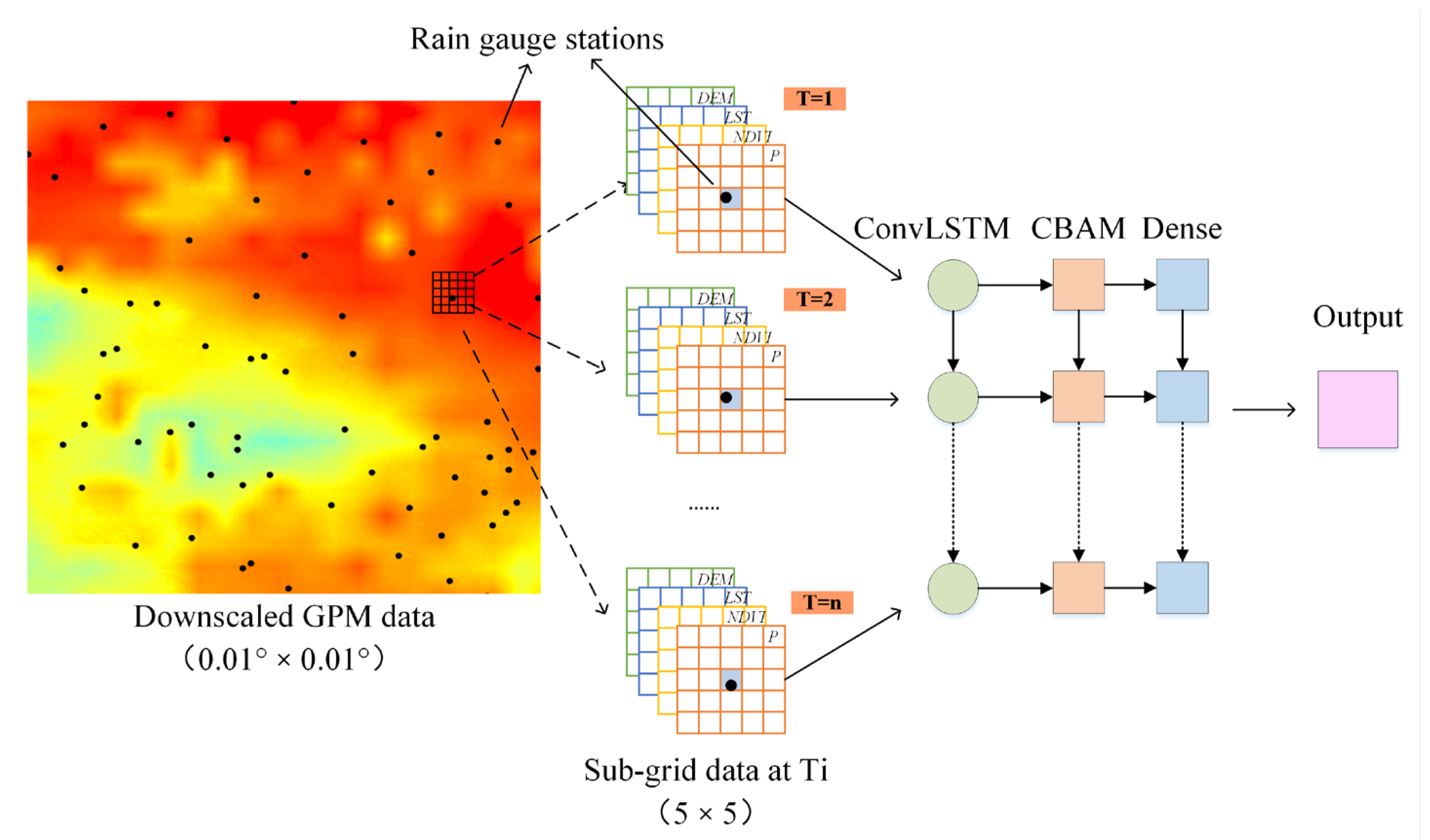
3.2. Merging of GPM and Gauge Observations Based on ConvLSTM and CBAM

ConvLSTM (Convolutional LSTM) [29] is a hybrid variant of the LSTM. Since the input to an LSTM is a one-dimensional tensor, it cannot capture spatial features. ConvLSTM, on the other hand, uses convolutional operators rather than matrix multiplication to input states and state-to-state transitions. ConvLSTM can therefore not only obtain temporal relationships but also extract spatially correlated features such as convolutional layers, and has been shown to be effective in many applications [44,45,46].
Four structures are specific to ConvLSTM: The cell state is used to store the accumulation of past information. The forget gate, f, determines how much of the cell state at the previous moment is retained to the current time. The input gate, i, determines how much information of the network input is saved to the cell state at the current time, and the output gate, o, determines how much information the cell state outputs. H, C and X represent the hidden state, and the cell output and inputs of each timestamp, separately. The main equations for ConvLSTM are as follows:
i t = σ ( W x i * X t + W h i * H t 1 + W c i C t 1 + b i ) f t = σ ( W x f * X t + W h f * H t 1 + W c f C t 1 + b f ) C t = f t C t 1 + i t tanh ( W x c * X t + W h c * H t 1 + b c ) o t = σ ( W x o * X t + W h o * H t 1 + W c o C t 1 + b o ) H t = o t tanh ( C t )
where and represent the convolution operation and the Hadamard product, respectively. σ is the sigmoid activation function.
The Convolutional Block Attention Module (CBAM) [35] is a feed-forward convolutional neural network attention module to focus on important features and suppress unnecessary ones. CBAM sequentially applies channel and spatial attention modules. CBAM calculates the weight map of an intermediary feature map given by a ConvLSTM network in the channel and spatial dimensions. The attention map is then multiplied by the input feature map to refine the adaptive features. The CBAM process can be summarized as follows:
F = M C ( F ) F F = M S ( F ) F
where represents the multiplication operation. MC(F) and MS(F′) are the channel attention map and spatial attention map separately. F, F′ and F″ are the feature map at input, after channel attention and output correspondingly.
Average-pooling and max-pooling are applied to spatial and channel feature maps, respectively, and the resulting descriptors are forwarded into a multi-layer perceptron (MLP) with a hidden layer and then concatenated to the convolution layer. The channel attention and spatial attention are computed as
M C ( F ) = σ ( M L P ( A v g P o o l ( F ) ) + M L P ( M a x P o o l ( F ) ) )
M S ( F ) = σ ( f 7 × 7 ( [ A v g P o o l ( F ) ; M a x P o o l ( F ) ] ) )
where f7×7 is the convolution operation and σ is sigmoid activation function.
A schematic diagram of the satellite sub-grid extraction method is shown in Figure 3. A CBAM-ConvLSTM network was used to build the GPM and gauge data fusion model. The structure and hyper-parameter design of the CBAM-ConvLSTM deep fusion model are shown in Figure 4a:
  • All input datasets including in situ precipitation observations, downscaled GPM data and surface environmental variables (NDVI, LST, DEM) were normalized.
  • The 5 × 5 sub-grids were extracted from the satellite grid to represent the spatial distribution of precipitation at the current rain gauge, centered on the nearest grid of 222 rain gauges.
  • The training data corresponding to the satellite grid data and ground observation data in time and space were established. The image size of input variables is 5 × 5 × 5 × 5 (image size is 5 × 5, number of channels is 5). A time step (T) of 5 and a kernel of 3 × 3 were chosen. The epoch and learning rate of the established CBAM-ConvLSTM network were 100 and 0.001, respectively. The number of units in ConvLSTM was set to 8. To avoid overfitting, a regularization method (Dropout, parameter set to 0.25) was applied. Dense represents a fully connected layer, followed by the number of convolution kernels, with ‘elu’ as the activation function. The fused precipitation over the entire study area was obtained by feeding grid data into the fusion model to obtain precipitation at each grid point location.
  • The model performance was evaluated using 10-fold cross-validation, dividing the 222 rain gauges into 10 parts, each of which will be tested. The mean of all tested rain gauges was used as the assessment result.

3.3. Evaluation Criteria

To qualitatively assess the performance of downscaled and CBAM-ConvLSTM-based fusion products against in situ observations, all datasets from 222 rain gauges were partitioned into training and testing datasets on a ratio of 9:1 by 10-fold cross-validation. The model performance at each rain gauge station was assessed by the average of ten training models. The metrics used to calculate the accuracy of precipitation estimations include ME, r, Bias, KGE [47], RMSE and MAE. The equations and the optimums of evaluation metrics are expressed in Table 2.

4. Results

4.1. Performance of RF-Based Downscaling Models

The predictive performance of the downscaled models is evaluated using the 10-fold cross-validation method. CC, RMSE and ME of the original GPM data at 0.1° × 0.1° spatial resolution with precipitation predicted by the RF models during 2014 to 2017 were calculated (Table 3). CC values are all greater than 0.99, indicating that the model predicted data fit well with the original GPM data. Most of the RMSEs are less than 30 mm, and the ME are less than 6 mm. Moreover, the values of ME are all greater than zero, indicating that models have slightly overestimated the precipitation values. Overall, RF models show strong prediction ability on independent datasets and the environmental variables are greatly associated with precipitation. Therefore, downscaling regression models constructed based on the RF can be applied to the spatial downscaling of GPM precipitation data.

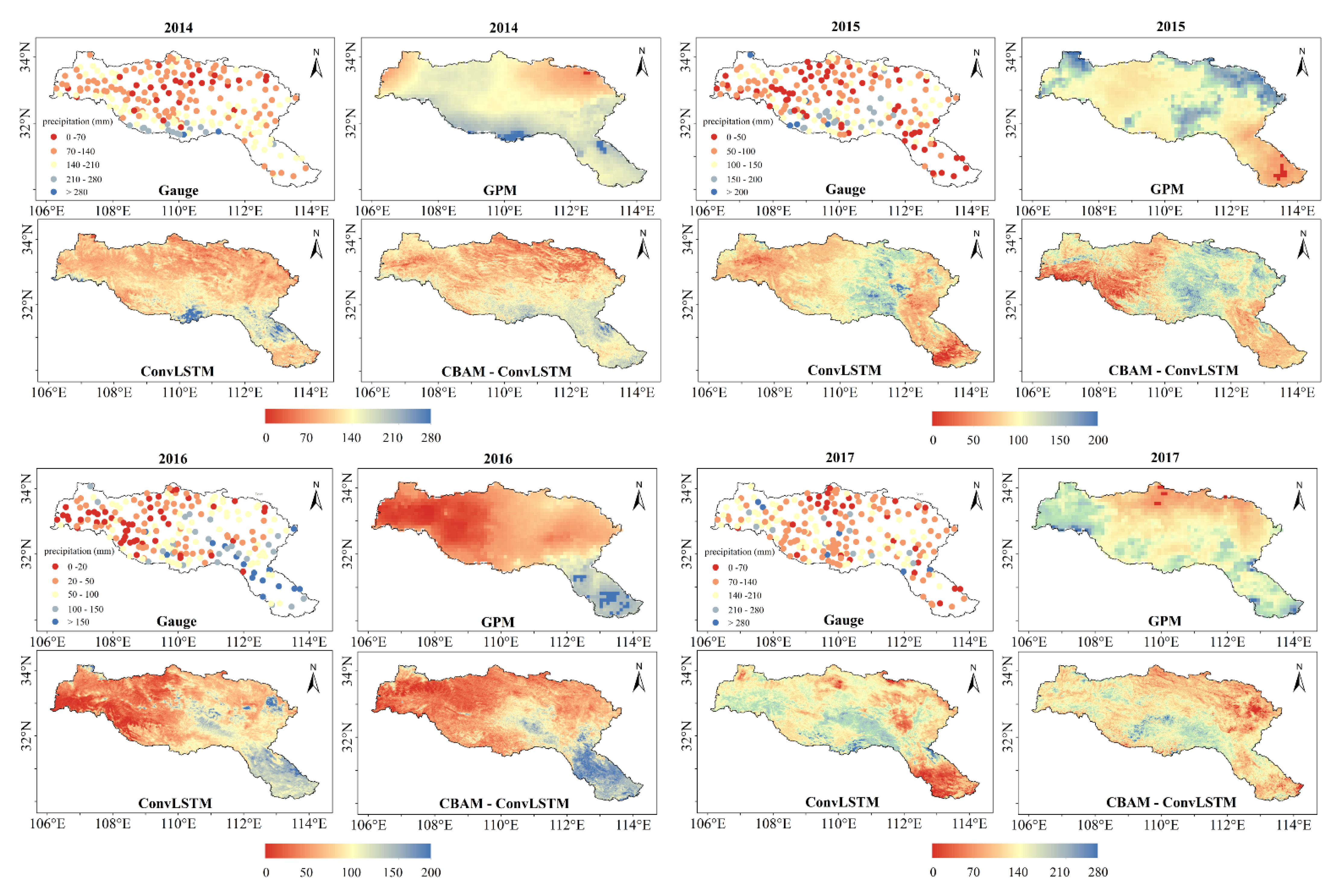
4.2. Performances of Merged Precipitation Products

The correlation of GPM and three model-based (RF, ConvLSTM and CBAM-ConvLSTM) precipitation estimations versus in situ observations on a monthly scale is shown in Figure 5. The correlation coefficients between GPM-based precipitation estimates (GPM, RF, ConvLSTM and CBAM-ConvLSTM) and the rain gauge data range from 0.69 to 0.85, suggesting a relatively strong correlation between four GPM-based products and rain gauge data, while both GPM and model-based products underestimated precipitation. As seen in Figure 5a,b, the distribution of original GPM and RF data is similar and more discrete at the points of high precipitation, which indicates that higher precipitation leads to higher bias. In addition, the RF model did not provide a significant improvement in its accuracy during downscaling. Compared with RF-downscaled GPM, the accuracy of precipitation estimations is improved after being merged with the in situ observations. The performance of CBAM-ConvLSTM was the optimum among the four GPM-based products with the closest points to the 1:1 line.
The spatial distribution of original GPM and downscaled–merged precipitation products (ConvLSTM and CBAM-ConvLSTM) for the August of each year (2014–2018) is shown in Figure 6. As can be seen, the spatial consistency of the GPM is poor due to its low resolution and the lack of continuity transitions in precipitation data between different regions. The fused GPM product maintains the spatial distribution of the original GPM data while greatly enhancing details of precipitation maps. The distribution of satellite precipitation data is more continuous and the transition between rainy and no-rain areas is smoother. This improvement is especially obvious for the uneven precipitation distribution regions. When fused with rain gauge data, the GPM monthly precipitation is significantly corrected in two aspects. Foremost, for almost all precipitations, the original GPM tends to underestimate the precipitation, and the fusion process calibrated the GPM monthly precipitation to some extent. For example, for August 2014 precipitation, the GPM estimations underestimated precipitation in the north and east regions of Hanjiang River Basin, and the fusion process contributed to a notable increase in precipitation in these parts of the study area. Second, the fusion results also illustrate the detail of rainfall distribution. For instance, in August 2016, the original GPM showed almost no precipitation in the central region of the Hanjiang River Basin, whereas the fused data showed precipitation covering the area. In both model-based data, CBAM-ConvLSTM outperformed ConvLSTM. ConvLSTM showed underestimation in the western part of the Hanjiang River Basin in both August 2015 and August 2017, and showed occasional overestimated precipitation grids in the southern (August 2014) and northeastern (August 2016) parts of the study area.

4.3. Accuracy Assessment of Merged Precipitation Product

In order to assess the performance of the models, quantitative evaluation of the monthly original GPM data and three model-based GPMs involved in the downscaling–merging procedure against the 222-rain-gauge datasets is presented in Table 4. Among the statistics of four GPMs, mean value of CC, bias, KGE, RMSE and MAE for CBAM-ConvLSTM is 0.69, 1.79%, 0.52, 26.30 and 20.37, respectively, testifying to the best performance of the CBAM-ConvLSTM model followed by ConvLSTM, GPM and RF. Similar quantitative results of the RF and GPM reveal that the accuracy of the downscaled GPM was substantially similar to that of original GPM during the entire study period, which is in agreement with the results shown in Figure 5. In general, ensemble merging models including ConvLSTM and CBAM-ConvLSTM outperform GPM and RF given the increases of KGE and CC as well as the decreases of bias, MAE and RMSE. Furthermore, CBAM-ConvLSTM reduced by 12.1% and 13.9% in MAE and RMSE of ConvLSTM, respectively, while increasing its CC by 11.3%. Hence, CBAM has led to a moderate improvement compared to the ConvLSTM, which is due to the fact that the attention module captured important information from the feature map.
Figure 7 illustrates the model performance of RF, ConvLSTM and CBAM-ConvLSTM at relative bias, CC, KGE and RMSE at seasonal and monthly scale. Boxplots of the original GPM metrics are also shown for comparison. In the monthly scale, the performance of CBAM-ConvLSTM is optimal with the highest median KGE and CC values among four products, indicating that GPM merging with environmental co-variables and rain gauge data develops the performance of GPM. Especially in summer seasons, when precipitation occurs most frequently, the CBAM-ConvLSTM is superior to other precipitation products. Additionally, the median values of metrics and dispersion of the boxplots for GPM and RF are similar at both monthly and seasonal scales, emphasizing that the RF model captures the major information of GPM precipitation during downscaling. However, the boxplots of CBAM-ConvLSTM in winter show a wider dispersion and a relative low KGE value, whereas RMSE is smaller. This unstable performance of the merging model is associated with the high bias of original GPM and the lack of precipitation data for the training period in winter. On the other hand, NDVI contributes less to the model due to the lower vegetation cover in winter. Despite the weak correlations and high bias between merged products and in situ observations in winter, the overall performance of ensemble merging models based on deep learning is doing better than the original and downscaled GPM. Moreover, three model-based products capture the temporal variability of precipitation.
In addition, Taylor plots were shown to visually compare in situ observations, original GPM precipitation estimates, downscaled GPM precipitation estimates, and downscaled–fused precipitation estimates at a monthly scale (Figure 8). In the Taylor diagram, a better performance is indicated if the point representing monthly precipitation estimates is closer to the point representing gauge observations. Figure 8 confirms that the accuracy of RF-based downscaled GPM and original GPM were similar, while the integrated fusion scheme based on RF and CBAM-ConvLSTM decreased the error of monthly precipitation. Significantly, the standard deviation of ConvLSTM and CBAM-ConvLSTM has slightly decreased compared to the in situ observations, which is in line with the results of Chen et al., (2020) [19]. This decrease is attributed to the discontinuous spatial distribution of the precipitation data provided by the rain gauge observations, whereas the precipitation distribution of the fused GPM data is spatially continuous.
Three monthly precipitation products (GPM, ConvLSTM and CBAM-ConvLSTM) were further compared on their capability of capturing the variations of precipitation at rain gauge locations. Figure 9 shows such a comparison for CC, MAE and RMSE at the rain gauge locations. As shown in Figure 9, most of the CC-values ranged from 0.6 to 0.8, especially in the upper reaches of the Hanjiang River Basin, where the CC of most locations are greater than 0.7. This indicates that the GPM data are in relatively strong correlations with the ground based observations. After fusion with the in situ observations, the CC of the ConvLSTM are more than 0.75 for most of the locations, and the CC of the CBAM-ConvLSTM are greater than 0.9 at most of stations, and these locations are mainly distributed in the upper Hanjiang River Basin. Compared with CBAM-ConvLSTM, the MAEs of GPM and ConvLSTM are higher than 20 mm at most locations. In contrast, the MAE of CBAM-ConvLSTM decreased significantly and was less than 20 mm at most locations. Additionally, there are obvious regional variations in the distribution of the MAE values, and the areas with higher values are mainly located in the southeastern part of the Hanjiang River Basin, which is also an area of lower elevation. The spatial pattern of RMSE is similar to that of MAE, with the RMSE values of GPM and ConvLSTM being larger than 25 mm at most locations. Meanwhile, CBAM-ConvLSTM shows a significant decrease in RMSE at almost all locations, with those values less than 25 mm at most locations. As expected, CBAM-ConvLSTM has better performance than GPM and ConvLSTM: CBAM-ConvLSTM significantly increases CC and decreases MAE and RMSE compared to GPM, indicating that the consistency between the model-based precipitation data and the rain gauge data is significantly improved while the error is reduced.

5. Discussion

Overall, the diversity of topography and precipitation types in the study area provides a basis for a comprehensive evaluation of the proposed downscaling–merging scheme. Three crucial factors for the downscaling–merging modeling are the choice of time scale, environmental variable selection, and methods of accessing the correlation among satellite, gauge precipitation and environmental variables. First, choosing an appropriate time scale is a necessary precondition for modeling. Typically, the interaction between precipitation and environmental variables is not strong at the daily scale. Hence, some studies have spatially downscaled precipitation data from a monthly scale [48], but they are limited to specific months, e.g., the month when vegetation grows. This is explained by the fact that the strong connection between precipitation and environmental variables exists only during these months. A 2- or 3-month delay in vegetation response to precipitation has been reported in some findings, suggesting that seasonal time scale analysis can explain the effect of vegetation on precipitation. Second, unlike some spatial downscaling studies, this study introduces latitude and longitude as supporting co-variables, and comparative analyses show that the introduction of geographic location significantly enhances the ability of RF model to explain precipitation variability. A similar situation was found by Bryan et al., (2002) [49] and Price et al., (2000) [50], who pointed out the important relationship between precipitation and geographic location. In addition, terrain interacts with precipitation in a sophisticated way. Although topography tends not to disturb precipitation on plains with small spatial differences in elevation [51], mountains not only have a lifting effect on airflow, but also have a blocking effect on airflow. Land surface temperature has a significant effect on precipitation, but the relative importance of daytime and nighttime LST on precipitation varies, with the importance of LST at night being relatively high [52]. Moreover, nighttime LST also has a greater influence on precipitation than other land surface environmental variables in humid regions [27]. Therefore, both LST at night and day are used for modelling. Other environmental variables, including atmospheric variables or land use, also have an impact on precipitation. As discussed above, downscaling of low-resolution satellite precipitation data relies on high-resolution environmental variables, and the calibration of satellite precipitation with rain gauge data also relies on environmental variables with strong correlations. However, there are fewer high-resolution environmental variables that are reliable in practical studies. In addition, the models developed are inherently spatially variable and therefore cannot use categorical variables (e.g., data such as vegetation coverage and land use). Under these considerations, four environmental variables are used to construct downscaling and fusion models. The accuracy assessment results suggest that the accuracy of the model based GPM data is well maintained before and after the downscaling–merging process, indicating that the environmental co-variables selected for modeling are rational.
The downscaling of GPM precipitation data by RF-based downscaling model provides an effective solution to the issue of deviation between the discontinuous precipitation background field (rain gauge data) and satellite grid data [16]. It is observed from the results that the accuracy of downscaled precipitation data through RF model was slightly improved compared with the GPM product. The satellite precipitation data distribution is more continuous due to a better spatial scale match between downscaled GPM data and rain gauge data, and the downscaling process has a certain smoothing effect. Therefore, the RF models used to downscale the GPM precipitation data alleviates the problem of boundary bias, and is conducive to the production of high-resolution precipitation distribution maps, which plays a role in improving the accuracy of the fusion results.
Many studies have applied GWR and Kriging or their improved methods [21,24,53,54] to implement the fusion of satellite precipitation estimations and in situ observations. Different from previous studies, this study introduces ConvLSTM to construct a fusion scheme along with a machine learning algorithm (RF) in the downscaling process. In particular, with the introduction of the CBAM module, the accuracy of the fusion model is improved on both spatial and temporal scales and the results show that the accuracy of merged precipitation data at the monthly scale is significantly improved. Above all, the proposed machine learning-based downscaling–merging method is considered valuable and effective.

6. Conclusions

A downscaling–merging scheme is proposed to produce a high-quality monthly precipitation dataset with a spatial resolution of 0.01° in the Hanjiang River Basin. This method involves two steps: First, downscaling is performed with RF models. Subsequently, correcting the GPM data by merging the GPM data and in situ observations with CBAM-ConvLSTM. The main findings are as follows:
  • The downscaling algorithm based on RF models significantly refined the spatial resolution of GPM precipitation and maintains a moderate accuracy. Due to the improved spatial resolution, the spatial mismatch between downscaled precipitation data and rain gauge data is reduced, which improves its consistency with in situ observations. This reduces the error and provides a good basis for subsequent precipitation data fusion.
  • Considering the spatiotemporal relation between ground-based observations and satellite-based precipitation, a fusion model introducing ConvLSTM for merged precipitation data was proposed. The accuracy of the fused GPM is evaluated and the assessment results reveal that the accuracy of GPM is significantly improved after GPM data are fused with in situ observations. Compared with the original GPM, RMSE and MAE of the fused precipitation products were down by 19.9% and 17.9%, respectively. The bias was reduced to within 6%, and the CC and KGE were improved from 0.55 and 0.28 to 0.62 and 0.42, respectively.
  • The performance of the fused precipitation product was further enhanced with the introduction of the CBAM module. Compared to the original GPM, the RMSE of the fused precipitation product with the addition of the attention mechanism were reduced by 31% and the MAE of those decreased by 27.8%, respectively. Compared with ConvLSTM, the bias was reduced to within 2%, and the CC increased to 0.69 and the KGE rose to 0.52.
  • The downscaling step mitigates the bias problem caused by discontinuous precipitation background fields and provides the foundation for the fusion step. The monthly precipitation products achieved by the scheme maintained the original spatial information of the satellite data and significantly refined the spatial detail, portraying a continuous and accurate distribution of the satellite precipitation data. The improvement was particularly noticeable for areas of uneven precipitation distribution.
Adequate quality and high-resolution precipitation data are very meaningful for hydrological as well as meteorological analysis. Because of their characteristics, satellite-based products capture the cyclical patterns and regional distribution of precipitation. They provide a distribution map of precipitation, but are less accurate than rain gauge data. In this study, the vegetation index, topography, geographic location and surface temperature were taken as the main factors affecting precipitation, and a downscaling–fusion regression model was constructed. However, other factors including density of rain gauges and atmospheric circulation also have impact on precipitation, and according to the type of precipitation and the associated physical processes, other covariates can be considered in merging process for further study.

Author Contributions

Conceptualization, B.T., X.Y. and H.C.; methodology, B.T. and X.Y.; validation, B.T. and S.S.; formal analysis, B.T. and X.Y.; investigation, B.T., S.S. and K.L.; resources, H.C.; data curation, X.Y. and K.L.; writing—original draft preparation, B.T.; writing—review and editing, H.C.; visualization, B.T.; supervision, H.C.; funding acquisition, H.C. All authors have read and agreed to the published version of the manuscript.

Funding

This research was funded by the National Key Research and Development Program of China, grant number 2022YFC3002701.

Data Availability Statement

All data that support the findings of this study are included within the article. The rain gauge data used in this study are confidential.

Acknowledgments

The numerical calculations in this paper have been performed on the supercomputing system in the Supercomputing Centre of Wuhan University. The GPM (IMERG V06) Final Run data were provided by NASA, which develop and compute the IMERG V06 as a contribution to GPM, and archived at the NASA GES DISC.

Conflicts of Interest

The authors declare no conflict of interest.

References

  1. Del Jesus, M.; Rinaldo, A.; Rodríguez-Iturbe, I. Point rainfall statistics for ecohydrological analyses derived from satellite integrated rainfall measurements. Water Resour. Res. 2015, 51, 2974–2985. [Google Scholar] [CrossRef]
  2. Baez-Villanueva, O.M.; Zambrano-Bigiarini, M.; Beck, H.E.; McNamara, I.; Ribbe, L.; Nauditt, A.; Birkel, C.; Verbist, K.; Giraldo-Osorio, J.D.; Thinh, N.X. RF-MEP: A novel Random Forest method for merging gridded precipitation products and ground-based measurements. Remote Sens. Environ. 2020, 239, 111606. [Google Scholar] [CrossRef]
  3. Long, Y.P.; Zhang, Y.N.; Ma, Q.M. A Merging Framework for Rainfall Estimation at High Spatiotemporal Resolution for Distributed Hydrological Modeling in a Data-Scarce Area. Remote Sens. 2016, 8, 599. [Google Scholar] [CrossRef]
  4. Song, Y.Q.; Liu, H.N.; Wang, X.Y.; Zhang, N.; Sun, J.N. Numerical simulation of the impact of urban non-uniformity on precipitation. Adv. Atmos. Sci. 2016, 33, 783–793. [Google Scholar] [CrossRef]
  5. Ibarra-Berastegi, G.; Saenz, J.; Ezcurra, A.; Elias, A.; Argandona, J.D.; Errasti, I. Downscaling of surface moisture flux and precipitation in the Ebro Valley (Spain) using analogues and analogues followed by random forests and multiple linear regression. Hydrol. Earth Syst. Sci. 2011, 15, 1895–1907. [Google Scholar] [CrossRef]
  6. Kyriakidis, P.C.; Miller, N.L.; Kim, J. Uncertainty Propagation of Regional Climate Model Precipitation Forecasts to Hydrologic Impact Assessment. J. Hydrometeorol. 2001, 2, 140–160. [Google Scholar] [CrossRef]
  7. Hou, A.Y.; Kakar, R.K.; Neeck, S.; Azarbarzin, A.A.; Kummerow, C.D.; Kojima, M.; Oki, R.; Nakamura, K.; Iguchi, T. The Global Precipitation Measurement Mission. Bull. Am. Meteorol. Soc. 2014, 95, 701–722. [Google Scholar] [CrossRef]
  8. Huffman, G.J.; Bolvin, D.T.; Nelkin, E.J.; Wolff, D.B.; Adler, R.F.; Gu, G.; Hong, Y.; Bowman, K.P.; Stocker, E.F. The TRMM Multisatellite Precipitation Analysis (TMPA): Quasi-Global, Multiyear, Combined-Sensor Precipitation Estimates at Fine Scales. J. Hydrometeorol. 2007, 8, 38–55. [Google Scholar] [CrossRef]
  9. Tan, J.; Huffman, G.J.; Bolvin, D.T.; Nelkin, E.J. IMERG V06: Changes to the Morphing Algorithm. J. Atmos. Ocean. Technol. 2019, 36, 2471–2482. [Google Scholar] [CrossRef]
  10. Kubota, T.; Shige, S.; Hashizurne, H.; Aonashi, K.; Takahashi, N.; Seto, S.; Hirose, M.; Takayabu, Y.N.; Ushio, T.; Nakagawa, K.; et al. Global precipitation map using satellite-borne microwave radiometers by the GSMaP project: Production and validation. IEEE Trans. Geosci. Remote Sens. 2007, 45, 2259–2275. [Google Scholar] [CrossRef]
  11. Mugnai, A.; Casella, D.; Cattani, E.; Dietrich, S.; Laviola, S.; Levizzani, V.; Panegrossi, G.; Petracca, M.; Sanò, P.; Di Paola, F.; et al. Precipitation products from the hydrology SAF. Nat. Hazards Earth Syst. Sci. 2013, 13, 1959–1981. [Google Scholar] [CrossRef]
  12. Wu, H.; Yong, B.; Shen, Z. Research on the Monitoring Ability of Fengyun-Based Quantitative Precipitation Estimates for Capturing Heavy Precipitation: A Case Study of the “7·20” Rainstorm in Henan Province, China. Remote Sens. 2023, 15, 2726. [Google Scholar] [CrossRef]
  13. Shen, Y.; Xiong, A.; Wang, Y.; Xie, P. Performance of high-resolution satellite precipitation products over China. J. Geophys. Res. Atmos. 2010, 115, D02114. [Google Scholar] [CrossRef]
  14. Skofronick-Jackson, G.; Petersen, W.A.; Berg, W.; Kidd, C.; Stocker, E.F.; Kirschbaum, D.B.; Kakar, R.; Braun, S.A.; Huffman, G.J.; Iguchi, T.; et al. The Global Precipitation Measurement (GPM) Mission for Science and Society. Bull. Am. Meteorol. Soc. 2017, 98, 1679–1695. [Google Scholar] [CrossRef] [PubMed]
  15. Atkinson, P.M. Downscaling in remote sensing. Int. J. Appl. Earth Obs. Geoinf. 2013, 22, 106–114. [Google Scholar] [CrossRef]
  16. Li, M.; Shao, Q. An improved statistical approach to merge satellite rainfall estimates and raingauge data. J. Hydrol. 2010, 385, 51–64. [Google Scholar] [CrossRef]
  17. Hu, Q.; Yang, D.; Li, Z.; Mishra, A.K.; Wang, Y.; Yang, H. Multi-scale evaluation of six high-resolution satellite monthly rainfall estimates over a humid region in China with dense rain gauges. Int. J. Remote Sens. 2014, 35, 1272–1294. [Google Scholar] [CrossRef]
  18. Hong, Y.; Gochis, D.; Cheng, J.-T.; Hsu, K.-L.; Sorooshian, S. Evaluation of PERSIANN-CCS Rainfall Measurement Using the NAME Event Rain Gauge Network. J. Hydrometeorol. 2007, 8, 469–482. [Google Scholar] [CrossRef]
  19. Duan, Z.; Bastiaanssen, W.G.M. First results from Version 7 TRMM 3B43 precipitation product in combination with a new downscaling–calibration procedure. Remote Sens. Environ. 2013, 131, 1–13. [Google Scholar] [CrossRef]
  20. Li, K.; Tian, F.; Khan, M.Y.A.; Xu, R.; He, Z.; Yang, L.; Lu, H.; Ma, Y. A high-accuracy rainfall dataset by merging multiple satellites and dense gauges over the southern Tibetan Plateau for 2014–2019 warm seasons. Earth Syst. Sci. Data 2021, 13, 5455–5467. [Google Scholar] [CrossRef]
  21. Chen, S.L.; Xiong, L.H.; Ma, Q.M.; Kim, J.S.; Chen, J.; Xu, C.Y. Improving daily spatial precipitation estimates by merging gauge observation with multiple satellite-based precipitation products based on the geographically weighted ridge regression method. J. Hydrol. 2020, 589, 125156. [Google Scholar] [CrossRef]
  22. Beck, H.E.; Wood, E.F.; Pan, M.; Fisher, C.K.; Miralles, D.G.; van Dijk, A.I.J.M.; McVicar, T.R.; Adler, R.F. MSWEP V2 Global 3-Hourly 0.1 degrees Precipitation: Methodology and Quantitative Assessment. Bull. Am. Meteorol. Soc. 2019, 100, 473–502. [Google Scholar] [CrossRef]
  23. Manz, B.; Buytaert, W.; Zulkafli, Z.; Lavado, W.; Willems, B.; Robles, L.A.; Rodriguez-Sanchez, J.P. High-resolution satellite-gauge merged precipitation climatologies of the Tropical Andes. J. Geophys. Res.-Atmos. 2016, 121, 1190–1207. [Google Scholar] [CrossRef]
  24. Chao, L.; Zhang, K.; Li, Z.; Zhu, Y.; Wang, J.; Yu, Z. Geographically weighted regression based methods for merging satellite and gauge precipitation. J. Hydrol. 2018, 558, 275–289. [Google Scholar] [CrossRef]
  25. Breiman, L. Random Forests. Mach. Learn. 2001, 45, 5–32. [Google Scholar] [CrossRef]
  26. Shi, Y.L.; Song, L.; Xia, Z.; Lin, Y.R.; Myneni, R.B.; Choi, S.H.; Wang, L.; Ni, X.L.; Lao, C.L.; Yang, F.K. Mapping Annual Precipitation across Mainland China in the Period 2001–2010 from TRMM3B43 Product Using Spatial Downscaling Approach. Remote Sens. 2015, 7, 5849–5878. [Google Scholar] [CrossRef]
  27. Jing, W.L.; Yang, Y.P.; Yue, X.F.; Zhao, X.D. A Spatial Downscaling Algorithm for Satellite-Based Precipitation over the Tibetan Plateau Based on NDVI, DEM, and Land Surface Temperature. Remote Sens. 2016, 8, 655. [Google Scholar] [CrossRef]
  28. Wu, H.; Yang, Q.; Liu, J.; Wang, G. A spatiotemporal deep fusion model for merging satellite and gauge precipitation in China. J. Hydrol. 2020, 584, 124664. [Google Scholar] [CrossRef]
  29. Shi, X.J.; Chen, Z.R.; Wang, H.; Yeung, D.Y.; Wong, W.K.; Woo, W.C. Convolutional LSTM Network: A Machine Learning Approach for Precipitation Nowcasting. In Proceedings of the 29th Annual Conference on Neural Information Processing Systems (NIPS), Montreal, QC, Canada, 7–12 December 2015. [Google Scholar]
  30. Ni, L.; Wang, D.; Singh, V.P.; Wu, J.; Wang, Y.; Tao, Y.; Zhang, J. Streamflow and rainfall forecasting by two long short-term memory-based models. J. Hydrol. 2020, 583, 124296. [Google Scholar] [CrossRef]
  31. Chen, S.; Xu, X.; Zhang, Y.; Shao, D.; Zhang, S.; Zeng, M. Two-stream convolutional LSTM for precipitation nowcasting. Neural Comput. Appl. 2022, 34, 13281–13290. [Google Scholar] [CrossRef]
  32. Corbetta, M.; Shulman, G.L. Control of goal-directed and stimulus-driven attention in the brain. Nat. Rev. Neurosci. 2002, 3, 201–215. [Google Scholar] [CrossRef] [PubMed]
  33. Wang, F.; Jiang, M.Q.; Qian, C.; Yang, S.; Li, C.; Zhang, H.G.; Wang, X.G.; Tang, X.O. Residual Attention Network for Image Classification. In Proceedings of the 30th IEEE/CVF Conference on Computer Vision and Pattern Recognition (CVPR), Honolulu, HI, USA, 21–26 July 2017; pp. 6450–6458. [Google Scholar]
  34. Hu, J.; Shen, L.; Sun, G. Squeeze-and-Excitation Networks. In Proceedings of the 31st IEEE/CVF Conference on Computer Vision and Pattern Recognition (CVPR), Salt Lake City, UT, USA, 18–23 June 2018; pp. 7132–7141. [Google Scholar]
  35. Woo, S.; Park, J.; Lee, J.-Y.; Kweon, I.S. CBAM: Convolutional Block Attention Module; Springer International Publishing: Cham, Switzerland, 2018; pp. 3–19. [Google Scholar]
  36. Shen, J.M.; Liu, P.; Xia, J.; Zhao, Y.J.; Dong, Y. Merging Multisatellite and Gauge Precipitation Based on Geographically Weighted Regression and Long Short-Term Memory Network. Remote Sens. 2022, 14, 3939. [Google Scholar] [CrossRef]
  37. Breiman, L. Bagging predictors. Mach. Learn. 1996, 24, 123–140. [Google Scholar] [CrossRef]
  38. Efron, B. 1977 Rietz Lecture—Bootstrap Methods—Another Look at the Jackknife. Ann. Stat. 1979, 7, 1–26. [Google Scholar]
  39. Catani, F.; Lagomarsino, D.; Segoni, S.; Tofani, V. Landslide susceptibility estimation by random forests technique: Sensitivity and scaling issues. Nat. Hazards Earth Syst. Sci. 2013, 13, 2815–2831. [Google Scholar] [CrossRef]
  40. Carlisle, D.M.; Falcone, J.; Wolock, D.M.; Meador, M.R.; Norris, R.H. Predicting the natural flow regime: Models for assessing hydrological alteration in streams. River Res. Appl. 2009, 26, 118–136. [Google Scholar] [CrossRef]
  41. Chaney, N.W.; Wood, E.F.; McBratney, A.B.; Hempel, J.W.; Nauman, T.W.; Brungard, C.W.; Odgers, N.P. POLARIS: A 30-meter probabilistic soil series map of the contiguous United States. Geoderma 2016, 274, 54–67. [Google Scholar] [CrossRef]
  42. Ma, Z.Q.; He, K.; Tan, X.; Xu, J.T.; Fang, W.Z.; He, Y.; Hong, Y. Comparisons of Spatially Downscaling TMPA and IMERG over the Tibetan Plateau. Remote Sens. 2018, 10, 1883. [Google Scholar] [CrossRef]
  43. Pedregosa, F.; Varoquaux, G.; Gramfort, A.; Michel, V.; Thirion, B.; Grisel, O.; Blondel, M.; Prettenhofer, P.; Weiss, R.; Dubourg, V.; et al. Scikit-learn: Machine Learning in Python. J. Mach. Learn. Res. 2011, 12, 2825–2830. [Google Scholar]
  44. Agga, A.; Abbou, A.; Labbadi, M.; El Houm, Y. Short-term self consumption PV plant power production forecasts based on hybrid CNN-LSTM, ConvLSTM models. Renew. Energy 2021, 177, 101–112. [Google Scholar] [CrossRef]
  45. Li, Q.; Wang, Z.; Shangguan, W.; Li, L.; Yao, Y.; Yu, F. Improved daily SMAP satellite soil moisture prediction over China using deep learning model with transfer learning. J. Hydrol. 2021, 600, 126698. [Google Scholar] [CrossRef]
  46. Moishin, M.; Deo, R.C.; Prasad, R.; Raj, N.; Abdulla, S. Designing Deep-Based Learning Flood Forecast Model With ConvLSTM Hybrid Algorithm. IEEE Access 2021, 9, 50982–50993. [Google Scholar] [CrossRef]
  47. Gupta, H.V.; Kling, H.; Yilmaz, K.K.; Martinez, G.F. Decomposition of the mean squared error and NSE performance criteria: Implications for improving hydrological modelling. J. Hydrol. 2009, 377, 80–91. [Google Scholar] [CrossRef]
  48. Zhan, C.S.; Han, J.; Hu, S.; Liu, L.M.Z.; Dong, Y.X. Spatial Downscaling of GPM Annual and Monthly Precipitation Using Regression-Based Algorithms in a Mountainous Area. Adv. Meteorol. 2018, 2018, 1506017. [Google Scholar] [CrossRef]
  49. Bryan, B.A.; Adams, J.M. Three-dimensional neurointerpolation of annual mean precipitation and temperature surfaces for China. Geogr. Anal. 2002, 34, 93–111. [Google Scholar] [CrossRef]
  50. Price, D.T.; McKenney, D.W.; Nalder, I.A.; Hutchinson, M.F.; Kesteven, J.L. A comparison of two statistical methods for spatial interpolation of Canadian monthly mean climate data. Agric. For. Meteorol. 2000, 101, 81–94. [Google Scholar] [CrossRef]
  51. Xu, S.G.; Wu, C.Y.; Wang, L.; Gonsamo, A.; Shen, Y.; Niu, Z. A new satellite-based monthly precipitation downscaling algorithm with non-stationary relationship between precipitation and land surface characteristics. Remote Sens. Environ. 2015, 162, 119–140. [Google Scholar] [CrossRef]
  52. Shen, Z.; Yong, B. Downscaling the GPM-based satellite precipitation retrievals using gradient boosting decision tree approach over Mainland China. J. Hydrol. 2021, 602, 126803. [Google Scholar] [CrossRef]
  53. Chen, Y.Y.; Huang, J.F.; Sheng, S.X.; Mansaray, L.R.; Liu, Z.X.; Wu, H.Y.; Wang, X.Z. A new downscaling-integration framework for high-resolution monthly precipitation estimates: Combining rain gauge observations, satellite-derived precipitation data and geographical ancillary data. Remote Sens. Environ. 2018, 214, 154–172. [Google Scholar] [CrossRef]
  54. Chen, F.R.; Gao, Y.Q.; Wang, Y.G.; Li, X. A downscaling-merging method for high-resolution daily precipitation estimation. J. Hydrol. 2020, 581, 124414. [Google Scholar] [CrossRef]
Figure 1. Study area and location of 222 rain gauges in the Hanjiang basin.
Remotesensing 15 04601 g001
Figure 2. The flowchart of two-step downscaling–merging method for merging satellite- with ground-based precipitation.
Remotesensing 15 04601 g002
Figure 3. Diagram of GPM sub-grid data extraction and the structure of the spatiotemporal fusion model.
Remotesensing 15 04601 g003
Figure 4. Structure of the (a) CBAM-ConvLSTM and (b) CBAM.
Remotesensing 15 04601 g004
Figure 5. Scatter plots of (a) the original GPM, (b) the downscaled precipitation (RF), the merged precipitation by (c) the ConvLSTM model (ConvLSTM) and (d) the ConvLSTM model with the CBAM attention module (CBAM-ConLSTM). The red dash line is the auxiliary line with slope 1.
Remotesensing 15 04601 g005
Figure 6. Spatial distributions of monthly precipitation products in August of every year from 2014 to 2017.
Remotesensing 15 04601 g006
Figure 7. Boxplots of the metrics values for the GPM and three model-based estimations at monthly and seasonal temporal scale during evaluated time period.
Remotesensing 15 04601 g007
Figure 8. Taylor diagrams of monthly rain gauge precipitation (Observation), GPM precipitation estimates (GPM), downscaled GPM precipitation estimates (RF)), and downscaled–merged precipitation estimates (ConvLSTM and CBAM-ConvLSTM) for the entire period and for different years during the period 2014–2018.
Remotesensing 15 04601 g008
Figure 9. The spatial distribution of CC, MAE and RMSE for the three monthly precipitation datasets: (a) GPM, (b) ConvLSTM and (c) CBAM-ConvLSTM.
Remotesensing 15 04601 g009
Table 1. Overall information of precipitation data and other involved data.
DatasetDescriptionSpatial ResolutionTemporal ResolutionSource
GPM_IMERGEV06 Final run0.1°0.5 hourlyhttps://pmm.nasa.gov/ (accessed on 14 September 2023)
NDVIMOD13A31 kmMonthlyhttps://lpdaac.usgs.gov/ (accessed on 14 September 2023)
LSTMOD11A21 km8-dayhttps://lpdaac.usgs.gov/ (accessed on 14 September 2023)
DEMSRTM90 m-http://www.resdc.cn/ (accessed on 14 September 2023)
RH17 meteorological stations-Dailyhttps://data.cma.cn/ (accessed on 14 September 2023)
T-Dailyhttps://data.cma.cn/ (accessed on 14 September 2023)
In situ observations222 rain gauges-Daily-
Table 2. Summary of the evaluation indicators of precipitation products.
IDIndicatorsAbbreviationEquationOptimum
1Mean errorME M E = i = 1 n ( S i G i ) n 0
2Correlation coefficientCC C C = i = 1 n ( S i S ¯ ) ( G i G ¯ ) i = 1 n ( S i S ¯ ) 2 i = 1 n ( G i G ¯ ) 2 1
3Relative biasBias B i a s = ( i = 1 n S i i = 1 n G i i = 1 n G i ) × 100 % 0
4Kling–Gupta efficiencyKGE K G E = 1 ( r 1 ) 2 + ( β 1 ) 2 + ( γ 1 ) 2 1
5Root mean square errorRMSE R M S E = i = 1 n ( S i G i ) 2 n 0
6Mean absolute errorMAE M A E = i = 1 n S i G i n 0
Note: Si indicates the ith values of satellite-based estimations (original GPM, RF product and RF-ConvLSTM product) and Gi indicates the ith values of gauge observation; n represents total amount of simulated and observed data; and S ¯ and G ¯ are the corresponding mean values of Si and Gi, respectively. β and γ refer to the ratio of standard deviation and mean index of satellite and gauge precipitation data, respectively. H is the number of rainfall events captured by satellite as well as gauge observations; M is the amount of rainfall events missed by satellite observations; F is the number of precipitation events erroneously identified by satellite observations.
Table 3. Accuracy assessment of original GPM data and RF models predicted precipitation.
MetricsSeasons2014201520162017
CCSpring0.9960.9970.9970.996
Summer0.9970.9950.9970.992
Autumn0.9920.9950.9930.992
Winter0.9970.9970.9970.996
RMSE (mm)Spring21.0621.0127.830.43
Summer30.9530.3146.5938.9
Autumn28.0517.2419.0537.66
Winter8.76.9511.0510.55
ME (mm)Spring0.961.881.653.18
Summer1.71.583.182.25
Autumn3.171.081.95.97
Winter0.130.520.20.5
Table 4. The mean metrics of the GPM and model-based products against rain gauge dataset.
Data TypeME (mm)CCBiasKGERMSE (mm)MAE (mm)
GPM14.130.5524.94%0.2838.1328.21
RF15.130.5527.89%0.2538.7328.95
ConvLSTM0.470.625.84%0.4230.5423.16
CBAM-ConvLSTM−4.050.691.79%0.5226.3020.37
Disclaimer/Publisher’s Note: The statements, opinions and data contained in all publications are solely those of the individual author(s) and contributor(s) and not of MDPI and/or the editor(s). MDPI and/or the editor(s) disclaim responsibility for any injury to people or property resulting from any ideas, methods, instructions or products referred to in the content.

