Robust GNSS Positioning Using Unbiased Finite Impulse Response Filter

Abstract

In a typical GNSS receiver, pseudorange and pseudorange rate measurements are generated through the code and carrier tracking loops, respectively. These measurements are then employed to calculate the user’s position and velocity (PV) solutions, which is typically achieved using a Kalman filter (KF) or the least squares (LS) algorithm. However, the LS method only uses the current observation without error analysis. The positioning result is greatly affected by the errors in the observed data. In KF, by using an iterative approach that combines predictions and measurements of PV information, more accurate estimates can be obtained because the PV information is time-correlated. Meanwhile, its optimal estimate requires that both the model and noise statistics are exactly known. Otherwise, achieving optimality cannot be guaranteed. To address this issue, this paper proposes and implements a novel GNSS solution method based on an unbiased finite impulse response (UFIR) filter. Two different field tests were conducted. The position results of UFIR are compared with those from the LS and KF methods, and the horizon positioning mean error is improved by 44% and 29%, respectively, which highlights its efficacy. The method offers two primary benefits: it is robust to noise uncertainty, and it leverages historical data within the UFIR framework to provide a more accurate estimate of the current state.

1. Introduction

Nowadays, location-based services (LBS) have seamlessly integrated into our daily lives and are playing a crucial role in various fields, including civilian and military applications [1,2,3,4]. By utilizing a constellation of satellites, the Global Navigation Satellite System (GNSS) has the capability to provide users with global precise positioning, navigation, and timing (PVT) information. Users who possess a GNSS receiver can obtain PVT information if there are sufficient satellites in view [5,6]. In a typical GNSS receiver, satellite signals are first down-converted and sampled through an RF front-end. Then, intermediate frequency (IF) signals are utilized for signal acquisition and tracking. From the tracked signals, the receiver calculates pseudorange and pseudorange rate measurements. Finally, based on these measurements, the GNSS receiver can further process these data to calculate its PVT information, which commonly employs either a least squares (LS) method or a Kalman filtering (KF) approach [7,8].

The LS algorithm is a classic mathematical optimization technique. By minimizing the sum of the squared residuals (between observations and estimations), LS can effectively find the best-fitting solution that optimally fits the observed data. Several attempts were made to enhance the LS estimation performance in GNSS. For example, Filić et al. proposed a weighted LS to take the expected errors into account [9] to reduce the computational burden caused by matrix inversion in the LS. Barbu et al. suggested a novel QR factorization method that effectively improved the precise point positioning performance of high-frequency GNSS [10]. Li et al. conducted a study where they integrated Doppler measurements with code pseudorange data to improve LS position estimation [11]. María et al. applied an LS solution network over all the recorded data generated by several GNSS devices to achieve sub-meter horizontal accuracy [12]. Xu et al. introduced a bias-corrected weighted LS method for accurate location services that auto-corrects model nonlinearity and squared range biases while sequentially estimating unknown location parameters with condition adjustments [13]. The LS converges quickly in the initial iteration, but there is no error analysis on the observed data, and it is thus greatly affected by the errors in the current observations. In addition, these LS methods overlook the time correlation inherent in the GNSS measurement data. For the KF approach, the state vector usually consists of the quantities that define the system’s state, such as position, velocity, clock bias, and drift. Meanwhile, the observation vector typically includes pseudorange and pseudorange rate increments [14,15]. Based on this, smoother results can be obtained by incorporating state transformation constraints. For the KF to achieve optimality, it requires precise knowledge of the noise statistics. However, in practice, it is difficult to obtain exact knowledge of noise statistics for a time-varying system. To address the noise challenges associated with the KF, scholars have proposed numerous methods to address the noise sensitivity issue inherent in the Kalman filter (KF). For instance, Gao et al. introduced an adaptive KF navigation algorithm, termed RL-AKF. The uniqueness of this method lies in its ability to adaptively estimate the process noise covariance matrix by leveraging the principles of reinforcement learning [16]. In [17], Ahmed introduced a novel DRKF technique that constructs a statistically robust equivalent weight model using the chi-square test, thereby enhancing placement outcomes. To address the GNSS outliers, Berkay et al. integrated robust KF with variance component estimation to dynamically set weights and variances for multi-GNSS observations in single-frequency positioning [18].

Another approach to approximating noise statistics by using innovation about the process is referred to as the adaptive KF (AKF), but the approximation is limited [15,19,20,21]. In addition, the KF operates in a recursive manner, making it an infinite impulse response (IIR) filter, which allows estimation errors to accumulate over time during the estimation process [22]. Instead, a superior filter named the unbiased finite impulse response (UFIR) filter has been emerging as a remarkable replacement. It has been extensively studied and thoroughly analyzed in [23]. In the UFIR filter, a fixed-size horizon of past data is collected and processed together to estimate the current state, effectively suppressing the propagation of historical errors to the current epoch [24]. Another advantage of UFIR is that it is insensitive to noise interference [25]. The UFIR filter stands out for its ability to minimize the mean-square error (MSE) while efficiently utilizing a horizon length of N measurements. Fortunately, the optimal N can be determined in several ways [26].

Because of the above, the primary purpose of this work is to explore the implementation and application of the UFIR method in GNSS solutions to improve the accuracy of position estimation. In addition to its independence from noise statistics, this paper presents several contributions compared to existing LS- and KF-based position estimation methods in GNSS, which are as follows:

(1)

The proposed method offers a novel approach to estimating position information that effectively eliminates the requirement for calculating error covariances during the iteration process.

(2)

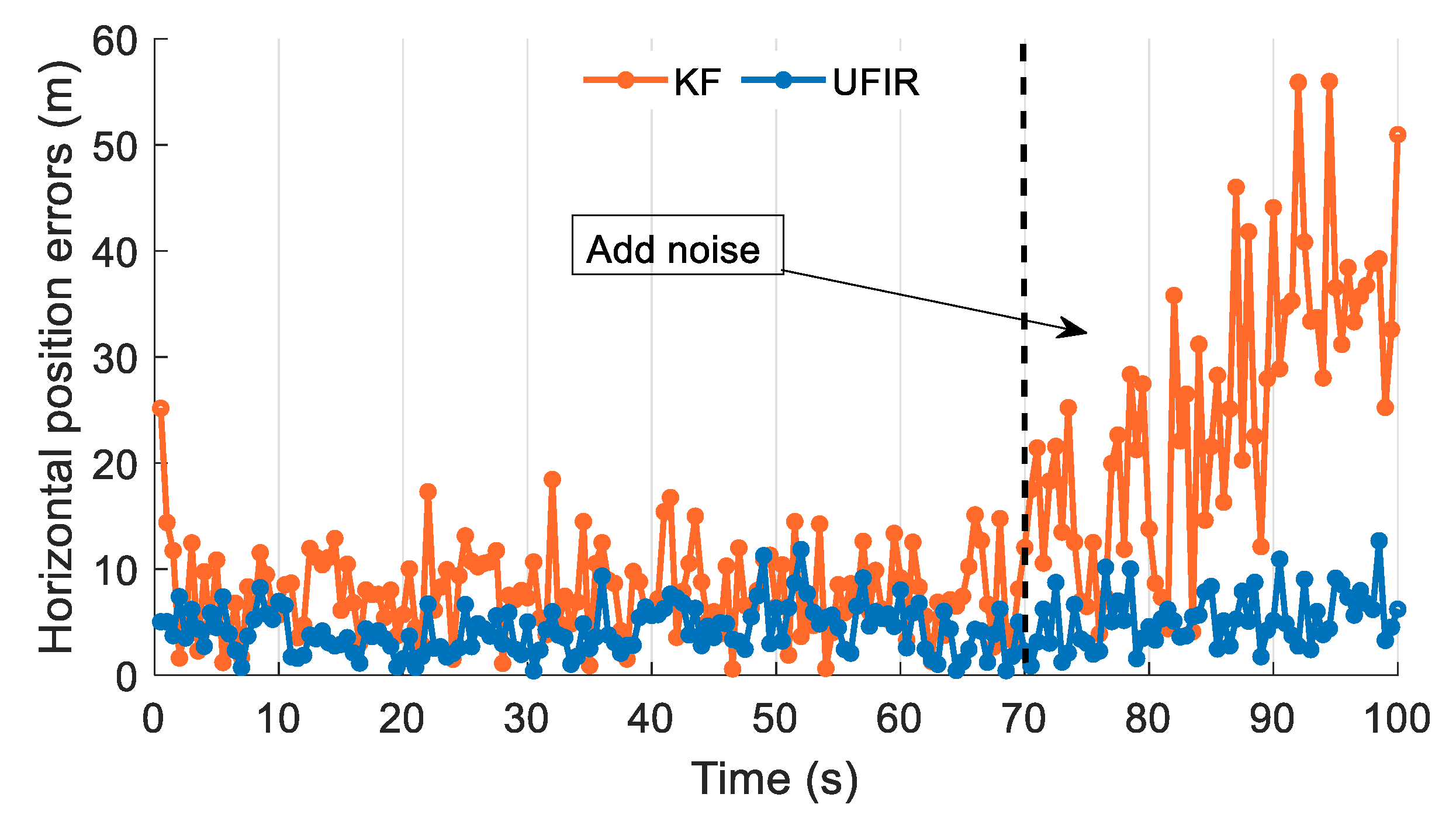
Because the UFIR operates only with the $N_{opt}$ adjacent points in a batch form, the accumulation of errors is ultimately suppressed.

(3)

Two field tests were conducted, and comparative analyses were performed with LS and KF methods. The results show that the UFIR solution can significantly improve GNSS positioning performance.

This paper is structured as follows. In Section 2, some formulas of GNSS positioning are given, and we also review the LS and KF approaches. In Section 3, we present the framework of the UFIR and its implementation in GNSS. In Section 4, two field tests are conducted, and the results of LS, KF, and UFIR are also presented, compared, and analyzed. Section 5 concludes this paper.

2. Problem Formulation

As mentioned earlier, the user PVT information is derived using the pseudorange and pseudorange rate observations. These observations are generated from two different tracking loops, which include the code tracking loop and the carrier tracking loop. This section sequentially introduces the parameterization model in operation and the estimation methods. Specifically, Section 2.1 presents GNSS formulas for position calculation; Section 2.2 gives the principle of the LS method; and Section 2.3 reviews the KF and its difference with LS.

2.1. GNSS Position Calculation

Figure 1 illustrates the geometric structure relating the satellite positions to the receiver’s location. Assuming there are i visible satellites, the pseudorange formulas are expressed as follows [6]:

$$\left\{\begin{array}{c}\sqrt{{(x_1-x_u)}^2+{(y_1-y_u)}^2+{(z_1-z_u)}^2}+c\cdot \delta t_u+I_1+T_1+{\epsilon }_1={\rho }_{ 1}\\ \sqrt{{(x_2-x_u)}^2+{(y_2-y_u)}^2+{(z_2-z_u)}^2}+c\cdot \delta t_u+I_2+T_2+{\epsilon }_2={\rho }_{ 2}\\ \hspace{1em}\hspace{1em}\hspace{1em}\hspace{1em}\hspace{1em}\hspace{1em}\hspace{1em}\hspace{1em}\hspace{1em}\hspace{1em}\hspace{1em}\hspace{1em}\hspace{1em}\hspace{1em}\hspace{1em}\hspace{1em}\hspace{1em}\hspace{1em}\hspace{1em}\hspace{1em} ⋮\\ \sqrt{{(x_i-x_u)}^2+{(y_i-y_u)}^2+{(z_i-z_u)}^2}+c\cdot \delta t_u+I_i+T_i+{\epsilon }_i={\rho }_{ i}\end{array}\right.$$

(1)

where $\mathit{x}={[x_u,y_u,z_u]}^T$ and ${\mathit{x}}_i={[x_i,y_i,z_i]}^T$ are the receiver’s position and the $i^{th}$ satellite position vectors in an earth-centered and earth-fixed (ECEF) frame, respectively; $\delta t_u$ is the receiver clock offset; ${\rho }_i$ denotes the pseudorange between the $i^{th}$ satellite and the GNSS receiver; $I_i$ and $T_i$ are ionospheric delay and tropospheric delay errors; ${\epsilon }_i$ represents other error factors, such as pseudorange noises and unmodeled random error; and $c$ denotes the speed of the light.

2.2. Least Square Method

In the above, each pseudorange measurement equation is a nonlinear function of the user position. After Taylor expansion and ignoring high-order terms, the relation between the offset $\mathsf{\Delta }\mathit{x}$ and pseudorange values $\mathsf{\Delta }\mathit{\rho }$ can be expressed as [6]:

$$\mathbf{H}\cdot \mathsf{\Delta }\mathit{x}=\mathsf{\Delta }\mathit{\rho }$$

(2)

where $\mathsf{\Delta }\mathit{x}={[\mathsf{\Delta }x \mathsf{\Delta }y \mathsf{\Delta }z c\cdot \delta t_u]}^T$ is the state increment of user receiver and $\mathsf{\Delta }\mathit{\rho }$ is the pseudorange increment; they represent the provision of the approximate solution around the linearization point and the linearization of the satellite–receiver geometric range, referring to $\mathsf{\Delta }\mathit{x}=\mathit{x}-{\mathit{x}}_0$ and $\mathsf{\Delta }\mathit{\rho }=\mathit{\rho }-{\mathit{\rho }}_0$. The receiver clock offset $\delta t_u$ is not affected by the linearization; $\mathbf{H}$ is the direction cosine matrix, given by:

$$\mathbf{H}={\left[\begin{array}{cccc}{e}_x^1& e_y^1& e_z^1& 1\\ e_x^2& e_y^2& e_z^2& 1\\ ⋮& ⋮& ⋮& ⋮\\ e_x^i& e_y^i& e_z^i& 1\end{array}\right]}_{i\times 4}$$

(3)

and the ${\mathit{e}}_i=[e_x^i e_y^i e_z^i]$ denotes the unit vector from the user location to the $i^{th}$ satellite, obtained by follows:

$$e_x^i=-\frac{x_i-x}{r_i}, e_y^i=-\frac{y_i-y}{r_i}, e_z^i=-\frac{z_i-z}{r_i}$$

(4)

where $r_i=\sqrt{{(x_i-x_u)}^2+{(y_i-y_u)}^2+{(z_i-z_u)}^2}$ is the approximate distance between the user and the $i^{th}$ satellite.

The $\mathsf{\Delta }\mathit{\rho }$ can be further expressed as:

$$\mathsf{\Delta }\mathit{\rho }={\left[\begin{array}{c}{\rho }_{ 1}-\sqrt{{(x_1-x_u)}^2+{(y_1-y_u)}^2+{(z_1-z_u)}^2}-c\cdot \delta t_u-I_1-T_1\\ {\rho }_{ 2}-\sqrt{{(x_2-x_u)}^2+{(y_2-y_u)}^2+{(z_2-z_u)}^2}-c\cdot \delta t_u-I_2-T_2\\ ⋮\\ {\rho }_{ i}-\sqrt{{(x_i-x_u)}^2+{(y_i-y_u)}^2+{(z_i-z_u)}^2}-c\cdot \delta t_u-I_i-T_i\end{array}\right]}_{i\times 1}$$

(5)

According to Equation (2), the state increment of the user receiver can be written as:

$$\mathsf{\Delta }\mathit{x}={({\mathbf{H}}^{\mathrm{T}}\mathbf{H})}^{-1}{\mathbf{H}}^{\mathrm{T}}\cdot \mathsf{\Delta }\mathit{\rho }$$

(6)

Accordingly, one can express the update of the position estimation and the receiver clock bias by adding the position increment $\mathsf{\Delta }\mathit{x}$ to the current state, as follows:

$${\mathit{x}}_{k+1}={\mathit{x}}_k+\mathsf{\Delta }\mathit{x}$$

(7)

As we can see from the above, the LS method considers that each measurement is independent of each other, and it provides a single estimate of the position that fits the observed measurements. This indicates that the relationship between these measurements has not been investigated.

2.3. Kalman Filter

The KF is typically a state-space approach utilized for estimating the state of a dynamic system while considering noisy observations. It involves the use of both the state vector and the measurement vector in the estimation process. In general, the adjacent state vector $\mathsf{\Delta }\mathbf{x}$ can be modeled as [27]:

$$\mathsf{\Delta }\mathbf{x}={[\mathsf{\Delta }{x}_k \mathsf{\Delta }{y}_k \mathsf{\Delta }{z}_k \mathsf{\Delta }{v}_{x,k} \mathsf{\Delta }{v}_{y,k} \mathsf{\Delta }{v}_{z,k} c\mathsf{\Delta }{t}_k c\mathsf{\Delta }{\dot{t}}_k]}^T$$

(8)

where $\mathsf{\Delta }{v}_x,\mathsf{\Delta }{v}_y,\mathsf{\Delta }{v}_z$, and $c\cdot \mathsf{\Delta }\dot{t}$ present the velocity deviation of the user and clock drift.

Thus, the state propagation equation at epoch k can be given by:

$$\mathsf{\Delta }{\mathbf{x}}_{k|k-1}={\mathbf{\Phi }}_{k-1}\cdot \mathsf{\Delta }{\mathbf{x}}_k+{\mathbf{w}}_{k-1}$$

(9)

$${\mathbf{\Phi }}_{k-1}={\left[\begin{array}{ccc}{\mathbf{I}}_{3\times 3}& \tau \cdot {\mathbf{I}}_{3\times 3}& {\mathbf{0}}_{3\times 2}\\ {\mathbf{0}}_{3\times 3}& {\mathbf{I}}_{3\times 3}& {\mathbf{0}}_{3\times 2}\\ {\mathbf{0}}_{2\times 3}& {\mathbf{0}}_{2\times 3}& \mathbf{K}\end{array}\right]}_{8\times 8}, \mathbf{K}=\left[\begin{array}{cc}1& \tau \\ 0& 1\end{array}\right]$$

(10)

in which $\mathbf{\Phi }$ denotes the system transition matrix; $\mathbf{w}$ is the process noise term; $\mathbf{I}$ denotes an identity matrix; and $\tau$ is the update interval of the KF.

The process noise covariance matrix $\mathit{Q}$ that related to $\mathbf{w}$ is determined based on the rule of thumb, which takes into consideration the user dynamics and oscillator used. The calculation is performed as follows [27]:

$$\mathit{Q}={\left[\begin{array}{cc}{\mathit{Q}}_{dyn}& {\mathbf{0}}_{6\times 2}\\ {\mathbf{0}}_{2\times 6}& {\mathit{Q}}_{clk}\end{array}\right]}_{8\times 8}$$

(11)

$${\mathit{Q}}_{dyn}={\left[\begin{array}{cc}\mathsf{\Delta }{t}^3/3\cdot {\mathbf{I}}_{3\times 3}& \mathsf{\Delta }{t}^2/2\cdot {\mathbf{I}}_{3\times 3}\\ \mathsf{\Delta }{t}^2/2\cdot {\mathbf{I}}_{3\times 3}& \mathsf{\Delta }t\cdot {\mathbf{I}}_{3\times 3}\end{array}\right]}_{6\times 6}\cdot S_v$$

(12)

$${\mathit{Q}}_{clk}=\left[\begin{array}{cc}{S}_f\cdot \mathsf{\Delta }t+S_f\cdot \mathsf{\Delta }{t}^3/3& S_g\cdot \mathsf{\Delta }{t}^2/2\\ S_g\cdot \mathsf{\Delta }{t}^2/2& S_g\cdot \mathsf{\Delta }t\end{array}\right]$$

(13)

where $S_v$ represents noise power spectral density (PSD) of the receiver velocity, set by the level of user dynamics; and $S_f$ and $S_g$ are the PSD of receiver clock phase and frequency, respectively, calculated as follows:

$$S_f=c^2\cdot h_0/2$$

(14)

$$S_g=c^2\cdot 2{\pi }^2\cdot h_{-2}$$

(15)

where $h_0$ and $h_{-2}$ represent the clock model coefficients associated with the white frequency modulation noise and random walk frequency modulation noise, respectively, associated with the utilized oscillator.

The covariance matrix ${\mathbf{P}}_k$ of the priori sate estimation can be expressed as:

$${\mathbf{P}}_k=\mathbf{\Phi }{\mathbf{P}}_{k-1}{\mathbf{\Phi }}^T+{\mathbf{Q}}_{k-1}$$

(16)

The linearized GNSS measurement equation is given as follows:

$${\mathbf{y}}_k=\left[\begin{array}{c}\mathsf{\Delta }{\mathit{\rho }}_k\\ \mathsf{\Delta }{\dot{\mathit{\rho }}}_k\end{array}\right]={\mathbf{H}}_k\cdot {\mathbf{x}}_{k-1}+{\mathbf{v}}_k$$

(17)

where $\mathbf{H}$ is the measurement matrix, given by:

$${\mathbf{H}}_k={\left[\begin{array}{cccccccc}{e}_{x,k}^1& e_{y,k}^1& e_{z,k}^1& 0& 0& 0& 1& 0\\ e_{x,k}^2& e_{y,k}^2& e_{z,k}^2& 0& 0& 0& 1& 0\\ ⋮& ⋮& ⋮& ⋮& ⋮& ⋮& ⋮& ⋮\\ e_{x,k}^N& e_{y,k}^N& e_{z,k}^N& 0& 0& 0& 1& 0\\ 0& 0& 0& e_{x,k}^1& e_{y,k}^1& e_{z,k}^1& 0& 1\\ 0& 0& 0& e_{x,k}^2& e_{y,k}^2& e_{z,k}^2& 0& 1\\ ⋮& ⋮& ⋮& ⋮& ⋮& ⋮& ⋮& ⋮\\ 0& 0& 0& e_{x,k}^N& e_{y,k}^N& e_{z,k}^N& 0& 1\end{array}\right]}_{2N\times 8}$$

(18)

in which $\mathsf{\Delta }\mathit{\rho }$ and $\mathsf{\Delta }\dot{\mathit{\rho }}$ are the pseudorange increment and pseudorange rate increment, respectively; ${\mathbf{v}}_k$ is the measurement noise vector.

Unlike the process noise, the measurement noise depends on the particular phase discriminator implementation, and its covariance matrix is calculated by:

$${\mathbf{R}}_k=\mathrm{d}\mathrm{i}\mathrm{a}\mathrm{g}(\sigma ({\mathbf{\gamma }}_k))$$

(19)

where $\sigma (x)$ is the variance of x, diag(·) represents a diagonal matrix, and ${\mathbf{\gamma }}_k={\mathbf{y}}_k-{\mathbf{H}}_k{\mathbf{x}}_k$ is referred to as the measurement residual or innovation sequence.

Therefore, it suffices to update the posteriori state estimation based on the innovation ${\mathbf{\gamma }}_k$, using [28]:

$${\mathbf{x}}_k={\mathbf{x}}_{k|k-1}+{\mathbf{K}}_k{\mathbf{\gamma }}_k$$

(20)

in which ${\mathbf{K}}_k$ denotes the state feedback gain matrix, given by:

$${\mathbf{K}}_k={\mathbf{P}}_k{\mathbf{H}}_k^T{({\mathbf{R}}_k+{\mathbf{H}}_k{\mathbf{P}}_k{\mathbf{H}}_k^T)}^{-1}$$

(21)

The updated covariance matrix is defined by:

$${\mathbf{P}}_k^{-}=(\mathbf{I}-{\mathbf{K}}_k{\mathbf{H}}_k){\mathbf{P}}_k$$

(22)

Incorporating the updated state estimation, ${\mathbf{x}}_k$, the final state of the user receiver is obtained by:

$${\mathbf{x}}_k^{usr}=\mathbf{\Phi }{\mathbf{x}}_{k|k-1}+{\mathbf{x}}_k$$

(23)

Unlike the LS, the KF considers that each measurement is time-correlated because state transformation constraints are included. In addition, KF makes an error analysis of the current estimation and aims to minimize the variance of the state error. Compared to the results obtained from the LS method, utilizing the KF approach yields smoother and more authentic results. Nonetheless, because of the sensitivity to noise uncertainty and because the historical information has not been explored, the improvement is limited. A framework that possesses historical information constraints and that is noise independent is anticipated to produce superior estimate results compared to the LS and KF.

3. Optimization Framework

In this section, the UFIR optimization framework is proposed to obtain superior position estimates. To this end, the extended state-space model is first constructed. Then, the posterior estimation, error covariance, and gain of UFIR are described in detail. Finally, the way to find the optimal horizon length is given.

3.1. Extended Model

For UFIR, the extended state vector ${\mathbf{X}}_{n,m}$ and observation vector ${\mathbf{Y}}_{n,m}$ are represented in a horizon length of N epochs, within the interval $[m=n-N+1,n]$. Accordingly, Equations (9) and (17) can first be rewritten using the time-forward solution by [29]:

$${\mathbf{X}}_{n,m}={\mathbf{\Phi }}_{n,m}{\mathbf{x}}_{m-1}+{\mathbf{G}}_{n,m}{\mathbf{W}}_{n,m}$$

(24)

$${\mathbf{Y}}_{n,m}={\mathbf{H}}_{n,m}{\mathbf{x}}_{m-1}+{\mathbf{L}}_{n,m}{\mathbf{W}}_{n,m}+{\mathbf{V}}_{n,m}$$

(25)

where ${\mathbf{X}}_{n,m}={[{\mathbf{x}}_n^T,{\mathbf{x}}_{n-1}^T,\cdots ,{\mathbf{x}}_m^T]}^T$, ${\mathbf{Y}}_{n,m}={[{\mathbf{y}}_n^T,{\mathbf{y}}_{n-1}^T,\cdots ,{\mathbf{y}}_m^T]}^T$, ${\mathbf{W}}_{n,m}={[{\mathbf{w}}_n^T,{\mathbf{w}}_{n-1}^T,\cdots ,{\mathbf{w}}_m^T]}^T$ and ${\mathbf{V}}_{n,m}={[{\mathbf{v}}_n^T,{\mathbf{v}}_{n-1}^T,\cdots ,{\mathbf{v}}_m^T]}^T$ are the extended vectors.

The extended matrices ${\mathbf{\Phi }}_{n,m}$, ${\mathbf{G}}_{n,m}$, ${\mathbf{H}}_{n,m}$ and ${\mathbf{L}}_{n,m}$ are provided by, respectively,

$${\mathbf{\Phi }}_{n,m}={[{({\mathcal{F}}_n^m)}^T,{({\mathcal{F}}_{n-1}^m)}^T,\cdots ,{\mathbf{\Phi }}_m^T]}^T$$

(26)

$${\mathbf{G}}_{n,m}=\left[\begin{array}{ccccc}{\mathbf{G}}_n& {\mathbf{\Phi }}_n{\mathbf{G}}_{n-1}& \cdots & {\mathcal{F}}_n^{m+2}{\mathbf{G}}_{m+1}& {\mathcal{F}}_n^{m+1}{\mathbf{G}}_m\\ \mathbf{0}& {\mathbf{G}}_{n-1}& \cdots & {\mathcal{F}}_{n-1}^{m+2}{\mathbf{G}}_{m+1}& {\mathcal{F}}_{n-1}^{m+1}{\mathbf{G}}_m\\ ⋮& ⋮& \ddots & ⋮& ⋮\\ \mathbf{0}& \mathbf{0}& \cdots & {\mathbf{G}}_{m+1}& {\mathbf{\Phi }}_{m+1}{\mathbf{G}}_m\\ \mathbf{0}& \mathbf{0}& \cdots & \mathbf{0}& {\mathbf{G}}_m\end{array}\right]$$

(27)

${\mathbf{H}}_{n,m}={\overline{\mathbf{H}}}_{n,m}{\mathbf{\Phi }}_{n,m}$, ${\mathbf{L}}_{n,m}={\overline{\mathbf{H}}}_{n,m}{\mathbf{G}}_{n,m}$ with ${\overline{\mathbf{H}}}_{n,m}=\mathrm{d}\mathrm{i}\mathrm{a}\mathrm{g}({\mathbf{H}}_n,{\mathbf{H}}_{n-1},\cdots ,{\mathbf{H}}_m)$, and ${\mathcal{F}}_n^m={\mathbf{\Phi }}_n{\mathbf{\Phi }}_{n-1}\cdots {\mathbf{\Phi }}_m$. Generally, matrix $\mathbf{G}$ is set as the identity matrix $\mathbf{I}$, and $\mathbf{\Phi }$ is time invariant. The noise vectors ${\mathbf{w}}_n$ and ${\mathbf{v}}_n$ are both white, and the corresponding variance matrices related to the extended model are ${\mathbf{Q}}_{n,m}=\mathrm{d}\mathrm{i}\mathrm{a}\mathrm{g}({\mathbf{Q}}_n,{\mathbf{Q}}_{n-1},\cdots ,{\mathbf{Q}}_m)$ and ${\mathbf{R}}_{n,m}=\mathrm{d}\mathrm{i}\mathrm{a}\mathrm{g}({\mathbf{R}}_n,{\mathbf{R}}_{n-1},\cdots ,{\mathbf{R}}_m)$. The details of the expanded state-space model can be further explored in reference [23].

3.2. UFIR Estimator

From the extended state dynamic Equation (24), state $\mathbf{x}$ with respect to ${\mathbf{x}}_{m-1}$ can be represented as:

$${\mathbf{x}}_n={\mathcal{F}}_n^m{\mathbf{x}}_{m-1}+{\mathcal{W}}_{n,m}$$

(28)

where ${\mathcal{W}}_{n,m}={\overline{\mathbf{G}}}_{n,m}{\mathbf{W}}_{n,m}$ and ${\overline{\mathbf{G}}}_{n,m}\triangleq [{\mathbf{G}}_n,{\mathbf{\Phi }}_n{\mathbf{G}}_{n-1},\cdots ,{\mathcal{F}}_n^{m+2}{\mathbf{G}}_{m+1},{\mathcal{F}}_n^{m+1}{\mathbf{G}}_{n-1}]$ are the first-row vectors of ${\mathbf{G}}_{n,m}$. Combining Equations (25) and (28), the measurement equation becomes:

$${\mathbf{y}}_n={\tilde{\mathbf{H}}}_{n,m}{\mathbf{x}}_n+{\mathcal{L}}_{n,m}$$

(29)

where ${\tilde{\mathbf{H}}}_{n,m}={\mathbf{H}}_{n,m}{({\mathcal{F}}_n^m)}^{-1}$, and ${\mathcal{L}}_{n,m}=({\mathbf{L}}_{n,m}-{\tilde{\mathbf{H}}}_{n,m}{\overline{\mathbf{G}}}_{n,m}){\mathbf{W}}_{n,m}+{\mathbf{V}}_{n,m}$.

Given the extended matrices, the batch UFIR estimate ${\hat{\mathbf{x}}}_n$ at n epoch using the discrete convolution is [30]:

$${\hat{\mathbf{x}}}_n={\mathbf{\Phi }}^N{({\mathbf{H}}_{n,m}^T{\mathbf{H}}_{n,m})}^{-1}{\mathbf{H}}_{n,m}^T{\mathbf{Y}}_{n,m}$$

(30)

Equation (30) can be further computed in an iterative form, as:

$${\widehat{\mathbf{x}}}_j^{-}=\mathbf{\Phi }{\widehat{\mathbf{x}}}_j^{-}$$

(31)

$${\mathbf{G}}_j={[{\mathbf{H}}^T\mathbf{H}+{(\mathbf{\Phi }{\mathbf{G}}_{j-1}{\mathbf{\Phi }}^T)}^{-1}]}^{-1}$$

(32)

$${\hat{\mathbf{x}}}_j={\hat{\mathbf{x}}}_j^{-}+{\mathbf{G}}_j{\mathbf{H}}^T({\mathbf{y}}_j-\mathbf{H}{\hat{\mathbf{x}}}_j^{-})$$

(33)

where $j\in [m+a, n]$ and ${\mathbf{G}}_j$ and ${\widehat{\mathbf{x}}}_j$ are initialized in short batch form as:

$${\mathbf{G}}_{j=m+a-1}={\mathbf{\Phi }}^a{({\mathbf{H}}_a^T{\mathbf{H}}_a)}^{-1}{\mathbf{\Phi }}^{a^T}$$

(34)

$${\widehat{\mathbf{x}}}_{j=m+a-1}={\mathbf{\Phi }}^a{({\mathbf{H}}_a^T{\mathbf{H}}_a)}^{-1}{\mathbf{H}}_a^T{\mathbf{Y}}_{m+a-1}$$

(35)

where a represents the dimension of the state ${\mathbf{x}}_n$.

Furthermore, the error covariance ${\mathbf{P}}_j$ can be calculated using the following method:

$${\mathbf{P}}_j=(\mathbf{I}-{\mathbf{\Xi }}_j\mathbf{H})(\mathbf{\Phi }{\mathbf{P}}_{j-1}{\mathbf{\Phi }}^T+{\mathbf{Q}}_j){(\mathbf{I}-{\mathbf{\Xi }}_j\mathbf{H})}^T+{\Xi }_j{\mathbf{R}}_j{\mathbf{\Xi }}_j^T$$

(36)

in which ${\mathbf{\Xi }}_j={\mathbf{G}}_j{\mathbf{H}}^T$ denotes the UFIR filter gain that is used to correct the bias. The initial covariance matrix is given by:

$${\mathbf{P}}_{m+a-1}=({\mathbf{K}}_a{\mathbf{H}}_a-{\overline{\mathbf{G}}}_a){\mathbf{Q}}_{m+a-1}{(\cdots )}^T+{\mathbf{K}}_a{\mathbf{R}}_{m+a-1}{\mathbf{K}}_a^T$$

(37)

with gain

$${\mathbf{K}}_a={\mathbf{\Phi }}^a{({\mathbf{H}}_a^T{\mathbf{H}}_a)}^{-1}{\mathbf{H}}_a^T$$

(38)

It is important to note that matrix $\mathbf{\Xi }$, which is used to correct the estimation bias in UFIR, is determined by $\mathbf{H}$ and $\mathbf{\Phi }$, which are already known. However, the gain of KF depends not only on the process noise $\mathbf{Q}$ but also on the measurement noise $\mathbf{R}$, making it challenging to set them perfectly. This distinctive feature makes UFIR more robust than KF against the errors of noise statistics. It is also noteworthy that UFIR requires the horizon length $N$ to be optimal, which will be given in the next section.

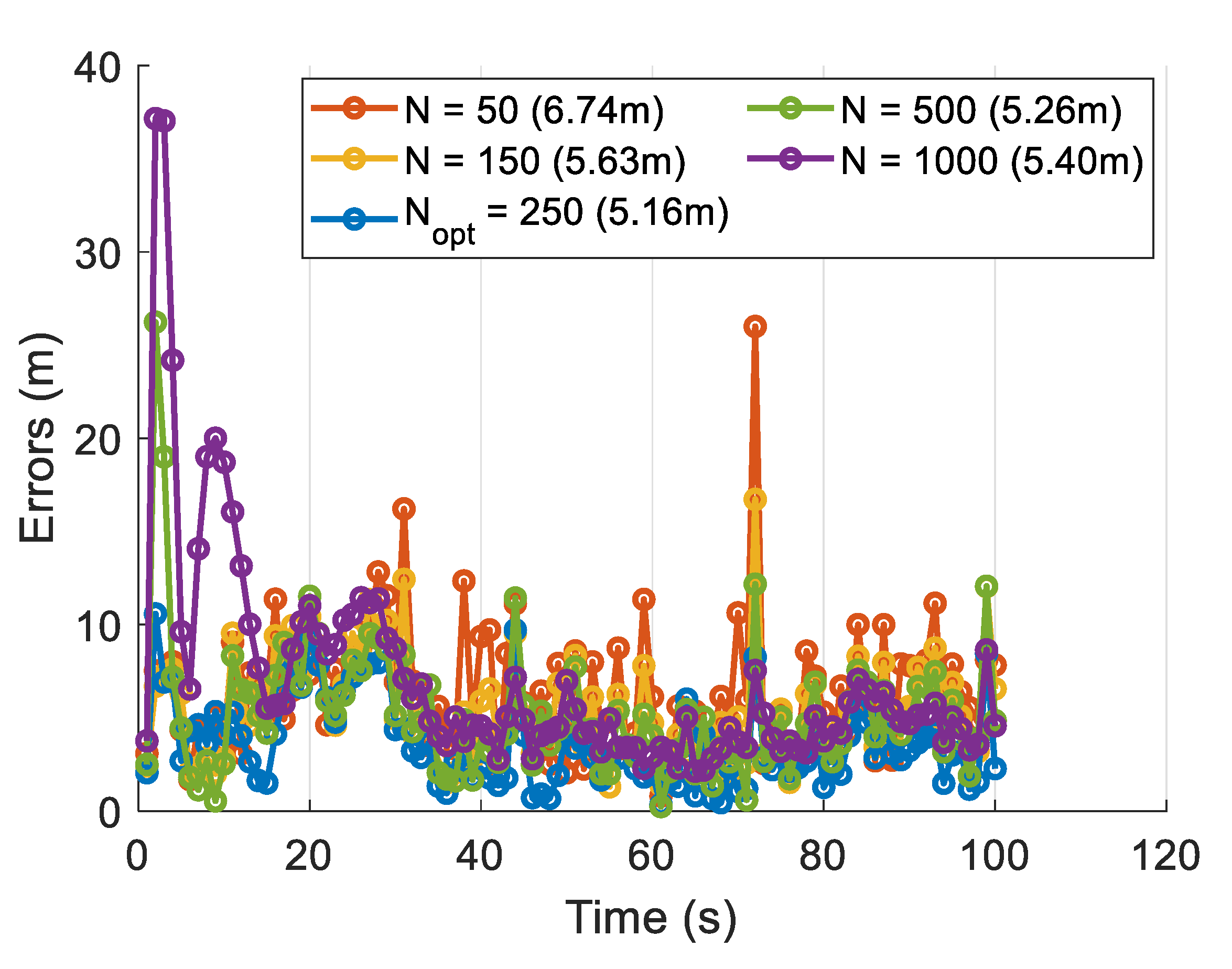
3.3. Turning of UFIR

For the UFIR strategy, the objective of $N_{opt}$ is to minimize the MSE. The memory length $N_{opt}$ is the critical tuning parameter that ensures UFIR is optimal. When $N<N_{opt}$, the UFIR fits with the model well, but the noise reduction is insufficient. Alternatively, the bias errors become dominant. This is because the UFIR no longer fits with the model, although it better suppresses the noise.

Generally, if the ground truth is available in the operation, then $N_{opt}$ can be provided by [31]:

$$N_{opt}=\underset{N}{\mathrm{a}\mathrm{r}\mathrm{g}\mathrm{m}\mathrm{i}\mathrm{n}}\left\{\mathrm{t}\mathrm{r}{\mathbf{P}}_k(N)\right\}$$

(39)

where $\mathrm{t}\mathrm{r}(\cdot )$ denotes the trace operator and $\mathrm{a}\mathrm{r}\mathrm{g}\mathrm{m}\mathrm{i}\mathrm{n}\left\{\cdot \right\}$ is the minimization operator.

Otherwise, an alternative approach is given as follows:

$$N_{opt}\cong \underset{N}{\mathrm{a}\mathrm{r}\mathrm{g}\mathrm{m}\mathrm{i}\mathrm{n}}\left\{\frac{\partial }{\partial k}\mathrm{t}\mathrm{r}{\mathcal{V}}_k(N)\right\}$$

(40)

where ${\mathcal{V}}_k=\mathcal{E}\left\{({\mathbf{y}}_k-{\mathbf{H}}_k{\hat{\mathbf{x}}}_k^{-}){({\mathbf{y}}_k-{\mathbf{H}}_k{\hat{\mathbf{x}}}_k^{-})}^T\right\}$ is the mean-square value.

4. Experiments and Results

In this section, we conducted land-vehicle experiments and collected data from real scenarios to assess the efficiency of the proposed approach. To be specific, two separate experiments were performed in different areas: one in an urban environment and the other in a suburban environment, utilizing authentic GNSS signal reception. These scenarios were selected based on frequent occurrence challenges in the field to the majority of GNSS applications. By examining these common and representative situations, we aim to ensure that our findings are not limited to niche cases but have broader applicability and relevance across a range of scenarios. Experimental results derived from these scenarios can be generalized to many similar situations in GNSS solutions. Furthermore, the existing LS and KF positioning methods are also employed as benchmarks for a fair comparison and analysis.

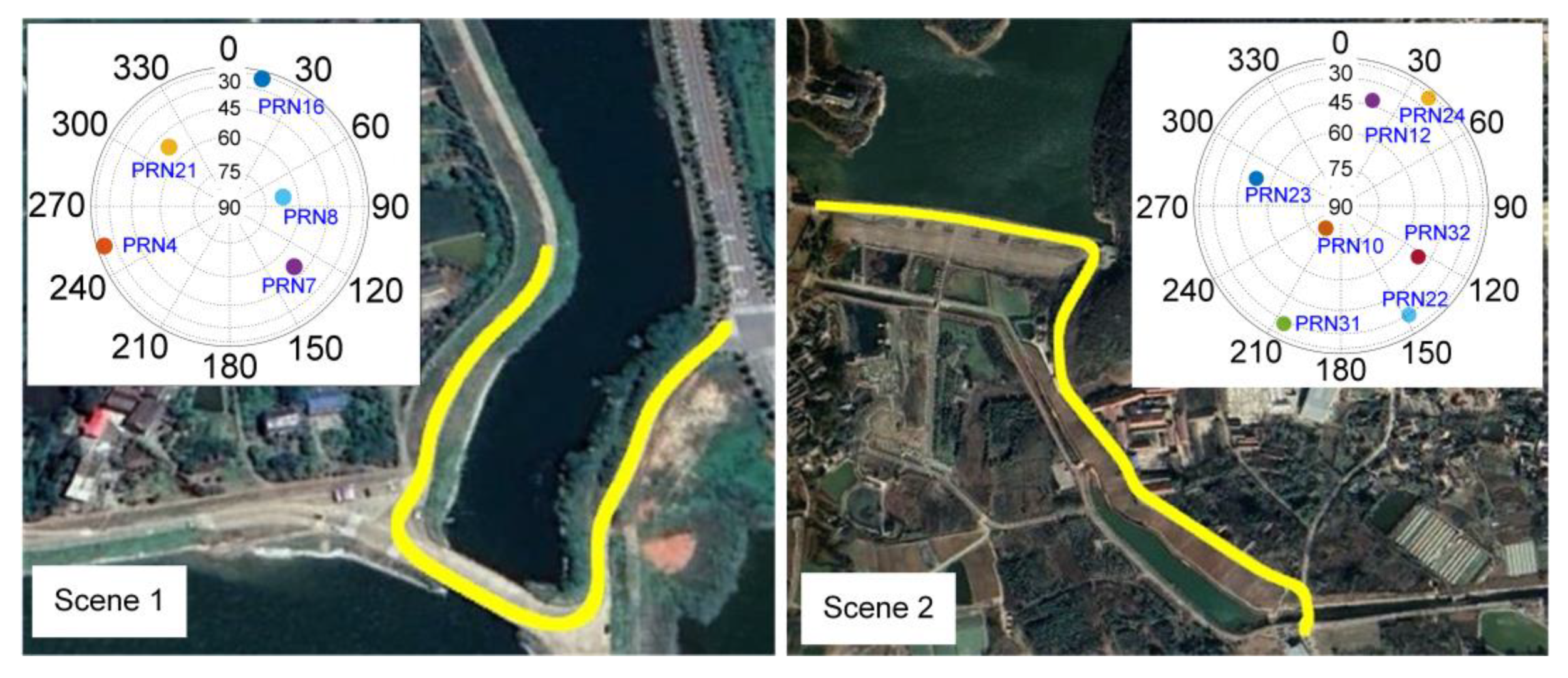
4.1. Data Description

To verify the proposed method, we utilized datasets collected from two different scenarios. Figure 2 illustrates the experimental setup, in which two GNSS antennas were mounted on the top of the car. A commercial U-blox NEO-M8T GNSS receiver, sourced from u-blox, Thalwil, Switzerland, was employed for providing a ground truth of positioning, at a frequency of 2 Hz. The raw signal was first collected by a GNSS IF front-end sampler and then stored on a laptop. Finally, the raw IF data were processed by a GNSS software-defined receiver (SDR), version 1.0, which is developed based on MATLAB. The SDR processing was conducted using a laptop equipped with an Intel Core i5-12400H processor, running at 4.4 GHz and 16 GB of RAM. The processor is a product of Intel Corporation, headquartered in Santa Clara, CA, USA. Detailed configurations of the equipment are listed in

Table 1. Parameter settings of the experimental equipment.

Equipment	Parameter	Value	Unit
Antenna	Polarization	Right-hand circularly polarized (RHCP)	-
	Low noise amplifier (LNA) gain	32 ± 3.0	dB
	Elevation coverage	360°	-
	Noise figure	<2.0	dB
Front-end	GNSS signal	GPS L1	-
	Sampling rate	16.368	MHz
	IF	4.092	MHz
	IF bandwidth	2.5	MHz
	Quantization	IQ-2	bit
U-blox NEO-M8T	Channel	72	-
	Horizontal position accuracy	2.0 (Typical) 2.5 (SBAS)	m
	Position update rate	10 (Max)	Hz
	Channel	72	-

.

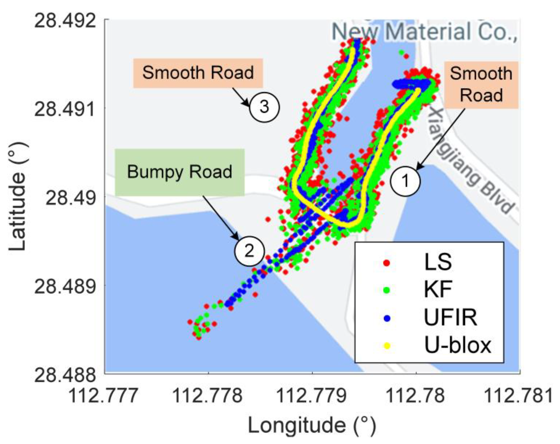
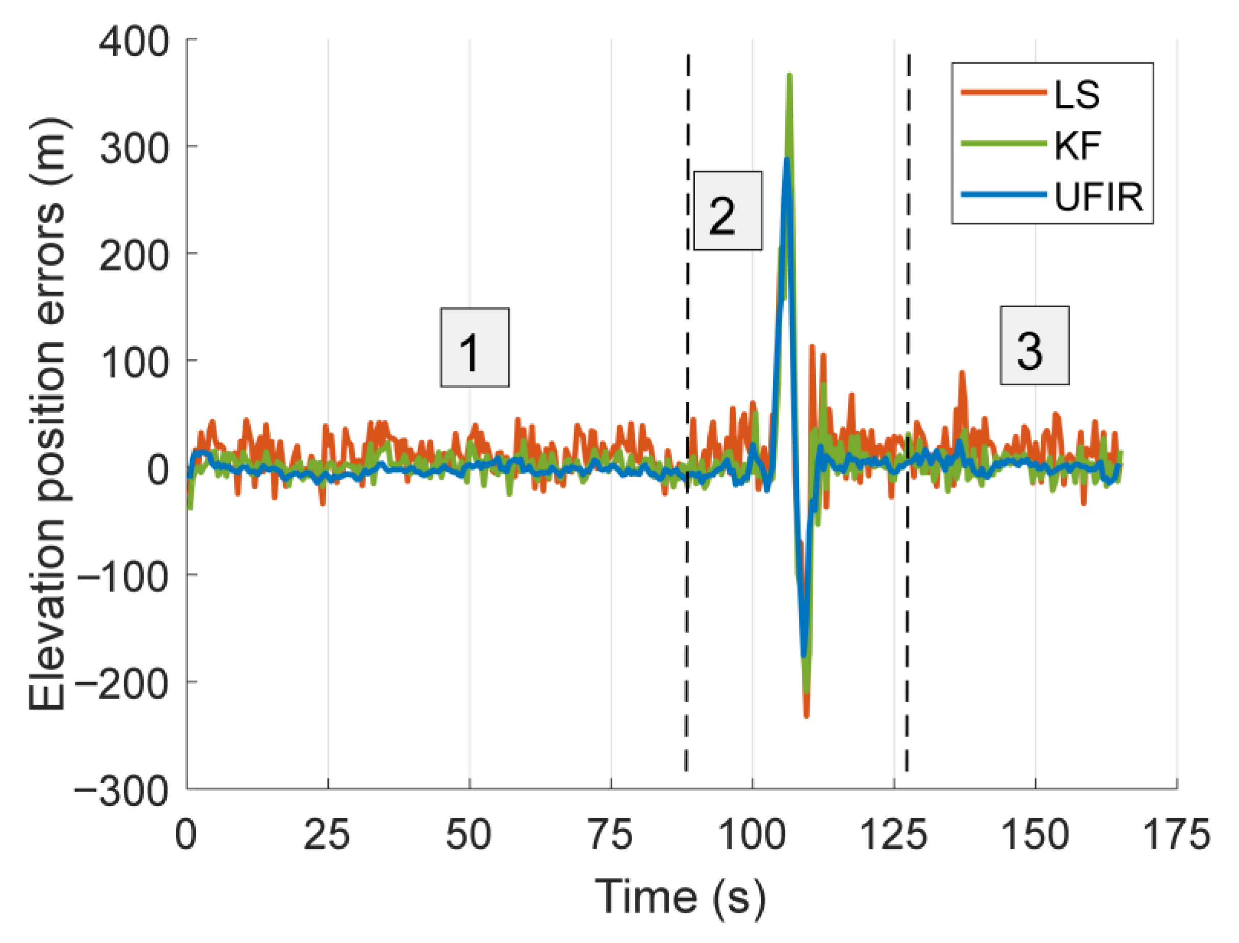
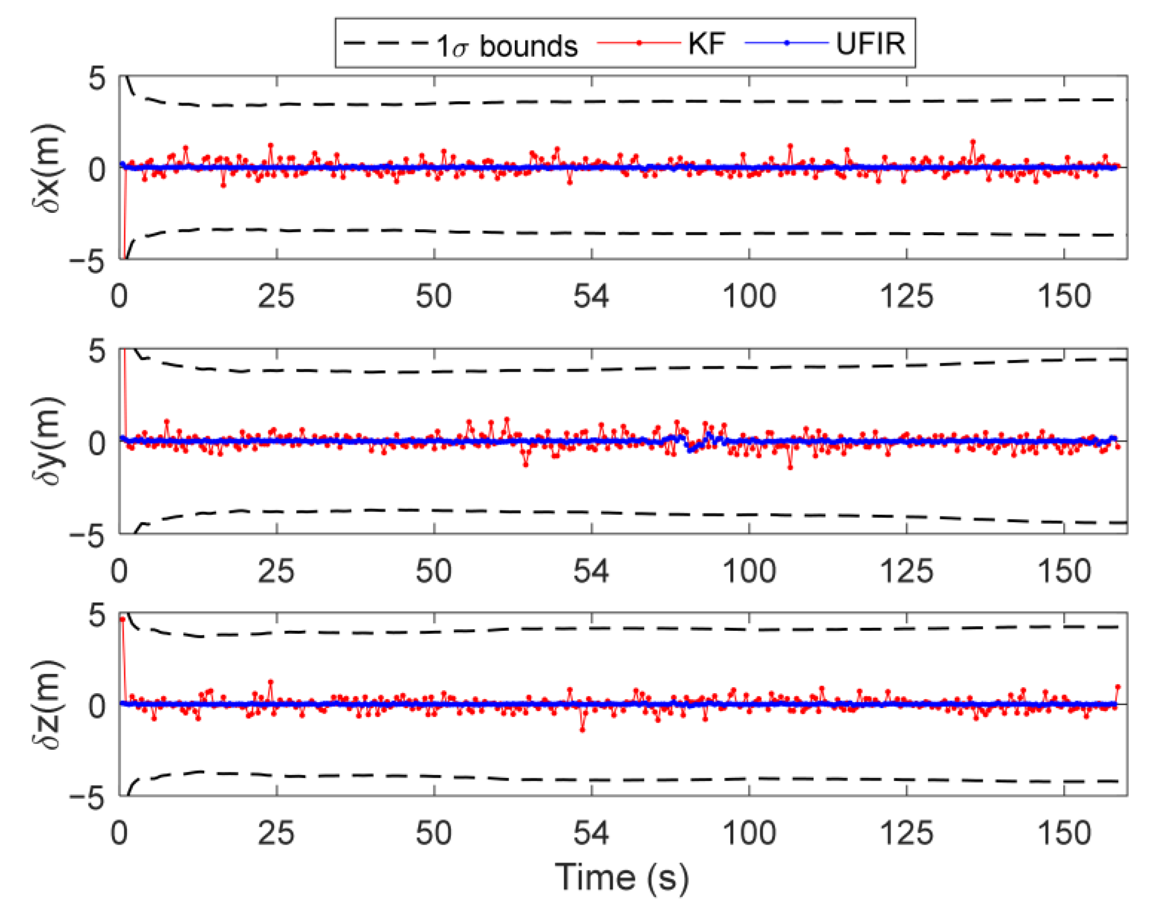
4.2. Positioning Performance Evaluation

Figure 3 shows two test trajectories and satellite views plotted on Google Earth. The test scenarios were classified into two types: bumpy road sections (Scene 1) and smooth road sections (Scene 2). During Scene 1, only five satellites were visible due to blocked GNSS signals, and the experiment lasted for 165 s. For the second test, an open area with no obstructions was chosen, and the experiment lasted for 245 s with a total of seven satellites available.

In KF, the error state covariance matrix ${\mathbf{P}}_0^{-}$ (unit: squared meter) and $\mathsf{\delta }{\mathit{x}}_0$ (unit: meter) are initialized as follows:

$${\mathbf{P}}_0^{-}=\mathrm{1}\mathrm{e}5\times \mathrm{d}\mathrm{i}\mathrm{a}\mathrm{g} [0.1,0.1,0.1,0.1,0.1,0.1,1,1]$$

(41)

$$\mathsf{\delta }{\mathit{x}}_0=\mathrm{d}\mathrm{i}\mathrm{a}\mathrm{g} [0,0,0,0,0,0,0,0]$$

(42)

The process and measurement noise covariance matrices, expressed in squared meters, are initialized as follows [27]:

$$\mathbf{Q}=\mathrm{d}\mathrm{i}\mathrm{a}\mathrm{g} [0.2,0.2,0.2,0.1,0.1,0.1,0.1,0.01]$$

(43)

$$\mathbf{R}=\left[\begin{array}{cc}0.3\times {\mathbf{I}}_m& \mathbf{0}\\ \mathbf{0}& 0.1\times {\mathbf{I}}_m\end{array}\right]$$

(44)

where $\mathrm{d}\mathrm{i}\mathrm{a}\mathrm{g}[\cdot ]$ represents a diagonal matrix; $\mathbf{I}$ is an identity matrix of dimension m; and m is the number of the tracking channel. The observation noise covariance matrix is then adaptively computed by Equation (19). The horizon lengths of these two tests are calculated using Equation (39)—specifically, $N_{opt}=150$ in the first test and $N_{opt}=250$ in the second test.

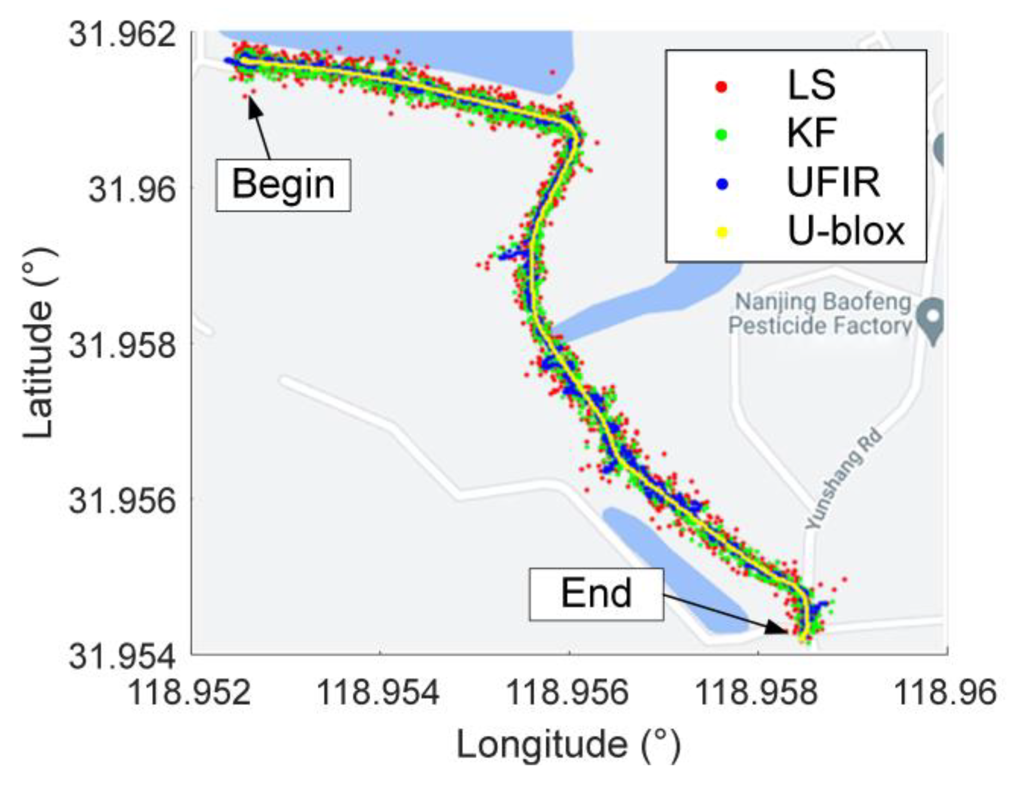
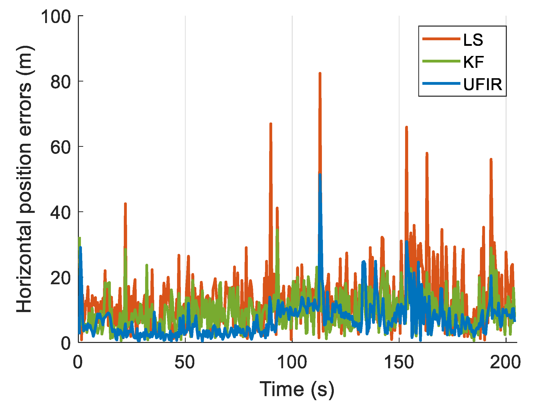
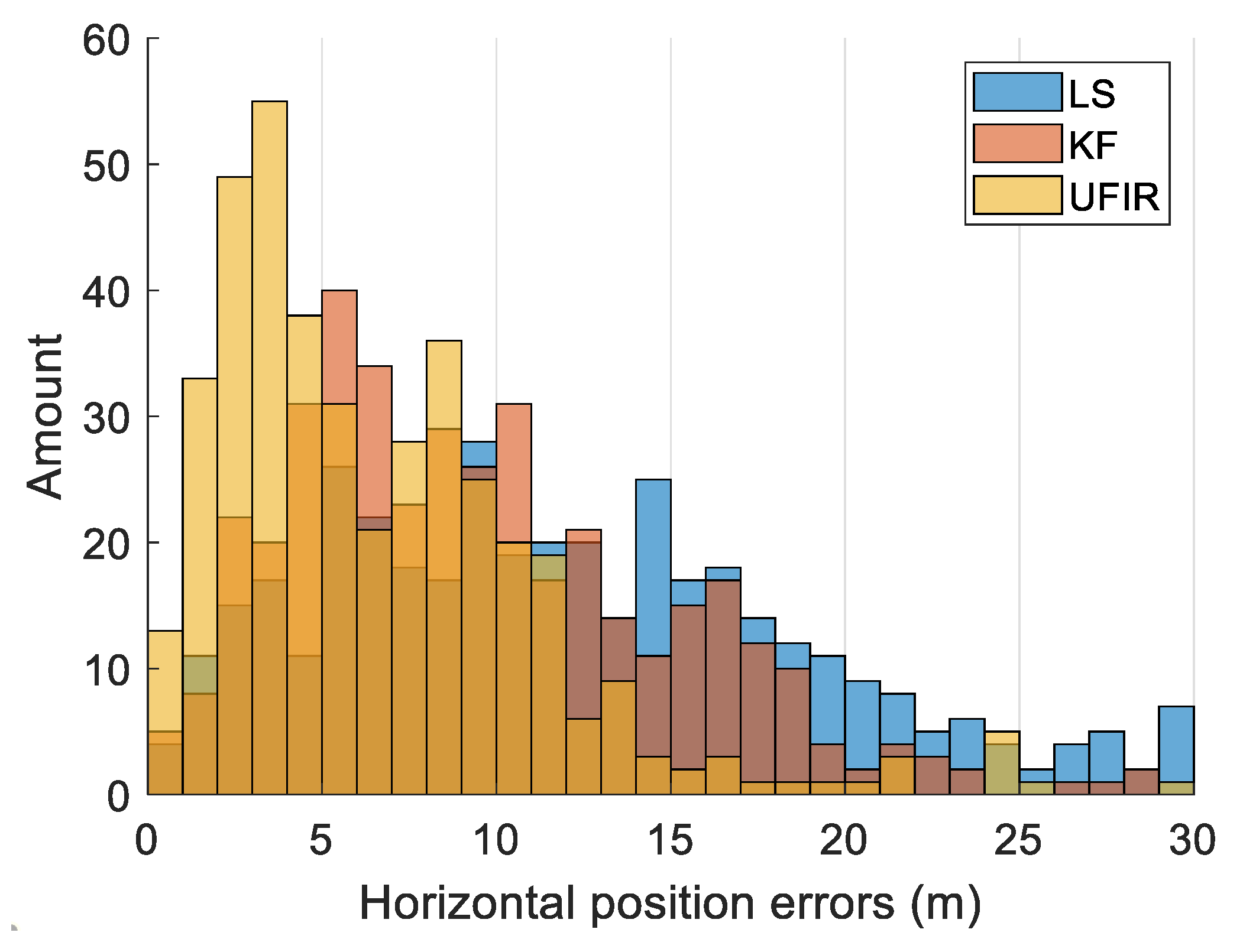
4.2.1. Test I: Urban Area, Bumpy Road

The positioning results in the horizontal direction for the LS, KF, and UFIR correction are illustrated in Figure 4. The horizon positioning error and elevation positioning error of these three methods are presented in Figure 5 and Figure 6, respectively. The entire driving route is divided into three periods. The car travels relatively smoothly in the first and third periods. As we can see, in the first- and third-time intervals, the errors obtained by the LS algorithm were the most significant, with horizontal positioning errors of approximately 11 m and vertical positioning errors of 24 m. The positioning results of the KF algorithm outperformed those of the LS, reducing the horizontal positioning error to around 8 m and the vertical error to 20 m. When employing the UFIR method, the horizontal and vertical positioning errors were further improved to 5.79 m and 15 m, respectively. The results indicate that the UFIR method is markedly superior to the other two algorithms. However, in the second period, the car encounters a bumpy road. We consider this situation as process interference. The reason is that the tilt of the antenna causes a decrease in GNSS signal gain. In this case, as a result, the positioning errors of all three methods have diverged. Specifically, the maximum horizontal positioning error for LS reached 165 m, while for KF it was 147 m, and for UFIR, it was reduced to 124 m. It is also observed that the LS algorithm yields the largest positioning error. Although the KF algorithm shows some improvement in positioning accuracy, the enhancement is limited, while the positioning results of the UFIR-based GNSS solution method are relatively smooth. The comparative results illustrate that, in terms of position accuracy, the relationship between these filters is LS < KF < UFIR.

Accordingly, the quantitated horizontal position results of LS, KF, and UFIR have been listed in

Table 2. Statistical analysis of the horizontal position errors.

Methods	Median	Mean	STD	Unit
LS	12.33	10.86	6.57	Meter
KF	8.53	8.08	5.34	Meter
UFIR	5.93	5.79	4.16	Meter

, including the median, mean values, and standard deviation (STD). It can be seen that, compared with the KF, the mean values of horizon positioning errors from UFIR decreased by 28.33%, and the median values decreased by 30.48%.

Additionally, both the KF and UFIR have a common objective of minimizing the discrepancy between the predicted states and the observed states over time, thereby ultimately reducing the error in the estimated states. The residual error, also known as the estimation error or innovation, is a fundamental concept used to evaluate the quality and accuracy of the estimated states. That is to say, analyzing the trajectory of the state elements $\delta {\mathit{x}}_0$ offers a straightforward indicator of the filter’s capability to precisely anticipate the actual states. Hence, a residual error analysis is conducted as part of the stability analysis.

To achieve this, we introduced the relationship between the residual error vector ${\mathbf{e}}_k$ and states ${\mathbf{x}}_k$ and its 1-sigma bound, which can be found by [32]:

$$\left\{\begin{array}{l}{\mathbf{e}}_k={\mathbf{K}}_k({\mathbf{y}}_k-\mathbf{H}({\mathbf{x}}_{k|k-1}))\\ {\mathbf{\sigma }}_k^2=\mathrm{d}\mathrm{i}\mathrm{a}\mathrm{g} ((\mathbf{I}-{\mathbf{K}}_k{\mathbf{H}}_k){\mathbf{P}}_k^{-})\end{array}\right.$$

(45)

where $\mathbf{H}({\mathbf{x}}_{k|k-1})$ is the measurement matrix that relates the predicted state ${\mathbf{x}}_{k|k-1}$ to the measurements ${\mathbf{y}}_k$.

Figure 7 presents the trends of the state errors in the x, y, and z directions, along with their corresponding 1-sigma confidence intervals. These state errors were computed along the trajectory represented in Figure 4. In Figure 7, only 1-sigma bound is shown. It is observed that both the KF and UFIR residual errors are within the ±1-sigma bounds. This indicates that the residual error will also satisfy the conventional ±3-sigma criterion. Even so, the UFIR demonstrates a higher degree of stability and a reduced level of noise variance in its residual errors when compared to KF.

4.2.2. Test II: Suburban Area, Smooth Road

Because the first test was carried out for about 165 s and in a very specific scenario, this does not usually happen in real applications. In this test, we consider a generalized one, in which the experiment was conducted on a smooth road and lasted for about 204 s. The automobile kept static for about 35 s and then moved to the southeast with a moderate dynamic along a dyke–dam. The trajectories and positioning errors in the horizon direction are shown in Figure 8 and Figure 9, respectively. From Figure 9, 11.36 m of horizon mean error is obtained by the LS method, with the STD of 7.36 m. The error decreases to 8.95 and 5.30 m, respectively, after using the KF method. KF can achieve slightly better position results than those of LS. This is mainly because KF combines the current measurement data with the previous estimate and optimizes the estimation by predicting the system state and its covariance. In other words, the LS method typically provides a single estimation without considering future state predictions. However, when utilizing the UFIR approach, the mean positioning error is significantly reduced in most epochs, as demonstrated in Figure 10. As expected, the horizon mean error decreases to 6.35 m after using the UFIR method. The STD also decreases significantly to 2.65 m compared with that of the LS and KF methods. These results are consistent with the results of test I. Similarly to the first test, the results show that the UFIR outperforms the LS and KF for both the static and dynamic periods.

Additionally, as mentioned earlier, the primary distinction among the LS, KF, and UFIR approaches lies in the amount of historical information utilized during the iteration. The horizon length means how much the previous measurements are taken into consideration. This also means that the more optimal the $N_{opt}$, the closer the estimated results are to the optimal value. Therefore, we also presented the positioning error of UFIR with different horizon lengths, as shown in Figure 11. Note that as the horizon length increases, the positioning error continuously decreases. The optimal estimation result in UFIR is achieved with a horizon length of 250. However, if N exceeds 250, the positioning error will start to increase continuously. This is because the trace of error covariance is concave on the horizon length.

Naturally, a larger horizon length implies a greater amount of historical data to take into account, resulting in longer computation times. For simplicity, we extracted the first 100 s of GNSS data to evaluate the computational load under different horizon lengths. The computational time of UFIR with different values of N is listed in

Table 3. Computational load with different horizon lengths N.

Horizon Length	N = 50	N = 150	N = 250	N = 500	N = 1000
Time (s)	1721.44	1745.98	1808.87	2050.98	2443.28
Memory used (Mb)	101.00	137.48	162.58	247.48	497.20

. The optimal estimated computation time of UFIR (1808.87 s) is 1.18 times that of KF (1531.23 s), while the accuracy has been improved by 34%. This is acceptable because of the abundant on-chip computing resources. Additionally, when it comes to memory usage, as illustrated in Table 3, the memory consumption for UFIR escalates with an increase in the horizon length. For a comparative analysis, the KF consumed 95.00 Mb of memory in the computational experiments. When the optimal horizon length (N = 250) is employed, UFIR requires a memory capacity of 162.85 Mb, which is approximately 1.7-fold higher than that of KF. Considering the marked improvement in localization accuracy attained with UFIR, the increased memory requirement is deemed a reasonable compromise.

To further elucidate the performance of the UFIR in varying noise conditions, an additional set of experiments was conducted. This extended analysis focuses specifically on the robustness of the UFIR algorithm under dynamic noise environments, thereby offering a more comprehensive understanding of its applicability in real-world scenarios. Specifically, we artificially introduced Student’s t-distributed noise with five degrees of freedom into the observed pseudoranges. To simulate a situation where noise is growing over time, we applied varying scale factors ranging from 1 to 100. The growing noise was introduced into the last 30 s of the data. Figure 12 shows the horizontal positioning accuracy of UFIR and KF under increasing noise conditions. As we can see, in the first 70 s, the horizontal positioning error for KF is 8.08 m, while for UFIR it is 5.1 m. However, there is a noticeable increase in the horizontal positioning error when using the KF as the level of noise increased. In contrast, the UFIR method exhibited a relatively stable performance under the same conditions. This behavior can be attributed to the sensitivity of the KF to noise, particularly when it is non-Gaussian. UFIR, on the other hand, is better suited for handling zero-mean noise, displaying a greater ability to suppress it.

5. Discussion

To validate the efficacy of UFIR, the above two targeted experiments were designed to address different application scenarios. Figure 5, Figure 6 and Figure 9, and Figure 10 and Table 2 illustrate the positioning results of LS, KF, and UFIR. Taking test II as an example, the LS method (mean error: 11.36 m) in this study has the worst position results. The reason is that LS relies solely on spatial geometric structures to estimate position and assumes that there is no temporal correlation between states. By incorporating the state transformation constraints and updating the state prediction with current measurements, smoother positioning results are obtained for KF (mean error: 8.95 m). Nevertheless, KF is essentially a Markov process, and the current state estimate is only achieved between two nearest neighbors. This means that historical information is excluded when estimating the current state. Thus, KF produces better estimate results. But, the improvement is limited by its recursive property. For GNSS, a typical time-varying system, the state and measurement are highly correlated in time. Unlike KF, UFIR is iterative, and the amount of historical data used during iteration and invariance to noise uncertainty make it more accurate and robust. As a result, the mean horizon positioning error of UFIR is reduced to 6.35 m, which is significantly better than the other two algorithms. Meanwhile, incorporating historical data will result in an increase in the computational load. Thus, we evaluate the computational time under different horizon lengths N. The results in Table 3 indicate that as N increases, the computational load and memory used also increase, but compared to the improvement in positioning accuracy, it is still acceptable. Further analysis on noise sensitivity also corroborates that the UFIR-based method exhibits superior robustness to zero-mean noise compared to the KF method. These results suggest that by introducing historical information and eliminating reliance on noise, higher accuracy and more robust results can be achieved.

Consequently, the UFIR-based GNSS positioning estimator offers improved accuracy and robustness compared to LS- and KF-based estimators. While it does come with the drawback of increased computational load, this is no longer a significant concern for modern computers and microprocessors.

6. Conclusions

Currently, GNSS positioning is the primary source for providing a globally referenced position. However, accurate positioning estimation is a great challenge for GNSS receivers due to the harsh application environment. LS and KF are currently the main methods for GNSS positioning estimation. However, in LS, the observations between different epochs are independent of each other, neglecting the time correlation between states. In KF, although the adjacent states are correlated with each other through the state transition matrix, the rich historical data have not been effectively utilized. Given this, the UFIR is proposed to estimate the GNSS position in this paper. UFIR inherits the advantages of KF and takes historical data into account by expanding the state-space model, which will improve positioning performance. Furthermore, it exhibits superior robustness because it does not rely on noise statistics. Two comparative experiments were performed to validate UFIR’s positioning performance. The results show that the proposal demonstrates a significant improvement in positioning accuracy. When compared to the LS and KF methods, the mean positioning error was reduced by 44% and 29%, respectively. UFIR overall outperforms these two methods in both positioning accuracy and robustness, only sacrificing some acceptable computing resources.

References

1. Janssen, T.; Koppert, A.; Berkvens, R.; Weyn, M. A Survey on IoT Positioning Leveraging LPWAN, GNSS and LEO-PNT. IEEE Internet Things J. 2023, 10, 11135–11159. [Google Scholar] [CrossRef]
2. Hesselbarth, A.; Medina, D.; Ziebold, R.; Sandler, M.; Hoppe, M.; Uhlemann, M. Enabling Assistance Functions for the Safe Navigation of Inland Waterways. IEEE Intell. Transp. Syst. Mag. 2020, 12, 123–135. [Google Scholar] [CrossRef]
3. Sanwale, J.; Chada, S.R.; Patel, A.; Rustagi, V.; Kothari, M. Roll Angle Estimation of Smart Projectiles Using GNSS Signal. IFAC-PapersOnLine 2022, 55, 211–216. [Google Scholar] [CrossRef]
4. Chen, C.; Zhu, J.; Bo, Y.; Chen, Y.; Jiang, C.; Jia, J.; Duan, Z.; Karjalainen, M.; Hyyppä, J. Pedestrian Smartphone Navigation Based on Weighted Graph Factor Optimization Utilizing GPS/BDS Multi-Constellation. Remote Sens. 2023, 15, 2506. [Google Scholar] [CrossRef]
5. Petropoulos, G.P.; Srivastava, P.K. GPS and GNSS Technology in Geosciences; Elsevier: Amsterdam, The Netherlands, 2021; ISBN 9780128186176. [Google Scholar]
6. Parkinson, B.W.; Telecom, S. Global Positioning System: Theory and Applications, Volume I; American Institute of Aeronautics and Astronautics, Inc.: Reston, VA, USA, 1996; Volume 2, ISBN 1563471078. [Google Scholar]
7. Herrera, A.M.; Suhandri, H.F.; Realini, E.; Reguzzoni, M.; de Lacy, M.C. GoGPS: Open-Source MATLAB Software. GPS Solut. 2016, 20, 595–603. [Google Scholar] [CrossRef]
8. Bernabeu, J.; Palafox, F. Peer reviewed A Collection of SDRs for Global Navigation Satellite Systems (GNSS). In Proceedings of the 2022 International Technical Meeting of The Institute of Navigation, Long Beach, CA, USA, 25–27 January 2022; pp. 906–919. [Google Scholar]
9. Filic, M.; Grubisic, L.; Filjar, R. Improvement of Standard Gps Position Estimation Algorithm through Utilization of Weighted Least-Square approach. In Proceedings of the 11th Annual Baška GNSS Conference, Baška, Croatia, 7–9 May 2017; pp. 7–19. [Google Scholar]
10. Barbu, A.L.; Laurent-Varin, J.; Perosanz, F.; Mercier, F.; Marty, J.C. Efficient QR Sequential Least Square Algorithm for High Frequency GNSS Precise Point Positioning Seismic Application. Adv. Space Res. 2018, 61, 448–456. [Google Scholar] [CrossRef]
11. Li, L.; Zhong, J.; Zhao, M. Doppler-Aided GNSS Position Estimation with Weighted Least Squares. IEEE Trans. Veh. Technol. 2011, 60, 3615–3624. [Google Scholar] [CrossRef]
12. Jiménez-Martínez, M.J.; Farjas-abadia, M.; Quesada-olmo, N. An Approach to Improving Gnss Positioning Accuracy Using Several Gnss Devices. Remote Sens. 2021, 13, 1149. [Google Scholar] [CrossRef]
13. Xu, P.; Liu, J.; Shi, Y. Almost Unbiased Weighted Least Squares Location Estimation. J. Geod. 2023, 97, 68. [Google Scholar] [CrossRef]
14. Greiff, M.; Berntorp, K. Optimal Measurement Projections with Adaptive Mixture Kalman Filtering for GNSS Positioning. Proc. Am. Control Conf. 2020, 2020, 4435–4441. [Google Scholar] [CrossRef]
15. Tao, X.; Zhang, X.; Zhu, F.; Liu, W.; Li, L. A Hybrid State Representation-Based GNSS Filtering Model to Improve Vehicular Positioning Performance. IEEE Sens. J. 2023, 23, 3924–3935. [Google Scholar] [CrossRef]
16. Gao, X.; Luo, H.; Ning, B.; Zhao, F.; Bao, L.; Gong, Y.; Xiao, Y.; Jiang, J. RL-AKF: An Adaptive Kalman Filter Navigation Algorithm Based on Reinforcement Learning for Ground Vehicles. Remote Sens. 2020, 12, 1704. [Google Scholar] [CrossRef]
17. Lotfy, A.; Abdelfatah, M.; El-Fiky, G. Improving the Performance of GNSS Precise Point Positioning by Developed Robust Adaptive Kalman Filter. Egypt. J. Remote Sens. Space Sci. 2022, 25, 919–928. [Google Scholar] [CrossRef]
18. Bahadur, B.; Nohutcu, M. Integration of Variance Component Estimation with Robust Kalman Filter for Single-Frequency Multi-GNSS Positioning. Meas. J. Int. Meas. Confed. 2021, 173, 108596. [Google Scholar] [CrossRef]
19. Medina, D.; Li, H.; Vilà-Valls, J.; Closas, P. Robust Filtering Techniques for RTK Positioning in Harsh Propagation Environments. Sensors 2021, 21, 1250. [Google Scholar] [CrossRef] [PubMed]
20. Zhang, Q.; Yang, Y.; Xiang, Q.; He, Q.; Zhou, Z.; Yao, Y. Noise Adaptive Kalman Filter for Joint Polarization Tracking and Channel Equalization Using Cascaded Covariance Matching. IEEE Photonics J. 2018, 10, 7900911. [Google Scholar] [CrossRef]
21. Salcedo-Bosch, A.; Rocadenbosch, F.; Sospedra, J. A Robust Adaptive Unscented Kalman Filter for Floating Doppler Wind-LiDAR Motion Correction. Remote Sens. 2021, 13, 4167. [Google Scholar] [CrossRef]
22. Xue, W.; Luan, X.; Zhao, S.; Liu, F. An Online Performance Index for the Kalman Filter. IEEE Trans. Instrum. Meas. 2022, 71, 1007912. [Google Scholar] [CrossRef]
23. Shmaliy, Y.S.; Zhao, S.; Ahn, C.K. Unbiased Finite Impluse Response Filtering: An Iterative Alternative to Kalman Filtering Ignoring Noise and Initial Conditions. IEEE Control Syst. 2017, 37, 70–89. [Google Scholar] [CrossRef]
24. Zhao, S.; Shmaliy, Y.S.; Andrade-Lucio, J.A.; Liu, F. Multipass Optimal FIR Filtering for Processes with Unknown Initial States and Temporary Mismatches. IEEE Trans. Ind. Inform. 2021, 17, 5360–5368. [Google Scholar] [CrossRef]
25. Xu, Y.; Shmaliy, Y.S.; Shen, T.; Chen, D.; Sun, M.; Zhuang, Y. INS/UWB-Based Quadrotor Localization under Colored Measurement Noise. IEEE Sens. J. 2021, 21, 6384–6392. [Google Scholar] [CrossRef]
26. Ramirez-Echeverria, F.; Sarr, A.; Shmaliy, Y.S. Optimal Memory for Discrete-Time FIR Filters in State-Space. IEEE Trans. Signal Process. 2014, 62, 557–561. [Google Scholar] [CrossRef]
27. Xu, B.; Hsu, L.T. Open-Source MATLAB Code for GPS Vector Tracking on a Software-Defined Receiver. GPS Solut. 2019, 23, 46. [Google Scholar] [CrossRef]
28. Xu, B.; Jia, Q.; Hsu, L.-T. Vector Tracking Loop-Based GNSS NLOS Detection and Correction: Algorithm Design and Performance Analysis. IEEE Trans. Instrum. Meas. 2019, 69, 4604–4619. [Google Scholar] [CrossRef]
29. Xue, W.; Luan, X.; Zhao, S.; Liu, F. A Fusion Kalman Filter and UFIR Estimator Using the Influence Function Method. IEEE/CAA J. Autom. Sin. 2022, 9, 709–718. [Google Scholar] [CrossRef]
30. Zhao, S.; Shmaliy, Y.S.; Ahn, C.K.; Liu, F. Self-Tuning Unbiased Finite Impulse Response Filtering Algorithm for Processes with Unknown Measurement Noise Covariance. IEEE Trans. Control Syst. Technol. 2021, 29, 1372–1379. [Google Scholar] [CrossRef]
31. Contreras-Gonzalez, J.; Ibarra-Manzano, O.; Shmaliy, Y.S. Clock State Estimation with the Kalman-like UFIR Algorithm via TIE Measurement. Meas. J. Int. Meas. Confed. 2013, 46, 476–483. [Google Scholar] [CrossRef]
32. Dey, A.; Iyer, K.; Xu, B.; Sharma, N.; Hsu, L.T. Performance Evaluation of Vectorized NavIC Receiver Using Improved Dual-Frequency NavIC Measurements. IEEE Trans. Instrum. Meas. 2023, 72, 8505213. [Google Scholar] [CrossRef]
Figure 1. Schematic illustration of GNSS positioning.
Remotesensing 15 04528 g001
Figure 2. Experimental setup.
Remotesensing 15 04528 g002
Figure 3. Trajectories and satellites sky-plot of two tests scene.
Remotesensing 15 04528 g003
Figure 4. Positioning results of test one in Google map.
Remotesensing 15 04528 g004
Figure 5. Horizon positioning errors of LS, KF, and UFIR.
Remotesensing 15 04528 g005
Figure 6. Elevation positioning errors of LS, KF, and UFIR.
Remotesensing 15 04528 g006
Figure 7. Residual error (in x, y, z directions) and the corresponding 1-sigma bounds of test 1.
Remotesensing 15 04528 g007
Figure 8. Positioning results of test two in Google map.
Remotesensing 15 04528 g008
Figure 9. Horizon positioning errors of LS, KF, and UFIR in test 2.
Remotesensing 15 04528 g009
Figure 10. Horizon positioning errors statistical analysis.
Remotesensing 15 04528 g010
Figure 11. Horizon positioning errors under different N.
Remotesensing 15 04528 g011
Figure 12. Horizon positioning accuracy of KF and UFIR under growing noise conditions.
Remotesensing 15 04528 g012