PPP-RTK with Rapid Convergence Based on SSR Corrections and Its Application in Transportation

Abstract

Real-time Kinematic (RTK) positioning provides centimeter-level positioning accuracy within several seconds, but it has to rely on a nearby base station. Although Precise Point Positioning (PPP) supplies precise positions with one receiver, its convergence time takes several tens of minutes, which makes PPP not well suited for real-time kinematic applications where a rapid convergence is required. PPP-RTK integrates the benefits of PPP and RTK, which actually is PPP augmented by a ground GNSS network. The satellite orbit, clock offsets, signal biases, ionospheric and tropospheric corrections are determined based on this GNSS network, modeled as state space information and transmitted to PPP users. By applying these State Space Representation (SSR) corrections, a real-time kinematic PPP-RTK approach is developed and implemented, which can instantly resolve the ambiguities to integers and realize rapid convergence. In a static scenario, it realized an instant ambiguity resolution and a rapid convergence within 2 s in more than 90% of 120 hourly sessions. The PPP-RTK has been applied and evaluated in a kinematic scenario on the highway. The horizontal positioning errors are almost lower than 0.1 m except for the time of passing through bridges. After passing bridges, the PPP-RTK successfully resolved ambiguities within 2 s in 90.6% of the cases and achieved convergence in horizontal within 5 s in more than 90% of the cases. The PPP-RTK with a precision of 0.1 m and rapid convergence of several seconds benefits the precise navigation of automobile on the highway, which will support the development of autonomous driving in future.

1. Introduction

Global Navigation Satellite System (GNSS) is widely applied for outdoor precise positioning. According to the report of European Union Agency for the Space Program (EUSPA), safety-critical automated driving requires a 20 cm positioning accuracy in horizontal [1]. Real-time Kinematic positioning (RTK) and Precise Point Positioning (PPP) [2,3] utilize ambiguous but accurate carrier-phase observations to reach centimeter-level positioning. RTK uses the observations from a rover receiver and a nearby base station deriving precise solutions with a rapid convergence of several seconds [4,5]. However, RTK has some limitations in real-time applications: (1) it needs a high-bandwidth transmitting correction data, (2) the service area of one base station is limited, and (3) a bidirectional communication link between rover receiver and RTK service provider is required. In contrast, although the prime feature of PPP is only using the observations from one receiver, it has to depend on precise satellite products such as orbit and clocks [6,7,8]. Consequently, PPP regularly takes several tens of minutes to converge [9,10], which is the major drawback that makes PPP not well suited for real-time applications. Then, PPP-RTK is proposed to combine the benefits of both RTK and PPP.

PPP-RTK means the augmented PPP based on a ground GNSS network [11]. The satellite accurate orbit, clock offsets and atmospheric corrections are generated based on this GNSS network, modeled as state-space information and transmitted to users. Compared with the Observation Space Representation (OSR) used in RTK, the main advantage of State Space Representation (SSR) is that it can be adapted for broadcast applications with an unlimited number of users [11]. In addition, SSR is bandwidth-optimized in transmission compared to OSR. By applying the entropy encoding, a compressed format called SSRZ is proposed [12], which saved a lot of bandwidth in transmission. Satellite Positioning Service of the German Land Survey (SAPOS) initiated a scheme for providing SSR corrections in different regions of Germany. The performances of PPP-RTK based on this real-time SSR service are interesting to investigate.

Another benefit of PPP-RTK is integer Ambiguity Resolution (AR) [13,14]. According to different types of bias products, the AR is divided into the following three categories: (1) common clock method, the network service center provides a common clock plus different types of biases to users for ambiguity resolution [15]; (2) distinct clocks method, it dumps the carrier-phase biases to clock products, and provides different types of clocks to users [16]; (3) another method is designed specifically for PPP-RTK based on linear combination of ionosphere-free observations [17,18,19]; it calculates wide- and narrow-lane carrier-phase biases to resolve the ambiguities. Actually, methods (3) and (2) are a theoretical reparameterization of method (1). Therefore, method (1) is the most common one used in SSR broadcast service to support PPP-RTK on achieving AR.

Once AR is achieved, the challenge being faced is to shorten the time of AR and convergence. GPS PPP, typically based on observations of ionosphere-free linear combination, requires several tens of minutes to resolve ambiguities [20,21]. This long convergence is caused by the low model’s redundancy, either in the uncombined model due to the presence of the unknown ionospheric parameters or in the model of ionosphere-free linear combination due to a low number of used measurements. The researchers tried to improve the model redundancy to shorten the convergence time in two ways: (1) integrating multi-constellation and multi-frequency GNSS signals; fusion of multi-constellation GNSS could reduce the convergence time from ~30 min to several minutes [21,22,23,24]. (2) Utilizing external atmospheric products; it has been proven PPP-RTK reduces the convergence time by using global or regional ionospheric products [25,26]. In the presence of ionospheric delays, the convergence time could be shortened to 1.5 to 3 min [27,28]. Based on a small scale of GNSS networks, with interpolated accurate ionospheric and tropospheric delays, the convergence time was further reduced to 1 min [14], and a rapid reinitialization of less than 1 min was also achieved [29,30].

However, the current researches of PPP-RTK are mostly focus on post-processing, because of its complexity of implementation for the whole concept of PPP-RTK in real-time. SAPOS is planning for providing German wide real-time PPP-RTK services from 2023, but before that its performances for different scenarios and application fields need to be fully explored and evaluated. Moreover, the PPP-RTK with an initialization time of 1 min is not fast enough for real-time kinematic applications. A rapid convergence of several seconds is required especially in a real-time kinematic scenario, e.g., in vehicle transportation where a rapid convergence after passing a bridge or tunnel is needed. To achieve this goal, we utilize GPS + Galileo double frequency observations and developed a PPP-RTK approach with the aid of SAPOS real-time SSR corrections. The undifferenced observations are adopted and the SSR atmospheric products are seen as pseudo-observations. By applying the phase biases, the single-differenced ambiguities between two satellites are resolved to integers. Finally, PPP-RTK realized an instant AR and rapid convergence within several seconds even in a kinematic scenario. We conducted different measurement campaigns to validate and evaluate the PPP-RTK performances in static and kinematic scenarios.

In the following, Section 2 depicts the mathematical model of PPP-RTK with SSR corrections; Section 3 analyzes the PPP-RTK accuracy and convergence in a static scenario. Its performances in the application of vehicle transportation are evaluated in Section 4, and Section 5 draws the conclusions.

2. Mathematical Model of PPP-RTK with SSR Corrections

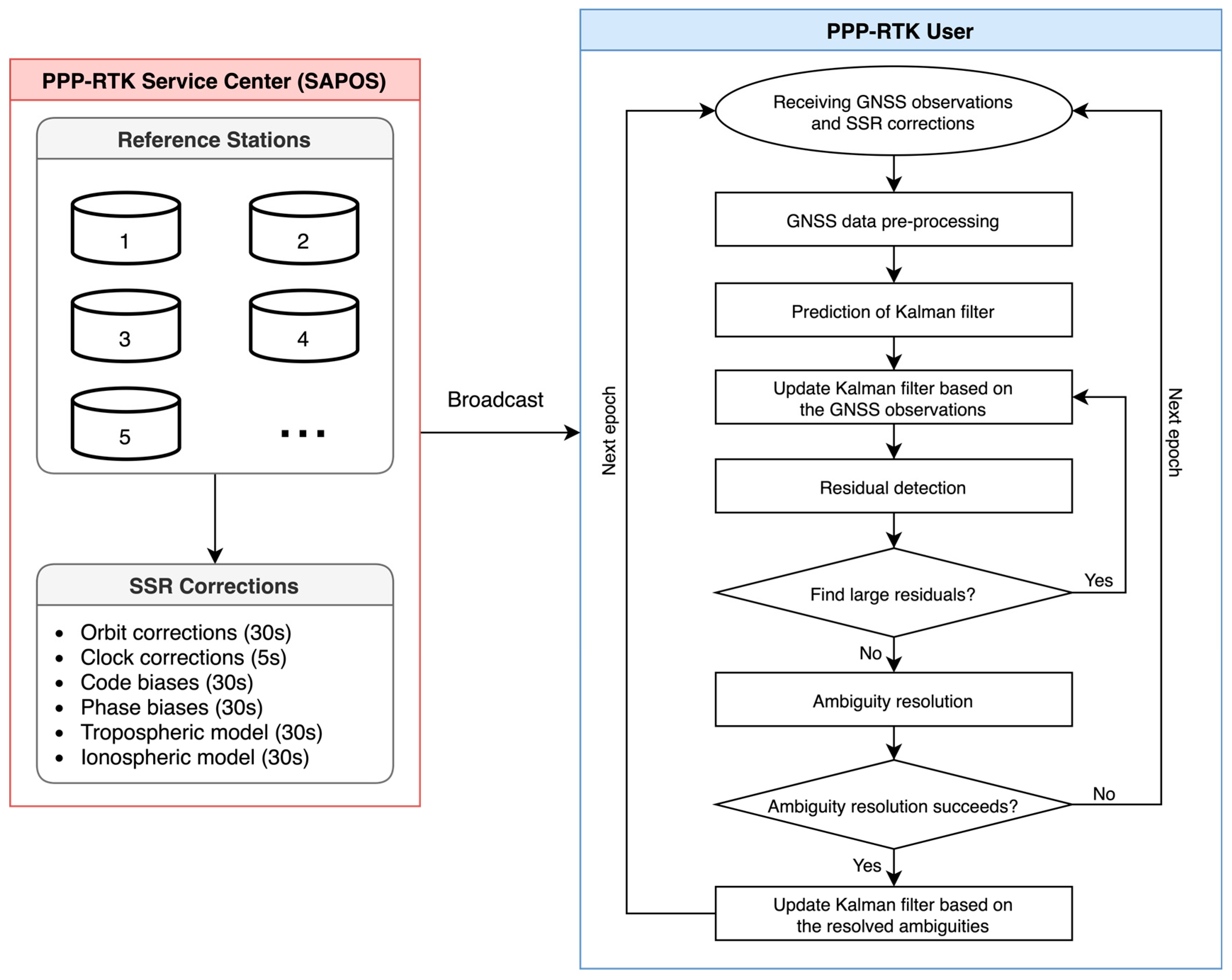
2.1. Workflow

The whole concept of PPP-RTK contains two segments: PPP-RTK service center and PPP-RTK user end, as illustrated in Figure 1. The PPP-RTK service center, e.g., SAPOS in this case, collects GNSS observations from a ground station network which is then used to compute precise satellite orbit and signal biases products with an updating interval of 30 s, the high-rate clock corrections with an interval of 5 s, and simultaneously estimate tropospheric and ionospheric model parameters every 30 s. All of these products are represented as SSR corrections and broadcast to users.

This manuscript will focus on the real-time data processing at the user side which includes the following seven steps as shown in Figure 1:

(1)

Receive GNSS observations and decode SSR corrections in real-time; calculate the SSR tropospheric and ionospheric delays for each satellite based on the approximate position of the receiver;

(2)

GNSS data pre-processing, which mainly removes some potential large errors and detects the cycle slips by using TurboEdit algorithm [31];

(3)

Prediction of Kalman filter based on Section 2.3;

(4)

Update of Kalman filter based on Section 2.4, obtain the PPP-RTK solutions without AR;

(5)

Detect large residuals; if the residual of one satellite is larger than 5 m for code measurements and 0.05 m for phase measurements, or the residual is larger than 3 times of standard deviation of all satellites’ residuals, the satellite will be excluded from the data processing at current epoch. Then, go back to Step (4) and reupdate the state vector of Kalman filter; if there are no large residuals, then go forward to the next step;

(6)

Extract the float ambiguity estimates and their variance-covariance matrix; construct the double-differenced ambiguities between two satellites and two frequency bands to recover the integer feature of the ambiguities, and then resolve the ambiguities to integers; if AR fails, then derive the solutions without AR and proceed to the next epoch, otherwise continue the next step.

(7)

Update the solution of the Kalman filter based on the resolved ambiguities and derive the solutions with AR; finish this epoch and proceed to the next epoch.

2.2. GNSS Observation Equations

GNSS observations equations for code and carrier-phase measurements based on SSR corrections [32] are formulated as

$$\left\{\begin{array}{l}{P}_j^i={\rho }^i+\mathrm{c}\left({dt}_r-{dt}_s\right)+{\delta b}_j-{\delta b}_j^i+m^{i}T+g_j{I}^i++\epsilon \left(P_j^i\right)\\ L_j^i={\rho }^i+\mathrm{c}\left({dt}_r-{dt}_s\right)+{\delta h}_j-{\delta h}_j^i+m^{i}T-{g_{j}I}^i+{\lambda }_j\left(n_j^i+{\delta w}^i\right)+\epsilon \left(L_j^i\right)\\ {SSR}_T^i=m^{i}T+\epsilon \left({SSR}_T^i\right)\\ {SSR}_I^i=I^i+\epsilon \left({SSR}_I^i\right)\end{array}\right.$$

(1)

where $P_j^i$ and $L_j^i$ indicate the code and carrier-phase measurements from satellite $i$ to receiver at frequency $j\left(j=\mathrm{1,2}\right)$; ${\rho }^i$ denotes the distance between the satellite and receiver; ${dt}_r$ and ${dt}_s$ indicate the receiver and satellite clock offsets; ${\delta b}_j$ and ${\delta b}_j^i$ are receiver and satellite code biases; ${\delta h}_j$ and ${\delta h}_j^i$ indicates receiver and satellite phase biases; the Zenith tropospheric delay is marked as $T$ with$m^i$ indicating the global mapping function [33]; The slant ionospheric delay is denoted as $I$, and $g_j={\left(f_j/f_1\right)}^2$ with $f$ meaning the signal frequency; $n_j^i$ represent integer carrier-phase ambiguities and $\lambda$ is the corresponding wavelength; $\epsilon$ means the observation noise. Moreover, the tropospheric and ionospheric delays calculated with SSR corrections are indicated as ${SSR}_T^i$ and ${SSR}_I^i$ [12]. They are treated as pseudo-observations to improve the strength of the PPP-RTK mathematical model. Last but not the least, relativistic effects and satellite carrier-phase windup correction [34] have been corrected in Equation (1). However, in a kinematic scenario, the vehicle may turn at any angular speed and at any time, causing a rotation of the GNSS antenna. As a consequence, the received GNSS carrier-phase measurements will unavoidably contain additional carrier-phase windup effects [35] marked as ${\delta w}^i$ in Equation (1). The receiver carrier-phase biases, ambiguities and windup effects caused by the rotation of receiver antenna are linear correlated with each other, which cannot be estimated separately. Thus, they are combined together and estimated as float ambiguity parameters. Also, the receiver code bias ${\delta b}_j$ will be dumped to the receiver clock parameter, then Equation (1) is simplified as

$$\left\{\begin{array}{l}{P}_j^i={\rho }^i+\mathrm{c}\left({d\tilde{t}}_r-{dt}_s\right)+\delta d_j-{\delta b}_j^i+m^{i}T+g_j{I}^i++\epsilon \left(P_j^i\right)\\ L_j^i={\rho }^i+\mathrm{c}\left({d\tilde{t}}_r-{dt}_s\right)-{\delta h}_j^i+m^{i}T-{g_{j}I}^i+{\lambda }_j{\tilde{n}}_j^i+\epsilon \left(L_j^i\right)\\ {SSR}_T^i=m^{i}T+\epsilon \left({SSR}_T^i\right)\\ {SSR}_I^i=I^i+\epsilon \left({SSR}_I^i\right)\end{array}\right.$$

(2)

with

$$\left\{\begin{array}{c}{\tilde{n}}_1^i=n_1^i+{\delta w}^i+\left({\delta h}_1-{\delta b}_1\right)/{\lambda }_{s,1}\\ {\tilde{n}}_2^i=n_2^i+{\delta w}^i+\left({\delta h}_2-{\delta b}_1\right)/{\lambda }_{s,2}\end{array}\right. \mathrm{and} \left\{\begin{array}{l}{d\tilde{t}}_r={dt}_r+{\delta b}_1\\ \delta d_j={\delta b}_j-{\delta b}_1\end{array}\right.$$

(3)

where $\delta d_j$ means the receiver differential code bias (DCB). The unknown parameters in Equation (2) are classified as three types

$$\left\{\begin{array}{l}\mathit{a}={\left[\begin{array}{cccccc}dx& dy& dz& {d\tilde{t}}_r& {\delta d}_2& T\end{array}\right]}^T\\ {\mathit{b}}^i=\left[I^i\right]\\ {\tilde{\mathit{n}}}^i={\left[\begin{array}{cc}{\tilde{n}}_{s,1}^i& {\tilde{n}}_{s,2}^i\end{array}\right]}^T\end{array}\right.,$$

(4)

Then, the corresponding matrix format of GNSS observation equations from satellite $i$ is derived from Equation (2) as

$${\mathit{Z}}^i=\left[\begin{array}{ccc}{\mathit{H}}_{\mathit{a}}^i& {\mathit{H}}_{\mathit{b}}^i& {\mathit{H}}_{\mathit{n}}^i\end{array}\right]\left[\begin{array}{c}{\mathit{a}}^i\\ {\mathit{b}}^i\\ {\tilde{\mathit{n}}}^i\end{array}\right]+{\mathit{V}}^i={\mathit{H}}^i{\mathit{X}}^i+{\mathit{V}}^i,$$

(5)

in which

$${\mathit{Z}}^i={\left[\begin{array}{cccccc}{P}_1^i& P_2^i& L_1^i& L_2^i& {SSR}_T^i& {SSR}_I^i\end{array}\right]}^T-{\rho }_0^i,$$

(6)

$${\mathit{H}}_{\mathit{a}}^i=\left[\begin{array}{cccccc}\frac{X_0-X_{SSR}^i}{{\rho }_0^i}& \frac{Y_0-Y_{SSR}^i}{{\rho }_0^i}& \frac{Z_0-Z_{SSR}^i}{{\rho }_0^i}& 1& 0& m^i\\ \frac{X_0-X_{SSR}^i}{{\rho }_0^i}& \frac{Y_0-Y_{SSR}^i}{{\rho }_0^i}& \frac{Z_0-Z_{SSR}^i}{{\rho }_0^i}& 1& 1& m^i\\ \frac{X_0-X_{SSR}^i}{{\rho }_0^i}& \frac{Y_0-Y_{SSR}^i}{{\rho }_0^i}& \frac{Z_0-Z_{SSR}^i}{{\rho }_0^i}& 1& 0& m^i\\ \frac{X_0-X_{SSR}^i}{{\rho }_0^i}& \frac{Y_0-Y_{SSR}^i}{{\rho }_0^i}& \frac{Z_0-Z_{SSR}^i}{{\rho }_0^i}& 1& 0& m^i\\ 0& 0& 0& 0& 0& m^i\\ 0& 0& 0& 0& 0& 0\end{array}\right],$$

(7)

where $\left(X_0,Y_0,Z_0\right)$ is the receiver approximate position; $\left(X_{SSR}^i,Y_{SSR}^i,Z_{SSR}^i\right)$ is the precise satellite position, which is calculated from SSR satellite orbit information and ${\rho }_0^i=\sqrt{{\left(X_{SSR}^i-X_0\right)}^2+{\left(Y_{SSR}^i-Y_0\right)}^2+{\left(Z_{SSR}^i-Z_0\right)}^2}$. The submatrix ${\mathit{H}}_{\mathit{b}}^i$ and ${\mathit{H}}_{\mathit{n}}^i$ are expressed as

$${\mathit{H}}_{\mathit{b}}^i={\left[\begin{array}{cccccc}1& g_2& -1& -g_2& 0& 1\end{array}\right]}^T,$$

(8)

$${\mathit{H}}_{\mathit{n}}^i={\left[\begin{array}{cccccc}0& 0& {\lambda }_1& 0& 0& 0\\ 0& 0& 0& {\lambda }_2& 0& 0\end{array}\right]}^T$$

(9)

and

$${\mathit{V}}^i=diag\left[\begin{array}{cccccc}{\epsilon \left(P_1^i\right)}^2& {\epsilon \left(P_2^i\right)}^2& {\epsilon \left(L_1^i\right)}^2& \epsilon {\left(L_2^i\right)}^2& {\epsilon \left({SSR}_T^i\right)}^2& {\epsilon \left({SSR}_I^i\right)}^2\end{array}\right].$$

(10)

Assuming $l$ satellites are observed, then the GNSS observation equation is formulated as

$$\mathit{Z}=\mathit{H}\mathit{X}+\mathit{V},$$

(11)

where,

$$\mathit{Z}=\left[\begin{array}{c}{\mathit{Z}}^1\\ ⋮\\ {\mathit{Z}}^l\end{array}\right],$$

(12)

$$\mathit{H}=\left[\begin{array}{ccccccc}{\mathit{H}}_{\mathit{a}}^1& {\mathit{H}}_{\mathit{b}}^1& \mathbf{0}& \mathbf{0}& {\mathit{H}}_{\mathit{n}}^1& \mathbf{0}& \mathbf{0}\\ ⋮& \mathbf{0}& \ddots & \mathbf{0}& \mathbf{0}& \ddots & \mathbf{0}\\ {\mathit{H}}_{\mathit{a}}^l& \mathbf{0}& \mathbf{0}& {\mathit{H}}_{\mathit{b}}^l& \mathbf{0}& \mathbf{0}& {\mathit{H}}_{\mathit{n}}^l\end{array}\right],$$

(13)

$$\mathit{X}={\left[\begin{array}{ccc}\mathit{a}& \mathit{b}& \tilde{\mathit{n}}\end{array}\right]}^T,\mathit{b}={\left[\begin{array}{ccc}{\mathit{b}}^1& \cdots & {\mathit{b}}^l\end{array}\right]}^T,\tilde{\mathit{n}}={\left[\begin{array}{cccccc}{\tilde{n}}_1^1& \cdots & {\tilde{n}}_1^l& {\tilde{n}}_2^1& \cdots & {\tilde{n}}_2^l\end{array}\right]}^T$$

(14)

and

$$\mathit{V}=diag\left[\begin{array}{ccc}{\mathit{V}}^1& \cdots & {\mathit{V}}^l\end{array}\right],$$

(15)

Therefore, Equation (11) is the basic GNSS observation equation in matrix format, which will be solved by Kalman filter to determine the unknown parameters.

2.3. Prediction of Kalman Filter

Let ${\mathit{X}}_k$ be the state vector at epoch $k$, then the prediction of Kalman filter from epoch $k-1$ to $k$ is described by

$${\mathit{X}}_{k|k-1}={\mathit{F}}_k{\mathit{X}}_{k-1|k-1}+{\mathit{W}}_k,$$

(16)

where ${\mathit{F}}_k$ and ${\mathit{W}}_k$ mean state transition matrix and process noise. ${\mathit{W}}_k$ follows a zero mean multivariate normal distribution with a variance of ${\mathit{Q}}_k$, which is written as

$${\mathit{Q}}_k=\left[\begin{array}{ccc}{\mathit{Q}}_{\mathit{a}}& \mathbf{0}& \mathbf{0}\\ \mathbf{0}& {\mathit{Q}}_{\mathit{b}}& \mathbf{0}\\ \mathbf{0}& \mathbf{0}& {\mathit{Q}}_{\tilde{\mathit{n}}}\end{array}\right].$$

(17)

Assuming the sampling rate is 1 Hz, its values could be set as

$$\left\{\begin{array}{l}{\mathit{Q}}_{\mathit{a}}=\left[\begin{array}{cccc}{5}^2{·\mathit{I}}_{3\times 3}& \mathbf{0}& \mathbf{0}& \mathbf{0}\\ \mathbf{0}& {100}^2& \mathbf{0}& \mathbf{0}\\ \mathbf{0}& \mathbf{0}& {0.001}^2& \mathbf{0}\\ \mathbf{0}& \mathbf{0}& \mathbf{0}& {0.001}^2\end{array}\right]\\ {\mathit{Q}}_{\mathit{b}}={0.01}^2·{\mathit{I}}_{l\times l}\\ {\mathit{Q}}_{\tilde{\mathit{n}}}={0.005}^2·{\mathit{I}}_{2l\times 2l}\end{array}\right.,$$

(18)

in which ${\mathit{I}}_{3\times 3}$, ${\mathit{I}}_{l\times l}$ and ${\mathit{I}}_{2l\times 2l}$ are identity matrix with dimension of $3\times 3$, $l\times l$ and $2l\times 2l$.

In a kinematic scenario, the position of the receiver changes from time to time. At each epoch, we start with a Single Point Positioning (SPP) solution with initial receiver position and clock offset, thus their process noise values are set as 5² and 100² m². Based on the stability analysis of differential code bias ${\delta d}_2$ [36], we set its process noise as 0.001² m²/second. Due to the changing of troposphere is slower than that of ionosphere, their corresponding process noise values are set as 0.001² and 0.01² m² with a sampling rate of 1 Hz. Besides, the float ambiguity estimation contains the differential signal biases between code and carrier-phase measurements. Although the variation in differential signal bias over a short period is usually ignored, its minor change between the epochs is still considered here. Moreover, the estimated float ambiguities still include the additional windup effects caused by the rotation of receiver antenna, which may happen at any time in real-time kinematic applications and needs to be properly considered. Therefore, the process noise of ambiguities is set as 0.005² cycle² instead of zero. According to Equation (16), the variance-covariance information of the predicted state is obtained as

$${\mathit{P}}_{k|k-1}={\mathit{F}}_k{\mathit{P}}_{k-1|k-1}{\mathit{F}}_k^T+{\mathit{Q}}_k,$$

(19)

2.4. Update of Kalman Filter

According to Equation (11), a measurement vector ${\mathit{Z}}_k$ can be formulated as a function of the predicted state ${\mathit{X}}_{k|k-1}$ at epoch k as

$${\mathit{Z}}_k={\mathit{H}}_k{\mathit{X}}_{k|k-1}+{\mathit{V}}_k.$$

(20)

By solving Equation (20), the corrected solution is written as

$${\mathit{X}}_{k|k}={\mathit{X}}_{k|k-1}+{\mathit{K}}_k\left({\mathit{Z}}_k-{\mathit{H}}_k{\mathit{X}}_{k|k-1}\right),$$

(21)

with Kalman gain matrix expressed as ${\mathit{K}}_k$

$${\mathit{K}}_k={\mathit{P}}_{k|k-1}{\mathit{H}}_k^T{\left({\mathit{H}}_k{\mathit{P}}_{k|k-1}{\mathit{H}}_k^T+{\mathit{V}}_k\right)}^{-1}.$$

(22)

The variance-covariance matrix of the solution can be obtained by

$${\mathit{P}}_{k|k}=\left(\mathit{I}-{\mathit{K}}_k{\mathit{H}}_k\right){\mathit{P}}_{k|k-1}=\left[\begin{array}{ccc}{\mathit{P}}_{\mathit{a}\mathit{a}}& {\mathit{P}}_{\mathit{a}\mathit{b}}& {\mathit{P}}_{\mathit{a}\tilde{\mathit{n}}}\\ {\mathit{P}}_{\mathit{b}\mathit{a}}& {\mathit{P}}_{\mathit{b}\mathit{b}}& {\mathit{P}}_{\mathit{b}\tilde{\mathit{n}}}\\ {\mathit{P}}_{\tilde{\mathit{n}}\mathit{a}}& {\mathit{P}}_{\tilde{\mathit{n}}\mathit{b}}& {\mathit{P}}_{\tilde{\mathit{n}}\tilde{\mathit{n}}}\end{array}\right],$$

(23)

where the estimated float ambiguity and its variance-covariance matrix indicated as $\tilde{\mathit{n}}$ and ${\mathit{P}}_{\tilde{\mathit{n}}\tilde{\mathit{n}}}$ are used in the next step for AR.

2.5. Ambiguity Resolution

Due to the contamination of receiver signal biases, the estimated float ambiguities do not have the integer feature. We have to remove the influence of receiver signal biases on ambiguity estimation by differencing the ambiguities between two satellites. Given a pivot satellite, the single-differenced ambiguities are constructed as

$$∆\tilde{\mathit{n}}=\mathit{M}·\tilde{\mathit{n}}=={\left[\begin{array}{c}{∆n}_1^{1,p}+∆{\delta w}^{1,p}\\ ⋮\\ \begin{array}{c}\begin{array}{c}{∆n}_1^{l,p}+{∆\delta w}^{l,p}\\ {∆n}_2^{1,p}+{∆\delta w}^{1,p}\\ \begin{array}{c}⋮\\ \begin{array}{c}{∆n}_2^{l,p}+{∆\delta w}^{l,p}\end{array}\end{array}\end{array}\end{array}\end{array}\right]}_{\left(2l-2\right)\times 1},$$

(24)

where $∆$ means differencing the ambiguity estimates between two satellites and is realized by a matrix $\mathit{M}$. Because of the additional windup effects caused by rotation of receiver antenna in a kinematic scenario, the single-differenced ambiguities $∆\tilde{\mathit{n}}$ in Equation (24) still do not have an integer feature. Considering the additional windup effects on different frequency bands for a specific satellite are identical, we further difference the ambiguities between two frequency bands and construct the ambiguities as

$$\nabla ∆\tilde{\mathit{n}}=\mathit{N}·∆\tilde{\mathit{n}}=\mathit{N}·\mathit{M}·\tilde{\mathit{n}}={\left[\begin{array}{c}\nabla {∆n}_{\mathrm{1,2}}^{1,p}\\ \begin{array}{c}⋮\\ \begin{array}{c}{\nabla ∆n}_{\mathrm{1,2}}^{l,p}\end{array}\end{array}\end{array}\right]}_{\left(l-1\right)\times 1},$$

(25)

where $\nabla$ means differencing the ambiguities between two frequency bands and is realized by a matrix $\mathit{N}$. By now, the new constructed ambiguities $\nabla ∆\tilde{\mathit{n}}$ can be resolved to integers. Their variance-covariance matrix is calculated as

$${\mathbf{Q}}_{\nabla ∆\tilde{\mathit{n}}}=\mathit{N}·\mathit{M}·{\mathit{P}}_{\tilde{\mathit{n}}\tilde{\mathit{n}}}·{\mathit{M}}^{\mathit{T}}·{\mathit{N}}^{\mathit{T}},$$

(26)

$\nabla ∆\tilde{\mathit{n}}$ and ${\mathbf{Q}}_{\nabla ∆\tilde{\mathit{n}}}$ will be seen as two inputs of the Modified Least-squares Ambiguity Decorrelation algorithm (MLAMDA) for AR [37,38]. The fixed failure rate is configured as 1% for ambiguity validation [39]. The successfully resolved ambiguities are denoted as

$$\mathit{E}=MLAMBDA\left(\nabla ∆\tilde{\mathit{n}},{\mathbf{Q}}_{\nabla ∆\tilde{\mathit{n}}}\right),$$

(27)

2.6. Solution with AR

The update equation of the resolved ambiguities in Kalman filter at epoch $k$ is described as

$${\mathit{E}}_k={\check{\mathit{H}}}_k{\mathit{X}}_k+{\check{\mathit{V}}}_k,$$

(28)

The design matrix ${\check{\mathit{H}}}_k$ is described as

$${\check{\mathit{H}}}_k=\left[\begin{array}{ccc}{0}_{\left(l-1\right)\times 6}& 0_{\left(l-1\right)\times l}& \mathit{N}·\mathit{M}\end{array}\right],$$

(29)

${\check{\mathit{V}}}_k$ is the noise of resolved ambiguities and assumed as

$${\check{\mathit{V}}}_k={10}^{-12}·{\mathit{I}}_{\left(l-1\right)\times \left(l-1\right)},$$

(30)

By solving Equation (28), the solution with AR is formulated as

$${\check{\mathit{X}}}_{k|k}={\mathit{X}}_{k|k}+{\check{\mathit{K}}}_k\left({\mathit{E}}_k-{\check{\mathit{H}}}_k{\mathit{X}}_{k|k}\right),$$

(31)

where ${\check{\mathit{K}}}_k$ is the Kalman gain matrix contributed by the resolved ambiguities,

$${\check{\mathit{K}}}_k={\mathit{P}}_{k|k}{\check{\mathit{H}}}_k^T{\left({\check{\mathit{H}}}_k{\mathit{P}}_{k|k}{\check{\mathit{H}}}_k^T+{\check{\mathit{V}}}_k\right)}^{-1},$$

(32)

The corresponding variance-covariance of the solution with AR is written as

$${\check{\mathit{P}}}_{k|k}=\left(\mathit{I}-{\check{\mathit{K}}}_k{\check{\mathit{H}}}_k\right){\mathit{P}}_{k|k},$$

(33)

3. PPP-RTK Performances in a Static Scenario

3.1. Data Collection and Processing Strategies

To validate the PPP-RTK performances in a static scenario, we installed a JAVAD GNSS receiver on the roof of a building at the Institute of Communications and Navigation, German Aerospace Center (DLR), and collected data for 5 days from the 15th to 19th of April in 2022 with a sampling rate of 1 Hz. Meanwhile, we received the SAPOS SSR corrections through internet in real-time. The real-time SSR corrections include three parts: (1) low rate SSR corrections with a time update rate of 30 s, containing satellite orbit, clock and signal biases, (2) high-rate satellite clock corrections updated every 5 s, and (3) atmospheric products updated every 30 s. These SSR corrections were determined by SAPOS based on 19 reference stations distributed in southern Bavaria which are indicated as black dots in Figure 2.

Table 1. Data processing strategies of PPP-RTK.

Item	PPP-RTK Processing Strategies
Processing mode	Kinematic mode in real-time
GNSS and frequency band	GPS L1 + L2 and Galileo E1 + E5a code and phase measurements
Observation noise	0.6 m for code measurements and 0.01 cycles for carrier-phase measurements; 0.01 m for SSR tropospheric corrections and 0.05 m for ionospheric corrections
Weighting strategy	Equal weight factor for GPS and Galileo measurements and weight factor is defined as: $\left\{\begin{array}{l}1, elevation>{30}^{°}\\ \frac{1}{2\sin \left(elevation\right)}, elevation \le {30}^{°}\end{array}\right.$
Elevation mask	15°
Ambiguities	Resolved by full and partial MLAMBDA algorithm epoch by epoch and set fix failure rate as 1%
Satellite orbit, clock and biases	Real-time SSR corrections: (1) satellite orbit, clock and signal bias corrections updated every 30 s; (2) high-rate clock correction with an updating interval of 5 s
Atmospheric delay	Corrected with SSR corrections and estimated with other parameters

lists the data processing strategies of PPP-RTK. The data were processed by RTFramework [40], which is designed and developed for real-time GNSS data processing with SSR corrections. It records the time tag plus the real-time raw data-stream of GNSS observations and SSR corrections, which can be used to repeat the real-time scenario of GNSS data processing after the measurement campaign. The average position of daily solutions is seen as the reference position and used to evaluate PPP-RTK performances.

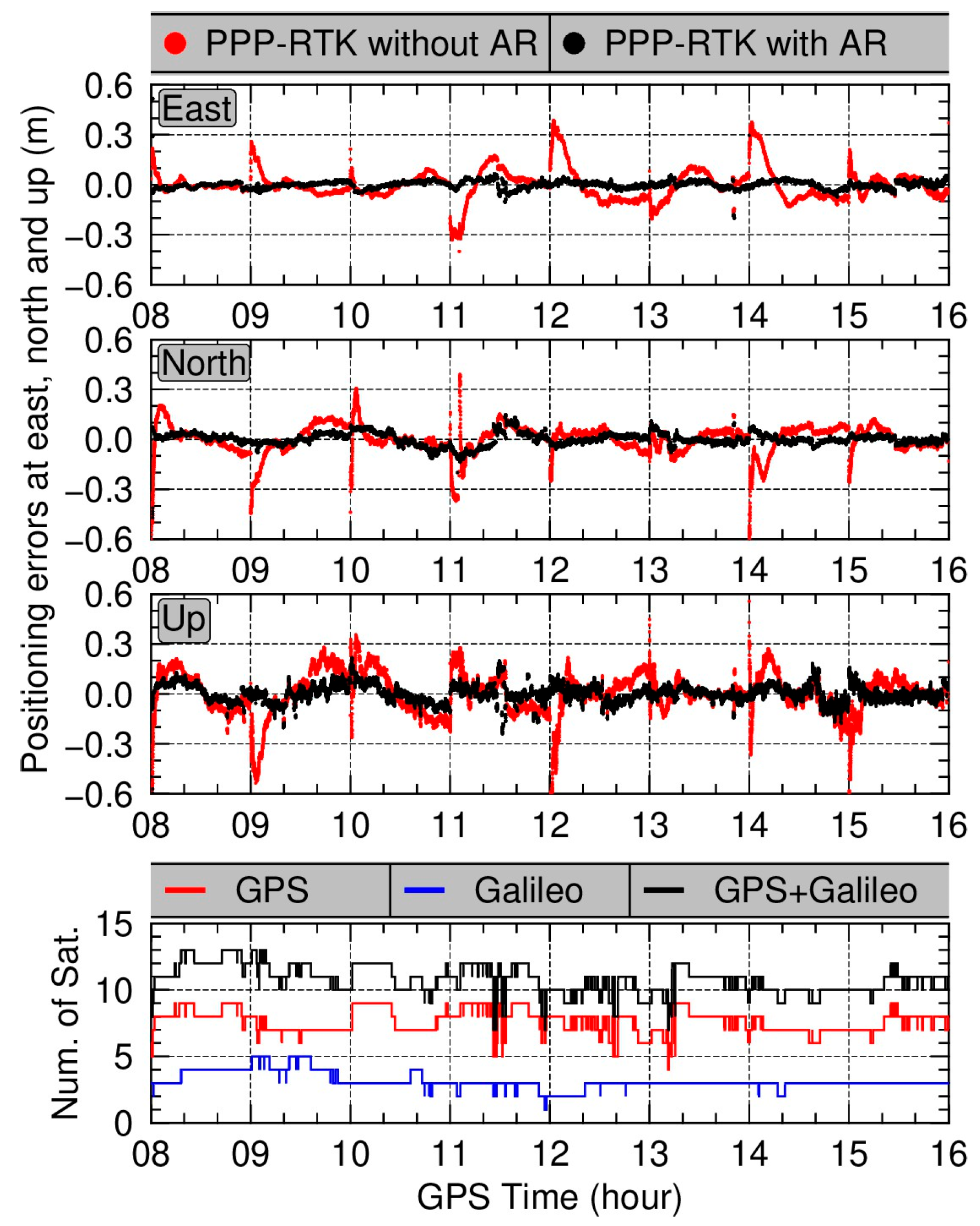
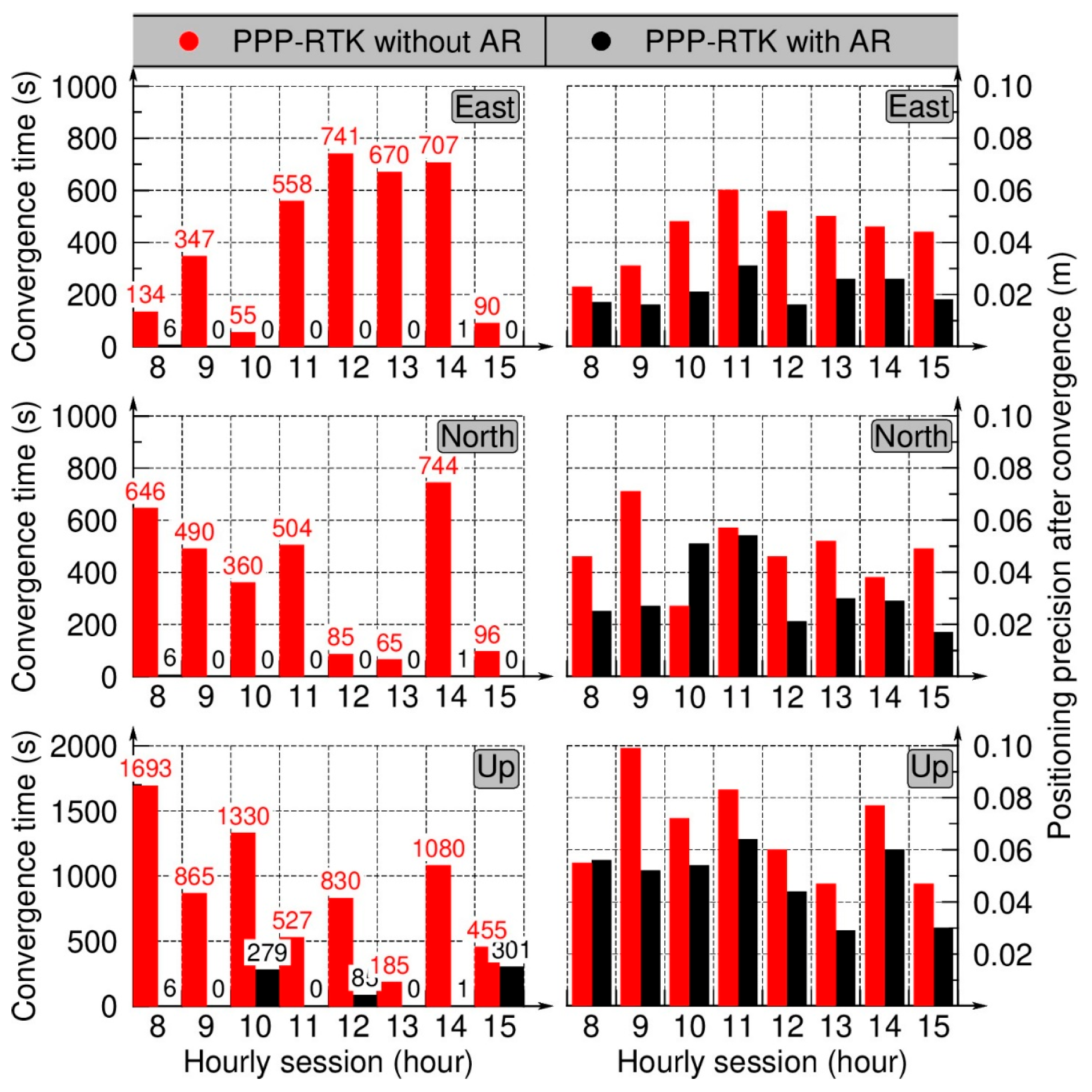
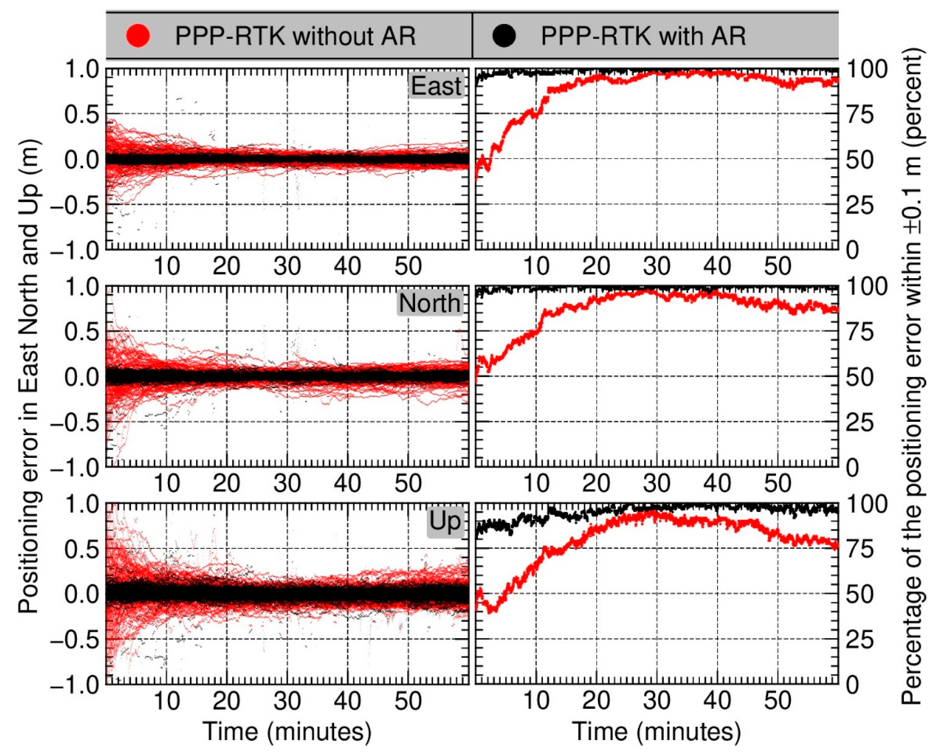
3.2. Positioning Precision and Convergence Time

The data were processed in a simulated real-time kinematic mode. Typically, the activity of ionosphere in one day affects the PPP-RTK performance, and the ionosphere is most active at 14:00 in local time [41]. Therefore, as an example, the PPP-RTK positioning errors from local time 10:00 to 18:00 (GPS time 08:00 to 16:00) in the middle day (17 April) of the measurement campaign are illustrated in Figure 3. The PPP-RTK solver was reset and initialized at each hour to investigate the convergence time. As a comparison, the PPP-RTK results without AR are also shown. The positioning errors of the PPP-RTK without AR scheme in the east, north, and up directions are unstable especially at times from 10:00 to 14:00. This is caused by the high ionospheric activities during this time, and it can be seen from Figure 4, which presents the corresponding time series of vertical Total Electron Content (TEC) of ionosphere at this station. The vertical TEC values are calculated based on the global ionosphere maps from the Center for Orbit Determination in Europe (CODE), and they are higher than 200 from 10:00 to 14:00 which consequently affects the PPP-RTK performances.

In this case, the convergence time is defined as the positioning errors start to be within ±0.1 m and remain within ±0.1 m in the sequential 180 epochs (3 min). The PPP-RTK convergence time and its positioning precision (one sigma) after convergence are presented in Figure 5. From Figure 3 and Figure 5, we can see the PPP-RTK without AR need several to ten minutes to achieve convergence in horizontal and even more than 20 min in vertical component. However, the AR significantly reduces the convergence time. Most of the ambiguities are resolved successfully at the first epoch and then derive precise solutions. The fixing rate of ambiguities is 99.4% on average. The lowest fixing rate among the 8 sessions is 96.6%. For most of the hourly sessions, the convergence time is zero second in horizontal, and in the north component the longest convergence time is 6 s for the session starting at 8:00. Even for the up component, 5 of 8 sessions achieved a rapid convergence of less than 6 s. After the convergence, the PPP-RTK solutions with AR typically have a higher precision than those without AR. The precision (one sigma) of the solutions in the east, north and up components are 0.044 m, 0.048 m and 0.068 m without AR, which are improved to 0.021 m, 0.032 m and 0.049 m for the solutions with AR. The session from 11:00 to 12:00 has a relatively low positioning precision after convergence. This is because only five GPS satellites are available with SSR corrections for several minutes in this session, thus the corresponding positioning errors during this time are relatively larger.

This measurement campaign collected five days of data, which totally contains 120 hourly sessions and 3600 epochs per session. To clearly see the trend of positioning errors, the positioning errors of the 120 hourly sessions overlapped together with the x-axis indicating the seconds of each hour, as presented on the left panels of Figure 6. For every second, there are in principle 120 PPP-RTK results from the 120 hourly sessions. The corresponding percentage of positioning errors within ±0.1 m at each second is presented on the right panels of Figure 6, and for the solutions without AR it takes 843, 883 and 1315 s on east, north and up components when the percentages reach up to 90%. However, for the solutions with AR, 94.1% (113 sessions) of the 120 sessions successfully resolved the ambiguity at the first epoch. Meanwhile, at the first epoch 89.1% (107 sessions) and 92.5% (111 sessions) of the 120 sessions have positioning errors less than 10 cm in the east and north directions. As for the up component, the convergence time is longer than that in horizontal. As a summary, using the SSR corrections generated based on a local GNSS network, more than 90% of the PPP-RTK sessions can realize an instant AR and achieve a rapid convergence in horizontal within few seconds.

4. Real-Time PPP-RTK Applications for Vehicle Transportation

In the applications of vehicle transportation, people are more interested in the performance of PPP-RTK in horizontal components than the vertical component. Thus, the positioning performances in horizontal are mainly analyzed. This section names the solutions with successful AR as fixed solution, otherwise float solutions. First, it introduces the measurement campaign on highway; Second, it evaluates the horizontal positioning performances, then presents statistics of the time required to achieve AR and convergence.

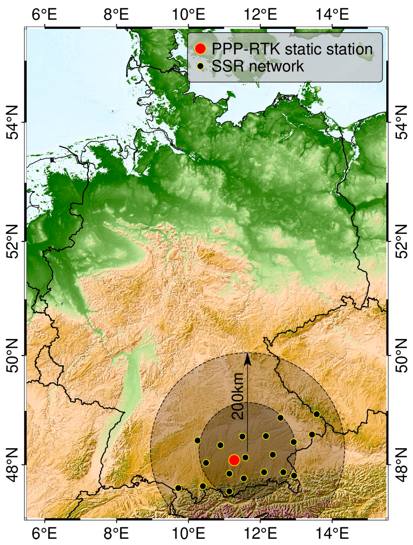
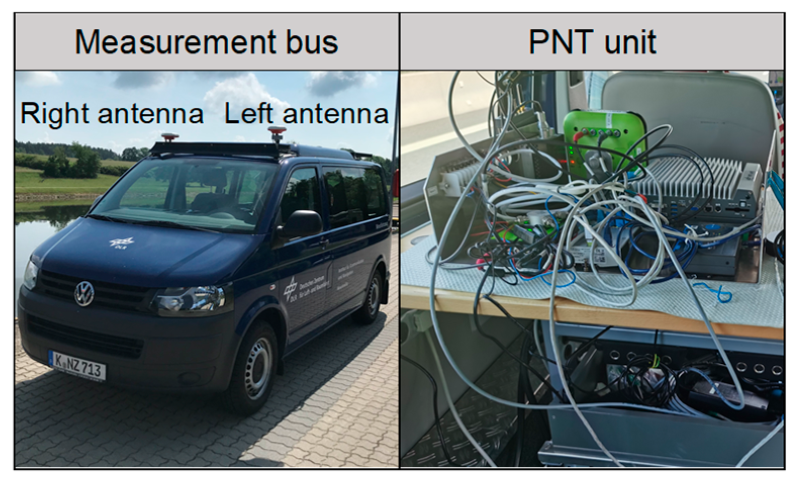
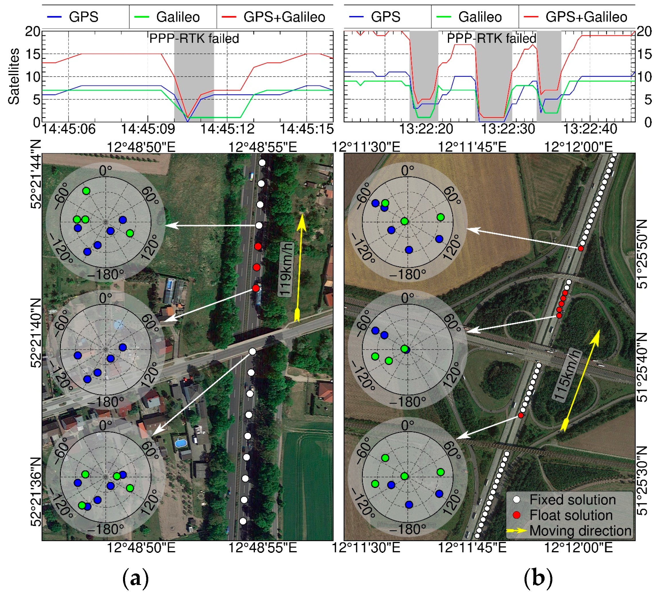
4.1. Measurement Campaign

The measurement bus and Positioning, Navigation and Timing (PNT) unit are shown in Figure 7. Two geodetic GNSS antennas, named as left and right antennas, were mounted on the bus and connected with a JAVAD Delta and a JAVAD Triumph receiver, respectively. The PNT unit was installed inside the car and responsible for decoding the received SSR corrections and computing PPP-RTK solutions in real-time. The SAPOS SSR corrections were determined based on a network of 19 reference stations distributed in northern Bavaria, as shown in Figure 8. The measurement campaign was carried out on 30 June 2021 from Hilpoltstein to Berlin in Germany.

The data processing strategies of PPP-RTK refer to Table 1. To evaluate and analyze the PPP-RTK performances, as a reference, we calculated RTK solutions of the rover receiver based on four RTK base stations shown in Figure 8. Among the four RTK base stations, HILP is a base station at the starting point in Hilpoltstein. HOFJ is chosen from EUREF Permanent GNSS Network (EPN) and LEIJ, POTS are both from International GNSS Service (IGS) stations. RTK typically requires the baseline length between rover receiver and base station not being longer than 20 km. Therefore, the RTK solutions are restricted to a distance within 20 km of the RTK base stations. The RTK reference solutions are computed by RTKLib [42] in a post-processing mode with the processing strategies presented in

Table 2. Processing strategies of RTK.

Item	RTK Processing Strategies
Processing mode	Kinematic mode in post-processing
GNSS and frequency band	GPS L1 + L2 and Galileo E1 + E5a code and phase measurements
Observation noise	The ratio between code and carrier-phase measurements is 100
Weighting strategy	Elevation dependent:$a+\frac{b}{\sin \left(elev\right)}$, where $a=0.002$, $b=0.002$
Elevation mask	15°
Ambiguities	Use LAMBDA resolving the ambiguities with a ratio test of 2.0
Satellite orbit, clock, biases	Final orbit and clock products from CODE, the signal biases are eliminated in double differenced observations
Atmospheric delay	Significantly reduced and ignored in double differenced observations

. Taking the left antenna as an example, the PPP-RTK solutions are compared with the RTK solutions in following.

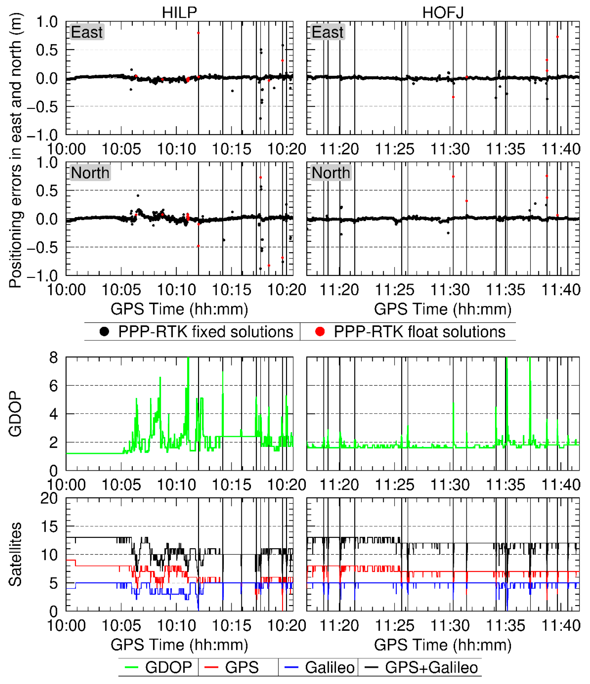
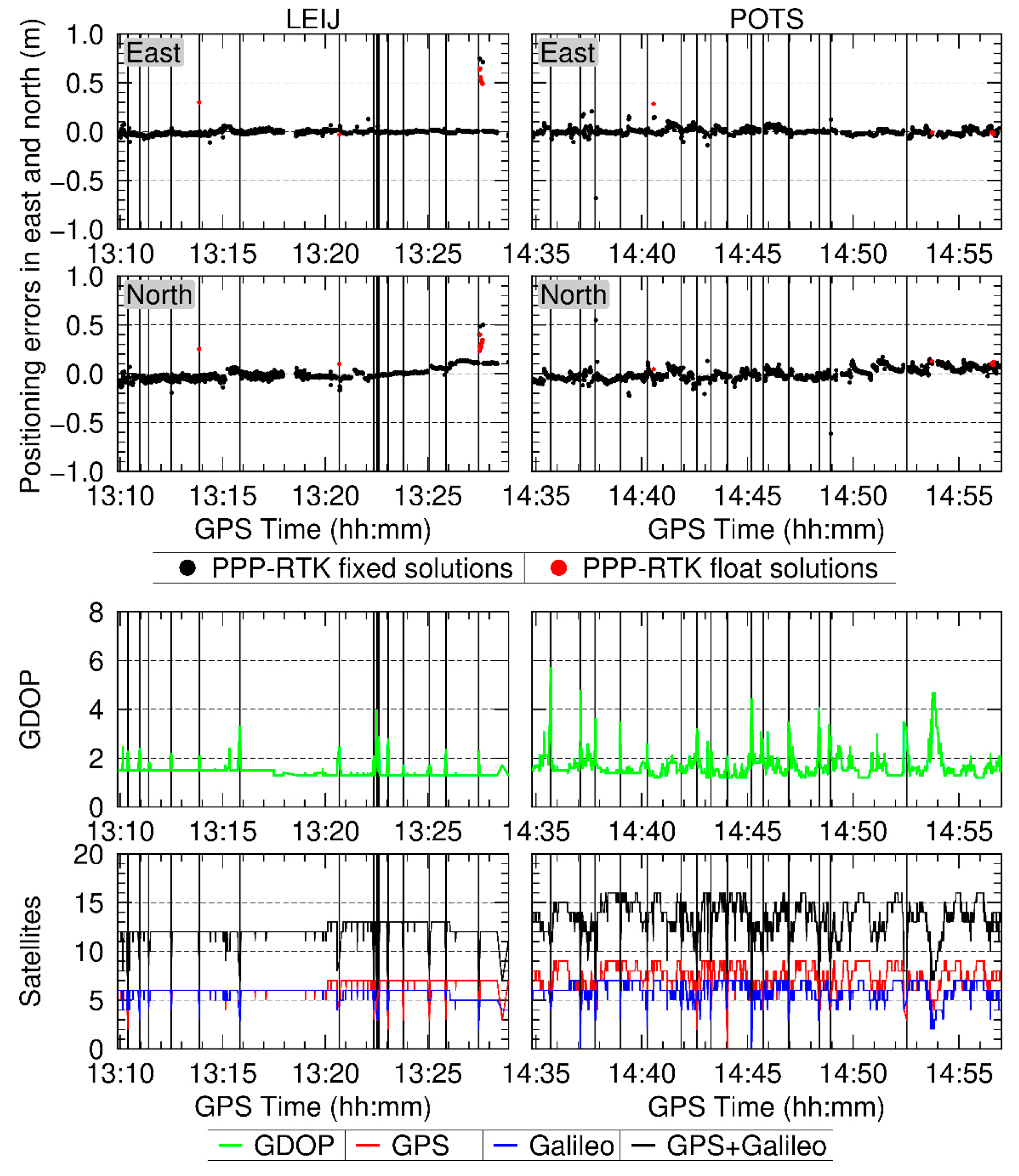
4.2. Positioning Precision

The positioning errors of PPP-RTK with respect to RTK solutions for the two sessions of HILP and HOFJ are plotted in Figure 9. The corresponding Geometric Dilution of Precision (GDOP) values and available satellites are illustrated in the panels of the third and fourth rows of Figure 9. From 10:00:00 to 10:04:35 the bus was in a static mode, the positioning errors in the north and east are lower than 0.1 m. The bus departed at 10:04:35 and drove on the local road from 10:04:35 to the time of passing through the first bridge at 10:12:00. There are a lot of trees on each side of the local road, where only satellites with an elevation higher than 30 degrees are available, as illustrated in Figure 10, and only 6 GPS and 3 Galileo satellites were available. Limited by the available satellites and affected by the trees alongside the local road, the positioning errors were larger than 10 cm especially in the north component from 10:04:25 to 10:12:00. From then on, the bus drove on the highway. The satellite visibility of the receiver on the highway is better than that on the local road. The standard deviations of positioning errors in east and north are 0.129 m and 0.171 m during session HILP, and they are 0.033 m and 0.058 m during session HOFJ. The PPP-RTK performance in session HOFJ is better than that in session HILP, because the satellite visibility of the receiver in session HOFJ is better than that in session HILP. Only 55.9% of the GDOP values are lower than 2 for the session HILP, while it is 93.3% for session HOFJ. The bus passed through many bridges on the highway. Because the GNSS signals are interrupted by the bridges, the positioning errors are becoming large just before and after the bridge passages.

The positioning errors of PPP-RTK compared with RTK solutions for the two sessions of LEIJ and POTS are shown in Figure 11. Because the regions of LEIJ and POTS are roughly 100 km and 200 km away from the coverage of SSR network as plotted in Figure 8, the standard deviations of the positioning errors for the two sessions LEIJ and POTS are higher than that of session HOFJ. The standard deviations in east and north components are 0.070 m and 0.081 m for session LEIJ, and they are 0.055 m and 0.078 m for session POTS. This proves that, even though the application area is far away from the coverage of GNSS network, the SSR corrections can still be well applied for a high-precision PPP-RTK. By observing the GDOP values on the highway for the sessions LEIJ and POTS in Figure 11 and HOFJ and HILP (from 10:12:00 to 10:20:36) in Figure 9, we can observe the GDOP values are normally lower than two, except for the time when passing through bridges, and the positioning errors are large when the GDOP values are high, especially during the bus passing through a bridge. Following this, the PPP-RTK convergence after each bridge passage will be assessed.

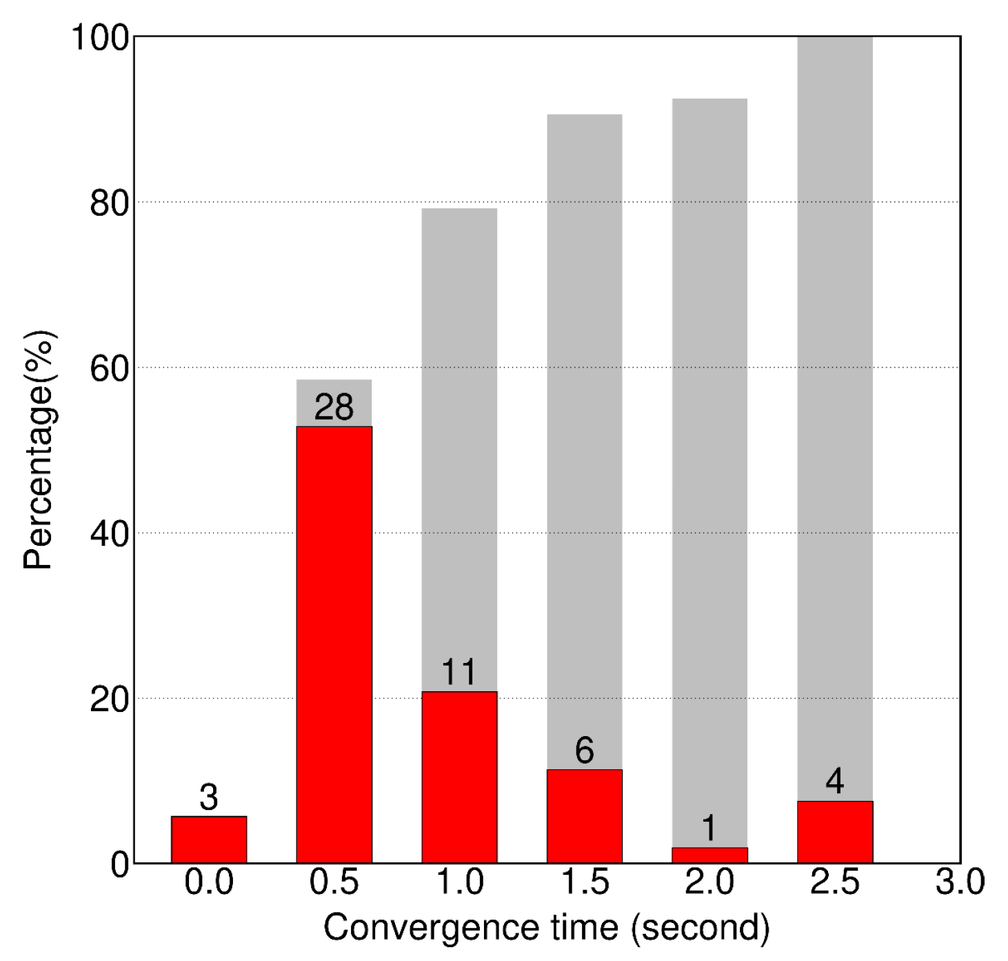
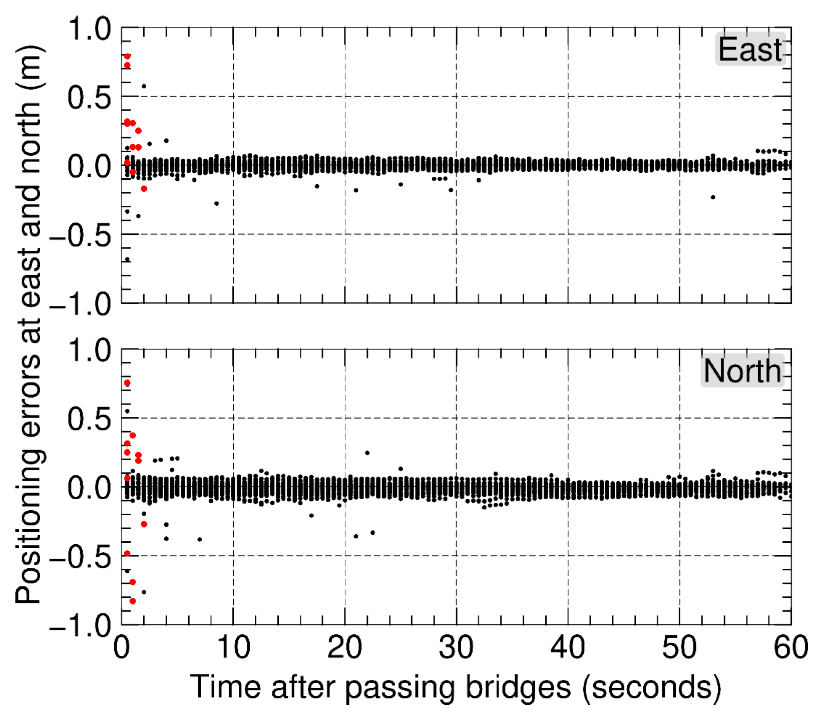
4.3. Convergence Time

Normal and complicated scenarios of PPP-RTK solutions over the bridge passages are shown in Figure 12. In the normal scenario, the GNSS signals were mostly interrupted when the bus was under a bridge. After the bridge passage, the GNSS signals were still affected by the bridge within a short moment, only five GPS satellites and one Galileo satellite were observed. Because one Galileo satellite cannot construct the single-differenced ambiguities between two satellites, consequently one Galileo satellite does not contribute to the PPP-RTK solutions. Thus, only five GPS satellites were available in the sky-plot of the first epoch after the bridge passage. Due to poor satellite visibility of the vehicle, AR failed in the three epochs after the bridge passage. Until the fourth epoch, the satellite visibility of the vehicle became better because of more available Galileo satellites, and PPP-RTK fixed solutions were obtained. With regard to the complicated scenario in Figure 12, the bus passed through three bridges consecutively within a short time. After the first and third bridge passages, the receiver took 1 or 2 s to re-track the satellites. Then, there were more than seven available satellites, and AR succeeded after one float solution. However, there were five float solutions during the second passage. This is because satellite visibility of the vehicle for the second passage is worse than those of the first and third passages, which can be seen from the sky-plots of the three passages in the right subplot of Figure 12. Therefore, after passing bridges the satellite visibility and available satellites affect the time of achieving AR.

In the four sessions of HILP, HOFJ, LEIJ and POTS, the bus crossed 53 bridges in total. The time statistics of achieving AR after these bridge passages are shown in Figure 13. The time interval of PPP-RTK solutions in this kinematic scenario is 0.5 s, and 3 of 53 (5.7%) cases realized AR immediately. Following this, 31 cases (58.5%) obtained the PPP-RTK fixed solutions with 0.5 s, and 48 cases (90.6%) achieved AR within 2 s. Only 1 case took longer than 2.5 s to achieve AR.

The overlapped positioning errors of maximum 60 s after each bridge passage are plotted in Figure 14. For the cases that the bus passed through more than 1 bridge within 60 s, for example in the right subplot of Figure 12, only the positioning errors of 5 s (10 epochs) after the first bridge passage and 3.5 s (7 epochs) after the second bridge passage were considered in Figure 14. The PPP-RTK solutions are usually interrupted and initialized again after crossing the bridges. Thus, at the beginning of bridge passages, there were some float solutions with large errors. PPP-RTK rapidly realized AR within 1 s in 79.3% of the cases. Affected by the traffic signs, trees and some other infrastructures on the highway, some jump errors are also observed in Figure 14.

In our approach, PPP-RTK starts to derive solutions when there are at least six available GPS and Galileo satellites or five GPS satellites if only GPS is available. The bus may pass through several bridges within 3 min in kinematic scenarios, which can be seen from Figure 9 and Figure 11. Thus, the convergence time after a bridge passage in this section is defined as the positioning errors start to be within ±0.1 m and remain within ±0.1 m in the sequential 5 epochs (2.5 s) instead of 180 epochs (3 min), as we defined in Section 3. There are several cases where the epochs with available PPP-RTK solutions between two bridges passage are less than 20 (10 s). For example, in the right subplot of Figure 12, the number of epochs with available PPP-RTK solutions between the first and second bridge is 10 (5 s), and between the second and third bridge is 7 (3.5 s). Because the time is too short, these cases are ignored in the statistical analysis of the convergence time and 3 of the 53 cases are excluded in total. The statistics of convergence time after 50 bridge passages are plotted in Figure 15. Among the 50 cases, the PPP-RTK realized convergence immediately in 2 cases. In 38 of 50 cases, the PPP-RTK convergence time in east and north components is within 2 s. In 92% (46/50) and 94% (47/50) of the cases, PPP-RTK converged within 5 s in the east and north components, respectively. There are only 2 cases with convergence times longer than 10 s.

5. Conclusions and Outlooks

With the support of real-time SSR corrections provided by SAPOS, we developed a PPP-RTK approach, which resolves the double-differenced ambiguities between satellites and frequency bands to integers, realizing PPP-RTK with instant AR and rapid convergence of several seconds. The PPP-RTK performances are evaluated under different scenarios. In an open area of a static scenario, more than 90% of PPP-RTK solutions can realize an instant AR and achieve precise positioning (less than 0.1 m) in horizontal within 2 s. In a kinematic scenario of vehicle transportation, the PPP-RTK performances on the highway are mainly analyzed. The positioning precision on the highway are normally better than 0.1 m except for the time of passing bridges, because the PPP-RTK solver will be interrupted by several seconds and initialize again. After the bridge passages, more than 90% of the cases realized AR within 2 s. We analyzed the PPP-RTK convergence over 50 bridge passages. It showed that 92% and 94% of the cases achieved PPP-RTK convergence within 5 s in the east and north directions, respectively. PPP-RTK with a precision of 0.1 m and rapid convergence of several seconds benefits the precise navigation in transportation, which will support the development of autonomous driving in the future.

Considering the complexities of precise navigation in real-time kinematic scenarios, PPP-RTK is still facing many challenges:

• Continuity: GNSS provides continuous positioning information in an open area but faces challenges in confined scenarios under bridges and in urban areas. Close-range sensors, such as LiDAR/RADAR, work perfectly in these confined scenarios, but faces challenges in an open area where no clear boundaries of infrastructures are visible. In addition, IMU is an independent sensor which provides precise navigation information within a short time when GNSS is unavailable. Therefore, the complementary use of GNSS, close-range sensors and IMU will definitely enhance the capability of continuous navigation in harsh environments.
• Reliability: GNSS signals are susceptible to interference in harsh environments. On one hand, limited by satellite visibility, the PPP-RTK solutions are unreliable. Thus, multi-constellation GNSS PPP-RTK is necessary. On the other hand, multipath signals are unavoidable and affect the reliability of the PPP-RTK. Overcoming multipath effects in harsh environments still needs further research.
• Integrity: real-time PPP-RTK applied for autonomous driving is a safety and liability critical application. Thus, the rigorous integrity concept of the GNSS PPP-RTK is definitely required. But the integrity monitoring algorithms developed in the aviation domain cannot be transported directly into autonomous driving applications. The modified integrity monitoring algorithm for GNSS PPP-RTK needs to be investigated.

References

1. Report on Road User Needs and Requirements: Outcome of the EUSPA User Consultation Platform Issue/Rev: 3.0. 2021. Available online: https://www.gsc-europa.eu/sites/default/files/sites/all/files/Report_on_User_Needs_and_Requirements_Road.pdf (accessed on 1 September 2021).
2. Malys, S.; Jensen, P.A. Geodetic Point Positioning with GPS Carrier Beat Phase Data from the CASA UNO Experiment. Geophys. Res. Lett. 1990, 17, 651–654. [Google Scholar] [CrossRef]
3. Zumberge, J.F.; Heflin, M.B.; Jefferson, D.C.; Watkins, M.M.; Webb, F.H. Precise point positioning for the efficient and robust analysis of GPS data from large networks. J. Geophys. Res. 1997, 102, 5005–5017. [Google Scholar] [CrossRef]
4. Teunissen, P.J.G.; Odolinski, R.; Odijk, D. Instantaneous BeiDou+ GPS RTK positioning with high cut-off elevation angles. J. Geod. 2014, 88, 335–350. [Google Scholar] [CrossRef]
5. Xi, R.; Jiang, W.; Meng, X.; Chen, H.; Chen, Q. Bridge monitoring using BDS-RTK and GPS-RTK techniques. Measurement 2018, 120, 128–139. [Google Scholar] [CrossRef]
6. Kouba, J.; Héroux, P. Precise point positioning using IGS orbit and clock products. GPS Solut. 2001, 5, 12–28. [Google Scholar] [CrossRef]
7. Gao, Y.; Chen, K. Performance analysis of precise point positioning using real-time orbit and clock products. J. Glob. Position. Syst. 2004, 3, 95–100. [Google Scholar] [CrossRef]
8. Li, X.; Zhang, X.; Ge, M. Regional reference network augmented precise point positioning for instantaneous ambiguity resolution. J. Geod. 2011, 85, 151–158. [Google Scholar] [CrossRef]
9. Lou, Y.; Zheng, F.; Gu, S.; Wang, C.; Guo, H.; Feng, Y. Multi-GNSS precise point positioning with raw single-frequency and dual-frequency measurement models. GPS Solut. 2016, 20, 849–862. [Google Scholar] [CrossRef]
10. An, X.; Meng, X.; Jiang, W. Multi-constellation GNSS precise point positioning with multi-frequency raw observations and dual-frequency observations of ionospheric-free linear combination. Satell. Navig. 2020, 1, 7. [Google Scholar] [CrossRef]
11. Wübbena, G.; Schmitz, M.; Bagge, A. PPP-RTK: Precise point positioning using state-space representation in RTK networks. In Proceedings of the ION GNSS 18th International Technical Meeting of the Satellite Division, Long Beach, CA, USA, 13–16 September 2005. [Google Scholar]
12. Wübbena, G.; Perschke, C.; Wübbena, J.; Wübbena, T.; Schmitz, M. GNSS SSR real-time correction: The Geo++ SSRZ format and applications. In Proceedings of the 33rd International Technical Meeting of the Satellite Division of The Institute of Navigation (ION GNSS+ 2020), Virtual, 21–25 September 2020. [Google Scholar] [CrossRef]
13. Mervart, L.; Lukes, Z.; Rocken, C.; Iwabuchi, T. Precise point positioning with ambiguity resolution in real-time. In Proceedings of the ION GNSS, Savannah, GA, USA, 16–19 September 2008. [Google Scholar]
14. Teunissen, P.J.G.; Odijk, D.; Zhang, B. PPP-RTK: Results of CORS network-based PPP with integer ambiguity resolution. J. Aeronaut. Astronaut. Aviat. 2010, 42, 223–229. [Google Scholar]
15. Teunissen, P.J.G.; Khodabandeh, A. Review and principles of PPP-RTK methods. J. Geod. 2015, 89, 217–240. [Google Scholar] [CrossRef]
16. de Jonge, P.J. A Processing Strategy for the Application of the GPS in Networks. Ph.D. Thesis, Delft University of Technology, Delft, The Netherlands, 1998. [Google Scholar]
17. Laurichesse, D.; Mercier, F.; Berthias, J.; Broca, P.; Cerri, L. Integer Ambiguity Resolution on Undifferenced GPS Phase Measurements and Its Application to PPP and Satellite Precise Orbit Determination. Navigation 2009, 56, 135–149. [Google Scholar] [CrossRef]
18. Collins, P.; Lahaye, F.; Herous, P.; Bisnath, S. Precise point positioning with ambiguity resolution using the decoupled clock model. In Proceedings of the ION GNSS 2008, Savannah, GA, USA, 16–19 September 2008. [Google Scholar]
19. Ge, M.; Gendt, G.; Rothacher, M.; Shi, C.; Liu, J. Resolution of GPS carrier-phase ambiguities in precise point positioning (PPP) with daily observations. J. Geod. 2008, 82, 389–399. [Google Scholar] [CrossRef]
20. Laurichesse, D.; Mercier, F.; Berthias, J.; Bijac, J.; Cerri, L. Real time zero-difference ambiguities blocking and absolute RTK. In Proceedings of the ION NTM-2008, San Diego, CA, USA, 28–30 January 2008. [Google Scholar]
21. Geng, J.; Guo, J.; Meng, X.; Gao, K. Speeding up PPP ambiguity resolution using triple-frequency GPS/BeiDou/Galileo/QZSS data. J. Geod. 2020, 94, 6. [Google Scholar] [CrossRef]
22. Nadarajah, N.; Khodabandeh, A.; Wang, K.; Choudhury, M.; Teunissen, P.J.G. Multi-GNSS PPP-RTK: From large-to small-scale networks. Sensors 2018, 18, 1078. [Google Scholar] [CrossRef]
23. Geng, J.; Guo, J.; Chang, H.; Li, X. Towards global instantaneous decimeter-level positioning using tightly-coupled multi-constellation and multi-frequency GNSS. J. Geod. 2018, 93, 977–991. [Google Scholar] [CrossRef]
24. Li, P.; Jiang, X.; Zhang, X.; Ge, M.; Schuh, H. GPS + Galileo + BeiDou precise point positioning with triple-frequency ambiguity resolution. GPS Solut. 2020, 24, 78. [Google Scholar] [CrossRef]
25. Banville, S.; Collins, P.; Zhang, W.; Langley, R.B. Global and regional ionospheric corrections for faster PPP convergence. Navigation 2014, 61, 115–124. [Google Scholar] [CrossRef]
26. Psychas, D.; Verhagen, S.; Liu, X.; Memarzadeh, Y.; Visser, H. Assessment of ionospheric corrections for PPP–RTK using regional ionosphere modelling. Meas. Sci. Technol. 2018, 30, 014001. [Google Scholar] [CrossRef]
27. Yan, Z.; Zhang, X. Assessment of the performance of GPS/Galileo PPP-RTK convergence using ionospheric corrections from networks with different scales. Earth Planets Space 2022, 74, 47. [Google Scholar] [CrossRef]
28. Psychas, D.; Teunissen, P.J.G.; Verhagen, S. A Multi-Frequency Galileo PPP-RTK Convergence Analysis with an Emphasis on the Role of Frequency Spacing. Remote Sens. 2021, 13, 3077. [Google Scholar] [CrossRef]
29. Geng, J.; Teferle, F.N.; Meng, X.; Dodson, A.H. Towards PPP-RTK: Ambiguity resolution in real-time precise point positioning. Adv. Space Res. 2011, 47, 1664–1673. [Google Scholar] [CrossRef]
30. Li, X.; Zhang, X.; Guo, F. Predicting atmospheric delays for rapid ambiguity resolution in precise point positioning. Adv. Space Res. 2014, 54, 840–850. [Google Scholar] [CrossRef]
31. Blewitt, G. An automatic editing algorithm for GPS data. Geophys. Res. Lett. 1990, 17, 199–202. [Google Scholar] [CrossRef]
32. Wang, F.; Geng, J. GNSS PPP-RTK tightly coupled with low-cost visual-inertial odometry aiming at urban canyons. J. Geod. 2023, 97, 66. [Google Scholar] [CrossRef]
33. Böhm, J.; Niell, A.; Tregoning, P.; Schuh, H. Global mapping function (GMF): A new empirical mapping function based on numerical weather model data. Geophys. Res. Lett. 2006, 33, L07304. [Google Scholar] [CrossRef]
34. Wu, J.T.; Wu, S.C.; Hajj, G.; Bertiger, W.I.; Lichten, S.M. Effects of antenna orientation on GPS carrier phase. Manuscr. Geod. 1993, 18, 91–98. [Google Scholar]
35. Banville, S.; Tang, H. Antenna rotation and its effects on kinematic Precise point positioning. In Proceedings of the ION GNSS 2010, Institute of Navigation, Portland, OR, USA, 21–24 September 2010. [Google Scholar]
36. Li, M.; Yuan, Y.; Wang, N.; Liu, T.; Chen, Y. Estimation and analysis of the short-term variations of multi-GNSS receiver differential code biases using global ionosphere maps. J. Geod. 2018, 92, 889–903. [Google Scholar] [CrossRef]
37. Chang, X.W.; Yang, X.; Zhou, T. MLAMBDA: A modified LAMBDA method for integer least-squares estimation. J. Geod. 2005, 79, 552–565. [Google Scholar] [CrossRef]
38. Teunissen, P.J.G. The least-squares ambiguity decorrelation adjustment: A method for fast GPS integer ambiguity estimation. J. Geod. 1995, 70, 65–82. [Google Scholar] [CrossRef]
39. Verhagen, S.; Teunissen, P.J.G. The ratio test for future GNSS ambiguity resolution. GPS Solut. 2013, 17, 535–548. [Google Scholar] [CrossRef]
40. Gewies, S.; Becker, C.; Noack, T. Deterministic framework for parallel real-time processing in GNSS applications. In Proceedings of the 2012 6th ESA Workshop on Satellite Navigation Technologies (Navitec 2012) & European Workshop on GNSS Signals and Signal Processing, Noordwijk, The Netherlands, 5–7 December 2012. [Google Scholar] [CrossRef]
41. An, X.; Meng, X.; Jiang, W.; Chen, H.; He, Q.; Xi, R. Global ionosphere estimation based on data fusion from multisource: Multi-GNSS, IRI model, and satellite altimetry. J. Geophys. Res. Space Phys. 2019, 124, 6012–6028. [Google Scholar] [CrossRef]
42. Takasu, T.; Yasuda, A. Development of the low-cost RTK-GPS receiver with an open source program package RTKLIB. In Proceedings of the International Symposium on GPS/GNSS, Seogwipo-si, Republic of Korea, 4–6 November 2009. [Google Scholar]
Figure 1. Workflow of PPP-RTK.
Remotesensing 15 04770 g001
Figure 2. Location of the static station (red dot) and distribution of the SSR network (black dots).
Remotesensing 15 04770 g002
Figure 3. PPP-RTK performance from 8:00 to 16:00 on the 17 April 2022. The PPP-RTK was reset and completely initialized at each hour. The black and red dots in the top three panels indicate the PPP-RTK results with and without AR, respectively.
Remotesensing 15 04770 g003
Figure 4. Time series of vertical TEC of ionosphere at the station from 8:00 to 16:00 on the 17 April 2022.
Remotesensing 15 04770 g004
Figure 5. PPP-RTK convergence time and its positioning precision (one sigma) after convergence. The convergence time in unit of second is indicated above each vertical bar in the left panels.
Remotesensing 15 04770 g005
Figure 6. Overlapped positioning errors of the 120 hourly sessions (left panels), and the corresponding percentages of positioning errors within ±0.1 m for each second (right panels).
Remotesensing 15 04770 g006
Figure 7. Measurement bus and the PNT unit.
Remotesensing 15 04770 g007
Figure 8. Trajectory of the measurement campaign from Hilpoltstein to Berlin in Germany. The 19 black dots form the SSR network. The four red dots indicate four RTK base stations used to calculate RTK reference solutions. The four black circles centered on the RTK base stations have a radius of 20 km.
Remotesensing 15 04770 g008
Figure 9. Horizontal positioning errors of PPP-RTK compared to the RTK solutions for the two sessions of HILP and HOFJ. The vertical black lines indicate the time of bridge passages. The GDOP values and available satellites are plotted in the panels of the third and fourth rows.
Remotesensing 15 04770 g009
Figure 10. Sky plot of satellites, location of the bus and its surrounding environment at 10:08:00.
Remotesensing 15 04770 g010
Figure 11. Horizontal positioning errors of PPP-RTK compared to the RTK solutions for the two sessions of LEIJ and POTS. The vertical black lines indicate the time of bridge passages. The GDOP values and available satellites are plotted in the panels of the third and fourth rows.
Remotesensing 15 04770 g011
Figure 12. A normal (a) and a complicated (b) scenario of bridge passages. The top panels show the observed satellites during the bridge passages indicated as grey background. The sky plots show the available satellites with an elevation higher than 15 ° , where the blue and green dots denote GPS and Galileo satellites, respectively.
Remotesensing 15 04770 g012
Figure 13. Time statistics of achieving AR for 53 bridge passages, the gray colors indicate the cumulative histogram with a sampling interval 0.5 s, the red color means the histogram at each time and the number above the red bar is the counts of samples realized AR at this time.
Remotesensing 15 04770 g013
Figure 14. Overlapped positioning errors of maximum 60 s after each bridge passage. The red and black dots denote the PPP-RTK float and fixed solutions, respectively.
Remotesensing 15 04770 g014
Figure 15. Convergence time after 50 bridge passages. The x-axis indicates the convergence time and y-axis indicates the percentage of 50 bridge passages that achieved convergence.
Remotesensing 15 04770 g015