Assessment of the Declining Degree of Farmland Shelterbelts in a Desert Oasis Based on LiDAR and Hyperspectral Imagery

Abstract

The deterioration of farmland shelterbelts in the Ulan Buh desert oases could weaken their protective functions. Therefore, an accurate method is essential to assess tree decline degree in order to guide the rejuvenation and transformation of these shelterbelts. This study selected three typical farmland shelterbelts in the Ulan Buh desert oases as the objects. Terrestrial laser scanning (TLS) and airborne hyperspectral imagery (AHI) were used to acquire point cloud data and detailed spectral information of trees. Point cloud and spectral characteristics of trees with varying decline levels were analyzed. Six models were constructed to identify decline degree of shelterbelts, and model accuracy was evaluated. The coefficient of determination between the structural parameters of trees extracted by TLS and field measurements ranged from 0.76 to 0.94. Healthy trees outperformed declining trees in structural parameters, particularly in tridimensional green biomass and crown projection area. Spectral reflectance changes in the 740–950 nm band were evident among the three tree types with different decline levels, decreasing significantly with increased decline level. Among the TLS-derived feature parameters, the canopy relief ratio of tree points and point cloud density strongly correlated with the degree of tree decline. The plant senescence reflectance index and normalized difference vegetation index exhibited the closest correlation with tree decline in AHI data. The average accuracy of the models constructed based on the feature parameters of LiDAR, AHI, and the combination of both of them were 0.77, 0.61, and 0.81, respectively. The light gradient-boosting machine model utilizing TLS–AHI comprehensive feature parameters accurately determined tree decline. This study highlights the efficacy of employing feature parameters derived from TLS alone to accurately identify tree decline. Combining feature parameters from the TLS and AHI enhances the precision of tree decline identification. This approach offers guidance for decisions regarding the renewal and transformation of declining farmland shelterbelts.

1. Introduction

Farmland shelterbelts play a crucial role in mitigating sand damage, improving microclimates in farmland, and enhancing crop yields [1,2,3]. The desert oasis area in Northwest China is currently grappling with water shortages and severe wind erosion. The farmland shelterbelts within the region feature a single tree species structure and have aged. Some farmland shelterbelts have declined, reducing the connection and protective function of the shelterbelts [4]. Against the backdrop of global climate change, the decline of farmland shelterbelts has attracted increased attention across various sectors of society [5]. Therefore, in order to execute reasonable renewal and reconstruction of farmland shelterbelts, identifying the degree of their decline has become an essential technical requirement.

The external manifestations of tree decline include the wilting of crown branches and the shedding of leaves [6]. Though conventional field survey methods can relatively accurately assess the degree of tree decline, they are labor intensive, time consuming, and inefficient. Remote sensing has high accuracy, good efficiency, and strong adaptability [7,8]. In recent years, technological advancements have reduced the cost of acquiring remote-sensing data, thus facilitating the application of novel remote-sensing techniques in forestry investigation and research [9,10].

Light detection and ranging (LiDAR) is an active remote sensing technology that extracts spatial distribution and other characteristics of target objects by analyzing information such as the time delay and energy of emitted and returned laser pulses [11,12]. Terrestrial laser scanning (TLS) stands out due to its high precision in directly detecting trees and measuring forest spatial structures, making it widely applied in forestry research [13,14]. Caldres et al. [15] reconstructed three-dimensional quantitative structural models (QSMs) of trees based on TLS point cloud data, effectively estimating above-ground biomass. Othmani et al. [16] utilized texture features extracted from TLS to recognize and segment five different types of individual trees, achieving an overall classification accuracy exceeding 80%. Previous studies have employed LiDAR data for three-dimensional physical modeling of tree trunks and branches, enabling effective extraction of forest structural parameters (diameter at breast height, tree height) branching characteristics (branch volume, branch length, branch angles), and other data [17,18]. Presently, research on TLS primarily focuses on aspects like tree species classification and inversion of forest structural parameters [19,20], with relatively fewer applications for assessing tree health using the extracted parameters.

Hyperspectral imagery (HI) is a passive optical remote sensing technology encompassing hundreds of spectral channels, which can be utilized to monitor vegetation growth based on extracted plant spectral information [21]. HI is widely used in forestry in tree species classification, biomass estimation, and pest monitoring. A previous study employed airborne hyperspectral data (AHI) to acquire crown texture and spectral feature information, in conjunction with a support vector machine (SVM), which achieved high accuracy in tree species classification [22]. Shaokui et al. [23] included wavelength and vegetation index features based on HI data extraction of plant, and in combination with actual on-site measurements data established models for the leaf area index and aboveground biomass estimation. Ren et al. [24] integrated ground-based HI and drone-acquired HI data, and found that HI data performed well in the early detection of pine wilt disease by utilizing red-edge parameters.

While a single sensor can acquire a certain amount of observational data, it can only characterize partial attributes of the observed target. Combining multiple data sources can comprehensively reflect target information, thereby enhancing the observed target’s accuracy. Meng et al. [25] combined laser radar and airborne HI data to study changes in crown spectral and structural features after leaf fall. The results indicated that modeling using multiple data sources yielded higher accuracy than relying on a single data source. Similarly, Chi et al. [26] integrated airborne laser radar and HI data to classify the health of urban trees, finding that combining airborne laser scanning with HI achieved sensor complementarity.

Machine learning models can achieve higher classification accuracy in relatively complex regions and large datasets than traditional models [5]. Integrating remote sensing technology and machine learning has emerged as a novel approach to monitoring tree growth conditions. Iordache et al. [27] collected two sets of drone-acquired HI data and applied the random forest (RF) algorithm to detect pine wilt disease. The classification accuracy for distinguishing healthy, infected, and suspected pine trees exceeded 90%. In summary, LiDAR and HI can extract a wealth of tree parameter information. Combining extracted tree parameters with machine learning holds significant potential for studying the degree of tree decline. Due to the different research objects, backgrounds, and selection of characteristic factors, the existing classification models based on LiDAR or HI cannot be fully applied to farmland shelterbelts in desert oases. Consequently, further research is necessary to identify tree decline levels in the context of farmland shelterbelts in this region.

In this study, three typical shelterbelts in the study area were taken as objects, the characteristic parameters of the point cloud and spectral information were obtained, and six kinds of tree decline degree identification models were constructed. The main objectives of this research were (1) to explore the feasibility of LiDAR in extracting shelterbelt parameters; (2) to analyze the changes in the structural parameters and spectral characteristics of the three tree species at various levels of decline; (3) to evaluate the optimal parameters that represent tree decline and the model that best reflects the accuracy of assessing tree decline levels. The results of this study can provide technical support for the renewal and transformation of degraded farmland shelterbelts in the Ulan Buh desert oasis regions.

2. Materials and Methods

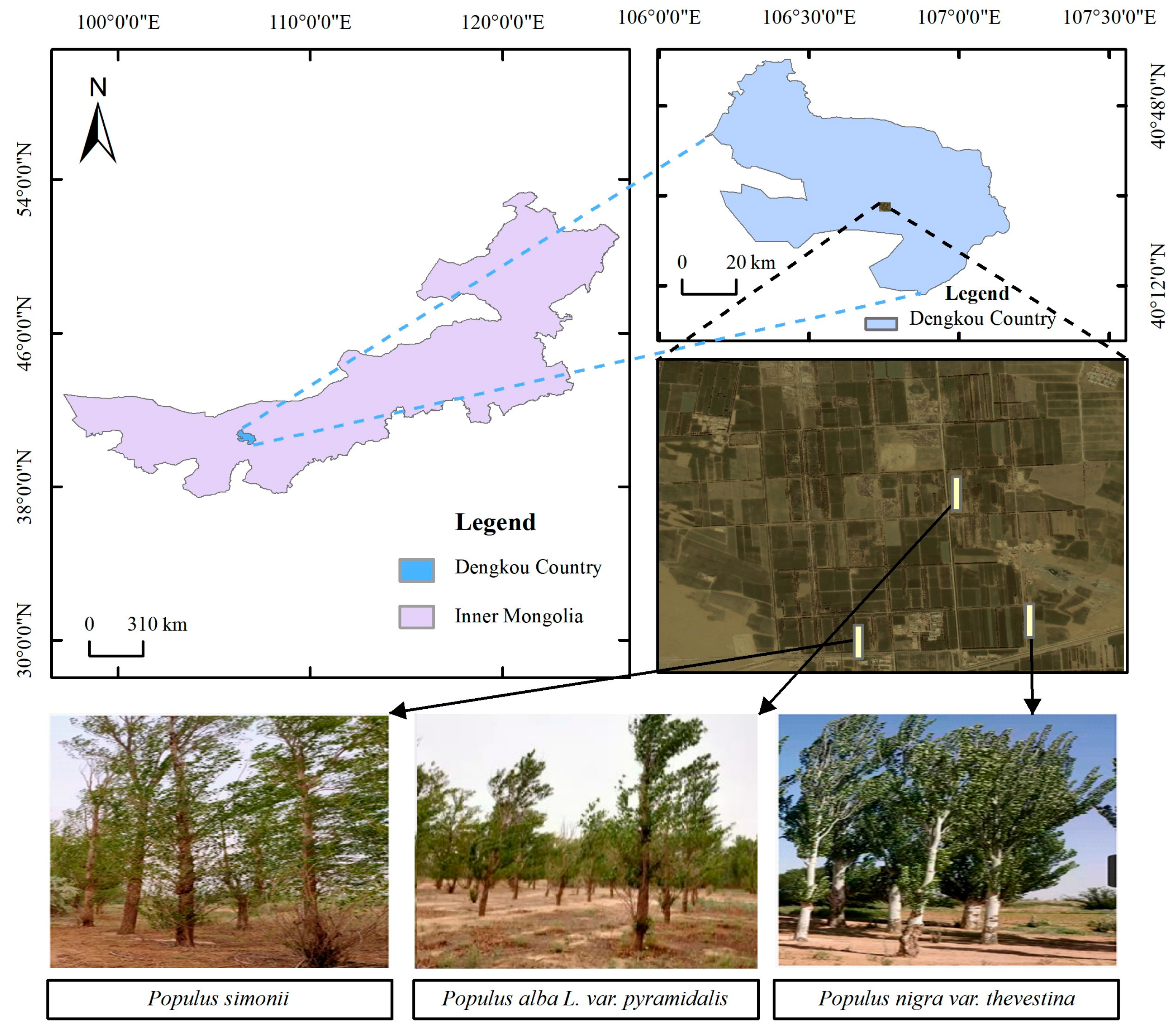
2.1. Study Area

The study plot is located in Dengkou County, Bayannaoer City, Inner Mongolia, China (40°17′–40°29′N, 106°35′–106°59′E) (Figure 1). This region features a temperate continental monsoon climate characterized by an average annual temperature of 8 °C and an average annual precipitation of 144 mm. The precipitation is mainly concentrated from June to September and the annual evaporation is 2398 mm. The prevailing wind in the area is from the northwest, with an average annual wind speed of 4.1 m/s, and the maximum instantaneous wind speed can reach 24 m/s. The predominant soil types are sandy soil and sandy loam. The tree species in the agricultural shelterbelt forests mainly consist of Populus alba var. pyramidalis, Populus simonii, and Populus nigra var. thevestina.

2.2. Data

2.2.1. Field Survey Data

This experiment selected three typical tree species as subjects, namely, Populus alba var. pyramidalis, Populus simonii, and Populus nigra var. thevestina (

Table 1. Basic information on shelterbelts.

Species	Row	Age (a)	Shelterbelt Length and Width (m)	Spacing (m)	Direction	Number
Populus alba var. pyramidalis	5	28	450 × 20	4.5 × 5	north-south	450
Populus simonii	4	35	196 × 15	4 × 5	north-south	192
Populus nigra var. thevestina	8	33	390 × 35	5 × 5	north-south	378

). From July to August 2021, three sample were randomly chosen within each shelterbelt and the trees within these quadrats were examined for various parameters. These parameters included diameter at breast height (DBH), tree height, crown diameter, and other data. A total of six Populus alba var. Pyramidalis trees, six Populus simonii trees, and three Populus nigra var. Thevestina trees were chosen from all sample plots for accuracy assessment of TLS parameter extraction and algorithm tuning. This study adopted the method for categorizing tree decline levels previously established by Wang et al. [28]. The classification involves three levels based on the proportion of dead branches (the percentage of secondary and tertiary dead branches in the tree’s main stem branches): normal growth when the proportion is ≤10%, mild decline when it’s >10% and ≤30%, and severe decline when it’s >30%. Following an evaluation of the proportions of dead branches across all trees within the three shelterbelts, the Populus alba var. pyramidalis belt contains a total of 450 individual trees, with 303 growing normally, 67 experiencing mild decline, and 80 exhibiting severe decline. In the Populus simonii belt, there are 192 individual trees, with 145 growing normally, 16 experiencing mild decline, and 31 exhibiting severe decline. Similarly, in the Populus nigra var. thevestina belt, there are 378 individual trees, with 308 growing normally, 33 experiencing mild decline, and 37 exhibiting severe decline.

2.2.2. LiDAR Data Acquisition and Processing

TLS (RIGEL VZ-400i) was utilized to collect raw point cloud data from the shelterbelts. Its scanning range encompassed 360° horizontally and 100° vertically, achieving an accuracy of 5 mm. The RiSCANPro 2.0 software, which is compatible with the TLS, was utilized for automated point cloud data stitching. For data segments that could not be automatically stitched, manual stitching was conducted using control points marked by targets. The CloudCompare v2.10.alpha software was used for point cloud denoising, ground point separation, and single tree segmentation. The statistical filtering algorithm was employed for noise removal, with a set of parameters: neighborhood point count N set at 20, and standard deviation multiplier T set at 2. The outliers not automatically removed were manually eliminated. The cloth simulation filtering method was used to eliminate ground points [29]. Considering the study area’s relatively flat terrain, the flat mode was adopted, with a ground classification threshold set at 0.2 m and a maximum iteration count of 500. The Lidar 360, employing the Triangulated Irregular Network (TIN) interpolation, was utilized for elevation normalization of point cloud data. For accurate segmentation of single trees, manual segmentation of point cloud data was performed. of Row and column position information for each tree was manually recorded. The LeWoS was used for separating branches and leaves from the segmented tree files [30], with a threshold of 0.125. The LiDAR360 was utilized to extract tree parameters, including diameter at the breast height (DBH), tree height, crown diameter, and gap fraction. The crown projection area was calculated using both the canopy contour recognition algorithm and traditional geometric methods [31]. The CanopyLazR package in Rstudio was employed to calculate leaf area index (LAI), with a voxel resolution set at 1 [9]. The TreeQSM algorithm [32] was executed in Matlab R2018a to compute the tridimensional green biomass of trees, with the PathDiam set at 0.04 m. In this study, seven single tree structural parameter variables were extracted to characterize tree growth horizontally and vertically (

Table 2. Tree structure parameters and description extracted from TLS.

Label	Index	Description
I1	Diameter at breast height	Diameter of the tree trunk at 1.3 m above ground level
I2	Tree height	Distance from the top of the stand vertically to the ground
I3	Crown diameter	Diameter of each tree crown
I4	Crown projection area	Area of the forest canopy projected vertically on the ground
I5	Tridimensional green biomass	Volume of space occupied by total plant stems and leaves
I6	Leaf area index	Ratio of the total leaf area per unit land area to the land area
I7	Gap fraction	Probability of light passing through the canopy and reaching the surface without being intercepted

).

In addition to the seven structural variable parameters, this study also extracted radiometric variables from the LiDAR data, including height, intensity, and density variable information [26]. Among these, the height variable information primarily characterizes the three-dimensional structure of the trees. The intensity variable information reflects differences in intensity for various materials, such as leaves and woody substances. The density variable depicts how the crown point cloud is distributed in space, highlighting aggregation and dispersion tendencies. The specific feature parameters are presented in the

Table 3. Radiation variable parameters extracted from TLS (H is the height of an individual point, D is the density of an individual point, and I is the intensity of an individual point).

Labels	Indices	Description
I8	Haad	Average absolute deviation of the height of the tree points: mean(abs(H − Havg))
I9	Hccr	Canopy relief ratio of tree points: (Havg − Hmin)/(Hmax − Hmin)
I10–I24	Hcuh1-Hcuh99	Cumulative height percentiles (i.e., 1, 5, …, 99) of tree points
I25	Hcv	Coefficient of variation of the height of the tree points
I26	Hkur	Kurtosis of the height of the tree points
I27	Hmad	Median absolute deviation of the height of the tree points: median(abs(H − Hp50))
I28	Hmax	Maximum height of the tree points
I29	Hmin	Minimum height of the tree points
I30	Havg	Average height of the tree points
I31	Hmed	Median height of the tree points
I32–I46	Hhei1-Hhei99	Height percentiles (i.e., 1, 5, …, 99) of tree points
I47	Hske	Skewness of the height of the tree points
I48	Hstd	Standard deviation of the height of the tree points
I49	Hvar	Variance of the height of the tree points
I50–I59	Dsp1-Dsp10	1st, 2nd… 10th slices point cloud density
I60	Iaad	Average absolute deviation of intensity of tree laser returns: mean(abs(I − Iavg))
I61	Icv	Coefficient of variation of intensity of tree laser returns
I62–I76	Icip1-Icip99	Cumulative intensity percentiles (i.e., 1, 10, …, 99) of tree laser returns
I77	Ikur	Kurtosis of intensity of tree laser returns
I78	Imad	Median absolute deviation of intensity of tree laser returns: median(abs(I − Ip50))
I79	Imax	Maximum intensity of tree laser returns
I80	Imed	Median intensity of tree laser returns
I81	Iavg	Average intensity of tree laser returns
I82	Imin	Minimum intensity of tree laser returns
I83	Iske	Skewness of intensity of tree laser returns
I84	Ivar	Variance of intensity of tree laser returns
I85	Istd	Standard deviation of intensity of tree laser returns
I86–I100	Ip1–Ip99	Intensity percentiles (i.e., 1, 5, …, 99) of tree laser returns
I101	Iipr	Inter-percentile range of intensity of tree laser returns: Ip75–Ip25

.

2.2.3. Hyperspectral Imagery Acquisition and Processing

The HI data of the shelterbelts were acquired on 13 August 2021, under clear and cloudless weather conditions. The data collection occurred from 12:00 to 13:00. An unmanned aerial vehicle operated at an altitude of 100 m, covering a flying area of 500 m by 50 m. The flight speed was 5 m per second, and the imaging was conducted in a vertical downward observation mode. The Corning^® microHSI™410 SHARK sensor (Corning Inc., Corning, NY, USA) was used for capturing imagery, spanning a spectral range from 400 to 1000 nm (interval 2 nm). The imagery was obtained via a push-broom scanning mode employing a linear array detector.

Before and during the acquisition of the hyperspectral data, white reference panels were deployed for reflectance calibration of the raw spectral data. Due to the small size of the study area, no stitching was performed. To mitigate random errors introduced by the instrument, the Savitzky–Golay smoothing algorithm was applied for data denoising [33]. The derivative order was set to 0, the smoothing points were set to 5, and the polynomial degree was set to 3. Matlab R2018a was utilized for Savitzky–Golay filtering, first-order differentiation, and second-order differentiation of the original spectral curves. The raw data of the spectral curves were extracted using ENVI 5.3, followed by reflectance calibration, geometric correction, clipping, and band calculation.

To capture subtle variations in the spectral curves of trees more effectively, this study calculated spectral derivative values (first and second order) to eliminate the influence of external factors such as temperature. To comprehensively assess the plant growth condition, this study utilized fluctuation operations to derive vegetation indices (

Table 4. The selected vegetation indices and formula (R_i represents the spectral reflectance at band i, for example, R₄₅₀ represents the spectral reflectance at 450 nm).

Indices	Formula
Normalized difference vegetation index (NDVI)	(RNIR − Rred)/(RNIR + Rr)
Simple ratio index (RVI)	RNIR/Rred
Enhanced vegetation index (EVI)	2.5(RNIR − Rred)/[RNIR + 6Rred − 7.5Rblue + 1)
Atmospherically resistant vegetation index (ARVI)	[RNIR − 2(Rred − Rblue)]/[RNIR + 2(Rred − Rblue)]
Red-edge normalized difference vegetation index (NDVI705)	(R750 − R705)/(R750 + R705)
Modified red-edge simple ratio index (mSR705)	(R750 − R445)/(R705 + R445)
Modified red edge normalized difference vegetation index (mNDVI705)	(R750 − R705)/(R750 + R705 − 2R445)
Sum green index (SGI)	$mean({\displaystyle \sum _{i=500}^{600}Ri})$
Vogelmann red-edge index 1 (VOG1)	R740/R720
Vogelmann red-edge index 2 (VOG2)	(R734 − R747)/(R715 + R726)
Vogelmann red-edge index 3 (VOG3)	(R734 − R747)/(R715 + R720)
Red-edge position index (REP)	${\lambda }_i,\max (Der(R_{\lambda }{}_{{}_i}))$
Photochemical reflectance index (PRI)	(R531 − R570)/(R531 + R570)
Structure insensitive pigment index (SIPI)	(R800 − R445)/(R800 + R680)
Red green ratio index (RG)	$mean({\displaystyle \sum _{i=650}^{850}{R}_i})/mean({\displaystyle \sum _{i=450}^{650}{R}_i})$
Plant senescence reflectance index (PSRI)	(R680 − R500)/R750
Carotenoid reflectance index 1 (CRI1)	(1/R510)− (1/R550)
Carotenoid reflectance index 2 (CRI2)	(1/R510) − (1/R700)
Anthocyanin reflectance index 1 (ARI1)	(1/R550) − (1/R700)
Anthocyanin reflectance index 2 (ARI2)	R800 [(1/R550) − (1/R700)]
Water band index (WBI)	R900/R970

), which will serve as variables for subsequent construction of the tree decline models [27].

2.3. Construction of the Identification Model of Tree Decline Degree

Given the relatively small sample size in the mild decline and severe decline categories, this study aimed to bolster the accuracy of the tree decline identification model by implementing data sampling procedures [27]. The chosen method was random oversampling, and prior to the sampling, feature selection was carried out. Correlation analysis and stepwise regression analysis were employed to select the spectral and LiDAR feature parameters of the trees. We used repeat sampling method to ensure that the model validation contains samples that were oversampled.

Using random forest (RF), artificial neural network (ANN), support vector machine (SVM), k-nearest neighbor (KNN), light gradient boosting machine (LightGBM), multilayer perceptron (MLP) classification methods to establish the degree of decline identification model [34] in order to explore the feasibility of each classification algorithm to identify the degree of tree decline. The model was constructed by using the field-measured canopy withering as the target observation, and the characteristic parameters extracted from LiDAR data and HI data as the predictors. The overall dataset was subjected to a random sampling of 10% for predictive purposes. Within the remaining 90% of the data, 20% was designated as testing data, with 80% allocated as training data. This iterative process was conducted 10 times to ensure statistical robustness. The research was conducted utilizing the Windows 10 operating system, leveraging Anaconda 3 as the integrated development environment, and utilizing Python 3.8 as the programming language. The development of the six models was executed using Keras 2.7.0 and TensorFlow 2.7.0. The neural network intelligence (NNI) platform was harnessed to optimize hyperparameters for each model. Four parameters (learning rate, regularization parameter, batch size, and hidden layer size) have been adjusted.

2.4. Accuracy Evaluation

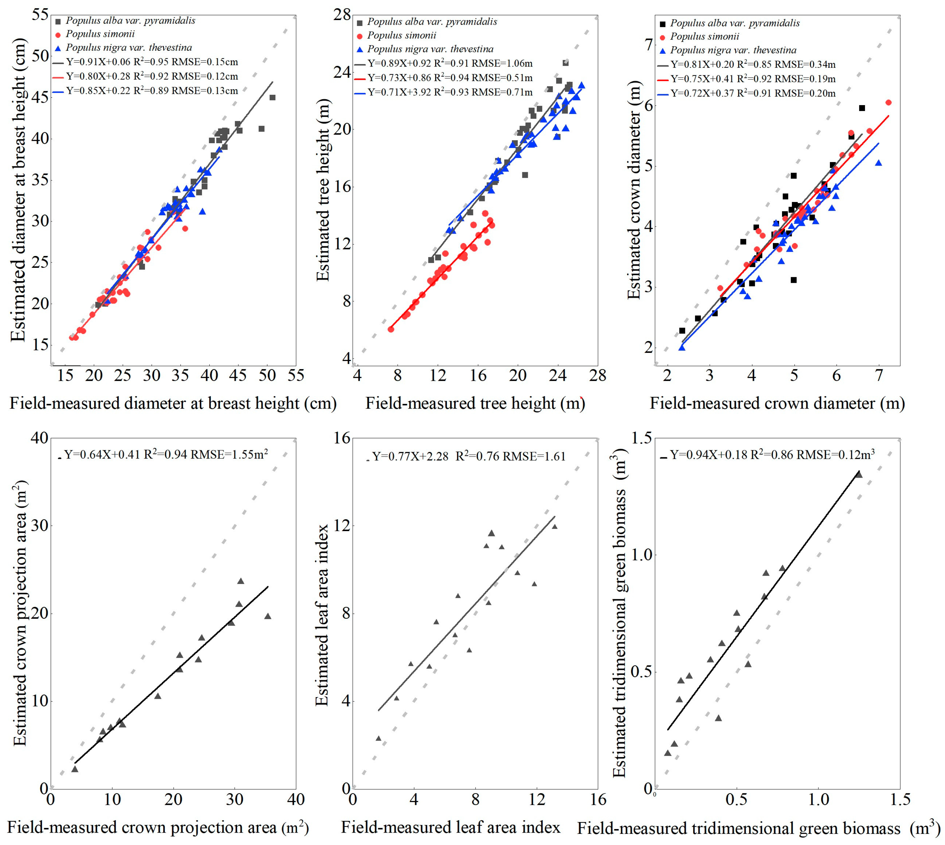
2.4.1. Accuracy Calculation of Structure Parameters Extracted by TLS

To investigate the accuracy of algorithms for extracting single tree structural parameters based on LiDAR data, a comparison was made between field-measured values of parameters and the values extracted from LiDAR data. The precision of the extracted values in comparison to the measured values was assessed through the calculation of root mean square of errors (RMSE) and coefficients of determination (R²) between LiDAR point cloud-derived values and actual measurements. The formulas for calculating RMSE and R² are as follows:

$$RMSE=\sqrt{\frac{{{\displaystyle {\sum }_1^n(y_i-y_i{}^{*})}}^2}{n}}$$

(1)

$${{\displaystyle R}}^2=1-\frac{{\displaystyle {\sum }_{i=1}^n{(y_i{}^{*}-y_i)}^2}}{{\displaystyle {\sum }_{i=1}^n{(y_i-\overline{y})}^2}}$$

(2)

where y_i and y_i* represent the field-measured values and the extracted values of the structural parameters, respectively, ȳ stands for the mean value of the field-measured structural parameters, and n denotes the total number of field-measured structural parameter values.

2.4.2. Calculation of the Accuracy of the Decline Degree Identification Model

Common accuracy evaluation metrics for classification models include overall accuracy (OA) and the Kappa coefficient (Kc). In this context, OA is defined as the percentage of correctly classified instances out of the total instances. Kc is typically calculated using a confusion matrix [35].

$$OA=\frac{{\displaystyle \sum _{i=1}^n{X}_{ii}}}{{\displaystyle \sum _{i=1}^n{\displaystyle \sum _{j=1}^n{x}_{ij}}}}$$

(3)

$$kappa=\frac{N{\displaystyle \sum _{i=1}^n{X}_{ii}}-{\displaystyle \sum _{i=1}^n(X_{i+}+X_{+i})}}{N^2-{\displaystyle \sum _{i=1}^n(X_{i+}+X_{+i})}}$$

(4)

where n represents the number of classification categories; X_ii signifies the count of pixels in the confusion matrix at the intersection of the ith row and ith column (number of correctly classified items); X_i+ and X_+i denote the total number of categories in row jth (divided into target categories) and column jth (real samples of target categories), respectively; N is the total number of samples.

3. Results

3.1. Accuracy Analysis of Extracting Forest Structure Parameters by TLS

The linear fitting results between field-measured and LiDAR-extracted values for DBH, tree height, and crown width showed good performance across three tree species (Figure 2), with R² values ranging from 0.85 to 0.95. The highest and lowest R² values were associated with DBH for Populus alba var. pyramidalis (0.95) and tree height for Populus nigra var. thevestina (0.85), respectively. The average R² values for DBH, tree height, and crown width across the three tree species were 0.92, 0.93, and 0.89, respectively. The corresponding average RMSE values were 0.13 cm, 0.76 m, and 0.24 cm.

The linear regression relationships between field-measured crown projection area, LAI, and tridimensional green biomass, and their corresponding LiDAR-extracted values, exhibit R² values ranging from 0.76 to 0.94. The highest and lowest R² values were observed for the crown projection area and LAI, respectively. Among the three structural parameters, the highest and lowest slope values were found in the tridimensional green biomass (0.94) and crown projection area (0.64), respectively.

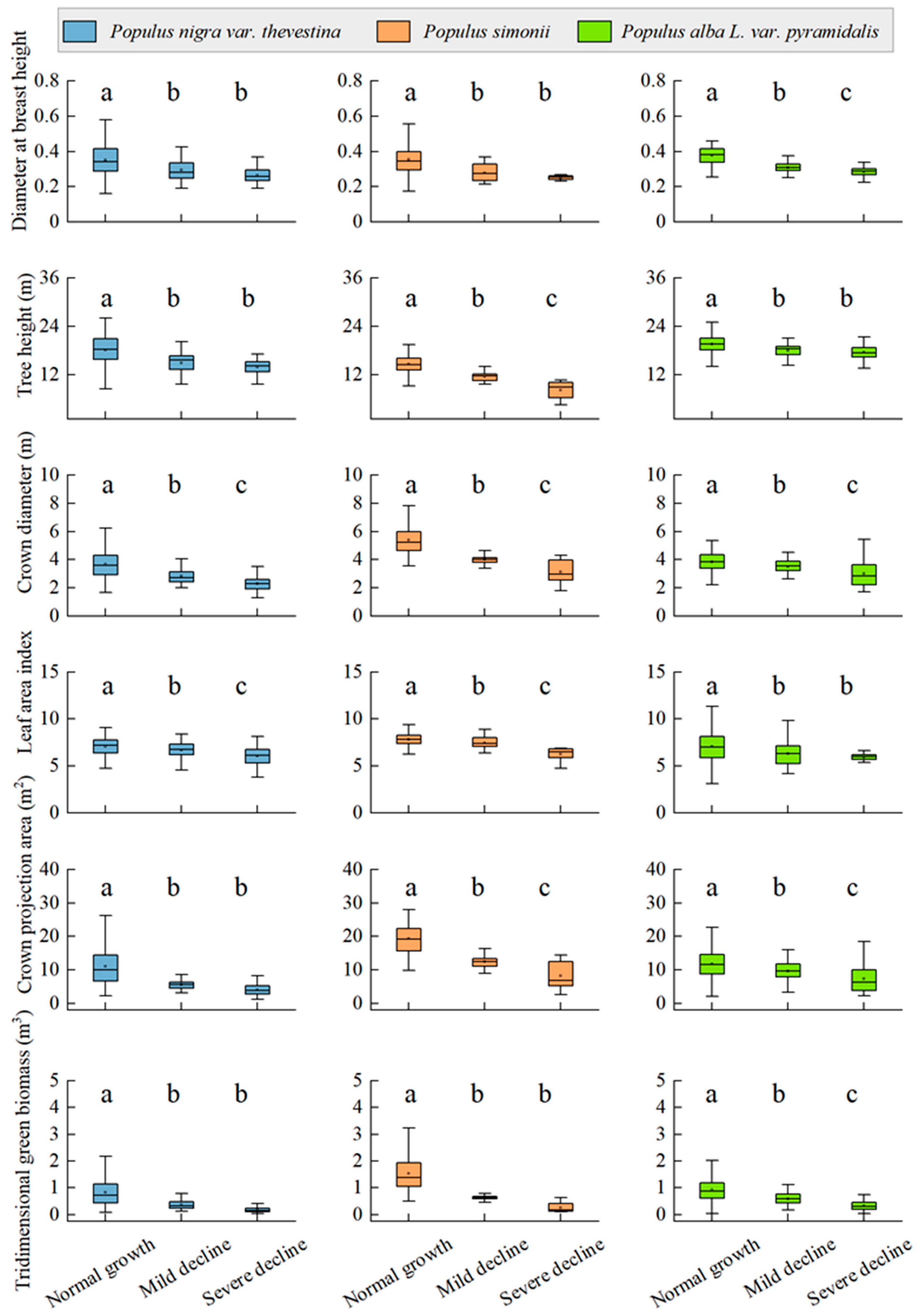
3.2. Structural Characteristics of Forest Trees with Different Degrees of Decline

The six structural parameters of trees (DBH, tree height, crown diameter, LAI, crown projection area, and tridimensional green biomass) for all three tree species gradually decreased with increasing levels of decline (Figure 3). The structural parameters of non-declined trees for all three species were significantly larger than those of trees with mild and severe decline (p < 0.05). The structural parameters of trees with mild and severe decline were reduced by 8.84–60.66% and 10.57–82.28%, respectively, compared to non-declined trees. On average, the decrease in structural parameters for declined trees compared to non-declined trees ranged from 13.65% to 63.19%. Among them, the tridimensional green biomass (63.19%) and crown projection area (44.40%) exhibited larger reductions.

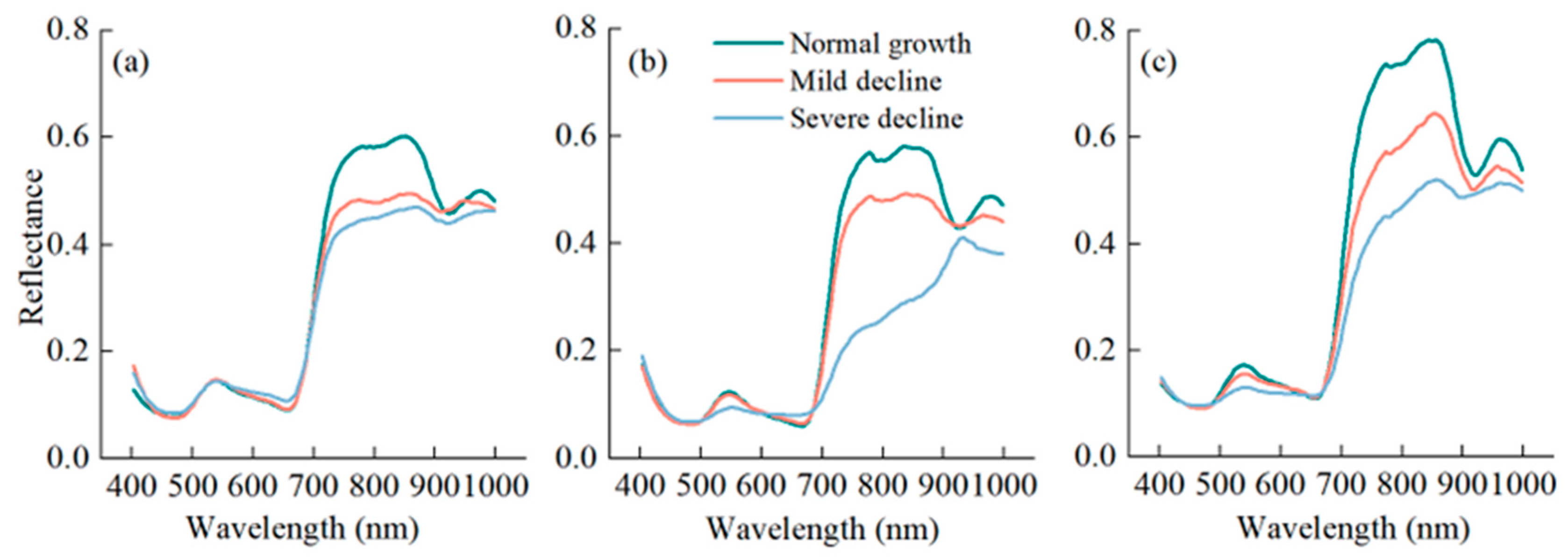
3.3. Spectral Characteristics of Forest Trees with Different Degrees of Decline

3.3.1. Raw Spectral Characteristics of Trees

In the green peak band (530–580 nm) (Figure 4), there was no significant variation observed among different degrees of decline for Populus alba var. pyramidalis. However, the spectral reflectance of Populus simonii and Populus nigra var. thevestina gradually decreased with increasing levels of decline. In the red-edge band (640–700 nm), the spectral reflectance of all three tree species increased as the degree of decline intensifies. Notably, for trees with severe decline, the spectral curve in the red-edge band exhibited a diminishing trend. Within the near-infrared band (740–950 nm), distinct changes in spectral reflectance were observed among different degrees of decline for all three tree species. The spectral reflectance of each tree species significantly decreases as the degree of decline increases, indicating a disruption in the internal canopy structure.

3.3.2. First-Order Derivative Spectral Characteristics of Trees

As the degree of tree decline intensified, within the green peak band range (530–580 nm), there was little discernible change in the first-order derivative values for Populus alba var. pyramidalis. Conversely, for Populus simonii and Populus nigra var. thevestina, the first-order derivative values of their spectra decreased as the degree of decline became more pronounced (Figure 5). In the yellow edge region (550–582 nm), all three tree species exhibited distinct absorption valleys in the first-order derivative curves of canopy spectra. These absorption valleys gradually disappeared as the degree of decline increased. Within the range of 680–740 nm, as the degree of decline intensified, the peak values in the first-order derivative curves for all three tree species gradually decreased. Simultaneously, a slight shift towards the blue end of the spectrum was observed, maintaining consistency with the changing trends of the original spectral curves. In the range of 750–990 nm, there was little noticeable variation in the characteristics of the first-order derivative curves of canopy spectra among the three tree species with different degrees of decline.

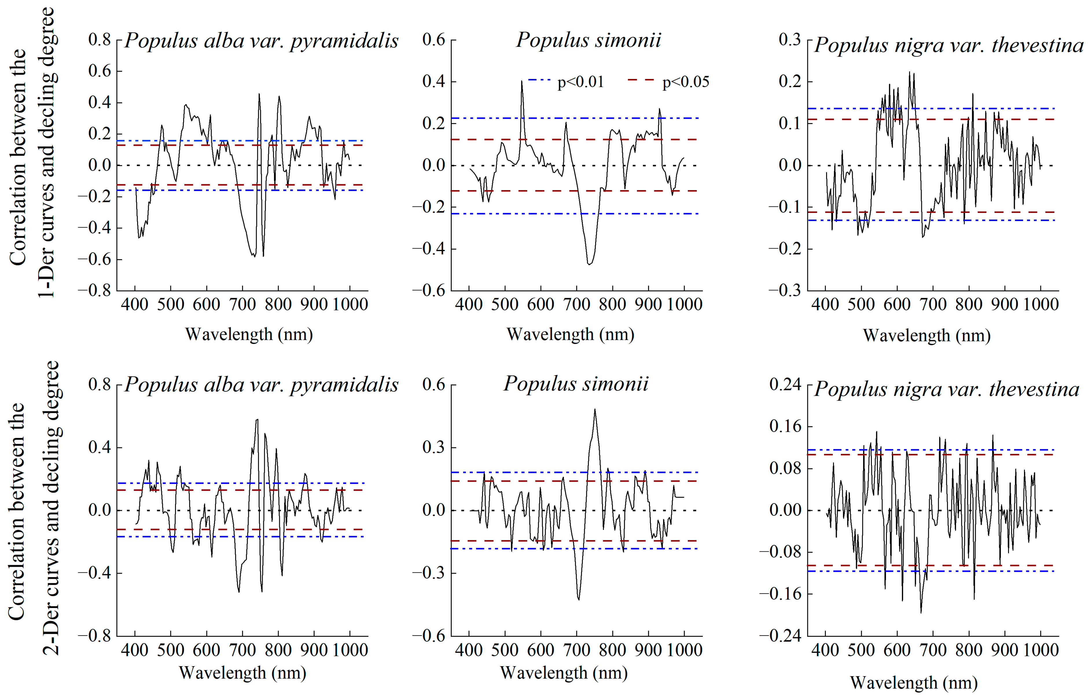
3.3.3. Correlation between the Degree of Decline and Spectral Reflectance

The correlation coefficients between the first and second order derivative values of canopy spectra (Figure 6), and the degree of decline for the three tree species ranged from −0.583 to 0.457 and from −0.522 to 0.580, respectively. For Populus alba var. pyramidalis, the spectral bands with the strongest correlation to the degree of decline were 734 nm (r = −0.583, p < 0.01) for the first-order derivative and 742 nm (r = 0.580, p < 0.01) for the second-order derivative. For Populus simonii, the spectral bands with the strongest correlation to the degree of decline were 734 nm (r = −0.475, p < 0.01) for the first-order derivative and 750 nm (r = 0.485, p < 0.01) for the second-order derivative. For Populus nigra var. thevestina, the spectral bands with the strongest correlation to the degree of decline were 634 nm (r = 0.224, p < 0.01) for the first-order derivative and 666 nm (r = −0.196, p < 0.01) for the second-order derivative.

3.4. Screening of Parameters Characterizing Forest Decline

3.4.1. Characteristic Parameters Based on TLS

Through stepwise regression analysis, feature indicators were selected (p < 0.05) (Figure 7). For Populus alba var. Pyramidalis, Populus simonii, and Populus nigra var. thevestina, the optimized laser scanning structural and radiometric variables were narrowed down to 16, 10, and 16 variables, respectively. The correlation coefficients (r) between the selected laser scanning feature parameters and the degree of decline for the three tree species ranged from −0.684 to 0.475, with an average absolute correlation coefficient of 0.381. The most highly correlated optimized variables for Populus alba var. pyramidalis, Populus simonii, and Populus nigra var. thevestina are the Hccr (I9, r = −0.684, p < 0.01), Dsp8 (I57, r = −0.544, p < 0.01), and Dsp8 (I57, r = −0.534, p < 0.01), respectively.

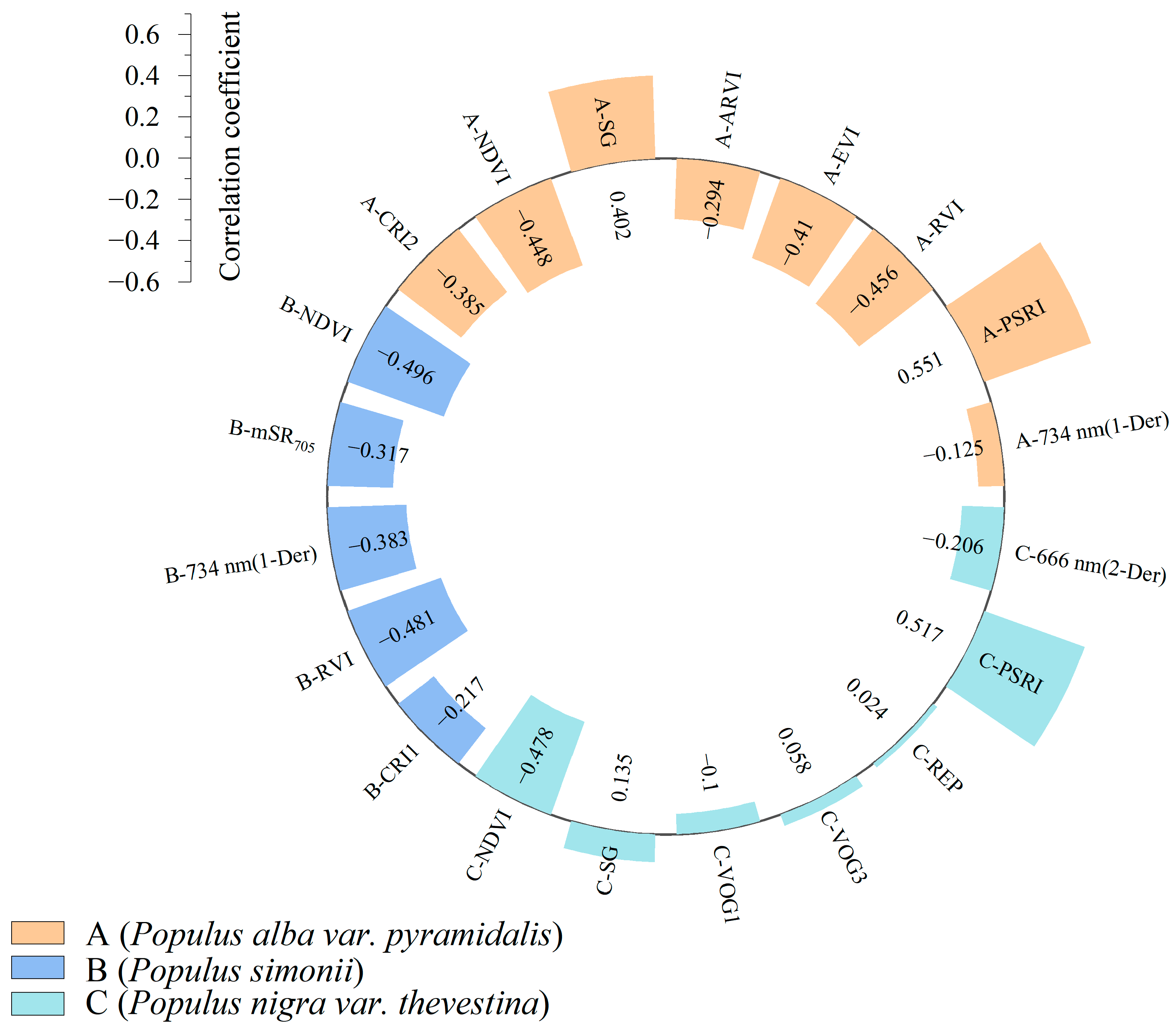
3.4.2. Characteristic Parameters Based on AHI

The results of hyperspectral index selection are presented in Figure 8. For Populus alba var. Pyramidalis, Populus simonii, and Populus nigra var. thevestina, the optimized AHI variables were narrowed down to 8, 5, and 7 variables, respectively. The correlation coefficients (r) between the selected hyperspectral feature parameters and the degree of decline for the three tree species range from −0.496 to 0.551, with an average absolute correlation coefficient of 0.324. The most highly correlated optimized variables for Populus alba var. pyramidalis, Populus simonii, and Populus nigra var. thevestina were the PSRI (r = 0.551, p < 0.01), NDVI (r = −0.496, p < 0.01), and PSRI (r = 0.517, p < 0.01), respectively.

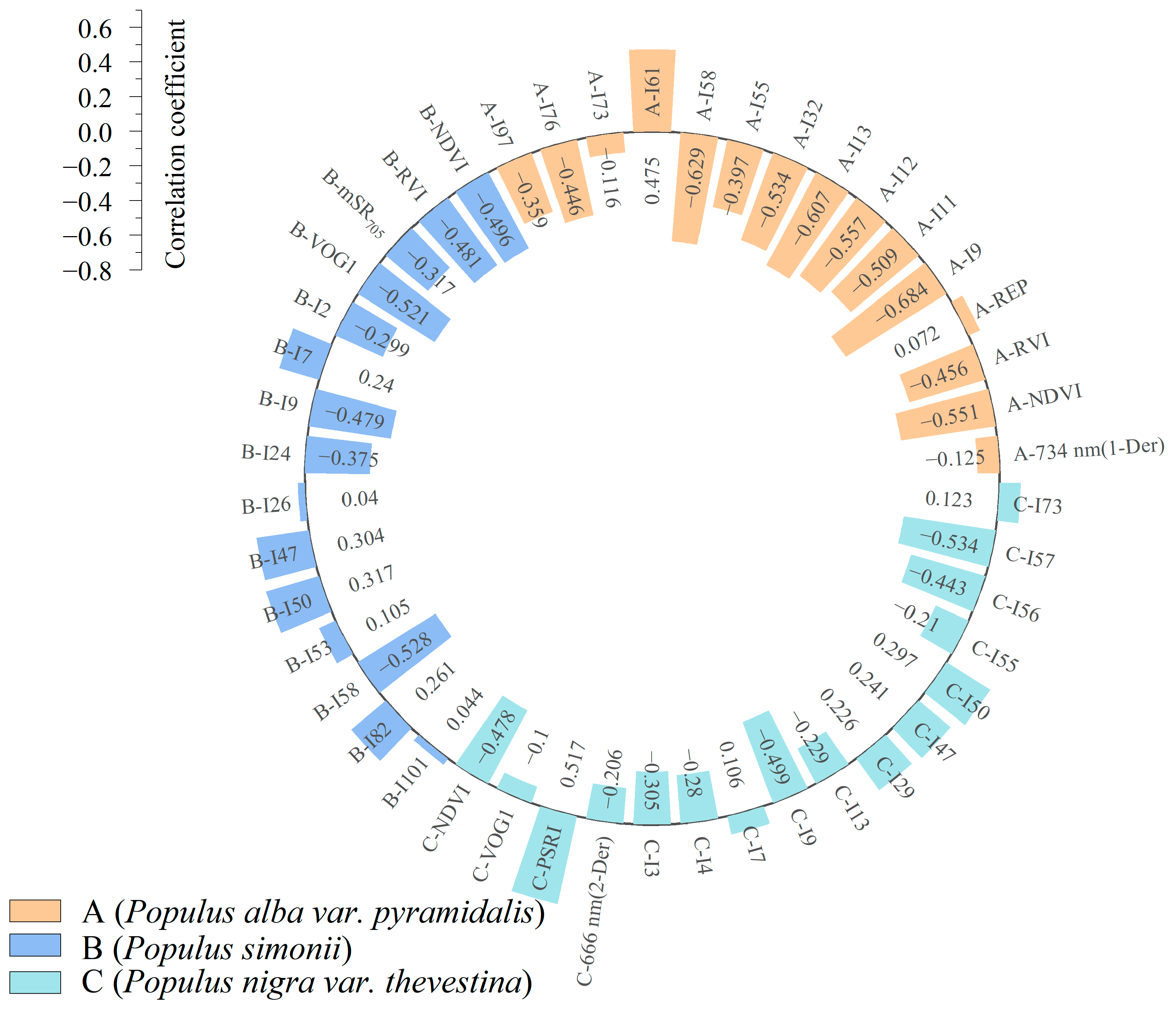
3.4.3. Characteristic Parameters Combining AHI and TLS

The results of the integrated selection of hyperspectral and LiDAR indices are presented in the Figure 9. For Populus alba var. Pyramidalis, Populus simonii, and Populus nigra var. thevestina, the optimized AHI variables were narrowed down to 15, 15, and 16 variables, respectively. The correlation coefficients between the optimized integrated feature parameters and the degree of decline for the three tree species ranged from −0.629 to 0.517. The most highly correlated integrated variables for Populus alba var. pyramidalis, Populus simonii, and Populus nigra var. thevestina were the Hccr (I9, r = −0.629, p < 0.01), Dsp9 (I58, r = −0.528, p < 0.01), and Dsp8 (I57, r = −0.534, p < 0.01), respectively. The correlation between Hccr and tree decline was more pronounced for Populus alba var. pyramidalis than for Populus nigra var. thevestina and Populus simonii.

3.5. Construction and Accuracy Evaluation of a Model for Identifying the Degree of Trees Decline

3.5.1. Models for Identifying Tree Decline Degree Based on TLS

The overall classification accuracy of the tree decline identification model based on LiDAR feature parameters ranged from 0.61 to 0.87 (

Table 5. Accuracy of forest decline model using TLS parameters (Different lowercase letters indicate significant differences between the six model mean values of different tree species (p < 0.05)).

Species	Classification Model	OA	Kc
Populus alba var. pyramidalis	RF	0.85	0.78
	ANN	0.87	0.81
	KNN	0.75	0.62
	SVM	0.83	0.79
	LightGBM	0.84	0.76
	MLP	0.84	0.76
	Mean value	0.83 a	0.75 a
Populus simonii	RF	0.73	0.60
	ANN	0.81	0.72
	KNN	0.80	0.70
	SVM	0.84	0.82
	LightGBM	0.72	0.58
	MLP	0.79	0.68
	Mean value	0.78 a	0.68 a
Populus nigra var. thevestina	RF	0.72	0.58
	ANN	0.65	0.44
	KNN	0.69	0.48
	SVM	0.61	0.40
	LightGBM	0.74	0.62
	MLP	0.72	0.58
	Mean value	0.69 b	0.52 b

), with an average value of 0.77. For Populus alba var. pyramidalis, Populus simonii, and Populus nigra var. thevestina, the average overall classification accuracies of the tree decline identification models based on LiDAR feature parameters were 0.83 (Kc = 0.75), 0.78 (Kc = 0.68), and 0.69 (Kc = 0.52), respectively. Among the models built using LiDAR feature parameters, the best-performing models for Populus alba var. pyramidalis, Populus simonii, and Populus nigra var. thevestina were ANN, SVM, and LightGBM, while the least-performing models were KNN, LightGBM, and SVM, respectively. When considering the mean values across the three tree species, the highest and lowest accuracy in discerning tree decline were achieved by the MLP model and the KNN model, respectively.

3.5.2. Models for Identifying Tree Decline Degree Based on AHI

The overall classification accuracy of the tree decline identification model based on hyperspectral feature parameters ranged from 0.50 to 0.68 (

Table 6. Accuracy of forest decline model using AHI parameters (Different lowercase letters indicate significant differences between the six model mean values of different tree species (p < 0.05)).

Species	Classification Model	OA	Kc
Populus alba var. pyramidalis	RF	0.67	0.46
	ANN	0.58	0.37
	KNN	0.65	0.44
	SVM	0.61	0.42
	LightGBM	0.68	0.52
	MLP	0.57	0.35
	Mean value	0.63 a	0.43 a
Populus simonii	RF	0.67	0.46
	ANN	0.62	0.43
	KNN	0.60	0.40
	SVM	0.65	0.44
	LightGBM	0.59	0.38
	MLP	0.50	0.25
	Mean value	0.61 a	0.39 a
Populus nigra var. thevestina	RF	0.66	0.44
	ANN	0.65	0.44
	KNN	0.56	0.38
	SVM	0.55	0.33
	LightGBM	0.61	0.41
	MLP	0.55	0.33
	Mean value	0.60 a	0.39 a

), with an average value of 0.61. For Populus alba var. pyramidalis, Populus simonii, and Populus nigra var. thevestina, the average overall classification accuracies of the tree decline identification models based on hyperspectral feature parameters were 0.63 (Kc = 0.43), 0.61 (Kc = 0.39), and 0.60 (Kc = 0.39), respectively.

Among the models built using hyperspectral feature parameters, the best-performing models for Populus alba var. pyramidalis, Populus simonii, and Populus nigra var. thevestina were LightGBM, RF, and RF, respectively, while the poorest-performing models were all MLP. When considering the mean values across the three tree species, the highest and lowest accuracy in discerning tree decline were achieved by the RF model and the MLP model, respectively.

3.5.3. Models for Identifying the Degree of Tree Decline Based on Features Combined TLS and AHI

The overall classification accuracy of the tree decline identification model based on the integrated hyperspectral and LiDAR feature parameters ranged from 0.63 to 0.92 (

Table 7. Accuracy of forest decline model combining TLS and AHI parameters (Different lowercase letters indicate significant differences between the six model mean values of different tree species (p < 0.05)).

Species	Classification Model	OA	Kc
Populus alba var. pyramidalis	RF	0.89	0.84
	ANN	0.89	0.85
	KNN	0.63	0.44
	SVM	0.88	0.82
	LightGBM	0.90	0.85
	MLP	0.79	0.69
	Mean value	0.83 a	0.75 a
Populus simonii	RF	0.92	0.88
	ANN	0.88	0.82
	KNN	0.71	0.53
	SVM	0.80	0.71
	LightGBM	0.88	0.82
	MLP	0.86	0.78
	Mean value	0.84 a	0.76 a
Populus nigra var. thevestina	RF	0.80	0.71
	ANN	0.83	0.72
	KNN	0.78	0.68
	SVM	0.64	0.45
	LightGBM	0.86	0.74
	MLP	0.72	0.68
	Mean value	0.77 a	0.66 a

), with an average value of 0.81. For Populus alba var. pyramidalis, Populus simonii, and Populus nigra var. thevestina, the average overall classification accuracies of the tree decline identification models based on the integrated hyperspectral and LiDAR feature parameters were 0.83 (Kc = 0.75), 0.84 (Kc = 0.76), and 0.77 (Kc = 0.66), respectively. Among the models built using the integrated hyperspectral and LiDAR feature parameters, the best-performing models for Populus alba var. pyramidalis, Populus simonii, and Populus nigra var. thevestina were LightGBM, RF, and LightGBM, respectively, while the poorest-performing models were KNN, KNN, and MLP, respectively. When considering the mean values across the three tree species, the highest and lowest accuracy in discerning tree decline were achieved by the LightGBM model (OA = 0.88, Kc = 0.80) and the KNN model (OA = 0.71, Kc = 0.55), respectively.

4. Discussion

4.1. The Accuracy of Parameters Extracted by TLS and the Characteristics of Structural Parameters of Different Declining Trees

This study found that using LiDAR technology to extract individual tree parameters demonstrated a linear relationship with R² values ranging from 0.76 to 0.95 when compared to ground-truth measurements (Figure 2). This indicated that TLS rapidly and accurately extracted forest tree parameters. However, there were still errors in the data acquisition and processing process of TLS, primarily stemming from one aspect: the overlapping of crowns from neighboring trees can result in incomplete segmentation of overall tree crowns, ultimately affecting the accuracy of the single tree crown and LAI extraction. The study found that the minimum R² value was shown in LAI (0.76). This could be because the voxel-based modeling for LAI computation may incorporate tree trunk and branch point cloud data, leading to discrepancies when calculating the overall forest LAI [36]. The reconstruction of three-dimensional leaf models based on point cloud data can be considered to achieve higher precision in obtaining LAI. For Populus alba var. pyramidalis, Populus simonii, and Populus nigra var. thevestina (Figure 3), all seven structural parameters decreased gradually with increasing degrees of decline. This finding aligned with previous research results [37]. The study also indicated that changes in tree crown projection area and three-dimensional green volume were more pronounced with increasing degrees of decline. Therefore, these parameters can serve as key indicators for characterizing declining trees, providing valuable insights for the construction subsequent models.

4.2. Hyperspectral Characteristics of Trees with Different Declining Degrees

The spectral reflectance of vegetation can reflect the physiological status and growth conditions of plants [38]. This study analyzed the crown spectral characteristics of Populus alba var. pyramidalis, Populus simonii, and Populus nigra var. thevestina with varying degrees of decline. The study revealed that with the increasing degrees of tree decline (Figure 4), both the original spectral reflectance and spectral derivative values in the red-edge region gradually decreased and exhibited a “blue-shift” phenomenon (Figure 5). This suggested that the degree of tree decline can be effectively reflected by the original spectral reflectance and spectral derivative values in the red-edge region [39]. The findings of this study were consistent with previous studies conducted by Wang et al. [40]. and Ma et al. [41]. This may be attributed to the manifestation of tree decline, which involves a process where leaves transition from green to yellow and eventually become dry and fall off. During this process, the internal water content and chlorophyll content of the leaves gradually decrease, and changes in pigmentation lead to distinct variations in crown reflectance spectral characteristics. The variation in leaf internal structure and water content primarily affec the near-infrared region. As a result, the near-infrared region becomes a crucial indicator band region for characterizing the degree of tree decline. This provided feasible methods and technical means for monitoring tree declining.

4.3. Characterization Parameters and Classification Model of Forest Decay Degree

Through correlation analysis and stepwise regression analysis to optimize the selected indicator factors, the results indicated that the correlation between the laser radar indicator factors and the degree of tree decline was higher than that between the hyperspectral feature parameters and the degree of tree decline (Figure 7 and Figure 8). Among them, point cloud density and canopy relief ratio of tree points (Hccr) had the highest correlation coefficients with the degree of tree decline. This was due to the fact that, for individual trees, the upper branches were sparse due to upper branch dieback, resulting in lower point cloud density. Therefore, density variables can better characterize the degree of tree decline, which was consistent with previous research results [42,43]. Additionally, this study emphasized that the Hccr can also effectively characterize the degree of tree decline. The Hccr described the relative shape of the canopy and was the most important indicator for characterizing tree decline in this study [44]. The correlation between the Hccr of Populus alba var. pyramidalis and the degree of tree decline was higher than that of Populus nigra var. thevestina and Populus simonii. This was because the dry branches of Populus simonii and Populus nigra var. thevestina were distributed evenly from the bottom to the top, whereas the dry branches of Populus alba var. pyramidalis are concentrated mainly in the upper part of the tree. Therefore, the Hccr of Populus simonii and Populus nigra var. thevestina did not exhibit a pronounced representation as compared to Populus alba var. pyramidalis. In conclusion, for selecting characterization indicators of tree decline, it is recommended to focus on utilizing TLS to obtain the Hccr and point cloud density variables. These variables can serve as reliable indicators for estimating tree decline.

Six models for identifying degrees of tree decline were established based on three data sources. Overall, the models constructed using laser radar feature variables outperformed those constructed using hyperspectral feature variables in discriminating tree decline degrees (Table 5 and Table 6). Moreover, models combining TLS and AHI integrated feature variables achieved higher classification accuracy in identifying tree decline degrees (Table 6). This conclusion was similar to the findings of Lin et al. [45] and Chi et al. [26]. The relatively poor performance of hyperspectral sensor feature parameters in characterizing tree decline degrees may stem from factors like estimating tree canopy dieback and species differences. When using HI to segment tree canopies, the influence of undergrowth vegetation growth could lead to reduced accuracy in canopy identification, thus underestimating damage below the canopy caused by tree decline. In estimating tree decline degrees using the TLS, Populus nigra var. thevestina and Populus simonii exhibited lower accuracy compared to Populus alba var. pyramidalis. This disparity might be due to the varying degrees of dead branches from the bottom to the top of Populus nigra var. thevestina and Populus simonii, resulting in less distinct vertical structural changes. When combined with AHI and TLS data, Populus nigra var. thevestina and Populus simonii complemented the spectral data of physiological changes in trees, leading to a noticeable improvement in overall accuracy compared to models based solely on TLS data. Since the structural changes in Populus alba var. pyramidalis were significantly greater than physiological changes, the integration of multiple data sources did not yield substantial accuracy improvement. The highest and lowest accuracy in discerning tree decline were achieved by the LightGBM model and the KNN mode, respectively. (Table 7). It may be because KNN was more effective in dealing with local problems, but there may be shortcomings in dealing with global issues. Models such as RF, ANN, and LightGBM adopted more complex model structures and training methods, which can better handle global problems and improve accuracy [27]. Looking at the three tree species, the model for identifying tree decline degrees established by combining AHI and TLS data, particularly the LightGBM model, exhibited the highest accuracy. Therefore, it is recommended to combine TLS and AHI data sources and utilize the LightGBM model for assessing tree decline degrees in the Ulan Buh Desert Oasis region, as it offers the best performance. A decrease in leaf area usually means a decrease in the utilization of light energy by vegetation, leading to weakened photosynthesis and a decline in vegetation growth. A decrease in biomass density usually means a decrease in vegetation growth density, a decrease in biomass accumulation capacity, and also reflects the decline of vegetation. The extracted indicators in this study were limited; future efforts could enhance model accuracy by incorporating additional variables such as leaf area and biomass density.

5. Conclusions

This study utilized terrestrial laser scanning (TLS) and airborne hyperspectral imagery (AHI) data from three typical shelterbelts to assess the structural characteristics and canopy spectral changes of declining trees. Correlation analysis and stepwise regression analysis were applied to select AHI and TLS indicator factors, which led to the development of six models for the identification of degrees of tree decline. TLS can rapidly and accurately extract forest tree parameters from shelterbelts. The seven structural parameters of the three shelterbelts gradually decreased as the degrees of decline increased. The canopy projection area and tridimensional green biomass emerged as essential structural indicators for characterizing tree decline. The original spectral reflectance and spectral differential values in the red-edge region decreased gradually as tree decline progressed, effectively reflecting the extent of tree decline. The correlation between TLS indicators and tree decline was stronger than that between hyperspectral feature parameters and tree decline. The canopy relief ratio of tree points and point cloud density variables exhibited a significant potential for characterizing tree decline. The models constructed based on TLS data outperformed those using AHI data, with the highest accuracy achieved when combining both data sources. Across the three tree species, the LightGBM model demonstrated the highest accuracy in identifying tree decline degrees. Consequently, it is recommended that when assessing forest decline in the Ulan Buh Desert Oasis region, the combination of laser radar and hyperspectral data sources, along with the application of the LightGBM model, yield the most effective results.

References

1. Cheng, G.; Zhu, M.; Zhang, X.; Guo, Y.; Yang, Y.; Yun, C.; Wu, Y.; Wang, Q.; Wang, W.; Wang, H. Northeastern China shelterbelt-farmland glomalin differences depend on geo-climates, soil depth, and microbial interaction: Carbon sequestration, nutrient retention and implication. Appl. Soil Ecol. 2023, 191, 105068. [Google Scholar] [CrossRef]
2. Li, X.; Liu, L.; Xie, J.; Wang, Z.; Li, Y. Optimizing the quantity and spatial patterns of farmland shelter forests increases cotton productivity in arid lands. Agric. Ecosyst. Environ. 2020, 292, 106832. [Google Scholar] [CrossRef]
3. Du, J.; Wang, X.; Huo, Z.; Guan, H.; Huang, G. Response of shelterbelt transpiration to shallow groundwater in arid areas. J. Hydrol. 2020, 592, 125611. [Google Scholar] [CrossRef]
4. Liu, Z.; Jia, G.; Yu, X. Variation of water uptake in degradation agroforestry shelterbelts on the North China Plain. Agric. Ecosyst. Environ. 2020, 287, 106697. [Google Scholar] [CrossRef]
5. Saunders, A.; Drew, D.M.; Brink, W. Machine learning models perform better than traditional empirical models for stomatal conductance when applied to multiple tree species across different forest biomes—ScienceDirect. Trees For. People 2021, 6, 100139. [Google Scholar] [CrossRef]
6. Gao, Y.; Skutsch, M.; Rodríguez, D.L.J.; Solórzano, J.V. Identifying Variables to Discriminate between Conserved and Degraded Forest and to Quantify the Differences in Biomass. Forests 2020, 11, 1020. [Google Scholar] [CrossRef]
7. Qu, F.; Zhang, Q.; Lu, Z.; Zhao, C.; Yang, C. Land subsidence and ground fissures in Xi’an, China 2005–2012 revealed by multi-band InSAR time-series analysis. Remote Sens. Environ. 2014, 155, 366–376. [Google Scholar] [CrossRef]
8. Prodhan, F.A.; Zhang, J.; Bai, Y.; Sharma, T.P.P.; Koju, U.A. Monitoring of Drought Condition and Risk in Bangladesh Combined Data From Satellite and Ground Meteorological Observations. IEEE Access 2020, 8, 93264–93282. [Google Scholar] [CrossRef]
9. Hosoi, F.; Omasa, K. Voxel-Based 3-D Modeling of Individual Trees for Estimating Leaf Area Density Using High-Resolution Portable Scanning Lidar. IEEE Trans. Geosci. Remote 2006, 44, 3610–3618. [Google Scholar] [CrossRef]
10. Xun, L.; Zhang, J.; Cao, D.; Yang, S.; Yao, F. A novel cotton mapping index combining Sentinel-1 SAR and Sentinel-2 multispectral imagery. ISPRS-J. Photogramm. Remote Sens. 2021, 181, 148–166. [Google Scholar] [CrossRef]
11. Korhonen, L.; Korpela, I.; Heiskanen, J.; Maltamo, M. Airborne discrete-return LIDAR data in the estimation of vertical canopy cover, angular canopy closure and leaf area index. Remote Sens. Environ. 2011, 115, 1065–1080. [Google Scholar] [CrossRef]
12. Onojeghuo, A.O.; Blackburn, G.A. Optimising the use of hyperspectral and LiDAR data for mapping reedbed habitats. Remote Sens. Environ. 2011, 115, 2025–2034. [Google Scholar] [CrossRef]
13. Monika, M.L.; Guang, Z. Retrieving Forest Inventory Variables with Terrestrial Laser Scanning (TLS) in Urban Heterogeneous Forest. Remote Sens. 2011, 4, 1–20. [Google Scholar]
14. Wilson, N.; Bradstock, R.; Bedward, M. Detecting the effects of logging and wildfire on forest fuel structure using terrestrial laser scanning (TLS). For. Ecol. Manag. 2021, 488, 119037. [Google Scholar] [CrossRef]
15. Meunier, F.; Moorthy, S.M.K.; Deurwaerder, H.P.T.D.; Kreus, R.; Verbeeck, H. Within-Site Variability of Liana Wood Anatomical Traits: A Case Study in Laussat, French Guiana. Forests 2020, 11, 523. [Google Scholar] [CrossRef]
16. Othmani, A.; Voon, L.F.C.L.Y.; Stolz, C.; Piboule, A. Single tree species classification from Terrestrial Laser Scanning data for forest inventory. Pattern Recognit. Lett. 2013, 34, 2144–2150. [Google Scholar] [CrossRef]
17. Kumazaki, R. Application of 3D tree modeling using point cloud data by terrestrial laser scanner. J. Jpn. Inst. Landsc. Archit. 2021, 84, 527–530. [Google Scholar] [CrossRef]
18. Fan, G.; Nan, L.; Dong, Y.; Su, X.; Chen, F. AdQSM: A New Method for Estimating Above-Ground Biomass from TLS Point Clouds. Remote Sens. 2020, 12, 3089. [Google Scholar] [CrossRef]
19. Valbuena, R.; Maltamo, M.; Packalen, P. Classification of multilayered forest development classes from low-density national airborne lidar datasets. Forestry. 2016, 89, 392–401. [Google Scholar] [CrossRef]
20. Hosoi, F.; Nakabayashi, K.; Omasa, K. 3-D Modeling of Tomato Canopies Using a High-Resolution Portable Scanning Lidar for Extracting Structural Information. Sensors 2011, 11, 2166–2174. [Google Scholar] [CrossRef]
21. Näsi, R.; Honkavaara, E.; Lyytikäinen-Saarenmaa, P.; Blomqvist, M.; Litkey, P.; Hakala, T.; Viljanen, N.; Kantola, T.; Tandhuapää, T.; Holopainen, M. Using UAV-Based Photogrammetry and Hyperspectral Imaging for Mapping Bark Beetle Damage at Tree-Level. Remote Sens. 2015, 7, 15467–15493. [Google Scholar] [CrossRef]
22. Yuanyong, D.; Zengyuan, L.; Yong, P. Spectral and Texture Features Combined for Forest Tree species Classification with Airborne Hyperspectral Imagery. J. Indian Soc. Remote Sens. 2015, 43, 101–107. [Google Scholar]
23. Shaokui Ge, M.X.G.L. Estimating Yellow Starthistle (Centaurea solstitialis) Leaf Area Index and Aboveground Biomass with the Use of Hyperspectral Data. Weed Sci. 2007, 55, 671–678. [Google Scholar]
24. Ren, L. Three-Dimensional Convolutional Neural Network Model for Early Detection of Pine Wilt Disease Using UAV-Based Hyperspectral Images. Remote Sens. 2021, 13, 4065. [Google Scholar]
25. Meng, R.; Dennison, P.E.; Zhao, F.; Shendryk, I.; Rickert, A.; Hanavan, R.P.; Cook, B.D.; Serbin, S.P. Mapping canopy defoliation by herbivorous insects at the individual tree level using bi-temporal airborne imaging spectroscopy and LiDAR measurements. Remote Sens. Environ. 2018, 215, 170–183. [Google Scholar] [CrossRef]
26. Chi, D.; Degerickx, J.; Yu, K.; Somers, B. Urban Tree Health Classification Across Tree Species by Combining Airborne Laser Scanning and Imaging Spectroscopy. Remote Sens. 2020, 12, 2435. [Google Scholar] [CrossRef]
27. Iordache, M.D.; Mantas, V.; Baltazar, E.; Lewyckyj, N. A Machine Learning Approach to Detecting Pine Wilt Disease Using Airborne Spectral Imagery. Remote Sens. 2020, 101, 102363. [Google Scholar] [CrossRef]
28. Wang, Y.; Wei, J.; Zhou, M.; Liu, Y.; Sun, Y.; Zhao, X.; Guo, J. Ecological of Stoichiometric Characteristics of Populus davidiana forests with Different Growth and Decline Degrees in Southern Daxing’anling. Chin. J. Soil Sci. 2021, 52, 854–864. [Google Scholar]
29. Zhang, W.; Qi, J.; Wan, P.; Wang, H.; Xie, D.; Wang, X.; Yan, G. An Easy-to-Use Airborne LiDAR Data Filtering Method Based on Cloth Simulation. Remote Sens. 2016, 8, 501. [Google Scholar] [CrossRef]
30. Wang, D.; Momo, T.S.; Casella, E. LeWoS: A universal leaf-wood classification method to facilitate the 3D modelling of large tropical trees using terrestrial LiDAR. Methods Ecol. Evol. 2020, 11, 376–389. [Google Scholar] [CrossRef]
31. Terryn, L.; Calders, K.; Bartholomeus, H.; Bartolo, R.E.; Brede, B.; D’Hont, B.; Disney, M.; Herold, M.; Lau, A.; Shenkin, A. Quantifying tropical forest structure through terrestrial and UAV laser scanning fusion in Australian rainforests. Remote Sens. Environ. 2022, 271, 112912. [Google Scholar] [CrossRef]
32. Calders, K.; Newnham, G.; Burt, A.; Murphy, S.; Raumonen, P.; Herold, M.; Culvenor, D.; Avitabile, V.; Disney, M.; Armston, J.; et al. Nondestructive estimates of above-ground biomass using terrestrial laser scanning. Methods Ecol. Evol. 2015, 6, 198–208. [Google Scholar] [CrossRef]
33. Chen, J. A simple method for reconstructing a high-quality NDVI time-series data set based on the Savitzky–Golay filter. Remote Sens. Environ. 2004, 91, 332–344. [Google Scholar] [CrossRef]
34. Sidle, G.D. Using Multi-Class Machine Learning Methods to Predict Major League Baseball Pitches; North Carolina State University ProQuest Dissertations Publishing: Raleigh, NC, USA, 2017. [Google Scholar]
35. Meng, H.; Li, C.; Zheng, X.; Gong, Y.; Liu, Y.; Pan, Y. Research on Extraction of Camellia Oleifera by Integrating Spectral, Texture and Time Sequence Remote Sensing Information. Spectrosc. Spectr. Anal. 2023, 43, 1589–1597. [Google Scholar]
36. Zheng, G.; Moskal, L.M. Computational-Geometry-Based Retrieval of Effective Leaf Area Index Using Terrestrial Laser Scanning. IEEE Trans. Geosci. Remote Sens. 2012, 50, 3958–3969. [Google Scholar] [CrossRef]
37. Sun, L.; Chang, X.; Yu, X.; Jia, G.; Chen, L.; Liu, Z.; Zhu, X. Precipitaion and soil water thresholds associated with drought-induced mortality of farmland shelter forests in a semi-arid area. Agric. Ecosyst. Environ. 2019, 284, 106595. [Google Scholar] [CrossRef]
38. Liu, C.; Guo, J.; Cui, Y.; Lü, T.; Zhang, X.; Shi, G. Effects of cadmium and salicylic acid on growth, spectral reflectance and photosynthesis of castor bean seedlings. Plant Soil 2011, 344, 131–141. [Google Scholar] [CrossRef]
39. Zhong, L.B.; Wiktorsson, B.; Ryberg, M.; Sundqvist, C. The Shibata shift; effects of in vitro conditions on the spectral blue-shift of chlorophyllide in irradiated isolated prolamellar bodies. J. Photochem. Photobiol. B Biol. 1996, 36, 263–270. [Google Scholar] [CrossRef]
40. Wang, H.; Shi, L.; Ma, Y.; Shu, Q.; Liao, H.; Du, T. Research of Damage Monitoring Models and Judgment Rules of Pinus yunnanensis with Tomicus yunnanensis. For. Res. 2018, 31, 53–60. [Google Scholar]
41. Ma, Y.; Yang, B.; Zhao, N.; Zhang, X. Classification Diagnosis on the Damage Degree of Tomicus yunnanensis to Pinus yunnanensis Based on Hyperspectral and Airborne LiDAR. J. Southwest For. Univ. 2022, 42, 80–89. [Google Scholar]
42. Degerickx, J.; Roberts, D.A.; Mcfadden, J.P.; Hermy, M.; Somers, B. Urban tree health assessment using airborne hyperspectral and LiDAR imagery. Int. J. Appl. Earth Obs. Geoinf. 2018, 73, 26–38. [Google Scholar] [CrossRef]
43. Huo, L.; Zhang, N.; Zhang, X.; Wu, Y. Tree defoliation classification based on point distribution features derived from single-scan terrestrial laser scanning data. Ecol. Indic. 2019, 103, 782–790. [Google Scholar] [CrossRef]
44. Parker, G.G.; Russ, M.E. The canopy surface and stand development: Assessing forest canopy structure and complexity with near-surface altimetry. For. Ecol. Manag. 2004, 189, 307–315. [Google Scholar] [CrossRef]
45. Lin, Q.; Huang, H.; Wang, J.; Huang, K.; Liu, Y. Detection of Pine Shoot Beetle (PSB) Stress on Pine Forests at Individual Tree Level using UAV-Based Hyperspectral Imagery and Lidar. Remote Sens. 2019, 11, 2540. [Google Scholar] [CrossRef]
Figure 1. Overview of the study area.
Remotesensing 15 04508 g001
Figure 2. Linear regression analysis of field-measured parameters and extracted values of LiDAR.
Remotesensing 15 04508 g002
Figure 3. Change characteristics of tree structure with different decline degrees (different lowercase letters indicate significant differences between the different declining degrees in the same indices (p < 0.05)).
Remotesensing 15 04508 g003
Figure 4. Original spectral curves with different degrees of decline. The (ac) represent the Populus alba var. pyramidalis, Populus simonii, and Populus nigra var. thevestina, respectively.
Remotesensing 15 04508 g004
Figure 5. First-order derivative curves for different levels of decline. The (ac) represent the Populus alba var. pyramidalis, Populus simonii, and Populus nigra var. thevestina, respectively.
Remotesensing 15 04508 g005
Figure 6. Correlation between tree declining degree and spectral derivative value.
Remotesensing 15 04508 g006
Figure 7. Screening results of LiDAR feature factors.
Remotesensing 15 04508 g007
Figure 8. Screening results of AHI feature factors.
Remotesensing 15 04508 g008
Figure 9. Screening results of TLS combined with AHI comprehensive feature factors.
Remotesensing 15 04508 g009