Abstract
With the continuous advancement of deep learning technology, researchers have made further progress in the hyperspectral image (HSI) classification domain. We propose a double-branch multi-scale residual network (DBMSRN) framework for HSI classification to improve classification accuracy and reduce the number of required training samples. The DBMSRN consists of two branches designed to extract spectral and spatial features from the HSI. Thus, to obtain more comprehensive feature information, we extracted additional local and global features at different scales by expanding the network width. Moreover, we also increased the network depth to capture deeper feature information. Based on this concept, we devise spectral multi-scale residuals and spatial multi-scale residuals within a double-branch architecture. Additionally, skip connections are employed to augment the context information of the network. We demonstrate that the proposed framework effectively enhances classification accuracy in scenarios with limited training samples through experimental analysis. The proposed framework achieves an overall accuracy of 98.67%, 98.09%, and 96.76% on the Pavia University (PU), Kennedy Space Center (KSC), and Indian Pines (IP) datasets, respectively, surpassing the classification accuracy of existing advanced frameworks under identical conditions.
1. Introduction
A hyperspectral image (HSI) is composed of numerous contiguous narrow spectral bands, which can be regarded as the superposition of hundreds of two-dimensional grayscale images. An HSI contains abundant spatial texture features and spectral information features, providing valuable information for various remote sensing applications [1]. Hyperspectral remote sensing is extensively employed in various domains, including but not limited to land use classification [2], land cover mapping [3,4], target detection [5], precision agriculture [6], the identification of building surface materials [7], and geological resource exploration [8,9,10,11].
Due to the abundance of spectral bands and rich spectral information contained in HSI data, it presents a promising opportunity for precise ground cover classification. Therefore, it has become one of the most prominent research topics in the HSI field. However, as the dimensionality of HSI data increases, accurate parameter values become difficult to obtain through estimation when the size of training samples is insufficient relative to the feature space. Traditional techniques prove inefficient when confronted with the Hughes phenomenon caused by the high-dimensional nature of spectral channels. Moreover, the presence of redundant information and the increase in computational time due to high dimensionality may have a negative effect on HSI classification [12]. However, the advent of deep learning technology has injected new energy into HSI classification and demonstrated immense potential [13,14,15].
Deep learning technology has demonstrated remarkable potential in HSI classification in recent years [16,17,18,19]. Many studies have illustrated that CNNs are extensively employed for HSI classification and exhibit exceptional classification performance [20,21,22,23,24]. Furthermore, various CNN methods based on spectral and spatial data features of HSIs have been proposed. Hu et al. [25] proposed a five-layer CNN for HSI classification, demonstrating superior performance compared to traditional methods such as the SVM. The network solely utilizes spectral information while disregarding the amalgamation of spatial features among pixels. Given the high-dimensional nature of HSIs, employing two-dimensional convolution based on each spectral band would result in excessive computation. Therefore, a spectral-band-based feature dimensionality reduction method is proposed to extract spatial features from image data. For instance, Ruiz et al. [26] proposed a data classification model that uses kernel PCA (K-PCA) and inception network architecture to generate deep spatial-spectral features, thereby enhancing the accuracy of the classification results. Although dimensionality reduction methods can obtain spatial information from classified images and reduce computational requirements, they may result in the loss of some spectral information. To fully utilize both spectral and spatial features of HSIs, classification methods based on 3DCNN space-spectrum fusion features are constantly proposed. For instance, Li et al. [27] used 3DCNN to directly extract the combined spatial and spectral features of hyperspectral cube data without requiring complicated data preprocessing methods such as discriminant analysis and principal component analysis. This approach can simultaneously extract spatial and spectral features but demands significant computational resources and high hardware requirements [28]. In contrast, Zhong et al. [29] proposed a spectral–spatial residual network (SSRN) that utilizes residual learning to enhance feature representation in both the spectral and spatial domains. Initially, 1D convolutions are employed to extract spectral features, followed by 2D convolutions to extract spatial features. However, in the process of extracting spatial features, there is a possibility of destroying the extracted spectral features. Therefore, Ma et al. [30] and Li et al. [31] proposed a dual-branch network to simultaneously extract both types of features, resulting in superior extraction of both spectral and spatial features.
In addition to constructing the network framework based on the spectral and spatial data characteristics of HSIs, researchers have also devoted significant efforts to developing feature extraction methods. In terms of increasing network depth, in theory, the deeper the model, the more powerful its ability to express non-linearities so that it can more easily fit complex feature inputs. However, in practical applications, classification accuracy tends to decrease as the network’s depth increases. In response to the issue of declining classification accuracy in CNN models, as the network depth increases due to gradient disappearance, He et al. [32] proposed a residual network in 2016. Building upon this concept, Zhong et al. [29] introduced a spectral–spatial residual network (SSRN), and Wang et al. [33] proposed a fast, dense spectral–spatial convolutional network (FDSSC) for HSI classification with even greater depth than other deep learning methods. The multi-scale strategy stands out as an effective approach to enhance the accuracy of HSI classification [34,35,36]. Pooja et al. [37] utilized a multi-scale strategy for HSI classification and obtained a favorable classification effect.
Although significant progress has been made in hyperspectral classification research through CNN methods, the majority of these advancements still heavily rely on a substantial number of training samples [38]. Moreover, due to the complex distribution of HSI features, it is extremely expensive and time-consuming for professionals to label a large number of high-quality labeled samples. The scarcity of labeled samples poses difficulties in extracting spectral–spatial features, thereby hindering the attainment of optimal classification results. Given the abundance of spatial and spectral information present in HSIs, how to effectively extract these features with limited samples to achieve high-precision classification is a major issue.
In order to address this issue and ensure enhanced classification accuracy is achieved with a limited sample size, this paper proposes a double-branch multi-scale residual network (DBMSRN) inspired by the previous literature. The designed network framework utilizes a double-branch architecture to extract spectral and spatial features separately, reducing interference between the two types of features. Both branches are based on residual networks and combined with multi-scale strategies, which can not only increase the network depth and enhance its non-linear characteristics for extracting deeper feature information, but also broaden the network width to extract more global and local feature information with different scale receptive fields when faced with limited training samples. The main contributions are summarized as follows:
- (1)
- The authors propose a DBMSRN, a double-branch architecture that realizes the independent extraction of spectral and spatial features without interfering with each other by utilizing spectral multi-scale residuals and spatial multi-scale residuals on each respective branch.
- (2)
- Due to learning more representative features from limited training samples, we design spectral multi-scale residuals and spatial multi-scale residuals in double branches, respectively. The multi-scale structure based on dilated convolution reduces computational parameters and expands the network width to extract richer multi-scale features. Additionally, the inclusion of residual structure increases the depth of the network and enhances its non-linear expression ability.
- (3)
- We conducted comparative experiments on three distinct datasets and compared the proposed method with other advanced network frameworks. The results demonstrate that our approach achieves superior classification accuracy, highlighting its universality and effectiveness in data analysis.
The rest of this paper is structured as follows: Section 2 presents a detailed introduction to our proposed DBMSRN framework and related materials, while Section 3 describes the experimental datasets and evaluates the classification performance of our method against other advanced techniques. Section 4 discusses the impact of different proportions of training samples on the framework and verifies each module’s significance in the proposed framework through ablation experiments. Finally, Section 5 summarizes this paper and outlines future directions for research.
2. Materials and Method
2.1. HSI Pixel Block Construction
In order to fully utilize the spectral and spatial information of HSI, it is imperative to incorporate both types of data for pixel cube-based classification rather than relying solely on spectral information. For instance, if a given HSI dataset contains a total of pixels but only contains labeled pixels , and the corresponding label dataset is , which contains types of land cove labeled samples where represents the number of frequency bands and represents the number of land cover categories, the HSI is segmented with target pixel as the center to obtain a new dataset composed of 3D pixel blocks for input data in training the network. This paper uses 3D pixel blocks sized at . For cross-validation, 3D pixel blocks of input data are divided into the training set , verification set , and test set . In the command, , , and are label data corresponding to , , and .
2.2. Construction of the Multi-Scale Dilated Convolution Framework
In general, CNNs utilize fixed-size convolution kernels to extract features with fixed receptive fields [36,39]. However, multi-scale convolution can extend the range of receptive fields by utilizing multiple convolution kernels of varying sizes, thereby facilitating the more effective extraction of both global and detailed features. As illustrated in Figure 1a, three distinct sizes of convolution kernels with sizes , , and are used as illustrative examples. The feature information of three different receptive fields can be acquired through convolution kernels with varying sizes, and more comprehensive features can be obtained via feature fusion compared to fixed convolution kernels. However, as the size of the convolution kernel increases, so does the number of parameters involved in the computation. To reduce parameter calculation, dilated convolution is introduced in this paper. As illustrated in Figure 1b, a small-sized convolution kernel with dilated rate and is used to replace the large-sized and convolution kernel, respectively.
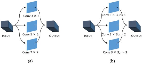
Figure 1.
(a) Multi-scale ordinary convolution. (b) Multi-scale dilated convolution.
In short, dilated convolution is the process of expanding the convolutional kernel by filling in zeros between the convolutional kernel elements. Dilated convolution can extract richer feature information by increasing the receptive field. The relationship between the expanded kernel size and the original kernel size can be determined [40]:
where is the original convolution kernel size, is the dilation rate, and is the expanded kernel size of the dilated convolution kernel. We adopt a dilation rate to indicate the degree of convolution kernel dilation. Taking a convolution kernel of size as an example, when , the dilated convolution kernel has the same size as the original convolution kernel. When , the dilated convolution kernel size is equal to the convolution kernel size .
By using multi-scale dilated convolution, on the one hand, the sparsity of dilated convolution kernels can be utilized to reduce parameter computation. On the other hand, the fusion of convolution results with different dilation rates can obtain rich multi-scale spatial information.
2.3. Construction of the Residual Block Framework
CNNs have been widely used in the field of HSI classification and have obtained fruitful research results [41,42]. Deeper models, which means better non-linear representation, can learn more complex transformations and accommodate more complex feature inputs. Nevertheless, practical applications reveal a decline in classification accuracy with an increase in network depth. This is due to the fact that, in cases of insufficient training samples, the excessively high representation ability of the CNN can result in a reduction in image information contained within each layer of feature maps during forward propagation. As convolutional layers increase in number, this can lead to gradient disappearance during backpropagation. In 2016, He et al. [32] proposed a residual network that cleverly utilizes skip connections to address this issue. As illustrated in Figure 2, the residuals block consists of a direct mapping component and a residuals component. A residual block can be mathematically expressed as:
where represents the direct mapping component of the input data, as shown in Figure 2, where the upper curve is connected by jumping, and denotes the residual component, which typically involves two or more convolution operations, as depicted in the bottom section of Figure 2 featuring a two-layer convolution operation. The architecture enables the deeper gradients to quickly propagate back to the shallower layers, effectively addressing the issue of disappearing gradients [29]. In this study, we construct spectral residuals and spatial residuals based on their respective characteristics.
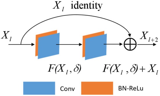
Figure 2.
The architecture of the residual model.
Notably, we incorporate BN and ReLU layers after all convolutional layers. The ReLU (Rectified Linear Unit) is a commonly used activation function in neural networks, which is one of the most popular activation functions in the field of deep research. It works by setting a threshold at 0, that is . Temporarily, the output is 0 when ; conversely, the linear function is affected when [43]. The ReLU function is computationally efficient; it can avoid vanishing gradient problems and achieve better performance in practice. Therefore, we use the ReLU as the activation function in our proposed model. Batch normalization (BN) adds standardized processing to the input data of each layer during the training process of the neural network, which can reduce the difference between samples, effectively avoid the disappearance of the gradient, and reduce the training time [44].
2.3.1. Construction of Multi-Scale Spectral Residual Blocks
In this paper, we propose a multi-scale spectral residual block that utilizes a three-layer convolution structure, as illustrated in Figure 3. We employ a two-layer convolution architecture with three independent branches between the layer and the layer . Among them, each of the three branches between the layer and the layer employs dilated convolution kernels with the size of , respectively; however, different dilation rates are utilized for each branch to extract spectral information at varying scales. The features obtained from the three branches are as follows:
where , , and represent the first branch extraction features, the second branch extraction features, and the third branch extraction features of the layer, respectively. Meanwhile, , , and denote convolution kernels with different dilation rates in the three branches, respectively. The symbol represents the convolution operation. , , and represent the bias terms in the three branches, respectively. represents the activation function. Between the layer and the layer , the three branch features extracted from the previous layer are convolved again with ordinary convolution kernels with the size of , and the three branch-extracted features are fused. In the feature fusion stage, we concatenate not only the features extracted using the three branches but also the fusion data resulting from the stepwise superposition of these features. In other words, the features extracted from the dilated convolution of the dilation rate are added pixel-by-pixel with the features extracted from the branches of the dilation rate , and the addition result is then added pixel-by-pixel with the features extracted from the branches of the dilation rate . The features obtained through pixel-wise addition comprise dilated convolution features with varying dilation rates, thereby enhancing the network’s ability to extract multi-scale features:
where , , and respectively represent the first branch extraction feature, the second branch extraction feature, and the third branch extraction feature of layer before feature fusion. , , and respectively represent the ordinary convolution kernel in the three branches, { } represents channel splicing, and represents the final extraction feature of layer . convolution kernels with a shape of are used between layer and layer . The convolution kernel in this layer can not only reduce the dimensionality, ensuring that the residual part has an equivalent number of channels as the direct mapping part, but also enhances the non-linear characteristics of the network. After performing a convolution operation, we obtain the residual part, which is then added pixel-by-pixel to the direct mapping part. Therefore, we can formulate the spectral residual structure as follows:
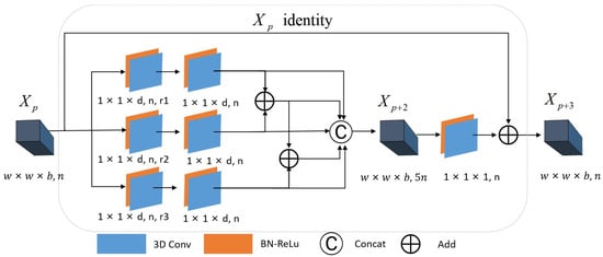
Figure 3.
The structure of multi-scale spectral residual blocks.
2.3.2. Multi-Scale Spatial Residual Block Construction
In the spatial residual block, a three-layer convolution structure is employed for spatial feature extraction, as illustrated in Figure 4. Similar to the multi-scale spectral residual block, a double-layer convolution structure with three independent branches is also used between layer and layer . Among them, the three branches between layer and layer utilize dilated convolution kernels with varying dilation rates of size to extract spatial information at multiple scales. The resulting features from these three branches are:
where , , and represent the first branch extraction features, the second branch extraction features, and the third branch extraction features of layer , respectively; , , and represent the dilated convolution kernels of the three branches with different dilation rates, respectively; represents the convolution operation; , , and represent the bias terms in the three branches, respectively; and represents the activation function. Between layer and layer , the features extracted from the three branches of the previous layer are convolved with ordinary convolution kernels of size again, and the features extracted from the three branches are fused:
where , , and respectively represent the first branch extraction features, the second branch extraction features, and the third branch extraction features of layer before feature fusion. , , and respectively represent the ordinary convolution kernel of in the three branches. { } represents channel splicing. represents the final extracted features of the layer . Between layer and layer , convolution kernels with shape are used to obtain the residual part, which is added pixel-by-pixel with the direct mapping part. Therefore, the spatial residual structure can be formulated as follows:
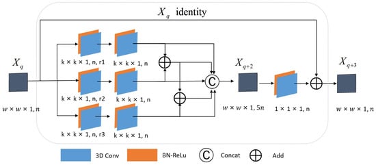
Figure 4.
The structure of multi-scale spatial residual blocks.
2.4. Proposed Framework
The proposed DBMSRN framework in this study consists of two parallel branches, namely the spectral multi-scale residual branch and the spatial multi-scale residual branch. Spectral and spatial features are extracted separately before being fused for classification. It is because the separate extraction of spectral and spatial features followed by their fusion for classification provides a more comprehensive representation of the data, captures complementary information, and allows for dimensionality reduction and flexibility in feature extraction techniques. As illustrated in Figure 5, the upper section represents the spectral multi-scale residual branch, while the lower section denotes the spatial multi-scale residual branch, which are respectively referred to as spectral and spatial branches for ease of expression. We will illustrate the designed DBMSRN in this context using a 3D pixel block as an example.
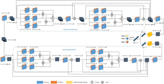
Figure 5.
The structure of the DBMSRN. The DBMSRN framework proposed in this study consists of two parallel branches. The upper branch represents the spectral multi-scale residual, while the lower branch denotes the spatial multi-scale residual.
2.4.1. Spectral Multi-Scale Residual Block Branch
The spectral branch is primarily composed of two multi-scale spectral residual blocks, two convolutional layers, and a global average pooling layer. The input of the spectral branch is a block of cubic pixels of shape . In the first convolutional layer, there are 24 channels with kernel size , after which feature cubes of shape can be obtained. The purpose of this layer is to increase the channel dimensionality of data blocks and deepen the network architecture to enhance its non-linear characteristics. Then, the two multi-scale spectral residual blocks are sequentially connected to acquire more comprehensive spectral features, while three skip connections enhance the contextual features. Each multi-scale spectral residual block includes three sets of dilated convolutional kernels with varying dilation rates with each set containing 24 channels, three sets of ordinary convolutional kernels with 24 channels, and one layer of unit convolutional kernels with 24 channels. In the multi-scale spectral residual blocks, padding is employed in each convolutional layer to maintain a consistent size of the output feature cube.
After the multi-scale spectral residual block, the feature map extracted by the first convolutional layer with the shape of , the feature map extracted by the residual part of the first multi-scale spectral residual block with the shape of , the feature map extracted by the residual part of the second multi-scale spectral residual block with the shape of , and the feature map with the shape of output from the second multi-scale spectral residual block were connected to form a final feature map output with shape . The final convolutional layer is composed of 60 1-D convolutional kernels with a shape of , which are designed to preserve discriminative spectral features. This results in feature maps of size . Subsequently, the global average pooling layer transforms the 60 spectral feature maps with the shape of into spectral feature vectors.
2.4.2. Spatial Multi-Scale Residual Block Branch
At the same time, the input data of shape is passed into the spatial branch. The first convolution layer comprises 24 channels with a 1D convolution kernel of size . Then, a feature map of shape is obtained. Subsequently, deep spatial features are acquired through two multi-scale spatial residual blocks. Each multi-scale spatial residual block consists of three sets of dilated convolutional kernels with different dilation rates and 24 channels, three sets of ordinary convolutional kernels with 24 channels, and one layer of unit convolutional kernels with 24 channels. In the multi-scale spatial residual block, padding is similarly employed consistently across all convolutional layers to maintain a constant size for the output feature cube. After the multi-scale spatial residual block, the feature maps extracted by the first convolutional layer with the shape of , the feature map extracted by the residual part of the first multi-scale spectral–spatial block with the shape of , the feature map extracted by the residual part of the second multi-scale spatial residual block with the shape of , and the feature map with the shape of that were produced by the second multi-scale spatial residual block were connected to obtain the feature map with the size of . The final convolutional layer is a unit kernel with 60 channels to preserve spatial features and generate feature maps of size . Ultimately, the extracted spatial features are transformed into feature vectors through a global average pooling layer.
2.4.3. Feature Fusion and Classification
The spectral feature vectors and spatial feature vectors are obtained through the spectral branch and spatial branch. Since the two vectors are obtained via spectral and spatial feature extraction, they belong to unrelated fields. To ensure the independence between these feature vectors, we adopt the method of channel connection for data fusion. Finally, the classification results are obtained with a fully connected layer and softmax activation function.
3. Results
3.1. Experimental Dataset
To assess the efficacy and applicability of the proposed method, we adopt three widely used HSI datasets, namely the Pavia University (PU) dataset, the Indian Pines (IP) dataset, and the Kennedy Space Center (KSC) dataset.
The PU dataset is a hyperspectral dataset acquired via the ROSIS sensor at Pavia University in northern Italy. Figure 6 shows the PU dataset’s false-color image and ground-truth classification map. It comprises 103 usable spectral bands with wavelengths ranging from 0.43 um to 0.86 um and has a geometric resolution of 1.3 m, encompassing pixels and nine distinct land cover classes.
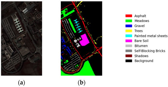
Figure 6.
(a) False-color image of Pavia University and (b) the ground truth of Pavia University.
The KSC dataset is a hyperspectral dataset acquired via the AVIRIS spectrometer at the Kennedy Space Center in Florida. Figure 7 shows the false-color image and ground-truth classification map of the KSC dataset. The dataset comprises pixels, with a total of 176 bands available within the wavelength range of 0.4 um to 2.5 um spectral bands and a spatial resolution of 18 m. It encompasses thirteen distinct ground object categories.
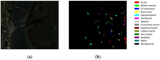
Figure 7.
(a) False-color image of the Kennedy Space Center and (b) the ground truth of the Kennedy Space Center.
The IP dataset is a hyperspectral dataset acquired in northwest Indiana using the AVIRIS sensor. Figure 8 shows the IP dataset’s false-color image and ground-truth classification map. It comprises pixels, with a total of 200 bands available within the wavelength range of 0.4 um to 2.5 um spectral bands and a spatial resolution of 20 m, encompassing 16 distinct ground object categories.
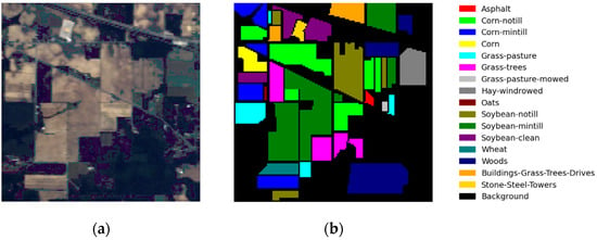
Figure 8.
(a) False-color image of Indian Pines and (b) the ground truth of Indian Pines.
Deep learning algorithms require data support, which relies on a large number of labeled training samples. The quantity of labeled training samples directly impacts the efficacy of the model, with more labeled samples leading to better results. Compared to the other two datasets, the PU dataset has a smaller variety of ground objects, but it provides sufficient labeled samples for each type with minimal discrepancies in number. In comparison to the PU dataset, the KSC dataset offers a greater variety of labeled ground objects while maintaining a relatively balanced distribution of labeled samples across different types. Conversely, the IP dataset contains the largest number of ground object categories, with some categories having significantly fewer labeled samples than others. Different distributions of labeled samples, varying spatial resolutions, and diverse imaging band ranges can impose distinct requirements on the model during the experiment. To evaluate the proposed model’s performance with limited training data, this study employs 1% of each type of labeled sample from the PU dataset for training, another 1% for validation, and reserves 98% for testing. Similarly, we use 5% of the labeled samples from both the IP and KSC datasets for each class. Table 1, Table 2 and Table 3 present the number of samples in each class for training, validation, and testing across three datasets: PU, KSC, and IN.

Table 1.
The number of samples trained, validated, and tested for each category in the PU dataset.

Table 2.
The number of samples trained, validated, and tested for each category in the KSC dataset.

Table 3.
The number of samples trained, validated, and tested for each category in the IP dataset.
3.2. Experimental Setting
All experiments in this paper are conducted on a uniform platform equipped with 16 GB memory and NVIDIA GeForce RTX 3070 GPU. All deep-learning-based classifiers are all implemented using PyTorch 1.13.0. To verify the effectiveness and universality of our proposed method, we compared it with more advanced classifiers such as the SSRN [29], the FDSSC [33], and the DBDA [31], as well as the SVM network structure with an RBF kernel [45]. To ensure consistent operating conditions across different network structures, the SSRN, FDSSC, DBDA, and the proposed method employ uniform pixel blocks of size as input, the batch size is set to 16, an Adam optimizer is used with an initial learning rate of 0.0001, the maximum number of running epochs is limited to 200, and an early stopping strategy is implemented. The SVM optimizes the penalty parameter C and the RBF kernel parameter γ using GridSearchCV in sklearn 1.1.3, since the three datasets differ in various aspects, such as ground object types, spatial resolution, and number of bands. After conducting experimental comparisons, in the PU dataset, the dilation rates for spectral multi-scale residual blocks are set to 1, 2, and 3, respectively; correspondingly, the dilation rates for spatial multi-scale residual blocks are set at 1, 2, and 4. In the KSC dataset, the dilation rates of the spectral multi-scale residual block are set to 1, 2, and 5; those of the spatial multi-scale residual block are set to 1, 2, and 3. On the other hand, for the IP dataset, dilation rates for spectral multi-scale residual blocks are set at values of 1, 2, and 4, respectively; whereas for spatial multi-scale residual blocks, they are set at values of 1, 2, and 3.
After setting the training parameters, the DBMSR network needs to train the model through the training set . The validation set is used to cross-validate the intermediate model and select the optimal network. Finally, the test set is employed to verify the generalization ability of the network. In the training process of classification problems, cross-entropy is commonly utilized as the loss function to assess the discrepancy between the predicted label and the true label , and update parameters via gradient backpropagation. This paper presents the following expressions for the predicted label and cross-entropy in the DBMSR framework:
where δ represents the model parameter of the DBMSRN to be optimized and refers to the number of classes for classification.
3.3. Experimental Results
In our experiment, we conducted five trials by randomly selecting training samples from the PU, KSC, and IP datasets to obtain an average outcome. The experimental outcomes are presented in “mean ± standard deviation” format. Table 4 displays the results for the PU dataset, with bold highlights indicating the highest accuracy achieved for a specific category. Additionally, Figure 9 illustrates the classification maps produced through different methodologies. According to Table 4, our proposed framework achieved superior classification performance with an overall accuracy (OA) of 98.67%, an average accuracy (AA) of 97.65%, and a Kappa coefficient of 0.9823, while the SVM method exhibited inferior results. When dealing with high-dimensional HIS, relying solely on spectral information for classification is insufficient and may result in salt-and-pepper noise in the resulting images. In order to standardize the operating environment, all four CNN-based frameworks uniformly utilize RELU as the activation function, so the DBDA method is less effective than the original literature, which uses MISH as the activation function. Our proposed method outperforms the SVM by approximately 10% on the PU dataset, the DBDA by approximately 3%, the SSRN by approximately 2.6%, and the FDSSN by approximately 2.5%.

Table 4.
The categorized results for the PU dataset with 1% training samples.
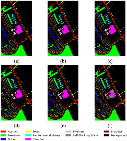
Figure 9.
Classification maps for PU dataset: (a) ground-truth map; (b) proposed method; (c) DBDA; (d) FDSSC; (e) SSRN; and (f) SVM.
The results of the KSC dataset are presented in Table 5, and Figure 10 displays the classification maps for various methods. Our method outperforms other approaches in terms of the evaluation metrics OA, AA, and Kappa on the KSC dataset. However, other methods exhibit poor classification performance due to the presence of similar classification features in the ground-truth objects of class 5, while our proposed method demonstrates some improvement in classification accuracy. Overall, the proposed method demonstrates a 6% improvement compared to the DBDA, a 5% enhancement over the FDSSC, a 1.5% advancement over the SSRN, and an impressive 9% progress beyond the SVM.

Table 5.
The categorized results for the KSC dataset with 5% training samples.
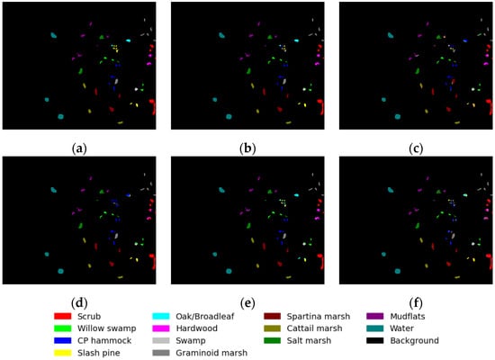
Figure 10.
Classification maps for KSC dataset: (a) ground-truth map; (b) proposed method; (c) DBDA; (d) FDSSC; (e) SSRN; and (f) SVM.
The results for the IP dataset are presented in Table 6, and Figure 11 displays the classification maps generated using various methods. Despite an imbalanced number of labeled features and only three samples for training and validation sets in class 1, class 2, and class 3, our proposed method still achieves superior classification performance. Although the proposed method exhibits an overall accuracy (OA) that is marginally higher than the FDSSC and SSRN by less than 1%, it demonstrates a significant improvement in terms of average accuracy (AA), indicating its superior balance in classifying each category. From the perspective of the classification maps, a stronger presence of salt-and-pepper noise indicates poorer classification results, while smoother maps suggest better outcomes. This qualitative comparison aligns with the quantitative evaluations of different methods.

Table 6.
The categorized results for the IP dataset with 5% training samples.
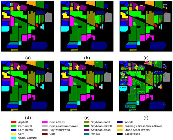
Figure 11.
Classification maps for IP dataset: (a) ground-truth map; (b) proposed method; (c) DBDA; (d) FDSSC; (e) SSRN; and (f) SVM.
4. Discussion
4.1. Classification Results of Training Sets with Varying Proportions
As previously mentioned, deep learning is a data-driven algorithm that heavily relies on a vast amount of high-quality labeled datasets. In this section, we will discuss scenarios with varying proportions of training samples. Specifically, for the PU dataset, we utilize 0.1%, 0.5%, 1%, and 1.5% of the available samples as our training set. In contrast, for the IP and KSC datasets, we use the respective sample sizes of 1%, 3%, 5%, and 7% as our training set.
As depicted in Figure 12, the overall accuracy of the five network models exhibits improvement as the number of training samples increases. The DBDA, FDSSC, SSRN, and our proposed framework all demonstrate good classification results when provided with sufficient samples. Furthermore, as the number of training samples increased, the performance gap between different models narrowed. The proposed method consistently demonstrates superior performance on the same training samples, especially in the case of low samples, both on the KSC and PU datasets with relatively balanced training samples, and on the IP dataset with large training sample gaps.

Figure 12.
The overall accuracy (OA) results of various methods under different proportions of training samples: (a) PU, (b) KSC, and (c) IP.
4.2. Ablation Experiment
An ablation experiment was carried out to demonstrate each module’s efficacy in the proposed method. The model settings varied in the ablation experiments, including Method 1, which involved removing the stepwise superposition term from the residual block; Method 2, which entailed eliminating the multi-scale dilated convolution module and replacing the three branches with a uniform small-size convolution kernel; Method 3, which transformed the double-branch structure into a network structure that first extracted spectral features and then extracted spatial features; Method 4, which eliminated all skip connection parts in the network, including the direct mapping component in the multi-scale residual blocks and the direct mapping component of the overall data fusion; Method-SPE, which retained only the multi-scale spectral residual branch; and Method-SPA, which retained only multi-scale spatial residual branches. The experimental results of different methods on three datasets of PU, KSC, and IP are illustrated in Figure 13.
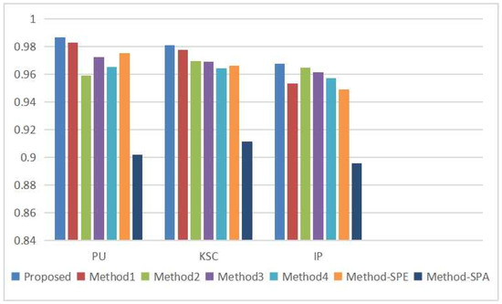
Figure 13.
Comparison of experimental ablation results of various methods in different datasets.
From Figure 13, it is evident that our proposed method outperforms other ablation experimental models in terms of classification performance on all three datasets, thereby substantiating the significance of each component of our model, including the stepwise superposition term from the residual block, the multi-scale structure based on dilated convolution, the double-branch architecture, and the direct mapping component. At the same time, it is noteworthy that the direct mapping component of the residual block plays an important role in mitigating the decline in accuracy as the depth of the network increases. The multi-scale structure can obtain more abundant feature information, which is helpful in improving classification accuracy. Moreover, the double-branch structure effectively addresses the problem of the interaction between spectral information extraction and spatial information extraction. Joint classification achieves higher accuracy than single spectral or spatial information alone. In HSI classification, spectral information yields greater accuracy in classification than spatial information.
4.3. Categorization Results with Different Combinations of Dilation Rates
To select a better combination of dilation rates, we performed some comparison experiments. Table 7, Table 8, and Table 9 show the comparison of the experimental results of the different dilation rates of spectral and spatial branches, which represent the dilation rates of the multi-scale block. To prevent the grid phenomenon, we adopt low dilation rates in this paper, and the spectral branches select a combination of , , , , , and , respectively. The spatial branch dilation rates were taken as , , and . We compared OA metrics for PU, KSC, and IP classification results for three datasets. The experimental results in Table 7 show that the best results are obtained when the dilation rate is set to 1, 2, and 3 for the spectral multiple residual blocks, respectively, and 1, 2, and 4 for the spatial multiple residual blocks, respectively, for the PU dataset. Table 8 shows the optimal effect of setting the dilation rate to 1, 2, and 5 for the spectral multi-scale residual blocks and 1, 2, and 3 for the spatial multi-scale residual blocks in the KSC dataset. On the other hand, Table 9 shows the results for the IP dataset, where the dilation rates are set to 1, 2, and 4 for the spectral multiple residual blocks and 1, 2, and 3 for the spatial multiple residual blocks. Comprehensively comparing the three datasets, the PU dataset was obtained from the ROSIS sensor with wavelengths ranging from 0.43 um to 0.86 um, while the KSC and IP datasets were obtained from the same AVIRIS sensor at wavelengths ranging from 0.4 um to 2.5 um spectral bands. The experiments show that the spatial branch dilation rates of the PU dataset are optimal at 1, 2, and 4, respectively, while the remaining two datasets are optimal at 1, 2, and 3, which may be related to the pixel spatial resolution of the HSIs. The PU dataset has a higher pixel spatial resolution than the KSC and IP datasets and is more likely to have pixels in the same class as the central pixel. In the spectral branch, the three datasets have different values, which may be related to the different correlation distances between spectral bands of different ground-based classes, but further validation with more datasets is needed.

Table 7.
The overall accuracy (OA) results for the PU dataset with different combinations of dilation rates.

Table 8.
The overall accuracy (OA) results for the KSC dataset with different combinations of dilation rates.

Table 9.
The overall accuracy (OA) results for the IP dataset with different combinations of dilation rates.
4.4. Effect of Dilated Convolution on Model Complexity
Furthermore, we discuss the effect of dilated convolutions in multi-scale residual blocks on the model’s complexity when dilated convolutional kernels with different dilation rates are replaced by ordinary convolutional kernels of corresponding sizes. As shown in Table 10, using the PU dataset as an example, we use to represent the dilation rates adopted by spectral and spatial branches, respectively, and also to represent the ordinary convolutional kernel size corresponding to the current dilation rates. We can conclude that the number of parameters increases significantly when the dilated convolutional kernels are replaced, and the larger the size of the corresponding ordinary convolutional kernel, the more parameters increase. Comparing the variation of the parameters of the spectral and spatial branches simultaneously, it can be seen that the number of parameters of the spatial branch increases much more than that of the spectral branch as the corresponding convolutional kernel size increases. Therefore, our use of dilated convolution can effectively reduce the complexity of the multi-scale model.

Table 10.
Comparison of the number of model parameters between dilated convolutions and ordinary convolutions with corresponding sizes.
5. Conclusions
We propose a double-branch multi-scale residual network framework for the more effective extraction of spectral and spatial features. At the same time, we design multi-scale residual blocks based on dilated convolution for both the spectral and spatial branches. The multi-scale dilated convolutional structure can better exploit the spatial correlation of HSIs at different resolutions and extract spectrally remote correlated features, increasing the width of the network and capturing richer feature information. The residual structure is used to effectively integrate shallow and deep features, increasing the depth of the network and improving its ability to express non-linearities. The proposed structure omits pooling layers after convolutional layers to minimize information loss in small sample training sets. This paper employs unit convolution kernels to balance channel numbers and reduce computational requirements for dimension-raising and reducing calculations. Whether it is the PU dataset with a relatively balanced number of various ground objects and high spatial resolution, the KSC dataset with a relatively balanced number of various ground objects and low spatial resolution, or the IP dataset with large differences in the number of various ground objects and low spatial resolution, experiments conducted under different proportions of training samples demonstrate that our proposed framework exhibits exceptional classification performance and shows strong robustness to different data. However, the multi-scale structure increases network parameters and subsequently prolongs training time. Therefore, future work will primarily focus on reducing time costs while conducting applicability experiments across a broader range of datasets.
Author Contributions
Conceptualization, L.F.; methodology, L.F.; software, L.F.; validation, L.F., S.P. and Y.X.; formal analysis, L.F.; investigation, L.F.; resources, X.C.; data curation, L.F.; writing—original draft preparation, L.F.; writing—review and editing, S.P.; visualization, L.F.; supervision, S.P. and Y.X.; project administration, L.F.; funding acquisition, X.C. All authors have read and agreed to the published version of the manuscript.
Funding
This research was funded by the National Natural Science Foundations of China (No. 42261075).
Conflicts of Interest
The authors declare no conflict of interest. The funders had no role in the design of the study; in the collection, analyses, or interpretation of data; in the writing of the manuscript; or in the decision to publish the results.
References
- David, L. Hyperspectral image data analysis as a high dimensional signal processing problem. IEEE Signal Process. Mag. 2002, 19, 17–28. [Google Scholar]
- Wang, H.; Li, W.; Huang, W.; Niu, J.; Nie, K. Research on land use classification of hyperspectral images based on multiscale superpixels. Math. Biosci. Eng. 2020, 17, 5099–5119. [Google Scholar] [CrossRef]
- Yan, W.Y.; Shaker, A.; El-Ashmawy, N. Urban land cover classification using airborne LiDAR data: A review. Remote Sens. Environ. 2015, 158, 295–310. [Google Scholar] [CrossRef]
- Pirasteh, S.; Mollaee, S.; Fatholahi, S.N.; Li, J. Estimation of phytoplankton chlorophyll-a concentrations in the Western Basin of Lake Erie using Sentinel-2 and Sentinel-3 data. Can. J. Remote Sens. 2020, 46, 585–602. [Google Scholar] [CrossRef]
- Eslami, M.; Mohammadzadeh, A. Developing a spectral-based strategy for urban object detection from airborne hyperspectral TIR and visible data. IEEE J. Sel. Top. Appl. Earth Obs. Remote Sens. 2015, 9, 1808–1816. [Google Scholar] [CrossRef]
- Gevaert, C.M.; Suomalainen, J.; Tang, J.; Kooistra, L. Generation of spectral–temporal response surfaces by combining multispectral satellite and hyperspectral UAV imagery for precision agriculture applications. IEEE J. Sel. Top. Appl. Earth Obs. Remote Sens. 2015, 8, 3140–3146. [Google Scholar] [CrossRef]
- Ye, C.; Cui, P.; Li, J.; Pirasteh, S. A method for recognising building materials based on hyperspectral remote sensing. Mater. Res. Innov. 2015, 19, S10-90–S10-94. [Google Scholar] [CrossRef]
- dos Anjos, C.E.; Avila, M.R.; Vasconcelos, A.G.; Pereira Neta, A.M.; Medeiros, L.C.; Evsukoff, A.G.; Surmas, R.; Landau, L. Deep learning for lithological classification of carbonate rock micro-CT images. Comput. Geosci. 2021, 25, 971–983. [Google Scholar] [CrossRef]
- Wan, Y.-q.; Fan, Y.-h.; Jin, M.-s. Application of hyperspectral remote sensing for supplementary investigation of polymetallic deposits in Huaniushan ore region, northwestern China. Sci. Rep. 2021, 11, 440. [Google Scholar] [CrossRef]
- Krupnik, D.; Khan, S. Close-range, ground-based hyperspectral imaging for mining applications at various scales: Review and case studies. Earth-Sci. Rev. 2019, 198, 102952. [Google Scholar] [CrossRef]
- Lorenz, S.; Ghamisi, P.; Kirsch, M.; Jackisch, R.; Rasti, B.; Gloaguen, R. Feature extraction for hyperspectral mineral domain mapping: A test of conventional and innovative methods. Remote Sens. Environ. 2021, 252, 112129. [Google Scholar] [CrossRef]
- Haridas, N.; Sowmya, V.; Soman, K. Comparative analysis of scattering and random features in hyperspectral image classification. Procedia Comput. Sci. 2015, 58, 307–314. [Google Scholar] [CrossRef]
- Hinton, G.E.; Osindero, S.; Teh, Y.-W. A fast learning algorithm for deep belief nets. Neural Comput. 2006, 18, 1527–1554. [Google Scholar] [CrossRef]
- Krizhevsky, A.; Sutskever, I.; Hinton, G.E. Imagenet classification with deep convolutional neural networks. Commun. ACM 2017, 60, 84–90. [Google Scholar] [CrossRef]
- Chen, Y.; Lin, Z.; Zhao, X.; Wang, G.; Gu, Y. Deep learning-based classification of hyperspectral data. IEEE J. Sel. Top. Appl. Earth Obs. Remote Sens. 2014, 7, 2094–2107. [Google Scholar] [CrossRef]
- Makantasis, K.; Karantzalos, K.; Doulamis, A.; Doulamis, N. Deep supervised learning for hyperspectral data classification through convolutional neural networks. In Proceedings of the 2015 IEEE International Geoscience and Remote Sensing Symposium (IGARSS), Milan, Italy, 26–31 July 2015; pp. 4959–4962. [Google Scholar]
- Wang, W.-Y.; Li, H.-C.; Pan, L.; Yang, G.; Du, Q. Hyperspectral image classification based on capsule network. In Proceedings of the IGARSS 2018–2018 IEEE International Geoscience and Remote Sensing Symposium, Valencia, Spain, 22–27 July 2018; pp. 3571–3574. [Google Scholar]
- Yedidia, J.S.; Freeman, W.T.; Weiss, Y. Understanding belief propagation and its generalizations. Explor. Artif. Intell. New Millenn. 2003, 8, 0018–9448. [Google Scholar]
- Hinton, G.E.; Salakhutdinov, R.R. Reducing the dimensionality of data with neural networks. Science 2006, 313, 504–507. [Google Scholar] [CrossRef]
- Zhong, Z.; Li, J.; Ma, L.; Jiang, H.; Zhao, H. Deep residual networks for hyperspectral image classification. In Proceedings of the 2017 IEEE International Geoscience and Remote Sensing Symposium (IGARSS), Fort Worth, TX, USA, 23–28 July 2017; pp. 1824–1827. [Google Scholar]
- Yu, S.; Jia, S.; Xu, C. Convolutional neural networks for hyperspectral image classification. Neurocomputing 2017, 219, 88–98. [Google Scholar] [CrossRef]
- Zhang, M.; Li, W.; Du, Q. Diverse region-based CNN for hyperspectral image classification. IEEE Trans. Image Process. 2018, 27, 2623–2634. [Google Scholar] [CrossRef]
- Yu, C.; Han, R.; Song, M.; Liu, C.; Chang, C.-I. Feedback attention-based dense CNN for hyperspectral image classification. IEEE Trans. Geosci. Remote Sens. 2021, 60, 1–16. [Google Scholar] [CrossRef]
- He, X.; Chen, Y. Transferring CNN ensemble for hyperspectral image classification. IEEE Geosci. Remote Sens. Lett. 2020, 18, 876–880. [Google Scholar] [CrossRef]
- Hu, W.; Huang, Y.; Wei, L.; Zhang, F.; Li, H. Deep convolutional neural networks for hyperspectral image classification. J. Sens. 2015, 2015, 258619. [Google Scholar] [CrossRef]
- Ruiz, D.; Bacca, B.; Caicedo, E. Hyperspectral Images Classification based on Inception Network and Kernel PCA. IEEE Lat. Am. Trans. 2019, 17, 1995–2004. [Google Scholar] [CrossRef]
- Li, Y.; Zhang, H.; Shen, Q. Spectral–spatial classification of hyperspectral imagery with 3D convolutional neural network. Remote Sens. 2017, 9, 67. [Google Scholar] [CrossRef]
- Chen, Y.; Jiang, H.; Li, C.; Jia, X.; Ghamisi, P. Deep feature extraction and classification of hyperspectral images based on convolutional neural networks. IEEE Trans. Geosci. Remote Sens. 2016, 54, 6232–6251. [Google Scholar] [CrossRef]
- Zhong, Z.; Li, J.; Luo, Z.; Chapman, M. Spectral–spatial residual network for hyperspectral image classification: A 3-D deep learning framework. IEEE Trans. Geosci. Remote Sens. 2017, 56, 847–858. [Google Scholar] [CrossRef]
- Ma, W.; Yang, Q.; Wu, Y.; Zhao, W.; Zhang, X. Double-branch multi-attention mechanism network for hyperspectral image classification. Remote Sens. 2019, 11, 1307. [Google Scholar] [CrossRef]
- Li, R.; Zheng, S.; Duan, C.; Yang, Y.; Wang, X. Classification of hyperspectral image based on double-branch dual-attention mechanism network. Remote Sens. 2020, 12, 582. [Google Scholar] [CrossRef]
- He, K.; Zhang, X.; Ren, S.; Sun, J. Deep residual learning for image recognition. In Proceedings of the IEEE Conference on Computer Vision and Pattern Recognition, Las Vegas, NV, USA, 27–30 June 2016; pp. 770–778. [Google Scholar]
- Wang, W.; Dou, S.; Jiang, Z.; Sun, L. A fast dense spectral–spatial convolution network framework for hyperspectral images classification. Remote Sens. 2018, 10, 1068. [Google Scholar] [CrossRef]
- Duan, P.; Kang, X.; Li, S.; Ghamisi, P. Noise-robust hyperspectral image classification via multi-scale total variation. IEEE J. Sel. Top. Appl. Earth Obs. Remote Sens. 2019, 12, 1948–1962. [Google Scholar] [CrossRef]
- Lu, Z.; Xu, B.; Sun, L.; Zhan, T.; Tang, S. 3-D channel and spatial attention based multiscale spatial–spectral residual network for hyperspectral image classification. IEEE J. Sel. Top. Appl. Earth Obs. Remote Sens. 2020, 13, 4311–4324. [Google Scholar] [CrossRef]
- Wu, S.; Zhang, J.; Zhong, C. Multiscale spectral-spatial unified networks for hyperspectral image classification. In Proceedings of the IGARSS 2019-2019 IEEE International Geoscience and Remote Sensing Symposium, Yokohama, Japan, 28 July 2019–2 August 2019; pp. 2706–2709. [Google Scholar]
- Pooja, K.; Nidamanuri, R.R.; Mishra, D. Multi-scale dilated residual convolutional neural network for hyperspectral image classification. In Proceedings of the 2019 10th Workshop on Hyperspectral Imaging and Signal Processing: Evolution in Remote Sensing (WHISPERS), Amsterdam, The Netherlands, 24–26 September 2019; pp. 1–5. [Google Scholar]
- Cao, F.; Guo, W. Deep hybrid dilated residual networks for hyperspectral image classification. Neurocomputing 2020, 384, 170–181. [Google Scholar] [CrossRef]
- Ali, S.; Pirasteh, S. Geological application of Landsat ETM for mapping structural geology and interpretation: Aided by remote sensing and GIS. Int. J. Remote Sens. 2004, 25, 4715–4727. [Google Scholar] [CrossRef]
- Lu, W.; Song, Z.; Chu, J. A novel 3D medical image super-resolution method based on densely connected network. Biomed. Signal Process. Control 2020, 62, 102120. [Google Scholar] [CrossRef]
- Huang, L.; Chen, Y. Dual-path siamese CNN for hyperspectral image classification with limited training samples. IEEE Geosci. Remote Sens. Lett. 2020, 18, 518–522. [Google Scholar] [CrossRef]
- Yu, C.; Han, R.; Song, M.; Liu, C.; Chang, C.-I. A simplified 2D-3D CNN architecture for hyperspectral image classification based on spatial–spectral fusion. IEEE J. Sel. Top. Appl. Earth Obs. Remote Sens. 2020, 13, 2485–2501. [Google Scholar] [CrossRef]
- Agarap, A.F. Deep learning using rectified linear units (relu). arXiv 2018, arXiv:1803.08375. [Google Scholar]
- Ioffe, S.; Szegedy, C. Batch normalization: Accelerating deep network training by reducing internal covariate shift. In Proceedings of the International Conference on Machine Learning, Lile, France, 6–11 July 2015; pp. 448–456. [Google Scholar]
- Melgani, F.; Bruzzone, L. Classification of hyperspectral remote sensing images with support vector machines. IEEE Trans. Geosci. Remote Sens. 2004, 42, 1778–1790. [Google Scholar] [CrossRef]
Disclaimer/Publisher’s Note: The statements, opinions and data contained in all publications are solely those of the individual author(s) and contributor(s) and not of MDPI and/or the editor(s). MDPI and/or the editor(s) disclaim responsibility for any injury to people or property resulting from any ideas, methods, instructions or products referred to in the content. |
© 2023 by the authors. Licensee MDPI, Basel, Switzerland. This article is an open access article distributed under the terms and conditions of the Creative Commons Attribution (CC BY) license (https://creativecommons.org/licenses/by/4.0/).