Leaf Area Index Inversion of Spartina alterniflora Using UAV Hyperspectral Data Based on Multiple Optimized Machine Learning Algorithms

Abstract

The leaf area index (LAI) is an essential biophysical parameter for describing the vegetation canopy structure and predicting its growth and productivity. Using unmanned aerial vehicle (UAV) hyperspectral imagery to accurately estimate the LAI is of great significance for Spartina alterniflora (S. alterniflora) growth status monitoring. In this study, UAV hyperspectral imagery and the LAI of S. alterniflora during the flourishing growth period were acquired. The hyperspectral data were preprocessed with Savitzky–Golay (SG) smoothing, and the first derivative (FD) and the second derivative (SD) spectral transformations of the data were then carried out. Then, using the band combination index (BCI) method, the characteristic bands related to the LAI were extracted from the hyperspectral image data obtained with the UAV, and spectral indices (SIs) were constructed through the characteristic bands. Finally, three machine learning (ML) regression methods—optimized support vector regression (OSVR), optimized random forest regression (ORFR), and optimized extreme gradient boosting regression (OXGBoostR)—were used to establish LAI estimation models. The results showed the following: (1) the three ML methods accurately predicted the LAI, and the optimal model was provided by the ORFR method, with an R² of 0.85, an RMSE of 0.19, and an RPD of 4.33; (2) the combination of FD SIs improved the model accuracy, with the R² value improving by 41.7%; (3) the band combinations screened using the BCI method were mainly concentrated in the red and near-infrared bands; (4) the higher LAI was distributed on the seaward side of the study area, while the lower LAI was located at the junction between the S. alterniflora and the tidal flat. This study serves as both theoretical and technological support for research on the LAI of S. alterniflora and as a solid foundation for the use of UAV remote sensing technologies in the supervisory control of S. alterniflora.

1. Introduction

Spartina alterniflora (S. alterniflora) is a perennial herbaceous plant native to the intertidal regions of the Atlantic coast and the Gulf Coasts of North America [1,2,3]. The various inherent biological traits of S. alterniflora, such as rapid growth, strong salt resistance, and excellent reproductive capacity through both asexual reproduction and sexual reproduction, make it suitable vegetation for the acceleration of natural land formation and the protection of the shoreline from erosion [4]. S. alterniflora was intentionally introduced to China in 1979 to buffer against tides and accelerate coastal wetland accretion [5]. Since then, it has led to numerous serious negative impacts on the natural environment and ecosystem, such as a decrease in native plant diversity, bird habitat loss, and invertebrate organism death [6,7]. In 2003, S. alterniflora was categorized as one of the first of 16 alien invasive species by the State Environmental Protection Administration of China and the Chinese Academy of Sciences [8]. Therefore, the systematic monitoring of the spatial pattern of S. alterniflora in the affected areas is of great significance to the management of invasive species.

As an essential biophysical variable with which to characterize the vegetation canopy [9], the leaf area index (LAI) usually refers to the ratio of a plant’s total green leaf area to the per-unit horizontal ground surface area [10,11]. This crucial factor influences the processes of photosynthesis, respiration, and transpiration and is closely correlated with the growth stage of the plant [12,13,14]. Thus, the precise and nondestructive monitoring of the LAI during the critical growth phase of S. alterniflora can provide information on a plant’s canopy structure, aboveground biomass, and growth in response to the ambient environment; thus, its final yield can be evaluated [15,16,17]. Traditional LAI acquisition mainly depends on manual measurement, which is time-consuming and limits the scope because of the sampling environment and data collection costs. Additionally, it cannot meet the needs for the accurate estimation of the LAI over large areas because of the vegetation heterogeneity [14,18].

Remote sensing technology can realize the large-scale and nondestructive monitoring of the physiological and biochemical parameters of vegetation, and it has developed into a crucial approach for monitoring information related to the growth of vegetation. At present, numerous studies have adopted remote sensing technology to research the physiological and biochemical parameters of vegetation [19,20]. A large number of studies on LAI monitoring have been conducted with the aid of remote sensing tools, such as handheld spectrometers [21], UAV [22], and satellites [23]. A handheld spectrometer provides the benefits of high precision and nondestructive analysis, but because of terrain accessibility, it is challenging to implement large-scale monitoring. Moreover, some researchers have employed satellite images in the estimation of LAIs; however, because of the limited resolution of satellite images compared with that of UAV remote sensing, LAI inversion has mainly been conducted on a large scale. UAVs have nondestructive and high-resolution image features for LAI monitoring, making them more suitable for the accurate monitoring of fine-scale areas. The previous research has mainly studied the LAIs of winter wheat, cotton, grassland, and others using UAV hyperspectral imagery [24], while few investigations have conducted LAI monitoring of intertidal plants or invasive species.

The flexibility and real-time nature of UAV hyperspectral images captured at the fine scale reduce the time costs of data acquisition and save financial resources [25]. With the development and popularization of UAV and hyperspectral sensors, it is possible to widely conduct low-cost nondestructive observation of vegetation parameters [26]. UAV hyperspectral images offer rich narrow-band information and more comprehensive spectral information related to LAIs, but they also introduce the problem of data redundancy [22,27,28]. Spectral indices (SIs) are robust indicators of vegetation conditions that allow for the amplification of the spectral differences among soils, vegetation, etc. [29]. Extracting canopy SIs from UAV hyperspectral images can effectively reduce data multicollinearity. The majority of the previous studies, however, acquired SIs using prior knowledge or literature research [12], and the sensitivity of the SIs with the inversion parameter was rather modest. To increase the modeling accuracy of the inversion parameters, the development of new SI prediction inversion parameters using band selection methods, like the successive projections algorithm (SPA) and the band combination index (BCI), has proved to be successful [30]. The BCI algorithm has the advantage of being able to reduce data redundancy while retaining sensitive parametric information. Liu et al. estimated the CGI of desert steppe grassland vegetation using SIs on the basis of the BCI method and the SPA. The results indicated that the BCI method was reliable, and the R² of the CGI model reached 0.78 [31]. The band selection methods and the spectral transformations have been proven to successfully minimize image noise in hyperspectral data. The sensitivity of the LAI can be improved by spectral transformation, and a certain degree of improvement in terms of precision was made to the estimation model built using hyperspectral bands [32]. Yang et al. used the first derivative (FD) and the second derivative (SD) spectral transformations and predicted UAV hyperspectral images to monitor the LAI and green leaf chlorophyll density of rice in an experimental field. By constructing three new dual-band SIs through several band selection methods using UAV hyperspectral data, Kong et al. increased the precision of the LAI estimation model [30]. As a characteristic band screen method, the BCI algorithm comprehensively utilizes the multidimensional information of hyperspectral data to obtain vegetation growth status, boosting the accuracy of the model [33]. A model based on the BCI method was adopted by Hansen et al. to screen optimal SIs with plant chlorophyll and other functional traits and to increase the estimation precision [34]. Mountrakis et al. performed FD spectral transformation of the red edge position and screened the best SIs of all possible two-band combination indices to estimate biomass through the BCI method in order to improve the model’s accuracy [35]. The spectral transformation and BCI methods have shown excellent performance in parameter inversion.

Due to their strong learning ability, machine learning (ML) algorithms have increasingly been combined with SIs to estimate LAIs, and they can find the best estimation model in complex nonlinear relationships [36]. By combining the vegetation indices of UAV hyperspectral data with various ML methods, a high-precision LAI model was obtained by Ma et al. [37]. However, some ML methods, such as artificial neural networks (ANNs), require large amounts of data for training and are also impacted by sample complexity and network structure, which increase the risk of overfitting and decrease the ability to generalize [38]. Linear models like partial least squares regression (PLSR) may fail to capture complex data patterns when dealing with nonlinear data [39]. Compared with the above ML models, the flexibility and adaptability of support vector regression (SVR), random forest regression (RFR), and extreme gradient boosting regression (XGBoostR) in dealing with various types of complex data relationships, noise, and nonlinear features mean that they can help one effectively overcome the negative impact of model estimation [40,41]. In addition, these three algorithms perform well when dealing with small-scale datasets; they are not prone to overfitting and have strong generalization abilities that have been adopted by many researchers to predict LAIs. Han et al. combined the RFR and SVR models with each vegetation index constructed from the UAV hyperspectral band to predict LAIs, demonstrating high modeling accuracy [40]. Zhao et al. also proved that the XGBoostR model had high accuracy in predicting the LAI of mangroves [41]. Although the RFR, SVR, and XGBoostR approaches have many potential applications in LAI estimates, there is currently a lack of studies on ML algorithms combined with UAV hyperspectral images that invert the LAI of S. alterniflora.

The S. alterniflora invasion is a serious threat to the ecological environment, and monitoring its LAI is helpful in understanding how it grows. Hyperspectral data can be dimensionally reduced using the combination of spectral transformation and the BCI approach to construct SIs; ML methods are crucial for LAI prediction. Thus, we adopted the FD and SD spectral transformation to process the original spectral data of Savitzky–Golay (SG) smoothing and then screened the characteristic bands through the BCI method to build new three-band SIs as input variables. Optimized support vector machine regression (OSVR), optimized random forest regression (ORFR), and optimized extreme gradient boosting regression (OXGBoostR) were employed to predict the LAI. The purposes of this paper are as follows: (1) to investigate the effect of spectral transformation on the estimation model; (2) to explore the distribution range of characteristic bands screened using the BCI method; and (3) to search for the optimal estimation model and to invert the LAI of S. alterniflora in the study area. With the optimal LAI estimation model, we can obtain the spatial distribution pattern of the LAI. As an important parameter for monitoring plant physiological processes and structural characteristics, the LAI is conducive to understanding the growth status and possible change trend of S. alterniflora, and it provides timely ecological information which wetland managers can use to formulate more reasonable control strategies [42].

2. Materials and Methods

2.1. Study Area

This study was conducted on the S. alterniflora wetlands in the coastal region located in the eastern area of Huanghua, China (117°38′21″–117°38′33″E, 38°29′10″–38°29′14″N) (Figure 1). The region has a warm temperate and semi-temperate continental monsoon climate, with an average annual precipitation of 627 mm and an average annual temperature of 12.1 °C; it is characterized as a siltation-type mudflat with a semi-diurnal tide and salinized meadow marsh soil. S. alterniflora is the dominant species, and a small number of Suaeda salsa and phragmites communis are distributed in the study area.

2.2. Datasets

2.2.1. S. alterniflora LAI

The LAI of S. alterniflora was measured during the flourishing period of 15 August 2022, using an AccuPAR LP-80 ceptometer, with a minimum of 30 meters between each LAI measurement point and the next point. A handheld high-precision GPS sampling device was used to locate and record the coordinates of the central position of each observation point with a positioning accuracy of <5 cm. To minimize illumination variations, all the operations were performed in direct sunlight between 10:00 and 14:00. The LAI measurements were taken in a circular pattern from the central location at 45-degree intervals for a total of three readings per site [43]. These three measurements were finally averaged to obtain the final LAI measurement at that specific point. With the aim of ensuring the consistency of the imagery and sampling points, 27 samples were obtained in total.

2.2.2. UAV Hyperspectral Imagery and Spectral Reflectance Process

The UAV platform consisted of a DJI M300 Pro UAV and a Cubert ULTRIS X20 Plus hyperspectral imager. The hyperspectral imagery captured with the X20 Plus consisted of 164 bands with wavelengths ranging from 350 nm to 1002 nm. The spectral resolution of the hyperspectral data was 10 nm, while the sampling interval was 4 nm. The image was captured on 15 August 2022, during the flourishing period of S. alterniflora, which is a crucial stage for its growth and development.

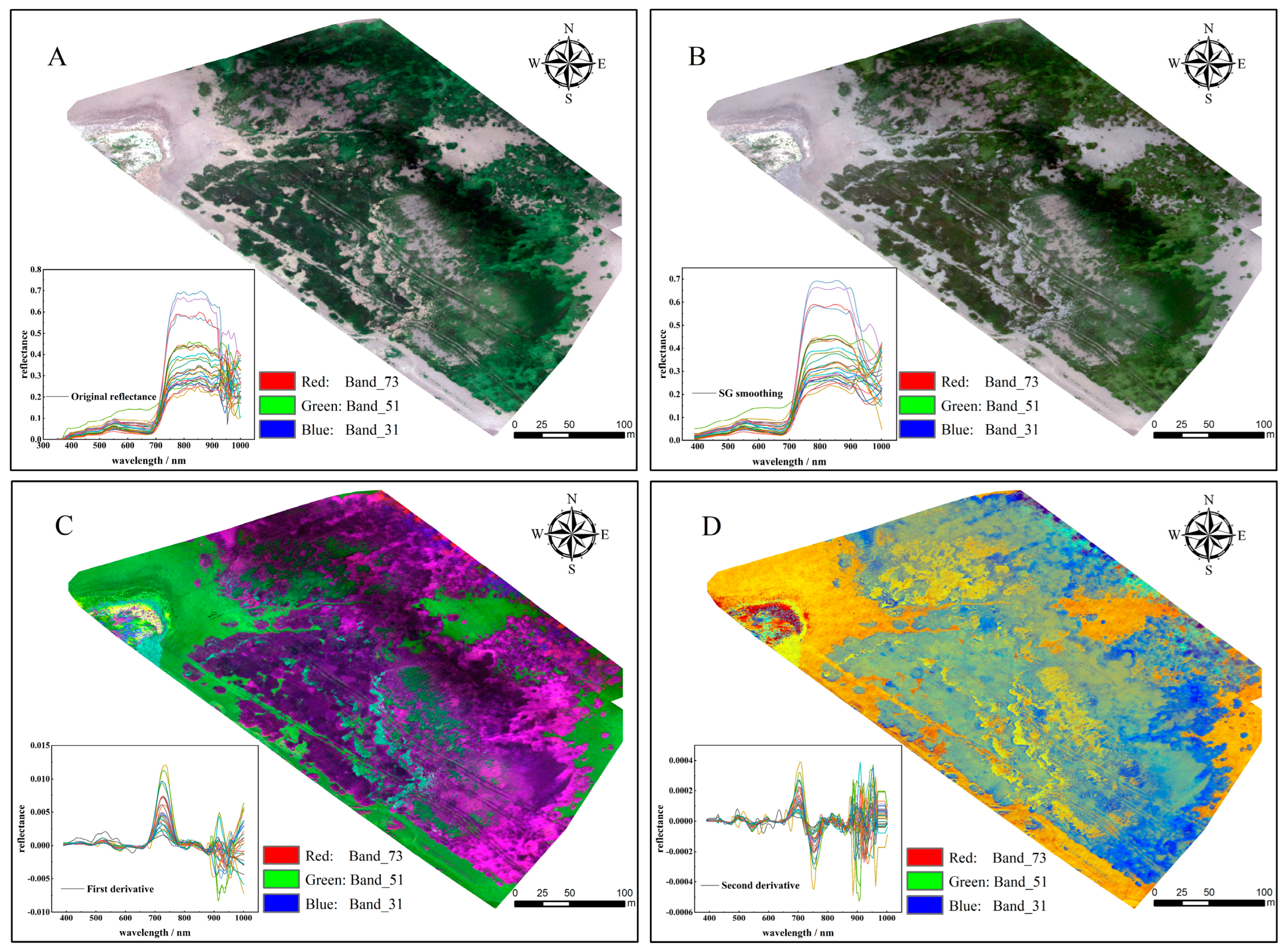
The UAV flight missions were conducted between 11:00 and 13:00 local time on days with clear sky and low wind. Whiteboard calibration was carried out before the flight. The flight altitude, flight speed, forward overlap, and sideward overlap of the UAV were set to 80 m, 6 m/s, 80%, and 80%, respectively. After acquiring the UAV hyperspectral image, image mosaicking and radiometric correction were then carried out. According to the GPS location information of the LAI sampling area, we extracted spectral reflectance from the hyperspectral imagery of the whole plot. We removed the high-noise spectral bands of 350–390 nm caused by the effects of water vapor and the systematic errors of the device. The SG method was further utilized to process the remaining spectral reflectance. To fully explore the potential spectral information, the SG-smoothed original spectral data (OD) were transformed into the FD reflectance and the SD reflectance. Figure 2 shows the canopy reflectance corresponding to FD spectral transformation and SD spectral transformation. The FD of the function f(x) is defined as follows:

$$f^{\mathrm{\prime }}\left(x\right)={\lim }_{t\to 0}\to \frac{f\left(x+t\right)-f\left(x\right)}{t}$$

(1)

Theorem 1.

Here, $t$ is the increment of the independent variable x.

The SD of function $f\left(x\right)$ can be defined as:

$$f^{\mathrm{″}}\left(x\right)={\mathrm{l}\mathrm{i}\mathrm{m}}_{t\to 0}\frac{f\left(x+2t\right)-2f\left(x+t\right)+f\left(x\right)}{t^2}$$

(2)

Figure 2. Images of (A) original hyperspectral; (B) SG smoothing hyperspectral; (C) FD transformation; (D) SD transformation.

Figure 2. Images of (A) original hyperspectral; (B) SG smoothing hyperspectral; (C) FD transformation; (D) SD transformation.

2.2.3. Band Combination Index and Spectral Indices

The basic principle of the BCI method is to combine any three bands to construct the SIs and to perform linear correlation analysis with the LAI to achieve the optimal SIs by comparing correlation coefficients. We further performed spectral transformation on the OD to enhance its sensitivity features with regard to the LAI, and the BCI method was utilized to screen the band combinations after each spectral transformation. The SIs selected using this method provide more abundant spectral information and have a great sensitivity to the LAI of S. alterniflora, and they can better capture the changes in physiological characteristics such as plant leaf structure and, thus, estimate the LAI more accurately. After optimization, the selected SIs have high stability, and the reliability of the prediction model is improved. Referring to previous studies, ESI, MCARI, SIPI, TSI, and NSI perform well in predicting the LAI. Therefore, in this study, these five SIs were built based on the OD, FD, and SD spectral data, respectively (

Table 1. The three-band combination SIs.

Band Combination Type	Spectral Indices	Formula	Source
Three-band spectral indices	ESI	2.5 × (Rk − Rj)/(Rk + 6 × Rj − 7.5 × Ri + 1)	[44]
	NSI	(Rk − Rj)/Ri	[45]
	TSI	0.5 × (120 × (Rk − Ri) − 200 × (Rj − Ri))	[46]
	SIPI	(Rk − Ri)/(Rk − Rj)	[47]
	MCARI	((Rk − Rj) − 0.2 × (Rk − Ri)) × Rk/Rj	[48]

). The constructed OD SIs, FD SIs, and SD SIs were then used as input variables, respectively, to predict the LAI. These new three-band SIs captured vegetation information that could not be covered by the traditional reflectance vegetation indices, which enhanced the sensitivity to LAI. The above SIs were calculated using Python3.10.

2.3. Model Establishment and Verification

2.3.1. Optimized Support Vector Regression

SVR is based on statistical learning theory and needs no assumptions about LAI distribution [44]. This algorithm uses kernel functions to transform the initial input space into a new feature space with more dimensions, thereby transforming the nonlinear regression problem into a linear relationship [49]. The objective of SVR is to estimate unknown continuous-valued functions using a limited number of noise samples. It makes use of the structure minimization principle, which works well in the generalization of different dataset sizes, particularly if the sample size is not large [50]. When the OSVR model is established, the radial basis function (RBF) method of SVR only requires the optimization of the penalty coefficients of cost and the kernel parameter gamma parameters [32,51]. The correct setting of the meta-parameters (cost and gamma) greatly affects the accuracy of SVR. The value of gamma can influence how many support vectors are used in the regression function. Specifically, fewer support vectors are selected as gamma increases. In contrast, smaller gamma values lead to more “flat” predictions, whilst the cost can establish the balance between the training error and the complexity of the model, in which the larger deviations are tolerated in the optimization. Therefore, regardless of the complexity of the model, the larger cost values aim to decrease the empirical risk. In this way, the model complexity is affected by both cost and gamma values [52,53].

As the penalty coefficients of cost and gamma play an important role in the prediction accuracy of the algorithm, a grid search algorithm was conducted to optimize the values of cost and gamma [49].

$${\hat{y}}_i={\displaystyle \sum }_{i=1}^n\left({\hat{\alpha }}_i-{\alpha }_i\right)\cdot k\left(x,x_i\right)+b$$

(3)

$$b=y_i+ϵ-{\displaystyle \sum }_{i=1}^n\left({\hat{\alpha }}_i-{\alpha }_i\right)\cdot k\left(x,x_i\right)$$

(4)

$$k\left(x,x_i\right)=e^{-\gamma \Vert x,x_i{\Vert }^2}$$

(5)

Theorem 2.

Here,$y_i$ represents the LAI-measured values, ${\hat{y}}_i$ represents the LAI prediction value, ${\alpha }_i$ and ${\hat{\alpha }}_i$ represent the weight, $x$ represents the input vector, $k\left(x,x_i\right)$ represents the kernel function, $b$ represents the constant threshold, $ϵ$ represents deviation, $\gamma$ represents gamma, $n$ represents the number of samples, and $i=1,2,\dots ,n$.

2.3.2. Optimized Random Forest Regression

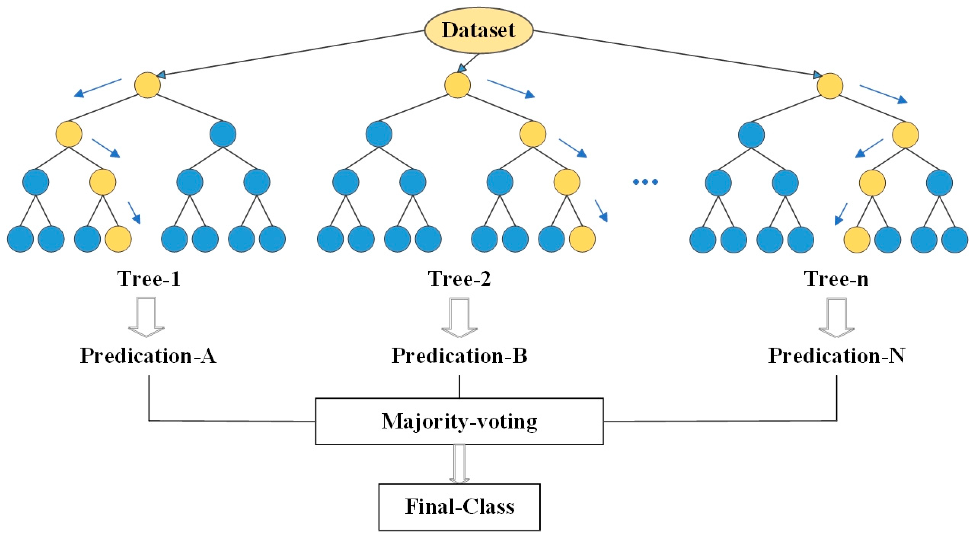
RFR is an integrated learning method that takes the decision tree as the basic learner [54]. It extracts several samples from the original samples and constructs several decision trees by using a bootstrapping method. Then, the average of all the predicted values in the decision tree is taken as the final result (Figure 3); this significantly improves the predictive performance of the decision tree [55]. RFR adds randomness and raises the combined decision tree model’s LAI extrapolation forecast accuracy, which has strong noise resistance, making it difficult to overfit [56]. It successfully handles nonlinear relationships and interactions between features without making any assumptions about the distribution of the input dataset [57]. This is needed to fine-tune the ntree and mtry parameters in order to achieve an excellent performance of RFR. The mtry parameter determines the number of variables that are available and randomly sampled as candidates at each split [58]. Increasing the mtry can enhance the strength of each tree; however, the model will be overfitted at the same time. Conversely, an mtry which is too small reduces the learning ability of the model, which can result in poor generalization performance. In addition, ntree refers to the number of decision trees in the RFR model [59]. The more trees that are grown in the forest, the more reliable and accurate the prediction will be. However, higher computational strain may result from more trees. The estimation accuracy can no longer be raised after a certain point since the generalization error converges as the number of trees grows [60]. By tuning the mtry and ntree parameters and using a grid search to further fine-tune them, better prediction results can be achieved. This approach reduces the out-of-bag (OOB) error value and improves the model accuracy [61].

2.3.3. Optimized Extreme Gradient Boosting Regression

XGBoostR is derived from the gradient-boosting decision tree and is enhanced on top of it [26]. The algorithm is a weighted iterative method to generate decision trees. It fits the first predicted residual by continuously forming a new decision tree to reduce the residual of the measured value and the predictions so as to enhance the model’s fitting ability with difficult-to-predict samples [62]. The advantage of XGBoostR is that it does not need to choose the specific form of the loss function; the leaf-splitting optimization calculation can be performed by relying only on the value of the input data. The loss function is selected according to the need, and the complexity of the model is controlled by adding regular terms to the loss function; this method is conducive to the prevention of overfitting and the improvement of the generalization ability of the model [63]. When the XGBoostR algorithm was employed in the prediction, the following parameters were adjusted through the grid search method to make the model give its best performance. nrounds refers to the number of iterations in training. Underfitting can occur when the nrounds are too low, as this weakens the model and prevents it from performing to its full learning potential. However, excessively high nrounds will lead to overfitting; max_depth is the maximum depth of an individual tree. With the increase in tree depth, the tree model has a stronger fitting ability, but it is more likely to be prone to overfitting; eta determines the updated degree of the model in each iteration. Gamma is the minimum loss reduction required to split a node of the tree; colsample_bytree indicates the random selection of a certain proportion of sample characteristics when building each tree; min_child_weight refers to the minimum sum of the instance weights needed from the leaf nodes to avoid overfitting; subsample means the sampling rate of all the training samples.

2.3.4. Model Verification

The model was trained using the training data and applied to the testing data for prediction. The coefficient of determination (R²), the root mean square error (RMSE), and the residual prediction deviation (RPD) were used as the evaluation indices of the model performance. R² represents the degree to which the model fits the data, and RMSE reflects the dispersion degree of the measured values near the regression line. The larger the R², the smaller the RMSE and the higher the level of model-estimation accuracy that is shown. The RPD can better indicate the prediction ability. When the RPD < 1.4, it indicates that the model cannot estimate the LAI; when 1.4 < RPD ≤ 2.0, the predictive ability of the model is relatively reliable; when RPD > 2.0, the model has excellent prediction ability [42]. The formulas are as given below.

$$R^2=\frac{\sum _{i=1}^n{\left({\hat{y}}_i-\overline{y}\right)}^2}{\sum _{i=1}^n{\left(y_i-\overline{y}\right)}^2}$$

(6)

$$RMSE=\sqrt{\frac{\sum _{i=1}^n{\left({\hat{y}}_i-y_i\right)}^2}{n}}$$

(7)

$$RPD=\frac{SD}{RMSE}$$

(8)

Theorem 3.

Here,  $y_i$ indicates the measured values of LAI,  ${\hat{y}}_i$ indicates the prediction of LAI,  $\stackrel{-}{y}$ indicates the average measured values of LAI,  $n$ indicates the number of samples,  $i=1,2,\dots ,n$ , and  $SD$ is the standard deviation of the measured value.

2.4. Methodology

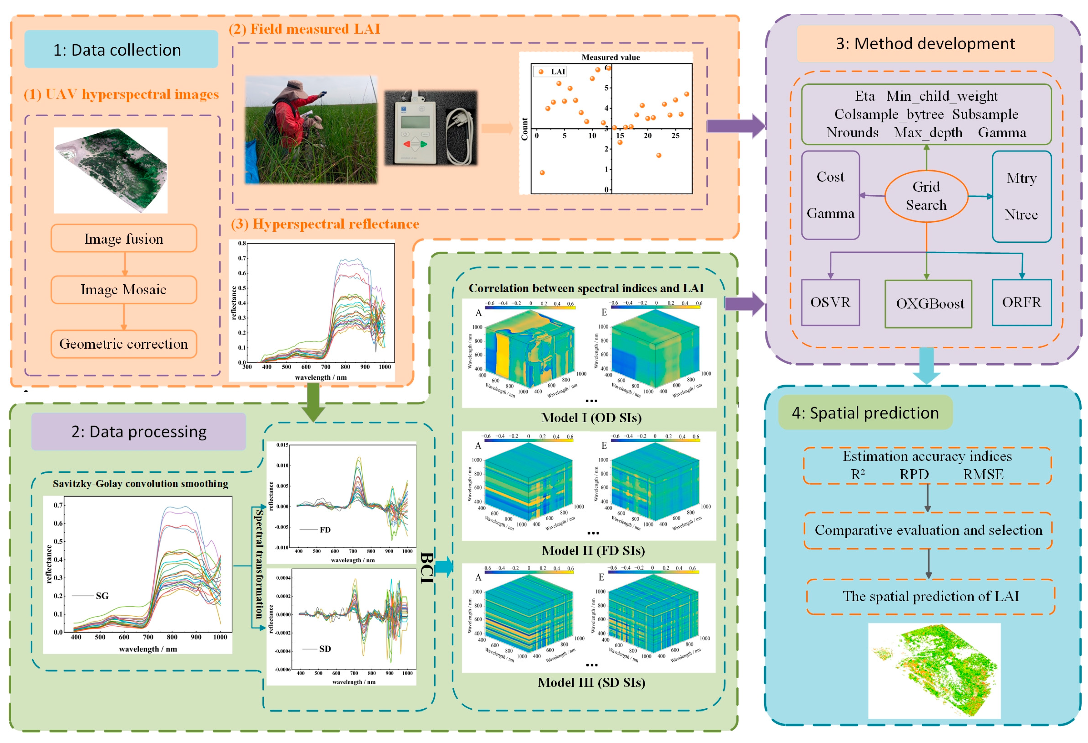
To better-understand the process of LAI model estimation, a methodological analysis framework was established (Figure 4). This study classified the framework into four main parts: (1) Data collection: Three kinds of data were used, including LAI field measurements, UAV hyperspectral imagery, and spectral reflectance derived from UAV hyperspectral images. The LAI and UAV hyperspectral imagery was produced in the field, and the spectral reflectance of S. alterniflora was extracted from the UAV imagery corresponding to the location of the LAI sampling points. (2) Data preprocessing: The methods of spectral reflectance underwent SG smoothing and employed two further spectral transformations to reduce the spectral noise. Then, a correlation analysis between the LAI and the spectral reflectance based on the BCI methods was carried out to select the bands sensitive to LAI, and the SIs with optimal characteristic band combinations were constructed to predict the LAI. (3) Model development: Model I, Model II, and Model III used OD SIs, FD SIs, and SD SIs, respectively, as input variables. Three ML algorithms, OSVR, ORFR, and OXGBoostR, were implemented to establish the LAI prediction model. (4) By comparing the model accuracy of each case, the model with the best accuracy could be selected to invert the LAI of S. alterniflora.

3. Results and Analysis

3.1. Statistical Analysis of LAI

The LAI of S. alterniflora collected in the study area was subjected to statistical analysis, the results of which are summarized in

Table 2. Statistical analysis of S. alterniflora LAI.

Data	Number	Min	Max	Mean	Standard Deviation	Coefficient of Variation
All	27	0.84	5.97	3.87	1.16	29.97%
Train	19	0.84	5.97	3.75	1.27	33.87%
Test	8	3.1	5.89	4.19	0.84	20.05%

. The 27 samples were randomly divided into a training set and a testing set at a ratio of 7:3. The LAI range of S. alterniflora in the study area was roughly 0.84~5.97, while the means of the LAI corresponding to the training set and testing set were 3.75 and 4.19, respectively; the standard deviations of the training data and testing data were 1.27 and 0.84, respectively. The mean value of all the sampling points was 3.87, with a coefficient of variation of 29.97%.

3.2. Spectral Indices Constructed Using BCI Band Selection

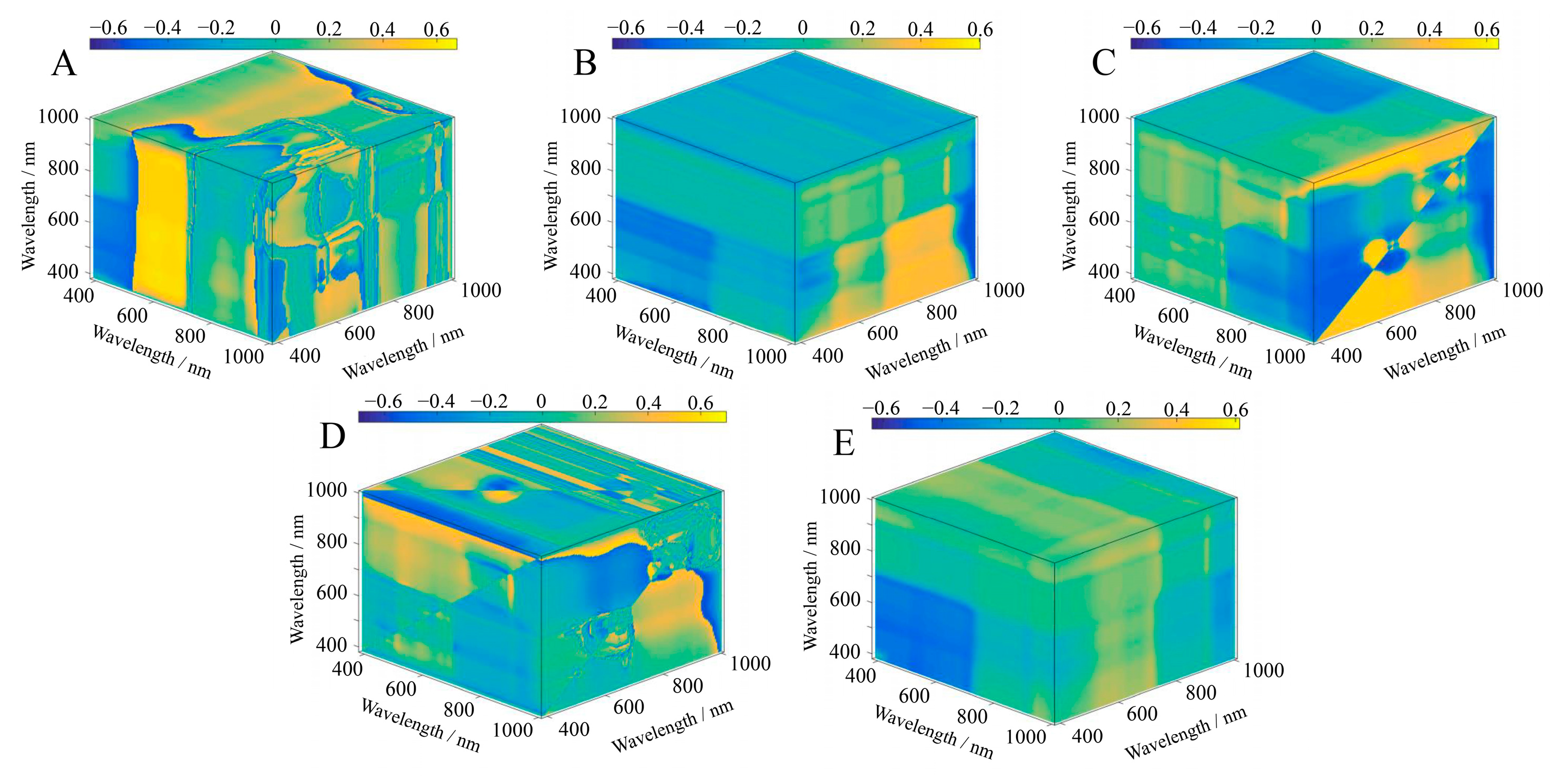
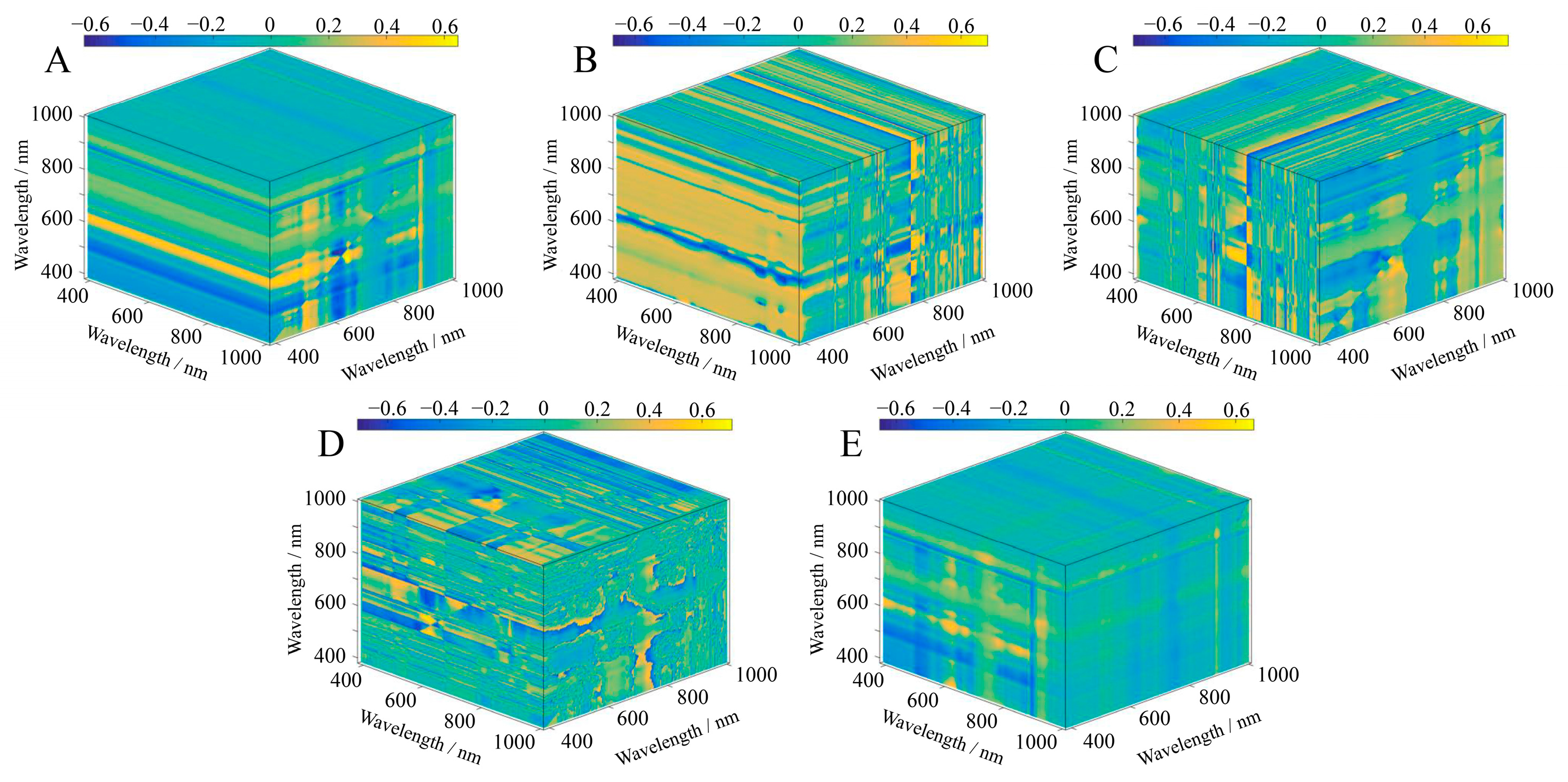
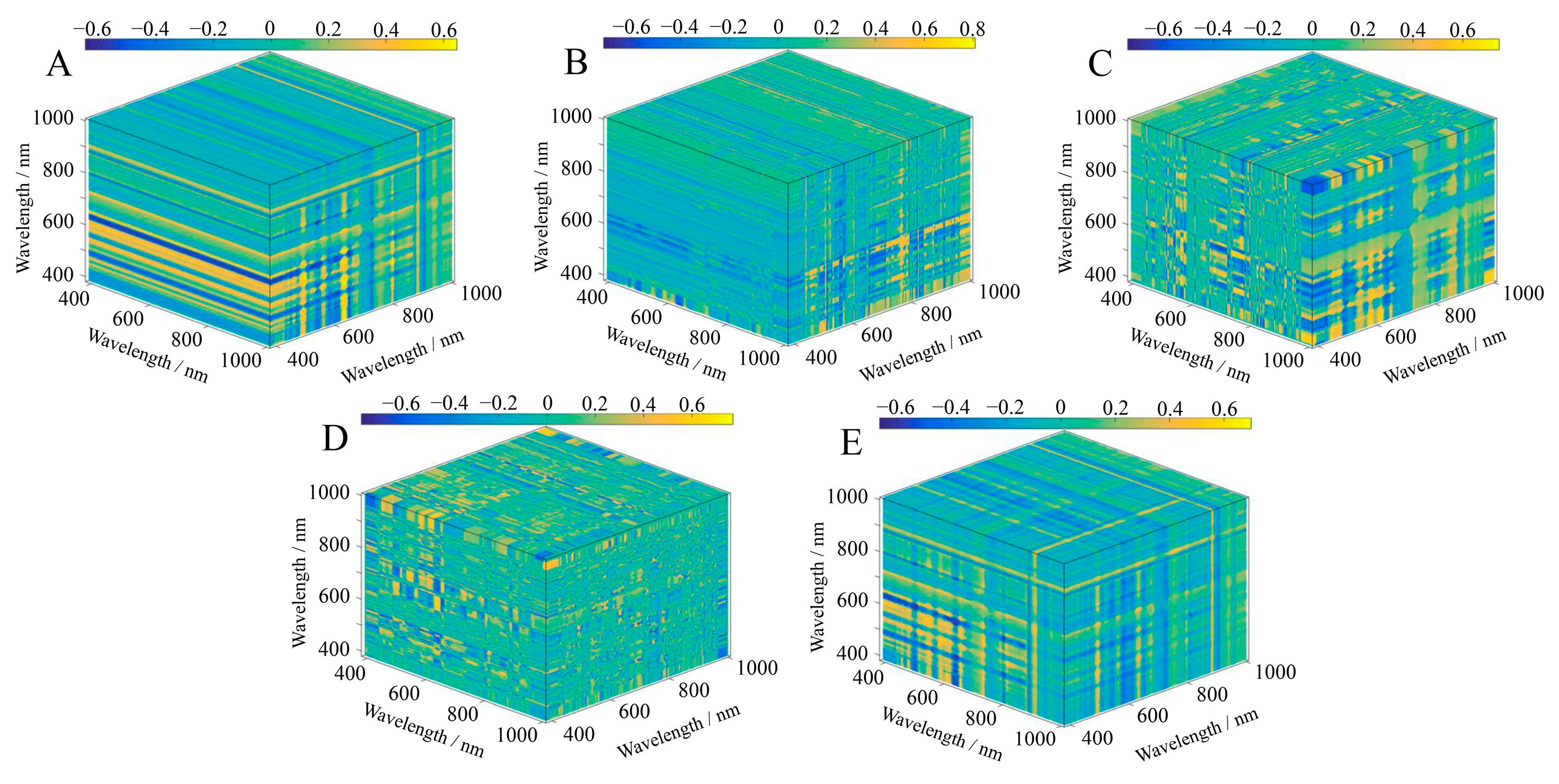
The contour maps show the relationship between the SIs and the LAI of S. alterniflora in three dimensions, and the intensity of the colors corresponds to the strength of the correlation (Figure 5, Figure 6 and Figure 7). A significant correlation was found between the LAI and the five three-band SIs, and all results were significant at the p < 0.01 level (

Table 3. SIs of OD, FD, and SD with the highest correlation with LAI.

Model	Data Type	Optimum Spectral Indices Abbreviation	Correlation Coefficient
Model I	OD Spectral Data	ESI (862 nm 934 nm 962 nm)	0.69 **
		MCARI (650 nm 618 nm 610 nm)	0.62 **
		NSI (902 nm 646 nm 642 nm)	0.64 **
		SIPI (650 nm 642 nm 718 nm)	0.68 **
		TSI (638 nm 630 nm 626 nm)	0.63 **
Model II	FD Spectral Data	ESI (914 nm 598 nm 646 nm)	0.65 **
		MCARI (954 nm 662 nm 514 nm)	0.69 **
		NSI (730 nm 734 nm 642 nm)	0.71 **
		SIPI (538 nm 818 nm 826 nm)	0.71 **
		TSI (566 nm 646 nm 622 nm)	0.66 **
Model III	SD Spectral Data	ESI (886 nm 526 nm 638 nm)	0.65 **
		MCARI (646 nm 606 nm 614 nm)	0.81 **
		NSI (734 nm 606 nm 446 nm)	0.74 **
		SIPI (582 nm 634 nm 794 nm)	0.77 **
		TSI (526 nm 646 nm 650 nm)	0.70 **

** indicates significant at the p < 0.01 level.

). The results also showed that there were differences in the band ranges of the OD, FD, and SD SI band combinations, mainly in the fact that the bands constituting the OD SIs were more concentrated, while the band ranges of the FD SIs and SD SIs included other types of visible light spectra. The bands that built the OD SIs had a wavelength range of 610 nm to 934 nm and were from both the red and near-infrared wavelength ranges (Figure 5). In all the bands involved in the construction of the FD SIs, the wavelengths ranged from 514 nm to 954 nm, and more than two-thirds were located in the red and near-infrared wavelength ranges (Figure 6). Furthermore, we found that in the wavelength that built the SD SIs, 73.3% were in the red and near-infrared range of 600 nm to 886 nm, of which 26.7% were in the blue, green, and yellow range of 446 nm to 600 nm (Figure 7). According to these findings, the spectral transformation enlarges the wavelength range of the band combinations of SIs. Except for ESI, the correlation between the SIs constructed with spectral reflectance after spectral transformation and the LAI increased. We calculated the ranges of the absolute correlation between the LAI and SIs as being from 0.62 to 0.69 for the OD SIs and 0.65 to 0.71 for the FD SIs. After the FD spectral transformation, the correlation of FD–MCARI was improved by 11.29% compared with OD–MCARI, which had the highest correlation increase. Additionally, the correlation was relatively high between the LAI and the SD SIs, with the highest correlation being that of SD–MCARI (correlation coefficient = 0.81), which was 30.65% higher than that of OD–MCARI. Additionally, the highest correlations with the LAI in the OD SIs and SD SIs were, respectively, OD–ESI and SD–MCARI, whereas in the FD SIs they were FD–NSI and FD–SIPI. The maximum correlation coefficients were 11.29%, 9.23%, and 24.6% higher than the lowest correlation coefficients between the SIs of OD, FD, and SD, and LAI.

3.3. Model Establishment and Comparison

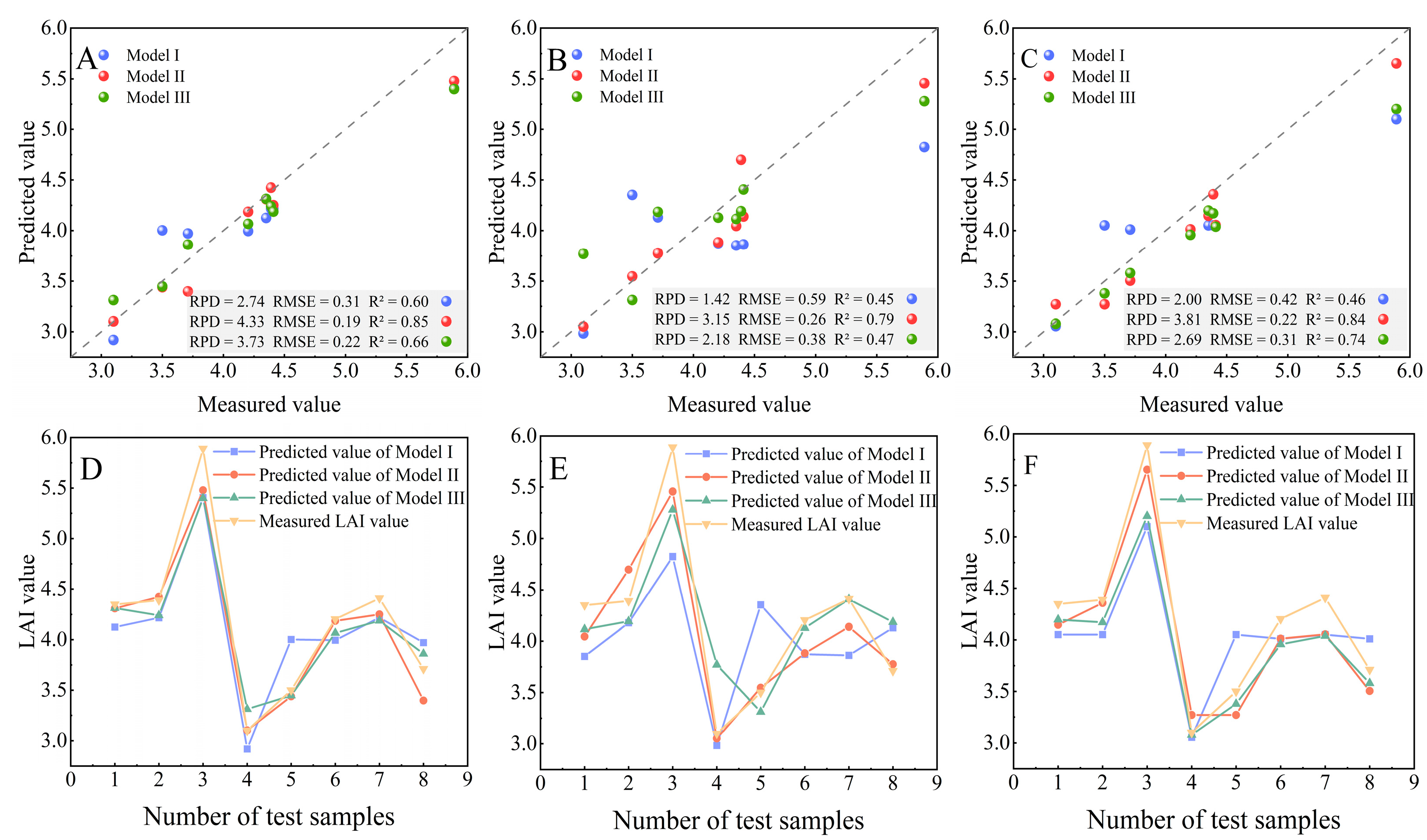
The performances of three ML algorithms, including ORFR, OSVR, and OXGBoostR, based on the SIs of OD, FD, and SD for predicting the LAI, are displayed in Figure 8. The results of the grid search method for the hyperparameter optimization are shown in

Table 4. OSVR and ORFR model optimized parameters.

Transform Form	OSVR		ORFR
	Cost	Gamma	Ntree	Mtry
OD	2	0.02	500	4
FD	9	0.01	500	5
SD	2	0.02	500	3

and

Table 5. OXGBoostR model optimized parameters.

Transform Form	OXGBoostR
	Nrounds	Max_depth	Eta	Gamma	Colsample_bytree	Min_child_ weight	Subsample
OD	40	1	0.1	1	0.6	2	0.6
FD	50	1	0.1	0.05	0.8	2	0.6
SD	40	5	0.1	0.1	0.8	2	0.6

. According to the performance of the modeling, the different methods and SI band combinations have a large impact. For the ORFR and OXGBoostR algorithms, Model I (R² = 0.60 vs. R² = 0.46, respectively) and Model II (R² = 0.85 vs. R² = 0.84, respectively) were better-estimated by the ORFR algorithm, proving that the ORFR algorithm is superior to OXGBoostR for estimating the LAI using OD SIs and FD SIs. The OXGBoostR method, however, outperformed ORFR in Model III (R² = 0.66 vs. R² = 0.74, respectively), revealing that it is better-suited than ORFR for estimating the LAI utilizing SD SIs. Among the three ML methods, whether using OD SIs or spectral transformation SIs as input variables, the OSVR algorithms possess the lowest estimation precision for the LAI.

Model II outperformed Model I and Model III in comparison with various combinations of independent variables. The R² values of Model I and Model II in the ORFR method were 0.01 and 0.14 higher than those of OXGBoostR, respectively. However, in Model III, the R² of the ORFR algorithm was 0.08 smaller than that of OXGBoostR, proving that when estimating LAI utilizing the ORFR and OXGBoostR methods, the FD spectral data have a greater predictive performance than the OD spectral data and SD spectral data, while the SD spectral data have a better predictive performance than the OD spectral data. In addition, the R² values of Model II and Model III were 75.6% (from 0.45 to 0.79) and 4.44% (from 0.45 to 0.47) greater than that of Model I, respectively. For the models built using the OSVR method, this shows that the spectral transformation data outperform the OD spectral data. When compared with the OD spectral data, the spectral transformation data can increase prediction accuracy, and each type of hyperspectral data transformation possesses a varied level of improvement with regard to the precision of the model. For example, when the FD SIs were used instead of the OD SIs, the maximum R² increased by 82.61%. When the SD SIs were used instead of the OD SIs, the maximum R² increased by 60.87%. This suggests that useful information other than the OD spectral data is included in the data after spectral transformation. These improvements are the same for all three ML algorithms.

Model II showed good performance among the three ML methods in predicting the LAI. For example, when compared with Model I, the R² value of Model II, based on the ORFR approach, improved from 0.60 to 0.85; this represented an improvement over Model III of 30.30%. Model II was based on three methods, with R² values of 0.85, 0.79, and 0.84 for the ORFR, OSVR, and OXGBoostR methods, respectively, which can account for the variations in the LAI of 85.0%, 79.0%, and 84.0%, respectively. The fitted straight line between the measured value and the predicted value was closer to the 1:1 line, and the LAI predicted using the ORFR method was closest to the measured value, according to the distribution of the measured value and the predicted value scatterplot (Figure 8), with the OXGBoostR and OSVR being relatively scattered.

3.4. Spatial Distribution Pattern of LAI

The method based on ORFR combined with FD SIs was selected to estimate the LAI of S. alterniflora, and the spatial distribution of LAI in the study area is displayed in Figure 9. The distribution maps showed a significant spatial heterogeneity for the LAI, with a lower LAI in the vicinity of S. alterniflora and the tidal flat and a higher LAI in the coastal regions. The LAI of striped S. alterniflora had a relatively high trend on the land side parallel to the shoreline. Patches of S. alterniflora could still be found in the research region, and the LAI was not very high (Figure 9A). Locally, S. alterniflora at the border with the tidal flat showed a lower LAI (Figure 9C); however, the LAI was higher at the confluence of S. alterniflora’s flourishing growth area and withering area than it was at the junction of the tidal flat (Figure 9D). This may be related to the presence of more S. alterniflora in the healthy growth stage in the transition zone between the vigorously growing area and the withered area; due to S. alterniflora’s greater proximity to the ground and its shorter plant height, as seen in Figure 9E, S. alterniflora had a lower LAI overall. According to the statistical study, the vast majority of the pixels in the coastal areas had LAI values between 3.2 and 5.0 (Figure 9B). The apex of the distribution curve swings towards a higher LAI as we proceed from land to coastal wetlands areas, showing that the LAI in land areas is much lower than that in coastal wetland areas.

4. Discussion

4.1. Accuracy and Influencing Factors of LAI Prediction Models

The vegetation spectrum is a comprehensive reflection of various vegetation properties, which are affected by the factors of plant canopy structure (leaf orientation and shade) and soil background, among others [64]. Previous studies have shown that spectral transformation can significantly improve the sensitivity of the vegetation spectrum to LAI [65,66]. Spectral transformation can be used to process spectral data to estimate the LAI of S. alterniflora. Our study reveals that three types of SIs, namely OD SIs, FD SIs, and SD SIs, all influence LAI prediction precision to varied degrees. The accuracy of the model based on the variables constructed from OD and two types of spectral transformation data is different. Due to discrepancies in the enhanced band information of the spectral transformation, the available information found in the data of the transformation is enlarged [67]; this can lead to different LAI prediction capabilities. Compared with Model II, Model III had less precision. This shows that FD SIs have better predictive ability than SD SIs in our typical S. alterniflora plots, which is consistent with earlier findings [58]. Although the SD SIs showed a higher correlation with the LAI, a lower prediction accuracy between the SD SIs and the LAI was detected. This may be due to FD SIs being better-able to capture the nonlinear relationship with the LAI. Meanwhile, the FD transformation can also enhance changes in the spectral information in the visible and near-infrared regions, help lower noise and abiotic interference in spectral data, and display the spectrum absorption characteristic information of the LAI [68]. In contrast, the SD transformation emphasizes high-frequency changes in data that may increase noise and reduce model accuracy [32]. In this study, the use of spectral transformation data to estimate the LAI is illustrated by the increased prediction accuracy gained from the FD SIs, which is consistent with the findings of UMUT [69].

Our results show that different transformation process data and prediction algorithms have a substantial impact on the predictive accuracy of the LAI. In predicting the LAI using three different types of SIs, we found that the ORFR algorithm performed best at predicting the LAI using OD and FD SIs, while OXGBoostR performed best at predicting the LAI using SD SIs. Therefore, when employing different models, it is crucial to calibrate and assess competitive estimation models based on specific experimental datasets. The RFR method performed better in terms of prediction accuracy than the XGBoostR and SVR methods; this result is consistent with that of previous studies [70]. However, Zhang et al. adopted RFR, SVR, and XGBoostR to invert the LAI in a soybean survey region and found that XGBoostR had the optimal accuracy at the flowering stage; RFR performed best at the podding stage and mature stage; and SVR performed relatively poorly during the three periods [25]. There is no consistent conclusion on the model prediction ability of the RFR, SVR and XGBoostR methods; this may be related to the sampling time of the LAI or the different vegetation types. It appears that no single ML approach is suitable for all ecosystems; thus, it is crucial to choose many approaches based on different regions and input variables. Many collinearity problems for unbalanced datasets and the reduction in data mistakes can be solved by the model created by the ORFR method, which has strong noise tolerance and generalization capacity [38]. In comparison, the OXGBoostR method introduced more controllable parameters that optimized the algorithm for the problem scenario and customized the loss function through the gradient boosting framework, improving the ability to solve generic problems [41].

The ORFR method based on Model II had the highest estimation accuracy of all the estimating models and could account for 85.0% of the variability in the LAI. This may be because the FD SIs emphasize the information change in the spectrum and provide richer characteristic information. This feature helps ORFR to capture subtle changes in the spectral data, while the risk of overfitting is reduced by ORFR through the random selection of subsamples and features [38]. Additionally, OSVR and OXGBoostR are more noise-sensitive than ORFR. These characteristics may have enabled ORFR to outperform OSVR and OXGBoostR in this study’s prediction results. In addition, compared with the LAI predictions made by other researchers, our estimation model has greater accuracy. For instance, using GF-5, Chen et al. created an RFR model that can explain 82.8% of the variation in the LAI [71]. Upreti et al. used data from Sentinel-2 to construct a least squares linear regression (LSLR) model to predict the LAI, with an R² value of 0.78 [72]. Although satellite remote sensing images have wide coverage and rich attribute information, they have poor image resolution and cannot be matched with LAI sampling points; thus, they cannot improve the inversion of a small range of LAIs. When compared with the use of satellite remote sensing images, the high-precision UAV hyperspectral image has an important influence on the improvement of the accuracy of the model.

4.2. Bands Screened Using the BCI Method

The traditional reflectance vegetation indices only used limited band information and could not fully extract the best spectral bands, which affected the prediction accuracy of the LAI [34]. To obtain vegetation reflection information to the maximum extent and to reduce the influence of external factors, Pei and Kong et al. confirmed the effectiveness of the BCI method in monitoring the LAI and chlorophyll content of rice, respectively [30,33]. Fu et al. demonstrated that the model precision of prediction could be effectively improved by using BCI to optimize the parameters of NDVI-like and band depth [73]. According to previous studies, the BCI method is a useful method for screening hyperspectral characteristic bands, and it can address the issues of hyperspectral information redundancy and improve spectral modeling accuracy.

The correlation analysis matrix between characteristic band combinations and the LAI under various spectral transformations was established in this study using the BCI algorithm. Each SI of the best band combinations showed a highly significant correlation with the LAI, and the characteristic bands screened using the BCI method mainly focused on the red and near-infrared band ranges. Previous studies have also explained the importance of the red band and the near-red band in predicting the LAI. For example, the R² contour map was used by Shinya et al. to screen out the characteristic bands with the highest R² of the LAI, and they found that the characteristic bands were mainly concentrated in the red band and the near-infrared band [74]. Li et al. optimized the selection of spectral features and estimated the LAI through the preferred SIs; the red edge–NIR spectral region was the range that was most sensitive to the LAI [75]. Our research shows that, when affected by the band span of the three-band SIs, the significant correlation bands of the LAI also indicated significant bands between blue bands and green bands. It is possible that this occurred because of the relatively much greater sensitivity of the blue and green bands to the effect of chlorophyll content when compared with the red and near-infrared bands [76]. In general, various bands selected with the BCI method play an important role in LAI estimation. By comprehensively utilizing the information on these bands of SIs, LAI inversion can be obtained more accurately, and the growth state and health status of the vegetation can be further understood.

4.3. Spatial Distribution of LAI

The predicted spatial distribution of the LAI in this study was consistent with the actual spatial distribution, which further indicated that the results of this study were reasonable. Regarding the results of the prediction, the spatial distribution of the LAI based on the ORFR Model II revealed that S. alterniflora had strong spatial heterogeneity, and the areas with relatively low LAIs were mainly concentrated in the areas bordering the tidal flat. A few S. alterniflora LAIs ranged from 0.87 to 1.53 and were mainly distributed in the intersection of S. alterniflora and the tidal flat in the southeast of the study area. This may be related to the negative effects of seafood harvesting activities by humans on the mudflat near the shore on the growth of S. alterniflora (Figure 10A). The proportion of regions with a relatively low LAI on the landward side was relatively large, mostly between 1.54 and 2.85; this was caused by the short invasion time and low plant height of S. alterniflora in this region (Figure 10B). The high-value LAI areas were primarily found in the middle and seaward part of the study area, where S. alterniflora grew well and had high photosynthetic capacity, with an LAI range of 3.20 to 5.00. There was no species competition, the invasion duration was rather long, and the region was only weakly affected by human activities. All of the above indicated that the LAI of S. alterniflora might be related to human activities, invasion time, and plant height.

5. Conclusions

This study compared the performances of three ML methods, namely ORFR, OSVR, and OXGBoostR, in conjunction with the OD, FD, and SD SIs that were screened using the BCI method to evaluate the LAI. The results show the following:

• The spectral transformation of spectra can effectively improve the accuracy of the model estimations; among these, the precision had the greatest improvement with the FD transformation. The ORFR, OSVR, and OXGBoostR methods demonstrated R² values of 0.85, 0.79, and 0.84, respectively.
• By applying the BCI method to obtain SIs as the independent variables to predict the LAI, good prediction results can be obtained. Moreover, the band combinations that are significantly correlated with the LAI screened using the BCI method are mainly concentrated in the red band and near-infrared band range, and very few are in the blue and green band range.
• The prediction accuracy of the ORFR algorithm combined with the OD and FD SIs is, respectively, superior to that of OSVR and OXGBoostR, and OXGBoostR performs best when the SD SIs combine three ML algorithms. The optimal model was constructed by adopting the ORFR algorithm combined with FD SIs, with an R² of 0.84, an RMSE of 0.19, and an RPD of 4.33.
• The LAI predicted using the ORFR method ranged from 0.87 to 6.017. There was a spatial difference between the higher LAI on the seawall side and the lower LAI at the junction of S. alterniflora and the tidal flats.

References

1. Yuan, Y.; Tang, X.; Liu, M.; Liu, X.; Tao, J. Species Distribution Models of the Spartina alterniflora Loisel in Its Origin and Invasive Country Reveal an Ecological Niche Shift. Front. Plant Sci. 2021, 12, 738769. [Google Scholar] [CrossRef] [PubMed]
2. Song, L.; Wang, Q.; Wang, P.; Wu, J. Benthic bacterial communities and bacteria–environment interactions after Kandelia obovata introduction and Spartina alterniflora invasion in Yueqing Bay, China. Reg. Stud. Mar. Sci. 2023, 58, 102787. [Google Scholar] [CrossRef]
3. Matsuda, R.; Yamada, K.; Hayasaka, D.; Henmi, Y. Effects of salinity, temperature, and immersion conditions on seed germination of invasive Spartina alterniflora Loisel (smooth cordgrass) in Japan. Reg. Stud. Mar. Sci. 2023, 57, 102738. [Google Scholar] [CrossRef]
4. Huang, Y.; Liu, Z.; Zheng, G.; Zhao, C. Identification of Spartina alterniflora habitat expansion in a Suaeda salsa dominated coastal wetlands. Ecol. Indic. 2022, 145, 109704. [Google Scholar] [CrossRef]
5. Wang, B.; Lin, X. Exotic Spartina alterniflora invasion enhances sediment N-loss while reducing N retention in mangrove wetland. Geoderma 2023, 431, 116362. [Google Scholar] [CrossRef]
6. Zhu, W.; Ren, G.; Wang, J.; Wang, J.; Hu, Y.; Lin, Z.; Li, W.; Zhao, Y.; Li, S.; Wang, N. Monitoring the Invasive Plant Spartina alterniflora in Jiangsu Coastal Wetland Using MRCNN and Long-Time Series Landsat Data. Remote Sens. 2022, 14, 2630. [Google Scholar] [CrossRef]
7. Xia, S.; Wang, W.; Song, Z.; Kuzyakov, Y.; Guo, L.; Van Zwieten, L.; Li, Q.; Hartley, I.P.; Yang, Y.; Wang, Y.; et al. Spartina alterniflora invasion controls organic carbon stocks in coastal marsh and mangrove soils across tropics and subtropics. Glob. Chang. Biol. 2021, 27, 1627–1644. [Google Scholar] [CrossRef] [PubMed]
8. Han, X.; Wang, Y.; Ke, Y.; Liu, T.; Zhou, D. Phenological heterogeneities of invasive Spartina alterniflora salt marshes revealed by high-spatial-resolution satellite imagery. Ecol. Indic. 2022, 144, 109492. [Google Scholar] [CrossRef]
9. Nandan, R.; Bandaru, V.; He, J.; Daughtry, C.; Gowda, P.; Suyker, A.E. Evaluating Optical Remote Sensing Methods for Estimating Leaf Area Index for Corn and Soybean. Remote Sens. 2022, 14, 5301. [Google Scholar] [CrossRef]
10. Chenwei, N.; Lei, S.; Zhenhai, L.; Xiaobin, X.; Dameng, Y.; Shaokun, L.; Xiuliang, J. A comparison of methods to estimate leaf area index using either crop-specific or generic proximal hyperspectral datasets. Eur. J. Agron. 2023, 142, 126664. [Google Scholar] [CrossRef]
11. De Bock, A.; Belmans, B.; Vanlanduit, S.; Blom, J.; Alvarado-Alvarado, A.A.; Audenaert, A. A review on the leaf area index (LAI) in vertical greening systems. Build. Environ. 2023, 229, 109926. [Google Scholar] [CrossRef]
12. Liang, L.; Di, L.; Zhang, L.; Deng, M.; Qin, Z.; Zhao, S.; Lin, H. Estimation of crop LAI using hyperspectral vegetation indices and a hybrid inversion method. Remote Sens. Environ. 2015, 165, 123–134. [Google Scholar] [CrossRef]
13. Pu, J.; Yan, K.; Gao, S.; Zhang, Y.; Park, T.; Sun, X.; Weiss, M.; Knyazikhin, Y.; Myneni, R.B. Improving the MODIS LAI compositing using prior time-series information. Remote Sens. Environ. 2023, 287, 113493. [Google Scholar] [CrossRef]
14. Caballero, G.; Pezzola, A.; Winschel, C.; Casella, A.; Angonova, P.S.; Rivera-Caicedo, J.P.; Berger, K.; Verrelst, J.; Delegido, J. Seasonal Mapping of Irrigated Winter Wheat Traits in Argentina with a Hybrid Retrieval Workflow Using Sentinel-2 Imagery. Remote Sens. 2022, 14, 4531. [Google Scholar] [CrossRef]
15. Zhang, Y.; Yang, J.; Du, L. Analyzing the Effects of Hyperspectral ZhuHai-1 Band Combinations on LAI Estimation Based on the PROSAIL Model. Sensors 2021, 21, 1869. [Google Scholar] [CrossRef]
16. Tomíček, J.; Mišurec, J.; Lukeš, P.; Potůčková, M. Retrieval of Harmonized LAI Product of Agricultural Crops from Landsat OLI and Sentinel-2 MSI Time Series. Agriculture 2022, 12, 2080. [Google Scholar] [CrossRef]
17. Qiao, L.; Zhao, R.; Tang, W.; An, L.; Sun, H.; Li, M.; Wang, N.; Liu, Y.; Liu, G. Estimating maize LAI by exploring deep features of vegetation index map from UAV multispectral images. Field Crop. Res. 2022, 289, 108739. [Google Scholar] [CrossRef]
18. Cheng, Q.; Xu, H.; Fei, S.; Li, Z.; Chen, Z. Estimation of Maize LAI Using Ensemble Learning and UAV Multispectral Imagery under Different Water and Fertilizer Treatments. Agriculture 2022, 12, 1267. [Google Scholar] [CrossRef]
19. Croci, M.; Impollonia, G.; Marcone, A.; Antonucci, G.; Letterio, T.; Colauzzi, M.; Vignudelli, M.; Ventura, F.; Anconelli, S.; Amaducci, S. RTM Inversion through Predictive Equations for Multi-Crop LAI Retrieval Using Sentinel-2 Images. Agronomy 2022, 12, 2835. [Google Scholar] [CrossRef]
20. Wang, J.; Si, H.; Gao, Z.; Shi, L. Winter Wheat Yield Prediction Using an LSTM Model from MODIS LAI Products. Agriculture 2022, 12, 1707. [Google Scholar] [CrossRef]
21. Zhang, M.; Ustin, S.L.; Rejmankova, E.; Sanderson, E.W. Monitoring Pacific coast salt marshes using remote sensing. Ecol. Appl. 1997, 7, 1039–1053. [Google Scholar] [CrossRef]
22. Guo, A.; Huang, W.; Dong, Y.; Ye, H.; Ma, H.; Liu, B.; Wu, W.; Ren, Y.; Ruan, C.; Geng, Y. Wheat Yellow Rust Detection Using UAV-Based Hyperspectral Technology. Remote Sens. 2021, 13, 123. [Google Scholar] [CrossRef]
23. Caballero, G.; Pezzola, A.; Winschel, C.; Casella, A.; Angonova, P.S.; Orden, L.; Berger, K.; Verrelst, J.; Delegido, J. Quantifying Irrigated Winter Wheat LAI in Argentina Using Multiple Sentinel-1 Incidence Angles. Remote Sens. 2022, 14, 5867. [Google Scholar] [CrossRef]
24. Ma, Y.; Zhang, Q.; Yi, X.; Ma, L.; Zhang, L.; Huang, C.; Zhang, Z.; Lv, X. Estimation of Cotton Leaf Area Index (LAI) Based on Spectral Transformation and Vegetation Index. Remote Sens. 2021, 14, 136. [Google Scholar] [CrossRef]
25. Zhang, Y.; Yang, Y.; Zhang, Q.; Duan, R.; Liu, J.; Qin, Y.; Wang, X. Toward Multi-Stage Phenotyping of Soybean with Multimodal UAV Sensor Data: A Comparison of Machine Learning Approaches for Leaf Area Index Estimation. Remote Sens. 2022, 15, 7. [Google Scholar] [CrossRef]
26. Sudu, B.; Rong, G.; Guga, S.; Li, K.; Zhi, F.; Guo, Y.; Zhang, J.; Bao, Y. Retrieving SPAD Values of Summer Maize Using UAV Hyperspectral Data Based on Multiple Machine Learning Algorithm. Remote Sens. 2022, 14, 5407. [Google Scholar] [CrossRef]
27. Colovic, M.; Yu, K.; Todorovic, M.; Cantore, V.; Hamze, M.; Albrizio, R.; Stellacci, A.M. Hyperspectral Vegetation Indices to Assess Water and Nitrogen Status of Sweet Maize Crop. Agronomy 2022, 12, 2181. [Google Scholar] [CrossRef]
28. Datta, D.; Paul, M.; Murshed, M.; Teng, S.W.; Schmidtke, L. Soil Moisture, Organic Carbon, and Nitrogen Content Prediction with Hyperspectral Data Using Regression Models. Sensors 2022, 22, 7998. [Google Scholar] [CrossRef]
29. Fang, W.; Zhu, H.; Li, S.; Ding, H.; Bi, R. Rapid Identification of Main Vegetation Types in the Lingkong Mountain Nature Reserve Based on Multi-Temporal Modified Vegetation Indices. Sensors 2023, 23, 659. [Google Scholar] [CrossRef]
30. Kong, Y.; Wang, L.; Feng, H.; Xu, Y.; Liang, L.; Xu, L.; Yang, X.; Zhang, Q. Leaf Area Index Estimation Based on UAV Hyperspectral Band Selection. Spectrosc. Spectr. Anal. 2022, 42, 933–939. [Google Scholar] [CrossRef]
31. Liu, X.; Wang, H.; Cao, Y.; Yang, Y.; Sun, X.; Sun, K.; Li, Y.; Zhang, J.; Pei, Z. Comprehensive growth index monitoring of desert steppe grassland vegetation based on UAV hyperspectral. Front. Plant Sci. 2022, 13, 1050999. [Google Scholar] [CrossRef]
32. Yang, X.; Huang, J.; Wu, Y.; Wang, J.; Wang, P.; Wang, X.; Huete, A.R. Estimating biophysical parameters of rice with remote sensing data using support vector machines. Sci. China Life Sci. 2011, 54, 272–281. [Google Scholar] [CrossRef]
33. Pei, H.; Feng, H.; Li, C.; Jin, X.; Li, Z.; Yang, G. Remote sensing monitoring of winter wheat growth with UAV based on comprehensive index. Trans. Chin. Soc. Agric. Eng. 2017, 33, 74–82. [Google Scholar] [CrossRef]
34. Hansen, P.M.; Schjoerring, J.K. Reflectance measurement of canopy biomass and nitrogen status in wheat crops using normalized difference vegetation indices and partial least squares regression. Remote Sens. Environ. 2003, 86, 542–553. [Google Scholar] [CrossRef]
35. Mutanga, O.; Skidmore, A.K. Narrow band vegetation indices overcome the saturation problem in biomass estimation. Int. J. Remote Sens. 2010, 25, 3999–4014. [Google Scholar] [CrossRef]
36. Zhu, Y.; Liu, K.; Liu, L.; Myint, S.; Wang, S.; Liu, H.; He, Z. Exploring the Potential of WorldView-2 Red-Edge Band-Based Vegetation Indices for Estimation of Mangrove Leaf Area Index with Machine Learning Algorithms. Remote Sens. 2017, 9, 1060. [Google Scholar] [CrossRef]
37. Ma, J.; Wang, L.; Chen, P. Comparing Different Methods for Wheat LAI Inversion Based on Hyperspectral Data. Agriculture 2022, 12, 1353. [Google Scholar] [CrossRef]
38. Yuan, H.; Yang, G.; Li, C.; Wang, Y.; Liu, J.; Yu, H.; Feng, H.; Xu, B.; Zhao, X.; Yang, X. Retrieving Soybean Leaf Area Index from Unmanned Aerial Vehicle Hyperspectral Remote Sensing: Analysis of RF, ANN, and SVM Regression Models. Remote Sens. 2017, 9, 309. [Google Scholar] [CrossRef]
39. Qiu, S.; Wang, J. The prediction of food additives in the fruit juice based on electronic nose with chemometrics. Food Chem. 2017, 230, 208–214. [Google Scholar] [CrossRef]
40. Han, Z.; Zhu, X.; Fang, X.; Wang, Z.; Wang, L.; Zhao, G.; Jiang, Y. Hyperspectral Estimation of Apple Tree Canopy LAI Based on SVM. Spectrosc. Spectr. Anal. 2016, 36, 800–805. [Google Scholar] [CrossRef]
41. Zhao, D.; Zhen, J.; Zhang, Y.; Miao, J.; Shen, Z.; Jiang, X.; Wang, J.; Jiang, J.; Tang, Y.; Wu, G.; et al. Mapping mangrove leaf area index (LAI) by combining remote sensing images with PROSAIL-D and XGBoost methods. Remote Sens. Ecol. Conserv. 2022, 9, 370–389. [Google Scholar] [CrossRef]
42. Zhang, J.; Cheng, T.; Guo, W.; Xu, X.; Qiao, H.; Xie, Y.; Ma, X. Leaf area index estimation model for UAV image hyperspectral data based on wavelength variable selection and machine learning methods. Plant Methods 2021, 17, 49. [Google Scholar] [CrossRef]
43. Kovacs, J.M.; King, J.M.L.; Flores de Santiago, F.; Flores-Verdugo, F. Evaluating the condition of a mangrove forest of the Mexican Pacific based on an estimated leaf area index mapping approach. Environ. Monit. Assess. 2008, 157, 137–149. [Google Scholar] [CrossRef] [PubMed]
44. Omer, G.; Mutanga, O.; Abdel-Rahman, E.; Adam, E. Empirical Prediction of Leaf Area Index (LAI) of Endangered Tree Species in Intact and Fragmented Indigenous Forests Ecosystems Using WorldView-2 Data and Two Robust Machine Learning Algorithms. Remote Sens. 2016, 8, 324. [Google Scholar] [CrossRef]
45. Gupta, R.K.; Vijayan, D.; Prasad, T.S. New hyperspectral vegetation characterization parameters. Adv. Space Res. 2001, 28, 201–206. [Google Scholar] [CrossRef]
46. Xing, N.; Huang, W.; Xie, Q.; Shi, Y.; Ye, H.; Dong, Y.; Wu, M.; Sun, G.; Jiao, Q. A Transformed Triangular Vegetation Index for Estimating Winter Wheat Leaf Area Index. Remote Sens. 2019, 12, 16. [Google Scholar] [CrossRef]
47. Castro-Esau, K.; Sanchezazofeifa, G.; Rivard, B. Comparison of spectral indices obtained using multiple spectroradiometers. Remote Sens. Environ. 2006, 103, 276–288. [Google Scholar] [CrossRef]
48. Haboudane, D. Hyperspectral vegetation indices and novel algorithms for predicting green LAI of crop canopies: Modeling and validation in the context of precision agriculture. Remote Sens. Environ. 2004, 90, 337–352. [Google Scholar] [CrossRef]
49. Song, J.; Gao, J.; Zhang, Y.; Li, F.; Man, W.; Liu, M.; Wang, J.; Li, M.; Zheng, H.; Yang, X.; et al. Estimation of Soil Organic Carbon Content in Coastal Wetlands with Measured VIS-NIR Spectroscopy Using Optimized Support Vector Machines and Random Forests. Remote Sens. 2022, 14, 4372. [Google Scholar] [CrossRef]
50. Zhang, J.; Xi, L.; Yang, X.; Xu, X.; Guo, W.; Cheng, T.; Ma, X. Construction of hyperspectral estimation model for organic matter content in sandy ginger black soil. Trans. CSAE 2020, 36, 135–141. [Google Scholar] [CrossRef]
51. Thomas, S.; Pillai, G.N.; Pal, K. Prediction of peak ground acceleration using ϵ-SVR, ν-SVR and Ls-SVR algorithm. Geomat. Nat. Hazards Risk 2016, 8, 177–193. [Google Scholar] [CrossRef]
52. Li, Y.; Tian, Y.; Ouyang, Z.; Wang, L.; Xu, T.; Yang, P.; Zhao, H. Analysis of soil erosion characteristics in small watersheds with particle swarm optimization, support vector machine, and artificial neuronal networks. Environ. Earth Sci. 2009, 60, 1559–1568. [Google Scholar] [CrossRef]
53. Zhao, H.; Gan, S.; Yuan, X.; Hu, L.; Wang, J.; Liu, S. Application of a Fractional Order Differential to the Hyperspectral Inversion of Soil Iron Oxide. Agriculture 2022, 12, 1163. [Google Scholar] [CrossRef]
54. Munir, S.; Seminar, K.B.; Sudradjat; Sukoco, H.; Buono, A. The Use of Random Forest Regression for Estimating Leaf Nitrogen Content of Oil Palm Based on Sentinel 1-A Imagery. Information 2022, 14, 10. [Google Scholar] [CrossRef]
55. Wang, L.; Zhou, Y.; Liu, J.; Liu, Y.; Zuo, Q.; Li, Q. Exploring the potential of multispectral satellite images for estimating the contents of cadmium and lead in cropland: The effect of the dimidiate pixel model and random forest. J. Clean. Prod. 2022, 367, 132922. [Google Scholar] [CrossRef]
56. Wang, L.; Zhou, Y. Combining Multitemporal Sentinel-2A Spectral Imaging and Random Forest to Improve the Accuracy of Soil Organic Matter Estimates in the Plough Layer for Cultivated Land. Agriculture 2022, 13, 8. [Google Scholar] [CrossRef]
57. Farooq, I.; Bangroo, S.A.; Bashir, O.; Shah, T.I.; Malik, A.A.; Iqbal, A.M.; Mahdi, S.S.; Wani, O.A.; Nazir, N.; Biswas, A. Comparison of Random Forest and Kriging Models for Soil Organic Carbon Mapping in the Himalayan Region of Kashmir. Land 2022, 11, 2180. [Google Scholar] [CrossRef]
58. Hong, Y.; Chen, S.; Liu, Y.; Zhang, Y.; Yu, L.; Chen, Y.; Liu, Y.; Cheng, H.; Liu, Y. Combination of fractional order derivative and memory-based learning algorithm to improve the estimation accuracy of soil organic matter by visible and near-infrared spectroscopy. Catena 2019, 174, 104–116. [Google Scholar] [CrossRef]
59. Srinet, R.; Nandy, S.; Patel, N.R. Estimating leaf area index and light extinction coefficient using Random Forest regression algorithm in a tropical moist deciduous forest, India. Ecol. Inform. 2019, 52, 94–102. [Google Scholar] [CrossRef]
60. Li, Y.; Zou, C.; Berecibar, M.; Nanini-Maury, E.; Chan, J.C.W.; van den Bossche, P.; Van Mierlo, J.; Omar, N. Random forest regression for online capacity estimation of lithium-ion batteries. Appl. Energy 2018, 232, 197–210. [Google Scholar] [CrossRef]
61. Biau, G.; Scornet, E. A random forest guided tour. Test 2016, 25, 197–227. [Google Scholar] [CrossRef]
62. Zhang, Q.; Liu, M.; Zhang, Y.; Mao, D.; Li, F.; Wu, F.; Song, J.; Li, X.; Kou, C.; Li, C. Comparison of Machine Learning Methods for Predicting Soil Total Nitrogen Content Using Landsat-8, Sentinel-1, and Sentinel-2 Images. Remote Sens. 2023, 15, 2907. [Google Scholar] [CrossRef]
63. Zhang, Y.; Xia, C.; Zhang, X.; Cheng, X.; Feng, G.; Wang, Y.; Gao, Q. Estimating the maize biomass by crop height and narrowband vegetation indices derived from UAV-based hyperspectral images. Ecol. Indic. 2021, 129, 107985. [Google Scholar] [CrossRef]
64. Ai, J.; Chen, H.; Chen, L.; Zhang, Y.; Zhou, Y.; Guo, X.; Chu, W. Hyperspectral remote sensing estimation models for foliar photosynthetic pigment contents at canopy level in an invasive species, Spartina alterniflora. Acta Ecol. Sin. 2015, 35, 1175–1186. [Google Scholar] [CrossRef]
65. Han, A.; Lu, X.; Qing, S.; Bao, Y.; Bao, Y.; Ma, Q.; Liu, X.; Zhang, J. Rapid Determination of Low Heavy Metal Concentrations in Grassland Soils around Mining Using Vis-NIR Spectroscopy: A Case Study of Inner Mongolia, China. Sensors 2021, 21, 3220. [Google Scholar] [CrossRef]
66. Xu, Z.; Chen, S.; Lu, P.; Wang, Z.; Li, A.; Zeng, Q.; Chen, L. Optimizing a Standard Spectral Measurement Protocol to Enhance the Quality of Soil Spectra: Exploration of Key Variables in Lab-Based VNIR-SWIR Spectral Measurement. Remote Sens. 2022, 14, 1558. [Google Scholar] [CrossRef]
67. Xie, S.; Li, Y.; Wang, X.; Liu, Z.; Ma, K.; Ding, L. Research on estimation models of the spectral characteristics of soil organic matter based on the soil particle size. Spectrochim. Acta A Mol. Biomol. Spectrosc. 2021, 260, 119963. [Google Scholar] [CrossRef]
68. Zhao, M.; Gao, Y.; Lu, Y.; Wang, S. Hyperspectral Modeling of Soil Organic Matter Based on Characteristic Wavelength in East China. Sustainability 2022, 14, 8455. [Google Scholar] [CrossRef]
69. Umut, H.; Nijat, K.; Maimait, S. LAI estimation of winter wheat based on band combination optimization spectral index. Jiangsu Agric. Sci. 2022, 50, 207–218. [Google Scholar] [CrossRef]
70. Lai, L.; Zhang, Y.; Cao, Z.; Liu, Z.; Yang, Q. Algal biomass mapping of eutrophic lakes using a machine learning approach with MODIS images. Sci. Total Environ. 2023, 880, 163357. [Google Scholar] [CrossRef]
71. Chen, Z.; Jia, K.; Xiao, C.; Wei, D.; Zhao, X.; Lan, J.; Wei, X.; Yao, Y.; Wang, B.; Sun, Y.; et al. Leaf Area Index Estimation Algorithm for GF-5 Hyperspectral Data Based on Different Feature Selection and Machine Learning Methods. Remote Sens. 2020, 12, 2110. [Google Scholar] [CrossRef]
72. Upreti, D.; Huang, W.; Kong, W.; Pascucci, S.; Pignatti, S.; Zhou, X.; Ye, H.; Casa, R. A Comparison of Hybrid Machine Learning Algorithms for the Retrieval of Wheat Biophysical Variables from Sentinel-2. Remote Sens. 2019, 11, 481. [Google Scholar] [CrossRef]
73. Fu, Y.; Yang, G.; Wang, J.; Song, X.; Feng, H. Winter wheat biomass estimation based on spectral indices, band depth analysis and partial least squares regression using hyperspectral measurements. Comput. Electron. Agric. 2014, 100, 51–59. [Google Scholar] [CrossRef]
74. Tanaka, S.; Kawamura, K.; Maki, M.; Muramoto, Y.; Yoshida, K.; Akiyama, T. Spectral Index for Quantifying Leaf Area Index of Winter Wheat by Field Hyperspectral Measurements: A Case Study in Gifu Prefecture, Central Japan. Remote Sens. 2015, 7, 5329–5346. [Google Scholar] [CrossRef]
75. Li, X.; Zhang, Y.; Bao, Y.; Luo, J.; Jin, X.; Xu, X.; Song, X.; Yang, G. Exploring the Best Hyperspectral Features for LAI Estimation Using Partial Least Squares Regression. Remote Sens. 2014, 6, 6221–6241. [Google Scholar] [CrossRef]
76. Yang, J.; Tian, Y.; Yao, X.; Cao, W.; Zhang, Y.; Zhu, Y. Hyperspectral estimation model for chlorophyll concentrations in top leaves of rice. Acta Ecol. Sin. 2009, 29, 6561–6571. [Google Scholar] [CrossRef]
Figure 1. S. alterniflora study area locations within the coastal wetland of Huanghua, China. The background image is from the UAV (dated as 15 August 2022). (A,B) are the study area location. Meanwhile, (CE) are field photos taken in August 2022 at the study area.
Remotesensing 15 04465 g001
Figure 3. Random forest principle.
Remotesensing 15 04465 g003
Figure 4. The framework of this study.
Remotesensing 15 04465 g004
Figure 5. Correlation between three-band SIs and LAI based on OD spectral data. (A) ESI; (B) MCARI; (C) NSI; (D) SIPI; (E) TSI.
Remotesensing 15 04465 g005
Figure 6. Correlation between three-band SIs and LAI based on FD spectral data. (A) ESI; (B) MCARI; (C) NSI; (D) SIPI; (E) TSI.
Remotesensing 15 04465 g006
Figure 7. Correlation between three-band SIs and LAI based on SD spectral data. (A) ESI; (B) MCARI; (C) NSI; (D) SIPI; (E) TSI.
Remotesensing 15 04465 g007
Figure 8. Accuracy validation of models built using (A) ORFR; (B) OSVR; and (C) OXGBoostR. Comparison between measured values and predicted values by (D) ORFR; (E) OSVR; and (F) OXGBoostR.
Remotesensing 15 04465 g008
Figure 9. Inversion map of LAI and LAI statistical chart. (A) Entire distribution of LAI; (B) LAI statistical chart; (CE) are partial LAI inversion maps.
Remotesensing 15 04465 g009
Figure 10. S. alterniflora under natural conditions and human activities. (A) S. alterniflora under the influence of human activities; (B) relatively short height of S. alterniflora.
Remotesensing 15 04465 g010