Article

Spatiotemporal Variation in Driving Factors of Vegetation Dynamics in the Yellow River Delta Estuarine Wetlands from 2000 to 2020

1
School of Resources and Environmental Engineering, Ludong University, Yantai 264025, China
2
Yantai Institute of Coastal Zone Research, Chinese Academy of Sciences, Yantai 264003, China
3
Key Laboratory of Ecosystem Network Observation and Modeling, Institute of Geographic Sciences and Natural Resources Research, Chinese Academy of Sciences, Beijing 100101, China
4
School of Environment and Resources, Zhejiang A & F University, Hangzhou 311300, China
5
Chongqing Engineering Research Center for Spatial Big Data Intelligent Technology, Chongqing University of Posts and Telecommunications, Chongqing 400065, China
*
Author to whom correspondence should be addressed.
Remote Sens. 2023, 15(17), 4332; https://doi.org/10.3390/rs15174332
Submission received: 27 July 2023 / Revised: 26 August 2023 / Accepted: 31 August 2023 / Published: 2 September 2023
(This article belongs to the Special Issue Remote Sensing for Wetland Restoration)

Abstract

:
Previous studies of vegetation dynamics in the Yellow River Delta (YRD) predominantly relied on sparse time series or coarse-resolution images, which not only overlooked the rapid and spatially heterogeneous changes, but also limited our understanding of driving mechanisms. Here, employing spatiotemporal data fusion methods, we constructed a novel fused enhanced vegetation index (EVI) dataset with a high spatiotemporal resolution (30-meter and 8-day resolution) for the YRD from 2000 to 2020, and we analyzed the vegetation variations and their driving factors within and outside the YRD Nation Natural Reserve (YRDNRR). The fused EVI effectively captured spatiotemporal vegetation dynamics. Notably, within the YRDNRR core area, the fused EVI showed no significant trend before 2010, while a significant increase emerged post-2010, with an annual growth of 7%, the invasion of Spartina alterniflora explained 78% of this EVI increment. In the YRDNRR experimental area, the fused EVI exhibited a distinct interannual trend, which was characterized by an initial increase (2000–2006, p < 0.01), followed by a subsequent decrease (2006–2011, p < 0.01) and, ultimately, a renewed increase (2011–2020, p > 0.05); the dynamics of the fused EVI were mainly affected by the spring runoff (R2 = 0.71), while in years with lower runoff, it was also affected by the spring precipitation (R2 = 0.70). Outside of the protected area, the fused EVI demonstrated a substantial increase from 2000 to 2010 due to agricultural land expansion and human management practices, followed by stabilization post-2010. These findings enhance our comprehension of intricate vegetation dynamics in the YRD, holding significant relevance in terms of wetland preservation and management.

1. Introduction

Estuarine wetlands, which form through the dynamic interaction between riverine and coastal processes, represent a distinctive ecosystem with profound implications for coastal defense, carbon sequestration, climate regulation, and habitat provisioning [1,2,3]. However, the structures and functioning of rapidly evolving estuarine wetland ecosystems face severe degradation risks resulting from the influences of climate change and anthropogenic activities [4,5,6]. Therefore, it is crucial to acquire a comprehensive understanding of the spatial–temporal characteristics of vegetation variations and their dominant driving factors in the estuarine wetlands, as they play vital roles in wetland ecological restoration and sustainable development efforts.
Vegetation is the fundamental basis of ecosystem services and functions, and its dynamics act as a sensitive indicator of ecosystem conditions, being closely related to climate change, hydrological conditions, and human activities [7]. In recent years, the rapid development of remote sensing technology has led to it becoming the primary approach used to study wetland evolution processes and patterns. Several studies have investigated land use cover and changes in wetlands [8,9,10], and these studies have successfully identified changes in wetland vegetation types; however, they are limited in their ability to capture variations in vegetation growth conditions. There are also studies concentrating on estimating wetland vegetation biomass [11,12], simulating wetland productivity and carbon dynamics [13,14], etc. However, regarding the rapidly evolving estuarine wetland ecosystems, the majority of studies still rely on two-phase or sparse time series satellite-based data to analyze vegetation variations [15,16,17], which leads to temporal and spatial discontinuity, as well as limited accuracy, in current investigations of estuarine wetland vegetation dynamics.
The comprehensive and accurate monitoring of large-scale and rapidly changing ecosystems heavily relies on the availability of satellite-based data with simultaneously high spatial and temporal resolutions [18,19]. However, due to the inherent trade-offs among pixel size, swath width, and the presence of cloud contamination, it remains a challenge to acquire a single satellite sensor that can provide a dense and fine-scaled time series of remote sensing data [20,21]. Currently, satellite-based data can be categorized into two groups: the first group comprises satellites that provide frequent coverage at intervals of 1–2 days, albeit with coarse spatial resolution (e.g., MODIS, with spatial resolution ranging from 250 m to 1 km); the second group consists of satellites with fine spatial resolutions in the range 10–30 m, such as Landsat and HJ-1, but they have longer revisit intervals and are susceptible to cloud and precipitation interference [22]. The continuous and precise monitoring of estuarine wetland vegetation cannot be achieved using a single satellite dataset.
The spatiotemporal data fusion method enables the generation of synthesized images with high-spatial resolution images at frequent intervals by blending two types of data [22], thereby overcoming limitations and enabling the fine-scale monitoring of vegetation dynamics in terrestrial ecosystems [23,24,25]. Traditionally, spatiotemporal data fusion methods can be broadly categorized into three categories: weighted function-based, unmixing-based, and dictionary-pair learning-based methods [22]. Although these approaches enhanced the spatial and temporal resolution of fused remote sensing data [18,26], these methods still face challenges in terms of dealing with complex land cover types [26,27]. Recently developed methods have improved fused data accuracy. For example, an integrated approach combining deep learning with a variational model outperforms mainstream models in terms of overall fusion accuracy [28]; a framework integrating spatial, temporal, and spectral fusion data accommodates multisource observation fusion to overcome sensor number limitations [29]; the degradation-term constrained spatiotemporal fusion network (DSTFN) showed the strong generalization required to deal with land cover change [30]; the flexible spatiotemporal data fusion (FSDAF) method could both preserve more detailed spatial information and closely capture reflectance changes caused by land cover conversions [22]. These novel fusion methods facilitate high-resolution remote sensing monitoring for areas with complex land cover changes.
The Yellow River Delta (YRD) wetland, which is characterized by rapid environmental and ecosystem changes, is considered to be the youngest, most representative, and most intact estuarine wetland ecosystem in the temperate zone of China [4,31]. The Chinese Government released the “Outline of Ecological Protection and High-quality Development Plan for the Yellow River Basin” report in 2021. As the green ecological corridor of the lower reaches of the Yellow River, the Yellow River Delta has garnered considerable attention. Recently, numerous studies have been conducted to explore the dynamics of wetlands and driving factors of wetland change in the YRD [7,32,33,34,35]. Climate features play dominant roles in influencing the seasonal variations in vegetation cover [36], temperature predominantly governs vegetation growth during the spring and autumn seasons in the YRD, and runoff plays a crucial supplementary role in plant growth, especially in regions near rivers in which drought surpasses a certain threshold [7]. Meanwhile, under the influence of human activities, the wetland area has undergone a sequence of reduction, followed by expansion [37,38]. The expansion of cultivated land primarily encroaches upon the core wetland areas, while urban development predominantly disrupts wetland connectivity [37]. Furthermore, the invasion of Spartina alterniflora has significantly altered the mitigation of coastal erosion, led to the severe degradation of the local ecosystem, and weakened the carbon storage capacity of the coastal wetlands [4,31,39,40]. However, the dominant factors driving wetland changes vary across different periods and are not yet well understood, as few studies have investigated the changes in the dominant factors [41]. A comprehensive understanding of wetland vegetation patterns and their drivers is crucial for performing ecological evaluation and wetland restoration [42].
Therefore, this study focuses on the following objectives: (a) constructing and validating a high-spatiotemporal resolution (8-day temporal resolution and 30-meter spatial resolution) remote sensing vegetation index dataset; (2) analyzing the interannual spatiotemporal patterns of vegetation dynamics in the YRD estuarine wetlands from 2000 to 2020; and (3) identifying the primary driving factors of vegetation variations in different regions of the YRD. This study could improve our understanding of the complex dynamics of vegetation in the YRD, and the approach adopted in this study can offer valuable insights for the study of vegetation dynamics in estuarine wetlands at a global level.

2. Materials and Methods

2.1. Study Area

The YRD is located in North China (Figure 1, 118°30′E–119°30′E, 37°30′N–38°10′N) and serves as the estuary of the Yellow River, which is the second longest river in China. The YRD falls within the temperate monsoon climate region, which is characterized by distinct seasons and concurrent rain and heat. The average annual temperature is approximately 12 °C, while the annual precipitation rate ranges from 530 to 630 mm. Wetland vegetation is widely distributed along a gradient.
In 1992, the Chinese Government established the Yellow River Delta National Nature Reserve (YRDNNR) to protect the YRD estuarine wetland ecosystem, which covers an area of 1530 square km. The reserve consists of a core area (COR), a buffer area (BUF), and an experimental area (EXP) (Figure 1b). The core zone is distributed around both new and old estuaries of the Yellow River, and access by any individual or organization is strictly prohibited. The buffer zone surrounds the core zone, while the experimental zone is situated around the core and buffer zones, allowing scientific research, surveys, education, practical activities, visits, and tourism to take place [15].

2.2. Data and Preprocessing

2.2.1. Remote Sensing Data

(1)
MODIS
The MOD09A1 data were utilized to monitor the long-term vegetation dynamics. The data were downloaded from the National Aeronautics and Space Administration (https://ladsweb.modaps.eosdis.nasa.gov/search/, accessed on 1 January 2022), having a spatial resolution of 500 × 500 m and temporal resolution of 8 days. Several vegetation indices, namely the enhanced vegetation index (EVI), normalized difference vegetation index (NDVI), modified normalized difference water index (mNDWI), and land surface water index (LSWI), were computed to reflect the dynamics of wetland ecosystems. These indices allowed us to assess the vegetation dynamics and water distribution in the study area over an extended period. This study employed all available MOD09A1 data generated from 2000 to 2020.
E V I = 2.5 × ρ n i r ρ r e d ρ n i r + 6 × ρ r e d 7.5 × ρ b l u e + 1 ,
N D V I = ρ n i r ρ r e d ρ n i r + ρ r e d ,
m N D W I = ρ g r e e n ρ s w i r ρ g r e e n + ρ s w i r ,
L S W I = ρ n i r ρ s w i r ρ n i r + ρ s w i r   ,
where ρnir, ρred, ρblue, ρgreen, and ρswir represent the surface reflectance of near infrared, red, blue, green and shortwave infrared wavelengths, respectively.
We utilized ENVI 5.6, which is a widely recognized software used to perform image processing and analysis [43], to create a new dataset comprising four spectral bands (i.e., EVI, NDVI, mNDWI, and LSWI).
(2)
Landsat
Landsat 5 TM and Landsat 8 OLI data were utilized to portray the spatial heterogeneity of the vegetation distribution. We utilized Landsat data with a path number of 121 and row number of 34. The data were downloaded from the Geospatial Data Cloud (https://www.gscloud.cn, accessed on 1 January 2022); the spatial resolution was 30 × 30 m, and the revisit interval was 16 days. However, due to the influences of cloud cover, precipitation, and aerosols, the availability of usable data was very limited. We selected cloud-free or minimally cloudy data from Landsat 5 TM and Landsat 8 OLI sensors generated between 2000 and 2020. A total of 44 scenes were meticulously chosen (Table 1). To ensure the integrity of the study, we made every effort to guarantee the availability of at least one usable data acquisition for each growing season. We performed radiometric calibration and atmospheric correction using the Landsat data. The Landsat data were used to calculate the EVI, NDVI, mNDWI, and LSWI. The four indices were then used to generate a new dataset using ENVI software.
(3)
Remote Sensing Data Pre-Processing
To ensure the proper alignment of MODIS and Landsat data, a sequence of steps was undertaken. Firstly, we resampled all MODIS images to a spatial resolution of 480 m using the nearest neighbor method and reprojected MODIS data to the projection of Landsat. Additionally, a Landsat image was resampled to match the 480-meter resolution of MODIS using the pixel aggregate method. Subsequently, the resampled Landsat image was selected as a reference to correct the MODIS data. This step involved cropping all MODIS images based on the sampled Landsat, thereby ensuring that they possessed exactly the same dimensions. Ultimately, the MODIS data were further resampled to a 30-meter resolution using the nearest neighbor method. This series of procedures guaranteed uniform data size among inputs, with all MODIS pixels representing complete pixels containing 16 × 16 Landsat pixels.

2.2.2. Meteorological Data

This study employed the Chinese 1-kilometer resolution monthly precipitation dataset and the 1-kilometer resolution monthly average temperature dataset to analyze the impact of climate change on vegetation growth. The datasets were download from the A Big Earth Data Platform for Three Poles platform (http://poles.tpdc.ac.cn/en/, accessed on 1 July 2022) [44,45]. To obtain a holistic perspective, the spatially averaged values were calculated by aggregating the grid-based data specifically within the geographic bounds of the YRD. This process facilitated the creation of a dataset encompassing the seasonal average precipitation and temperature measurements, focusing on the period spanning 2000 to 2020.

2.2.3. Distribution Data of Spartina alterniflora

The spatiotemporal distribution data of Spartina alterniflora were obtained from the Spatial–Temporal Dataset of Salt Marsh Vegetation in YRD (1999–2020) [46]. The data were download from the Global Change Research Data Publishing and Repository platform (https://geodoi.ac.cn/WebCn/doi.aspx?Id=1989, accessed on 1 May 2023). This dataset incorporates optical data from 2068 scenes captured via Landsat TM/ETM/OLI and Sentinel-2 MSI, as well as radar data from Sentinel-1 SAR. By leveraging the phenological characteristics of salt marsh vegetation, a random forest algorithm was employed to classify the typical salt marsh plant species. The spatial resolution of this dataset was 10 m.

2.2.4. Runoff Data

We employed monthly scale runoff data obtained from the Lijin Hydrological Station, which were sourced from the Yellow River Conservancy Commission (http://www.yrcc.gov.cn/, accessed on 1 January 2022). The Lijin Station is situated approximately 100 km upstream from the estuary of the Yellow River.

2.2.5. Landcover Data

The land use and land cover data of the YRD (Figure 1c) were derived from the Chinese coastal land use and land cover data [47], which were obtained through visual interpretation of high-resolution Google Earth images [47].

2.3. Methods

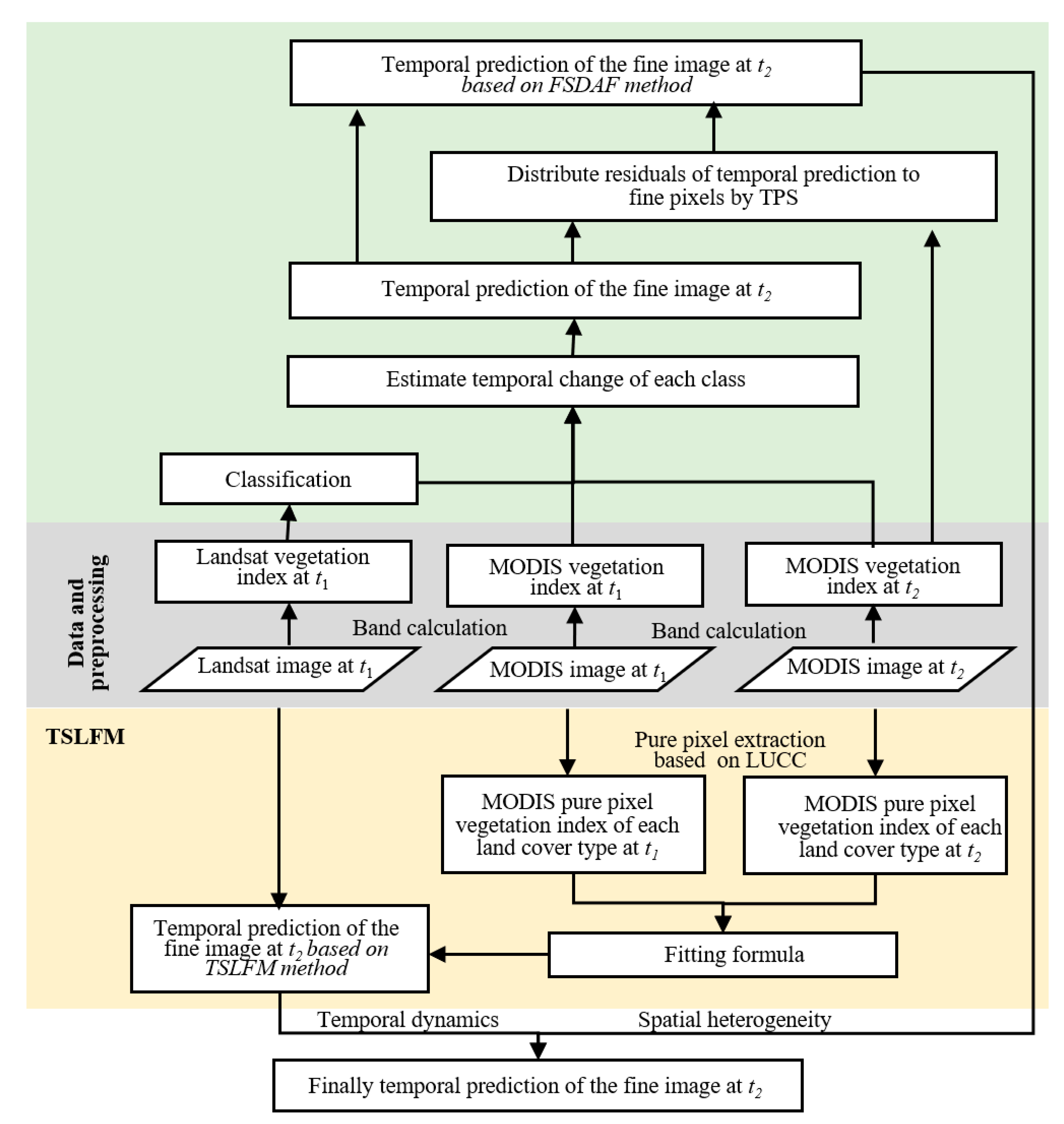
The combination of the FSDAF method [22] and the time series linear fitting model (TSLFM method) [19,48] enabled the fusing of Landsat and MODIS datasets. The FSDAF technique produces fused images that exhibited higher accuracy and preserved more detailed spatial information, especially in land use and cover change regions, than alternative fusion methods [22]. The TSLFM method was effective at capturing the temporal dynamics inherent in the MODIS dataset [19,48]. Firstly, we individually utilized the FSDAF and TSLFM methods to calculate high-spatial resolution images for the YRD from 2000 to 2020. Subsequently, we employed the time series characteristics of the images obtained through the TSLFM method, as well as the spatial heterogeneity attributes acquired through the FSDAF method, to generate the final fused vegetation index (Figure 2).
Within the framework of the spatiotemporal data fusion method, the input data consisted of a set of images, namely a pair of coarse-(MODIS) and fine-resolution (Landsat) images acquired at time t1, in addition to a single coarse-resolution image obtained at time t2. The output data were predicted as fine-resolution images at time t2, which were characterized by an enhanced spatiotemporal resolution, featuring a spatial resolution of 30 × 30 m and a temporal resolution of 8 days. The imaging schedules of MODIS and Landsat were not concurrent. Given that we adopted Landsat data at time t1 as the baseline, we opted for the nearest available MODIS image, in terms of acquisition date, to serve as the coarse-resolution dataset for time t1. Furthermore, it was essential that the acquisition times of fine- and coarse-resolution images at t1 and t2 should be the differences. For the time t1, a preference was accorded to the selection of images captured during the active growth season and the period of peak vegetation. However, for time t2, non-growing season data were typically chosen. In this study, all available MOD09A1 data from 2000 to 2020 were used, along with 45 Landsat images with minimal or no cloud cover (Table 1), which were used as the reference data. Notably, this configuration of input data was critical to the success of the FSDAF technique, as it enabled the algorithm to leverage the spatial and temporal information present in the input data.

2.3.1. FSDAF Method

The FSDAF methodology encompassed six key steps to effectively fuse remote sensing data [22]. Here, we briefly outline the principal processes and relevant equations as follows:
(1)
Classification of fine-resolution image
The initial step involved categorizing the fine-resolution image taken at time t1 to assign distinct land cover classes. An unsupervised classifier was adopted for this purpose.
(2)
Temporal dynamics estimation
The temporal dynamics for each land cover class within the coarse-resolution image from t1 to t2 were estimated. The temporal alteration of a coarse pixel was computed as a weighted summation of the temporal changes across all classes within it, as expressed by the following equation:
Δ C ( x i , y i , b ) = c = 1 l f c ( x i , y i ) × Δ F ( c , b ) ,
where (xi, yi) represents the coordinate index of the ith pixel, ΔC(xi, yi, b) represents the change in the band value of the (xi, yi) coarse pixel between t1 and t2, ΔF(c, b) represent the change in the band b value of class c at fine resolution between t1 and t2, fc(xi, yi) represents the proportion of class c of the (xi, yi) coarse pixel, and i represents the index of a coarse pixel;
(3)
Prediction of fine-resolution image
By leveraging class-level temporal changes, the fine-resolution image at t2 was predicted, and residuals were calculated at each coarse pixel. This prediction relied solely on the temporal change information, omitting any spatial considerations. The prediction equation was formulated as follows:
F 2 T P ( x i j , y i j , b ) = F 1 ( x i j , y i j , b ) + Δ F ( c , b ) ,
where F 2 T P ( x i j , y i j , b ) represents the temporal prediction, and j represents the index of a fine pixel within one coarse pixel, i.e., j = 1,…, m;
R ( x i , y i , b ) = Δ C ( x i , y i , b ) 1 m [ j = 1 m F 2 T P ( x i j , y i j , b ) j = 1 m F 1 ( x i j , y i j , b ) ] ,
where R ( x i , y i , b ) represents the distribution residual of fine pixels within a coarse pixel.
(4)
Identify TPS interpolation to guide residual distribution
TPS serves as a spatial interpolation technique used to identify point data rooted in spatial dependence [49]. The TPS interpolator was employed to distinguish between the fine-resolution image and the coarse-resolution image at t2. The TPS equation is represented as follows:
f T P S b ( x , y ) = a 0 + a 1 x + a 2 y + 1 2 i = 1 N b i r i 2 l o g r i 2 ,
where f T P S b ( x , y ) represents the basic TPS function for band b of N known points. The prediction of fine pixels is expressed as follows:
F 2 S P ( x i j , y i j , b ) = f T P S b ( x i j , y i j ) ,
(5)
Distribute residuals to fine pixels
The distribution of the residuals from the temporal prediction to individual fine pixels inside of each coarse pixel is the key step required to improve the accuracy of the temporal prediction.
Δ F ( x i j , y i j , b ) = m × R ( x i , y i , b ) × W ( x i j , y i j , b ) + Δ F ( c , b ) ,
where Δ F ( x i j , y i j , b ) represents the prediction of the total change in a fine pixel between t1 and t2, and W ( x i j , y i j , b ) represents the weight.
(6)
Robust prediction of fine image using neighborhood
The robust prediction of the fine image is derived by considering neighboring information. The essential equations for this process are as follows:
F 2 , F S D A F ( x i j , y i j , b ) = F 1 ( x i j , y i j , b ) + k 1 n w k × Δ F ( x k , y k , b ) ,
w k = ( 1 / D k ) / k 1 n ( 1 / D k ) ,
D k = 1 + ( x k x i j ) 2 + ( y k y i j ) 2 / ( w / 2 )   ,
Δ F ( x i j , y i j , b ) = r ( x i j , y i j , b ) + Δ F ( c , b ) ,
where F 2 ^ ( x i j , y i j , b ) is the temporal prediction of the fine image at t2 based on the FSDAF method; Dk is a relative distance ranging from −1 to 1, and w is the size of the neighborhood (for more details, see Zhu et al. (2016) [22]).

2.3.2. TSLFM Method

The input data of the TSLFM method consisted of a set of MODIS and Landsat images at time t1, along with a Landsat image at time t2, which were similar to those of the FSDAF method. The output data were predicted as fine-resolution images at time t2. The FSDAF methodology encompassed three key steps that effectively fused remote sensing data Here, we briefly outline the principal processes and relevant equations:
(1)
Extraction of pure pixels
The land cover data were resampled to exactly match the rows and columns of the Landsat data. Then, based on the resampled land over data, each coarse-resolution pixel was examined to determine whether it represented a pure pixel. If the land cover type within the range of a coarse-resolution pixel was entirely consistent, the pixel was considered to be a pure pixel.
(2)
Construction of correlation function
We used formulated fitting equations to determine the average vegetation indices of pure pixels of different vegetation types at times t1 and t2.
C 2 ¯ ( l , b ) = m × C 1 ¯ ( l , b ) + n ,
where m and n denote fitting parameters, l denotes various vegetation types, and C 1 ¯ and C 2 ¯ denote the average vegetation indices of pure pixels of vegetation type l at times t1 and t2, respectively.
(3)
Prediction of fine image
Based on the fine pixel data at time t1 and using the fitting parameters m and n, we calculated the values of fine pixels for different vegetation types at time t2:
F 2 , T S L F M ( l , b ) = m × F 1 ( l , b ) + n ,
where F1 and F2 represent the fine-resolution b band at times t1 and t2, respectively.

2.3.3. Integration of Simulation Results of FSDAF and TSLFM Methods

Finally, we integrated the temporal variation trends from the TSLFM simulation results into the spatial heterogeneity information derived from the FSDAF simulation results to generate the fused vegetation index data.
F 2 , F u s e d ( l , b ) = F 2 , T S L F M ( l , b ) ¯ + Δ F 2 , F S D A F ( l , b ) ,
Δ F 2 , F S D A F ( l , b ) = F 2 , F S D A F ( l , b ) F 2 , F S D A F ( l , b ) ¯ ,
where F 2 , F u s e d represents the finally fused fine-resolution image data, F 2 , T S L F M ( l , b ) ¯ represents the average value of the b band simulated via the TSLFM method at time t2, and F 2 , F S D A F ( l , b ) ¯ represents the average value of the b band simulated via the FSDAF method at time t2.

2.4. Statistical Analysis

A piecewise linear regression (PLR) model [50,51] was employed to identify potential EVI trends from 2000 to 2020. The PLR method is a well-known technique used to detecti turning points in time-series data:
y = { β 0 + β 1 t + ε t         t α β 0 + β 1 t + β 2 ( t α ) + ε t         t > α ,
where t is year in annual EVI; α is the visually estimated turning point of the time series defining the timing of a trend change; β0, β1, and β2 are regression coefficients, with the three regression coefficients being determined using the least squares linear regression; and ε is the residual of the fit. A p value of less than 0.05 was considered to be significant.
The analysis of EVI trends was conducted using the linear least squares regression method, allowing us to assess the slope of EVI changes at both the regional and pixel scales. The determination coefficient (R2) was employed to assess the impact of various factors on the EVI trend. A p value of less than 0.05 was considered to be significant.

3. Results

3.1. Spatial Pattern of Vegetation Variations

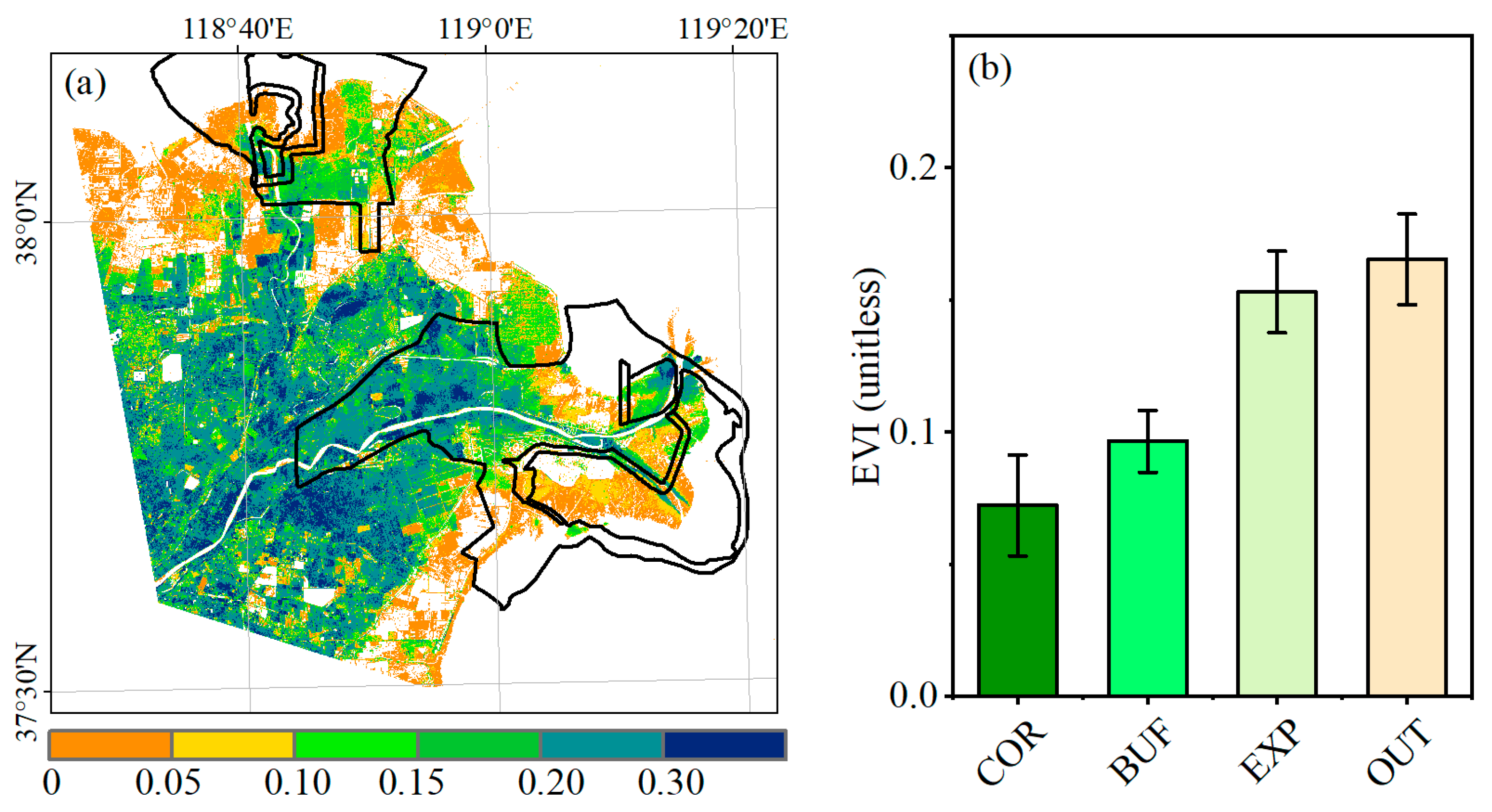
The annual average fused EVI in the YRD in 2020 is illustrated in Figure 3. The regions along the banks of the Yellow River exhibited the highest EVI values, typically exceeding 0.20, while the coastal regions displayed the lowest EVI values, which were below 0.10 (Figure 3a). In the protected areas, the EVI values tended to be lower than in the outside area (Figure 3b). Specifically, the core zone of the YRDNNR displayed the lowest average EVI, having a value of 0.07 ± 0.02; the buffer zone showed slightly higher EVI values, averaging approximately 0.10 ± 0.01. Notably, the experimental zone within the protected area exhibited an annual average EVI of approximately twice that of the core zone, reaching approximately 0.15 ± 0.02. Furthermore, the average EVI outside of the protected zones closely resembled that of the experimental zone, being approximately 0.17 ± 0.02 (Figure 3b).

3.2. The Temporal Trends of the Fused EVI

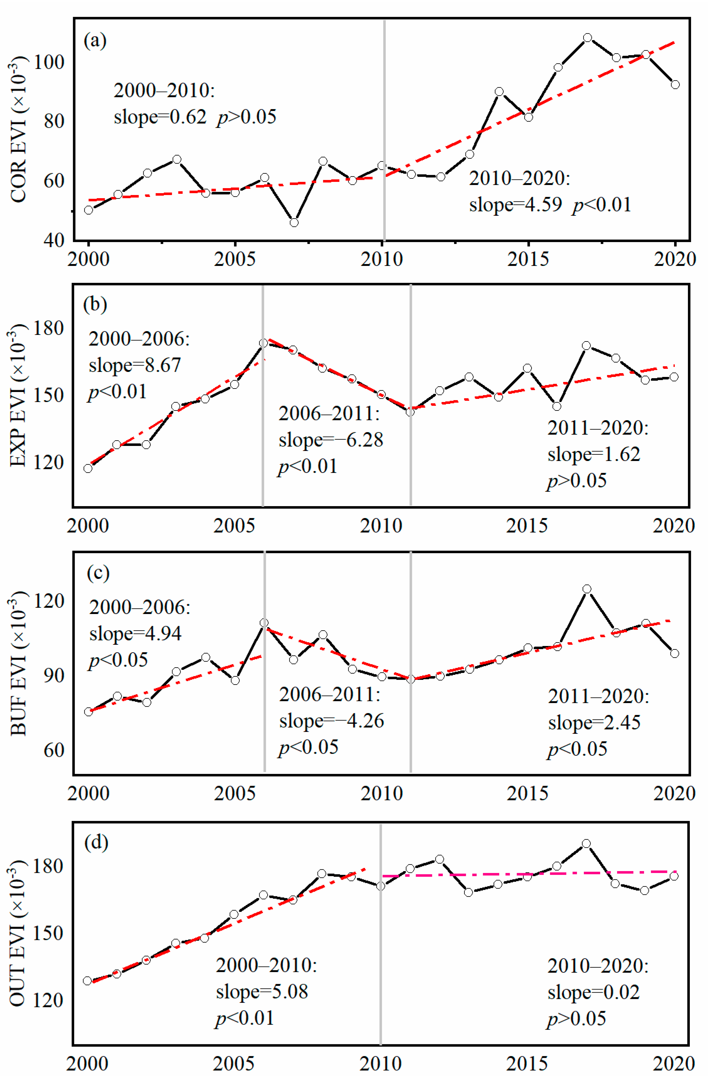
There was a remarkable improvement in the vegetation of the whole YRD from 2000 to 2020, as evidenced by a significant increase in the fused EVI. However, the trends of EVI greatly vary between the core area, buffer zone, experimental area, and area outside of the protected area in the YRDNNR. Specifically, the core area’s EVI did not exhibit significant variation before 2010, while there was a rapidly increasing trend after 2010, with an annual increase rate of 4.59 × 10⁻³ a−1 (p < 0.01), accounting for approximately 7% of the multiyear average core area’s EVI (Figure 4a). The experimental area’s EVI exhibited a fluctuating pattern characterized by an initial increase, followed by a subsequent decrease and, ultimately, a recovery with elevated values, with annual increasing rates of 8.67 × 10⁻³ a−1 (p < 0.01) from 2000 to 2006, −6.28 × 10⁻³ a−1 (p < 0.01) from 2006 to 2011, and 1.62 × 10⁻³ a−1 after 2011 (Figure 4b). The variations in the EVI of the buffer area were similar to those in the experimental area (Figure 4c). The area outside of the protected area’s EVI experienced a rapid increasing trend from 2000 to 2010, having a value of 5.08 × 10⁻³ a−1 (p < 0.01), while the trend stabilized after 2010 (Figure 4d).
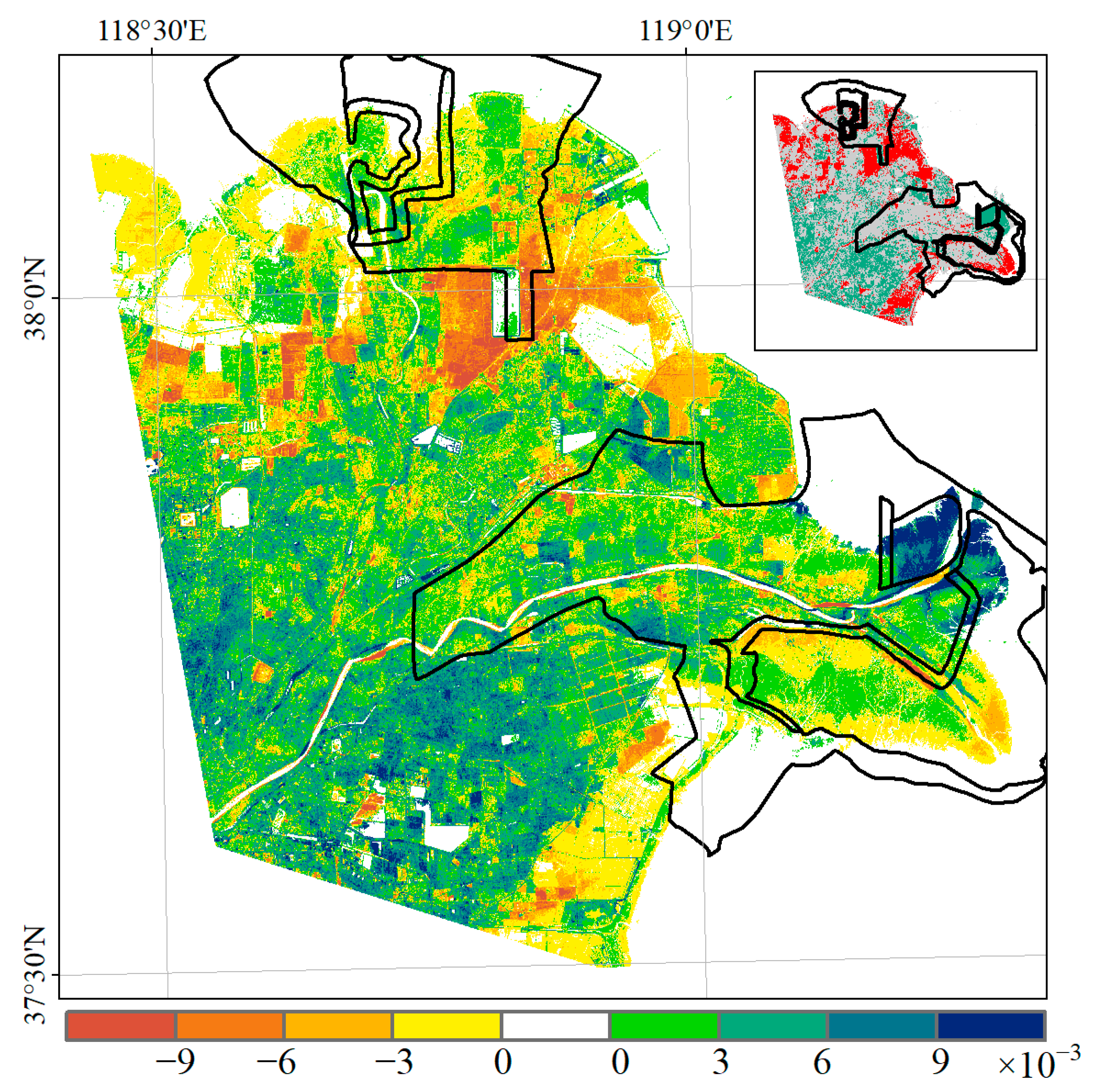
We also investigated the spatial patterns of the interannual variations in the fused EVI in the YRD from 2000 to 2020 (Figure 5). Approximately 58% of the study area showed increasing EVI trends, with 25% of the area exhibiting a significant increasing trend. The areas with significant EVI upward trends were mainly distributed in the Yellow River North Estuary and outside of the YRDNNR. Meanwhile, approximately 19% of the study area showed significant decreasing trends in the EVI; these subareas were mainly distributed in the northern part of the YRD and the eastern coastal areas.

3.3. The Driving Factors of Vegetation Variations in the YRD

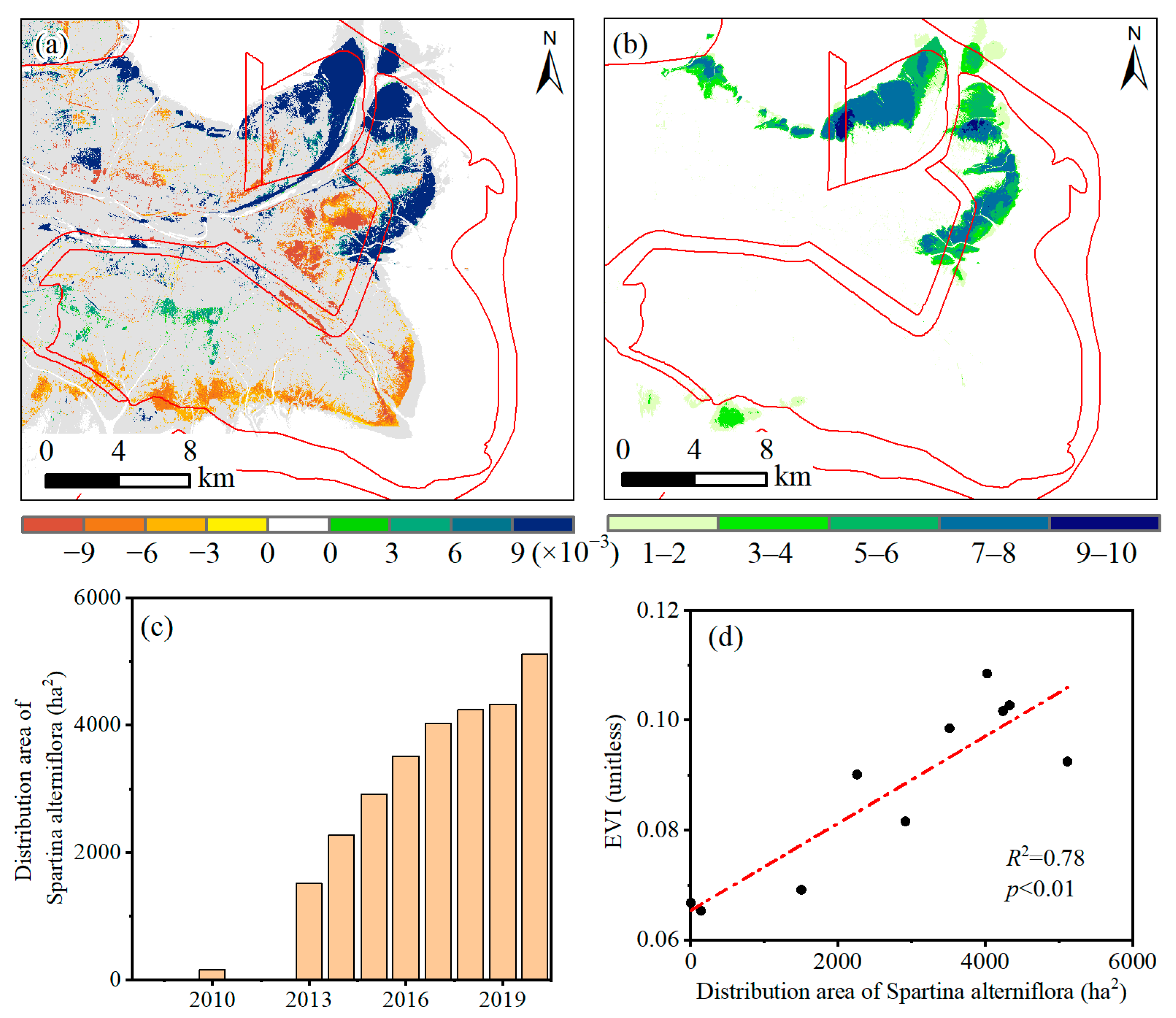
Notable differences in vegetation trends were observed across various regions of the YRD from 2000 to 2020, which were primarily attributable to several distinct driving factors. The invasion of Spartina alterniflora has been identified as the predominant driver behind the significant increasing trend in the EVI of the core area of YRDNNR since 2010. Following its initial appearance in the Yellow River Estuary in 2010, the Spartina alterniflora invasion area has expanded rapidly (Figure 6c). The distribution area of Spartina alterniflora substantially overlapped with the areas of remarkable EVI increase (Figure 6a,b), and the distribution area of Spartina alterniflora explained 78% of the fused EVI variations identified in the core zone (Figure 6d). In different seasons, regions with significant increases in EVI were also highly consistent with areas invaded by Spartina alterniflora (Figure 7).
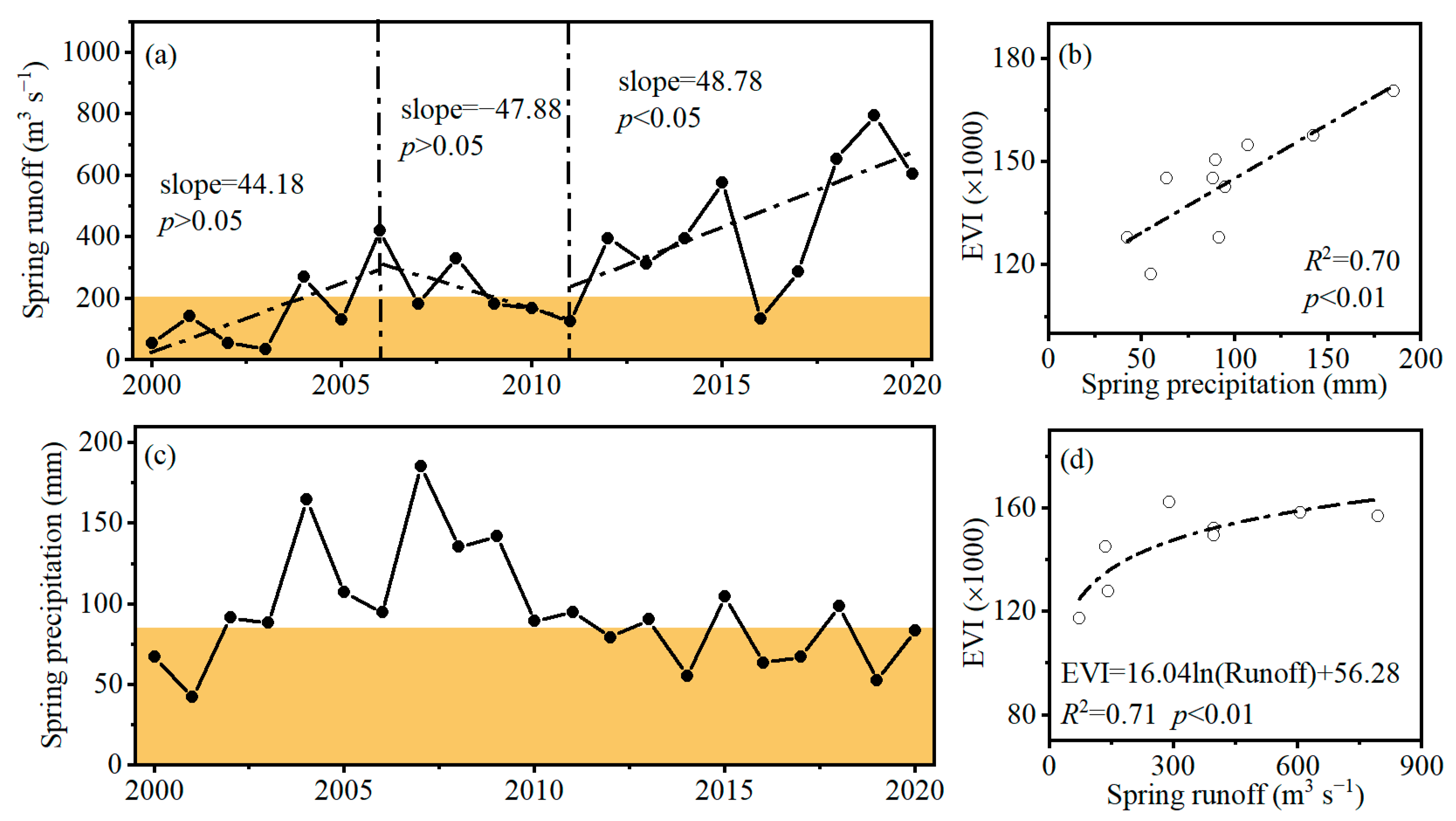
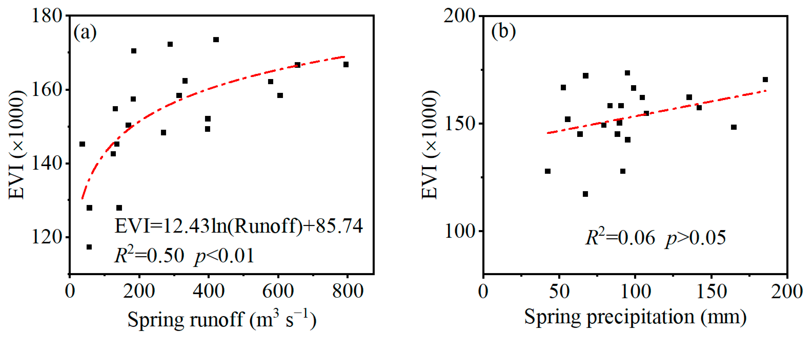
Within the experimental area of the protected zone, the temporal dynamics of the fused EVI were primarily influenced by variations in the spring runoff. Additionally, for years characterized by lower spring runoff levels, the dynamics of the fused EVI were influenced by the spring precipitation. Specifically, from 2000 to 2020, the temporal variations in the spring runoff were consistent with those in the EVI, which were characterized by an initial increase, followed by a subsequent decrease and, ultimately, a recovery with elevated values, with annual increasing rates of 44.18 m3 s−1 a−1, −47.88 m3 s−1 a−1 (p < 0.01), and 48.78 m3 s−1 a−1 recorded from 2000 to 2006, from 2006 to 2011, and after 2011 (Figure 8a). Meanwhile, the spring runoff is significantly positively correlated with the EVI of the experimental area from 2000 to 2020, recording a R2 value of 0.50 (p < 0.01) (Figure 9a). In particular, for years with relatively lower spring precipitation, such as 2000, 2001, 2012, 2014, 2016, 2017, 2019, and 2020, when the spring precipitation was below 85 mm (Figure 8c), the R2 between the spring runoff and EVI in the experimental area reached 0.71 (p < 0.01) (Figure 8d). Additionally, this study revealed that there was no statistically significant correlation (p > 0.05) between the spring precipitation and the EVI of the experimental area from 2000 to 2020 (Figure 9b); however, in years with relatively low spring runoff levels, such as 2000–2003, 2005, 2007, 2009–2011, and 2016, when the spring runoff was less than 200 m3 s−1 (Figure 8a), the experimental area’s EVI and the spring precipitation showed a significant positive relationship, recording a coefficient of determination of 0.70 (p < 0.01) (Figure 8b).
The significantly increasing trend of the EVI outside of the protected area from 2000 to 2010 was primarily driven by the expansion of farmland and the rapid increase in the EVI per unit area (Figure 10). Specifically, during this period, the farmland area rapidly expanded, having a notable increase of 31%. Meanwhile, the fused EVI per unit area of farmland increased at an average annual rate of 6.48 × 10⁻³ a−1 (p < 0.01). However, both the area of farmland and the EVI per unit area remained relatively stable after 2010, leading to the relative stability of the EVI outside of the protected area.

4. Discussion

4.1. Accuracy of the Fused Data

Generating high-quality and high-spatial–temporal resolution satellite-based data is essential when investigating vegetation variations in estuarine wetlands. The FSDAF method utilized in this study integrates the unmixing-based method and the concept of STARFM into a unified framework; meanwhile, the FSDAF method could adaptively select coarse pixels related to each endmember, which contain similar land cover types, to preserve more spatial information in the predicted high-resolution images [22]. Additionally, the TSLFM methods were employed to correct the temporal variations in the simulated results obtained via the FSDAF method. The TSLFM method utilizes linear regression techniques to accurately capture the temporal variation information of low-spatial resolution data [48]. We validated the accuracy of the fused EVI in terms of capturing the spatiotemporal variations in vegetation in the Yellow River Delta based on Landsat and MODIS data.
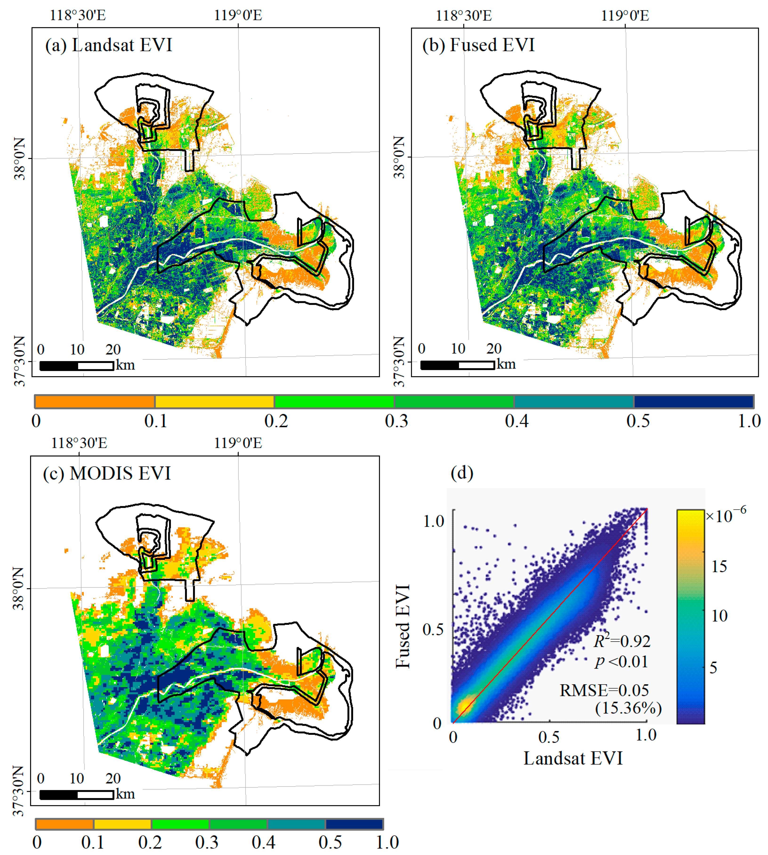
The spatial distribution patterns of Landsat, fused, and MODIS EVIs were compared in the YRD on around day 233 of 2008 (Figure 11). The spatial distribution patterns of these three datasets were remarkably similar. Specifically, the regions along the banks of the Yellow River exhibited the highest EVI values, surpassing 0.5, while the coastal regions displayed the lowest EVI values, being below 0.2. Furthermore, we investigated the relationships between Landsat and fused EVIs at the pixel scale (Figure 11d). The results showed a significant correlation between the two factors (p < 0.01), recording a coefficient of determination of 0.92 and an RMSE of 0.05. The RMSE accounted for approximately 15.36% of the mean EVI values in the whole YRD.
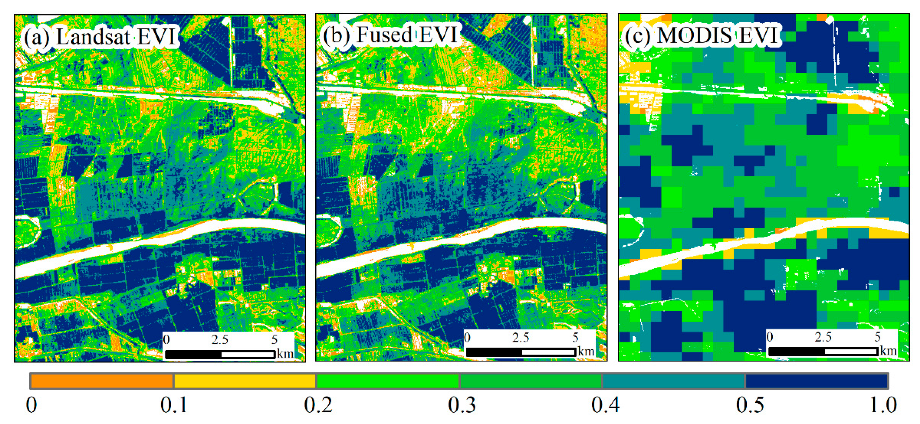
This study also compared the three datasets to evaluate their capacity to capture fine-scale vegetation spatial patterns (Figure 12). Due to the spatial resolution constraint, MODIS EVI data cannot provide sufficient detailed information to accurately reflect the spatial heterogeneity in vegetation conditions at a small scale (Figure 12c). Conversely, the fused EVI data exhibited excellent spatial details, allowing the delineation of field boundaries, roads, river distributions, and other small-scale features (Figure 12b). The spatially resolved information conveyed by the fused EVI data had strong consistency with that derived from Landsat EVI (Figure 12a), attesting to its efficacy in capturing intricate spatial nuances.
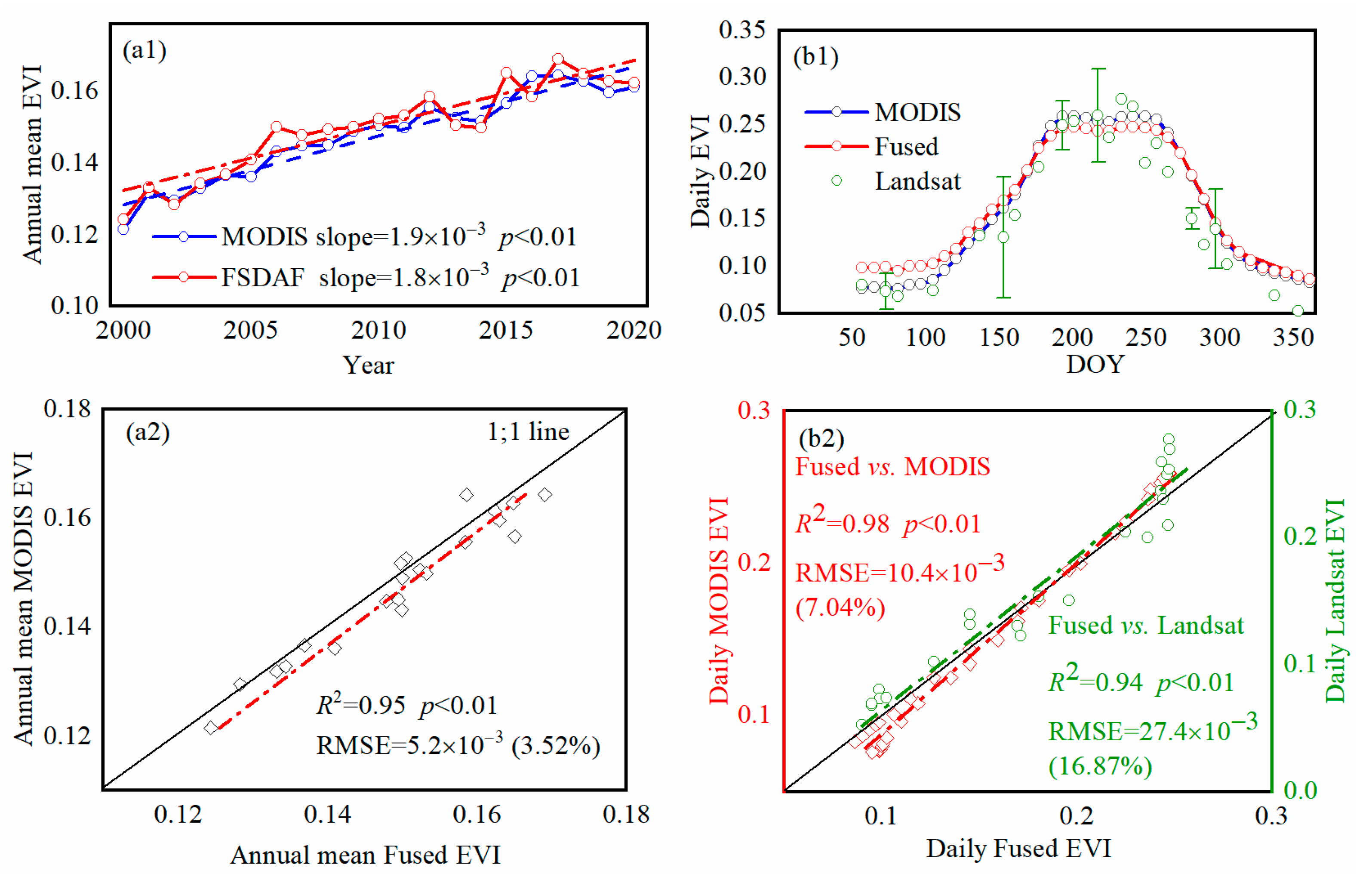
The interannual and seasonal variations between the fused EVI and MODIS EVI are compared in Figure 13. At the interannual scale, both the fused EVI and MODIS EVI exhibited a statistically significant increasing trend (p < 0.01), and the vegetation growth rates were 1.8 × 10⁻³ and 1.9 × 10⁻³, respectively, which suggested a consistent increase in vegetation productivity over time (Figure 13a1). Meanwhile, a strong and significant correlation between the two fused EVI and MODIS EVI, with a coefficient of determination of 0.95 and an RMSE of 5.2 × 10⁻³, accounted for approximately 3.52% of the average annual EVI (Figure 13a2). At the seasonal scale, the fused EVI, MODIS EVI, and Landsat EVI demonstrated unimodal patterns, which were characterized by a peak in vegetation productivity (Figure 13b1). Specifically, the highest average EVI values were observed within the period ranging from the 200th to the 260th day, with values reaching approximately 0.25. Meanwhile, the EVI values were comparatively lower, falling below 0.10 during the period ranging from 0 to 100 days. Furthermore, their daily-scale relationship indicated a strong and significant correlation, with a R2 of 0.98 and an RMSE of 10.4 × 10⁻³, accounting for approximately 7.04% of the average daily EVI (Figure 13b2). In addition, the Fused EVI and Landsat EVI exhibited a strong correlation (p < 0.01), with a R2 of 0.94 and a RMSE of 10.4 × 10⁻³. These results demonstrate that the fused dataset not only enhances the spatial representation of details in remote sensing-based vegetation monitoring, but also effectively captures the dynamics of vegetation change processes. This study demonstrated that the fused data successfully captured the vegetation variations in the YRD, which supports past vegetation dynamic studies of estuarine wetlands.

4.2. Driving Factors of Vegetation Dynamics

The estuarine wetlands of the YRD exhibited an overall increasing trend in the EVI, and the dominant factors significantly varied across different regions. For the core area of the YRDNNR, the increasing EVI was primarily driven by the invasion of Spartina alterniflora. Spartina alterniflora, originating from North America, is widely regarded as one of the most detrimental invasive species in several regions [52]. The invasion of Spartina alterniflora in the YRD may date to 1989, when it was initially brought from Fujin Province with the aim of protecting the fragile and muddy coast from erosion caused by tides and ocean currents [53]. Spartina alterniflora predominantly thrives in the lower intertidal zone, colonizing areas in which most local plant communities cannot survive [54,55]. After a prolonged latency period, the invasive range of Spartina alterniflora exhibited rapid expansion after 2010 [39,40]. Data provided by the Lijin Hydrological Station (the nearest hydrological station to the YRD) indicate that in 2010 and 2013, the Yellow River underwent water and sediment diversion activities, which led to a significant deposition of sediment in the Yellow River Delta, resulting in a substantial increase in the area of the Spartina alterniflora community on the northern bank of the Yellow River estuary [31]. The expansion resulted in a significant increase in the EVI within the invaded areas and positively contributed to coastal protection. However, it also resulted in significant degradation of the local ecosystem and brought forth a multitude of adverse effects [56].
The interplay between the spring runoff and the spring precipitation played a crucial role in shaping the vegetation trends within the experimental area. The vegetation in the YRD is strongly influenced by groundwater depth and salinity gradients [57,58]. Freshwater inflow has a significant impact on water and salt regulation, thereby affecting plant communities and vegetation dynamics [59,60]. Previous studies have indicated that vegetation NDVI in the YRD is higher in areas closer to the river channel [36]. In years in which the spring runoff was abundant, it acted as the main driving force behind the variations in fused EVI, with higher runoff levels generally correlating with increased vegetation productivity. Spring is characterized by relatively low precipitation, accounting for only 15% of the total annual precipitation, making runoff an important water source for vegetation growth, especially when precipitation is scarce. In years with less pronounced spring runoff, the influence of the spring precipitation became more pronounced, and the vegetation response showed a strong positive correlation with the amount of precipitation during this period. These findings highlight the complexity of vegetation dynamics within the protected zone and underscore the significance of both the spring runoff and the spring precipitation as key determinants of vegetation productivity. Understanding the interactive effects of these hydrological factors can contribute to the performance of more accurate and comprehensive assessments of ecosystem dynamics in the study area.
Human activities dominated the vegetation changes outside of the YRDNNR. In recent years, the YRD has experienced a substantial increase in human activities and the expansion of artificial landscapes, and anthropogenic influence has emerged as a primary driver of ecosystem transformations [15]. Notably, during the 2000s, there was a rapid expansion of agricultural land in the YRD, which was facilitated via effective irrigation management, resulting in a notable increase in the maximum vegetation index during the growing season [36]. In November 2009, the State Council of the People’s Republic of China approved the “Development Plan for a High-Efficiency Ecological and Economic Zone in the Yellow River Delta,” highlighting the pivotal significance of ecological construction and environmental protection. This development led to a diminishing trend in the expansion of agricultural land, eventually resulting in the reduction in the total farmland area. Meanwhile, the hydrological connectivity in the YRD had a gradually increased in recent years [61]. Human activities play a significant role in influencing the vegetation dynamics changes in the Yellow River Delta.
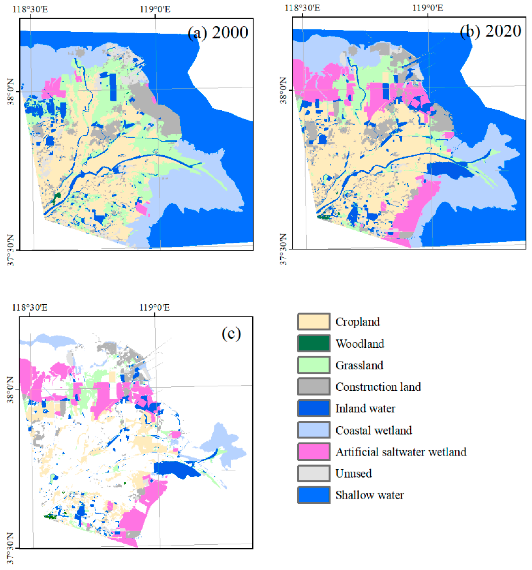
Additionally, a considerable conversion of natural wetlands and grasslands located outside of the reserve into artificial wetlands has led to a significant decline in the vegetation index in coastal regions (Figure 14).
There were also limitations in this study, such as the absence of on-site data validation and an insufficient understanding of driving factors. In further studies, we will conduct field data sampling to determine changes in vegetation biomass and productivity. Simultaneously, we will integrate factors like soil salinity and hydrological connectivity to delve deeper into the mechanisms driving the vegetation dynamics.

5. Conclusions

This study integrated the FSDAF and TSLFM methods to construct a novel fused EVI dataset with a high spatiotemporal resolution and analyzed the variations in the vegetation dynamics and their driving factors within and outside of the YRDNRR from 2000 to 2020. The main conclusions were as follows:
(1)
In the core area of the YRDNRR, the fused EVI did not exhibit a significant trend before 2010, while a notable increasing trend was observed after 2010, with an annual increase of 7%; the invasion of Spartina alterniflora was identified as the primary driving factor, explaining 78% of the EVI increment.
(2)
In the experimental area of YRDNRR, the fused EVI showed a distinct interannual trend characterized by an initial increase (2000–2006, p < 0.01), followed by a subsequent decrease (2006–2011, p < 0.01) and, ultimately, a renewed increase (2011–2020, p > 0.05); the dynamics of fused EVI were mainly affected by the spring runoff (R2 = 0.71), while in years with lower runoff, they was also affected by the spring precipitation (R2 = 0.70).
(3)
Outside of the protected area, the fused EVI demonstrated a substantial increase from 2000 to 2010 due to the expansion of agricultural land and human management practices, followed by stabilization after 2010.
This study has not only enhanced our understanding of the complex vegetation dynamics in the YRD, but also has implications for vegetation dynamics research in estuarine wetlands worldwide.

Author Contributions

Conceptualization, Z.N., B.S. (Bingcheng Si) and B.W.; Formal analysis, Z.N.; Funding acquisition, Z.N.; Methodology, Z.N.; Resources, D.L., X.H., L.L., X.L. and Z.M.; Software, Z.N. and L.L.; Supervision, B.W.; Validation, B.W.; Writing—original draft, Z.N.; Writing—review and editing, B.S. (Bingcheng Si), D.L., Y.Z., X.H., B.S. (Bing Song), M.Z., N.Z., X.Z. and Y.L. All authors have read and agreed to the published version of the manuscript.

Funding

This research was funded by the Natural Science Foundation of Shandong Province (grant number ZR2022QD118) and the National Natural Science Foundation of China (grant numbers 42201312 and 32271678).

Data Availability Statement

The MOD09A1 product was downloaded from https://ladsweb.modaps.eosdis.nasa.gov/search/, accessed on 1 January 2022; the Landsat data were downloaded from https://www.gscloud.cn/, accessed on 1 January 2022; the meteorological data were downloaded from http://poles.tpdc.ac.cn/en/, accessed on 1 July 2022,; the data of Spartina alterniflora were downloaded from https://geodoi.ac.cn/WebCn/doi.aspx?Id=1989, accessed on 1 May 2023; the runoff data were downloaded from http://www.yrcc.gov.cn/, accessed on 1 January 2022.

Conflicts of Interest

The authors declare no conflict of interest.

References

  1. Li, S.; Xie, T.; Bai, J.; Cui, B. Degradation and Ecological Restoration of Estuarine Wetlands in China. Wetlands 2022, 42, 90. [Google Scholar] [CrossRef]
  2. Wang, X.; Xiao, X.; Xu, X.; Zou, Z.; Chen, B.; Qin, Y.; Zhang, X.; Dong, J.; Liu, D.; Pan, L. Rebound in China’s coastal wetlands following conservation and restoration. Nat. Sustain. 2021, 4, 1076–1083. [Google Scholar] [CrossRef]
  3. Zhou, Y.; Tian, B.; Huang, Y.; Wu, W.; Qi, X.; Shu, M.; Xu, W.; Ge, F.; Wei, W.; Huang, G. Degradation of coastal wetland ecosystem in China: Drivers, impacts, and strategies. Bull. Chin. Acad. Sci. 2016, 31, 1157–1166. [Google Scholar]
  4. Hou, X.; Liu, J.; Song, Y.; Li, X. Environmental-ecological effect of development and utilization of China’s coastline and policy recommendations. Bull. Chin. Acad. Sci. 2021, 31, 1143–1150. [Google Scholar]
  5. Osland, M.J.; Chivoiu, B.; Enwright, N.M.; Thorne, K.M.; Guntenspergen, G.R.; Grace, J.B.; Dale, L.L.; Brooks, W.; Herold, N.; Day, J.W. Migration and transformation of coastal wetlands in response to rising seas. Sci. Adv. 2022, 8, eabo5174. [Google Scholar] [CrossRef]
  6. Guangxuan, H.; Weimin, S.; Peiguang, L.; Xiaojie, W.; Guangmei, W.; Xiaojing, C. Long-term ecological research support protection of coastal wetland ecosystems. Bull. Chin. Acad. Sci. (Chin. Version) 2020, 35, 218–228. [Google Scholar]
  7. Niu, B.; Zhang, Z.; Yu, X.; Li, X.; Wang, Z.; Loáiciga, H.A.; Peng, S. Regime shift of the hydroclimate–vegetation system in the Yellow River Delta of China from 1982 through 2015. Environ. Res. Lett. 2020, 15, 024017. [Google Scholar] [CrossRef]
  8. Gao, Y.; Song, X.; Li, W.; Wang, J.; He, J.; Jiang, X.; Feng, Y. Fusion classification of HSI and MSI using a spatial-spectral vision transformer for wetland biodiversity estimation. Remote Sens. 2022, 14, 850. [Google Scholar] [CrossRef]
  9. Du, P.; Hou, X.; Xu, H. Dynamic Expansion of Urban Land in China’s Coastal Zone since 2000. Remote Sens. 2022, 14, 916. [Google Scholar] [CrossRef]
  10. Su, H.; Yao, W.; Wu, Z.; Zheng, P.; Du, Q. Kernel low-rank representation with elastic net for China coastal wetland land cover classification using GF-5 hyperspectral imagery. ISPRS J. Photogramm. Remote Sens. 2021, 171, 238–252. [Google Scholar] [CrossRef]
  11. Tang, Y.-N.; Ma, J.; Xu, J.-X.; Wu, W.-B.; Wang, Y.-C.; Guo, H.-Q. Assessing the Impacts of Tidal Creeks on the Spatial Patterns of Coastal Salt Marsh Vegetation and Its Aboveground Biomass. Remote Sens. 2022, 14, 1839. [Google Scholar] [CrossRef]
  12. Yu, L.; Zhuang, T.; Bai, J.; Wang, J.; Yu, Z.; Wang, X.; Zhang, G. Effects of water and salinity on soil labile organic carbon in estuarine wetlands of the Yellow River Delta, China. Ecohydrol. Hydrobiol. 2020, 20, 556–569. [Google Scholar] [CrossRef]
  13. LaFond-Hudson, S.; Sulman, B. Modeling strategies and data needs for representing coastal wetland vegetation in land surface models. New Phytol. 2023, 238, 938–951. [Google Scholar] [CrossRef] [PubMed]
  14. Woltz, V.L.; Stagg, C.L.; Byrd, K.B.; Windham-Myers, L.; Rovai, A.S.; Zhu, Z. Above-and Belowground Biomass Carbon Stock and Net Primary Productivity Maps for Tidal Herbaceous Marshes of the United States. Remote Sens. 2023, 15, 1697. [Google Scholar] [CrossRef]
  15. Chi, Y.; Shi, H.; Zheng, W.; Sun, J.; Fu, Z. Spatiotemporal characteristics and ecological effects of the human interference index of the Yellow River Delta in the last 30 years. Ecol. Indic. 2018, 89, 880–892. [Google Scholar] [CrossRef]
  16. Cong, P.; Chen, K.; Qu, L.; Han, J. Dynamic changes in the wetland landscape pattern of the Yellow River Delta from 1976 to 2016 based on satellite data. Chin. Geogr. Sci. 2019, 29, 372–381. [Google Scholar] [CrossRef]
  17. Lu, G.; Han, M.; Xu, Z.-H.; Zhu, J.-Q.; Niu, X.-R. Spatiotemporal variations of net primary productivity in new wetlands of the Yellow River Delta. Chin. J. Ecol. 2019, 38, 1113. [Google Scholar]
  18. Gao, F.; Masek, J.; Schwaller, M.; Hall, F. On the blending of the Landsat and MODIS surface reflectance: Predicting daily Landsat surface reflectance. IEEE Trans. Geosci. Remote Sens. 2006, 44, 2207–2218. [Google Scholar]
  19. Luo, L.; Yan, H.; Niu, Z. Comparative Analysis on Three Multi-Source Remote Sensing Data Fusion Models in Monitoring Farmland Productivity. J. Geo-Inf. Sci. 2018, 20, 268–279. [Google Scholar]
  20. Gevaert, C.M.; García-Haro, F.J. A comparison of STARFM and an unmixing-based algorithm for Landsat and MODIS data fusion. Remote Sens. Environ. 2015, 156, 34–44. [Google Scholar] [CrossRef]
  21. Zhu, X.; Chen, J.; Gao, F.; Chen, X.; Masek, J.G. An enhanced spatial and temporal adaptive reflectance fusion model for complex heterogeneous regions. Remote Sens. Environ. 2010, 114, 2610–2623. [Google Scholar] [CrossRef]
  22. Zhu, X.; Helmer, E.H.; Gao, F.; Liu, D.; Chen, J.; Lefsky, M.A. A flexible spatiotemporal method for fusing satellite images with different resolutions. Remote Sens. Environ. 2016, 172, 165–177. [Google Scholar] [CrossRef]
  23. Liu, M.; Yang, W.; Zhu, X.; Chen, J.; Chen, X.; Yang, L.; Helmer, E.H. An Improved Flexible Spatiotemporal DAta Fusion (IFSDAF) method for producing high spatiotemporal resolution normalized difference vegetation index time series. Remote Sens. Environ. 2019, 227, 74–89. [Google Scholar] [CrossRef]
  24. Wang, Q.; Atkinson, P.M. Spatio-temporal fusion for daily Sentinel-2 images. Remote Sens. Environ. 2018, 204, 31–42. [Google Scholar] [CrossRef]
  25. Zeng, Y.; Hao, D.; Huete, A.; Dechant, B.; Berry, J.; Chen, J.M.; Joiner, J.; Frankenberg, C.; Bond-Lamberty, B.; Ryu, Y. Optical vegetation indices for monitoring terrestrial ecosystems globally. Nat. Rev. Earth Environ. 2022, 3, 477–493. [Google Scholar] [CrossRef]
  26. Song, H.; Huang, B. Spatiotemporal satellite image fusion through one-pair image learning. IEEE Trans. Geosci. Remote Sens. 2012, 51, 1883–1896. [Google Scholar] [CrossRef]
  27. Emelyanova, I.V.; McVicar, T.R.; Van Niel, T.G.; Li, L.T.; Van Dijk, A.I. Assessing the accuracy of blending Landsat–MODIS surface reflectances in two landscapes with contrasting spatial and temporal dynamics: A framework for algorithm selection. Remote Sens. Environ. 2013, 133, 193–209. [Google Scholar] [CrossRef]
  28. Shen, H.; Jiang, M.; Li, J.; Yuan, Q.; Wei, Y.; Zhang, L. Spatial–spectral fusion by combining deep learning and variational model. IEEE Trans. Geosci. Remote Sens. 2019, 57, 6169–6181. [Google Scholar] [CrossRef]
  29. Shen, H.; Meng, X.; Zhang, L. An integrated framework for the spatio–temporal–spectral fusion of remote sensing images. IEEE Trans. Geosci. Remote Sens. 2016, 54, 7135–7148. [Google Scholar] [CrossRef]
  30. Wu, J.; Lin, L.; Li, T.; Cheng, Q.; Zhang, C.; Shen, H. Fusing Landsat 8 and Sentinel-2 data for 10-m dense time-series imagery using a degradation-term constrained deep network. Int. J. Appl. Earth Obs. Geoinf. 2022, 108, 102738. [Google Scholar] [CrossRef]
  31. Gong, Z.; Zhang, C.; Zhang, L.; Bai, J.; Zhou, D. Assessing spatiotemporal characteristics of native and invasive species with multi-temporal remote sensing images in the Yellow River Delta, China. Land Degrad. Dev. 2021, 32, 1338–1352. [Google Scholar] [CrossRef]
  32. Zhu, W.; Han, M.; Kong, X.; Li, Y.; Kong, F.; Wei, F.; Rong, J. Spatiotemporal characteristics of human activity intensity and its driving factors in the Yellow River Delta from 1990 to 2018. Res. Soil Water Conserv. 2021, 28, 287–292. [Google Scholar]
  33. Zhu, W.; Muhammad, A.; Han, M.; Li, Y.; Kong, X.; Kong, F. Spatial distribution and aggregation of human-environment coordination and optimal paths in the Yellow River Delta, China. Ecol. Indic. 2022, 143, 109380. [Google Scholar] [CrossRef]
  34. Jia, G.; Hu, W.; Zhang, B.; Li, G.; Shen, S.; Gao, Z.; Li, Y. Assessing impacts of the Ecological Retreat project on water conservation in the Yellow River Basin. Sci. Total Environ. 2022, 828, 154483. [Google Scholar] [CrossRef]
  35. Ren, L.; Li, Y.; Yu, M.; Yang, J.; Zhan, C.; Zhou, D. Evolution of artificial wetlands in the Yellow River Delta and related driving factors during 1984-2015. J. Agric. Resour. Environ. 2020, 37, 493–502. [Google Scholar]
  36. Jiang, D.; Fu, X.; Wang, K. Vegetation dynamics and their response to freshwater inflow and climate variables in the Yellow River Delta, China. Quat. Int. 2013, 304, 75–84. [Google Scholar] [CrossRef]
  37. Dou, X.; Guo, H.; Zhang, L.; Liang, D.; Zhu, Q.; Liu, X.; Zhou, H.; Lv, Z.; Liu, Y.; Gou, Y. Dynamic Changes of the Yellow River Delta Wetland and the Influence of Human Activities. Sci. Total Environ. 2023, 899, 166239. [Google Scholar] [CrossRef] [PubMed]
  38. Gao, R.; Zhiyong, W.; Xiaodong, Z.; Liu, R. Monitoring and analysis of wetland change dynamics in the Yellow River Delta using multi-temporal remote sensing. Bull. Surv. Mapp. 2021, 4, 22–27. [Google Scholar]
  39. Ren, G.; Liu, Y.; Ma, Y.; Zhang, J. Spartina alterniflora monitoring and change analysis in Yellow River Delta by remote sensing technology. Acta Laser Biol. Sin 2014, 23, 596–603. [Google Scholar]
  40. Yang, J.; Ma, Y.; Ren, G.; Zhang, J.; Fan, Y. Monitoring method of invasive vegetation Spartina alterniflora in modern Yellow River delta based on gf remote sensing data. Mar. Environ. Sci. 2017, 36, 596–602. [Google Scholar]
  41. Wei, C.; Guo, B.; Lu, M.; Zang, W.; Yang, F.; Liu, C.; Wang, B.; Huang, X.; Liu, Y.; Yu, Y. The Changes in Dominant Driving Factors in the Evolution Process of Wetland in the Yellow River Delta during 2015–2022. Remote Sens. 2023, 15, 2858. [Google Scholar] [CrossRef]
  42. Chen, X.; Zhang, M.; Zhang, W. Landscape pattern changes and its drivers inferred from salt marsh plant variations in the coastal wetlands of the Liao River Estuary, China. Ecol. Indic. 2022, 145, 109719. [Google Scholar] [CrossRef]
  43. Deng, S.; Chen, J.; Du, H. ENVI Remote Sensing Image Processing Method; Higher Education Press: Beijing, China, 2014. [Google Scholar]
  44. Peng, S. 1-km Monthly Precipitation Dataset for China (1901–2020); National Tibetan Plateau Data Center: Beijing, China, 2020. [Google Scholar]
  45. Peng, S. 1-km Monthly Mean Temperature Dataset for China (1901–2017); National Tibetan Plateau Data Center: Beijing, China, 2019. [Google Scholar]
  46. Hu, J.; Gong, Z.; Zhang, C.; Qiu, H. Development of a Dataset of the Spatiotemporal Distribution of Typical Salt Marsh Vegetation in the Yellow River Delta (1999–2020). J. Glob. Change Data Discov. 2022, 5, 217–224. [Google Scholar] [CrossRef]
  47. Hou, X.; Di, X.; Hou, W.; Wu, L.; Liu, J.; Wang, J.; Su, H.; Lu, X.; Ying, L.; Yu, X.; et al. Accuracy Evaluation of Land Use Mapping Using Remote Sensing Techniques in Coastal Zone of China. J. Geo-Inf. Sci. 2018, 20, 1478–1488. [Google Scholar]
  48. Yan, H.; Du, W.; Zhou, Y.; Luo, L.; Niu, Z.E. Satellite-based evidences to improve cropland productivity on the high-standard farmland project regions in Henan Province, China. Remote Sens. 2022, 14, 1724. [Google Scholar] [CrossRef]
  49. Dubrule, O. Comparing splines and kriging. Comput. Geosci. 1984, 10, 327–338. [Google Scholar] [CrossRef]
  50. Liang, W.; Yang, Y.; Fan, D.; Guan, H.; Zhang, T.; Long, D.; Zhou, Y.; Bai, D. Analysis of spatial and temporal patterns of net primary production and their climate controls in China from 1982 to 2010. Agric. For. Meteorol. 2015, 204, 22–36. [Google Scholar] [CrossRef]
  51. Toms, J.D.; Lesperance, M.L. Piecewise regression: A tool for identifying ecological thresholds. Ecology 2003, 84, 2034–2041. [Google Scholar] [CrossRef]
  52. Curnutt, J.L. Host-area specific climatic-matching: Similarity breeds exotics. Biol. Conserv. 2000, 94, 341–351. [Google Scholar] [CrossRef]
  53. Shi, D.; Tian, J.; Chen, Y. Biological and ecological characteristics of an invasive alien species Spartina in Yellow River Delta. J. Binzhou Univ. 2009, 25, 27–32. [Google Scholar]
  54. McFarlin, C.R.; Bishop, T.D.; Hester, M.W.; Alber, M. Context-dependent effects of the loss of Spartina alterniflora on salt marsh invertebrate communities. Estuar. Coast. Shelf Sci. 2015, 163, 218–230. [Google Scholar] [CrossRef]
  55. Zhu, X.; Meng, L.; Zhang, Y.; Weng, Q.; Morris, J. Tidal and meteorological influences on the growth of invasive Spartina alterniflora: Evidence from UAV remote sensing. Remote Sens. 2019, 11, 1208. [Google Scholar] [CrossRef]
  56. Ren, G.; Zhao, Y.; Wang, J.; Wu, P.; Ma, Y. Ecological effects analysis of Spartina alterniflora invasion within Yellow River delta using long time series remote sensing imagery. Estuar. Coast. Shelf Sci. 2021, 249, 107111. [Google Scholar] [CrossRef]
  57. Wu, D.; Liu, J.; Wang, W.; Ding, W.; Wang, R. Mutiscale analysis of vegetation index and topographic variables in the Yellow River Delta of China. J. Plant Ecol. (Chin. Version) 2009, 33, 237–245. [Google Scholar]
  58. Cui, B.; Yang, Q.; Zhang, K.; Zhao, X.; You, Z. Responses of saltcedar (Tamarix chinensis) to water table depth and soil salinity in the Yellow River Delta, China. Plant Ecol. 2010, 209, 279–290. [Google Scholar] [CrossRef]
  59. Cui, B.; Yang, Q.; Yang, Z.; Zhang, K. Evaluating the ecological performance of wetland restoration in the Yellow River Delta, China. Ecol. Eng. 2009, 35, 1090–1103. [Google Scholar] [CrossRef]
  60. Wang, X.; Lian, Y.; Huang, C.; Wang, X.; Wang, R.; Shan, K.; Pedroli, B.; van Eupen, M.; ElMahdi, A.; Ali, M. Environmental flows and its evaluation of restoration effect based on LEDESS model in Yellow River Delta wetlands. Mitig. Adapt. Strateg. Glob. Change 2012, 17, 357–367. [Google Scholar] [CrossRef]
  61. Yeling, L.; Bin, H.; Qing, W.; Jizeng, D.; Baoshan, C.; Wei, Y. Temporal and spatial evolution of hydrological connectivity in River-Lake-Swamps in high efficiency eco-economic zone at the Yellow River Delta from 1970–2015. J. Beijing Norm. Univ. (Nat. Sci.) 2021, 57, 2–11. [Google Scholar]
Figure 1. The geographic location of the Yellow River Delta: (a) the geographical position of the Yellow River Delta (YRD) in China; (b) the spatial distribution map of the Yellow River Delta National Nature Reserve (YRDNRR); (c) the vegetation distribution map of the YRD.
Remotesensing 15 04332 g001
Figure 2. Flowchart of the spatiotemporal data fusion method.
Remotesensing 15 04332 g002
Figure 3. (a) Spatial pattern of the annual average fused EVI of the YRD in 2020. (b) Mean EVI values in different regions of the YRD in 2020. COR = core area, BUF = buffer zone; EXP = experimental area; OUT = outside of the protected area.
Remotesensing 15 04332 g003
Figure 4. The interannual trends of the fused EVI in different areas of the YRD from 2000 to 2020: (a) depicts the interannual variation trend of the EVI in the core area of the protected zone; (b) depicts the interannual variation trend of the EVI in the experimental area of the protected zone; (c) depicts the interannual variation trend of the EVI in the buffer area of the protected zone; (d) depicts the interannual variation trend of the EVI outside of the protected zone. The dashed red line in the graph depicts the linear regression line, while the grey straight line depicts the interannual division.
Remotesensing 15 04332 g004
Figure 5. The interannual trends of the EVI in the YRD from 2000 to 2020. The insert map at the top right of the figure indicates the area of significant change in the EVI, red indicates a significant decreasing trend (p < 0.05), and green indicates a significant increasing trend (p < 0.05).
Remotesensing 15 04332 g005
Figure 6. The relationships between the EVIs and Spartina alterniflora distribution core areas of the YRD since 2010. (a) The spatial distribution of significant trends in the annual fused EVI from 2010 to 2020, (b) the distribution frequency of Spartina alterniflora since 2010, (c) the distribution area of Spartina alterniflora since 2010, and (d) the relationships between fused EVI and the distribution area of Spartina alterniflora since 2010.
Remotesensing 15 04332 g006
Figure 7. The spatial distribution of significant trends in the fused EVI during the (a) spring, (b) summer, (c) autumn, and (d) winter seasons from 2010 to 2020.
Remotesensing 15 04332 g007
Figure 8. (a) The interannual trends of the spring runoff in the YRD from 2000 to 2020, with a focus on years with runoff of less than 200 m3 s−1 (shaded area). (b) The correlation between the spring precipitation and the experimental area’s EVI, specifically for years with runoff of less than 200 m3 s−1. (c) The interannual trends of the spring precipitation in the YRD from 2000 to 2020, with a focus on years with precipitation of less 85 mm (shaded area). (d) The relationships between the spring runoff and the experimental area’s EVI for years with precipitation of less than 85 mm.
Remotesensing 15 04332 g008
Figure 9. The correlations (a) between the spring runoff and the experimental area’s EVI, (b) as well as between the spring precipitation and the experimental area’s EVI from 2000 to 2020.
Remotesensing 15 04332 g009
Figure 10. (a) The coverage of cropland area outside of the protected area, and (b) the interannual variations in cropland EVI outside of the protected area from 2000 to 2020.
Remotesensing 15 04332 g010
Figure 11. The spatial patterns of the annual average (a) Landsat EVI, (b) fused EVI, and (c) MODIS EVIs in the YRD in 2020. (d) shows the relationship between the Landsat EVI and the fused EVI at the pixel scale. The black lines in the figures represent the boundary of YRDNRR.
Remotesensing 15 04332 g011
Figure 12. The spatial comparison of (a) Landsat EVI, (b) fused EVI, and (c) MODIS EVI in a specific region (The Landsat data correspond to the 231st day of 2019, while the MODIS data correspond to the 233rd day of 2019. Latitude: 37°44′8.63″–37°52′53.24″; longitude: 118°52′2.29″–119°0′47.73″).
Remotesensing 15 04332 g012
Figure 13. The interannual and seasonal dynamics of the fused EVI and MODIS EVI: (a1) the interannual trends of the fused EVI and MODIS EVI in the YRD from 2000 to 2020; (a2) the relationships between the annual fused EVI and MODIS EVI in the YRD from 2000 to 2020; (b1) the seasonal variations in the fused EVI, MODIS EVI, and Landsat EVI of the multiyear average EVI; (b2) the relationships between the seasonal fused EVI and seasonal MODIS EVI, as well as between the seasonal fused EVI and seasonal Landsat EVI. The dashed lines in the graph represent the linear regression lines.
Remotesensing 15 04332 g013
Figure 14. The land use and land cover changes in the YRD from 2000 to 2020. (a,b) show the land cover and land use in 2000 and 2020, respectively. (c) indicates the newly added areas of each land use type. Furthermore, climate change played a significant role in the vegetation variations observed in the YRD. Previous research has indicated that temperature is a key driving factor for spring and autumn vegetation growth, while precipitation is an important hydrological factor affecting vegetation growth, besides the impact of runoff [7]. This study demonstrates the enormous potential of multisource remote sensing data fusion methods for the monitoring of vegetation changes in estuarine wetlands. The research methodology can be applied in global and regional estuarine wetlands, as well as areas with complex land surface coverage.
Remotesensing 15 04332 g014
Table 1. The Landsat data used in this study.
IDData SourceDataIDData SourceData
1Landsat5 TM20 February 200023Landsat5 TM27 January 2009
2Landsat5 TM11 June 200024Landsat5 TM19 May 2009
3Landsat5 TM4 December 200025Landsat5 TM4 June 2009
4Landsat5 TM30 June 200126Landsat5 TM14 January 2010
5Landsat5 TM8 January 200227Landsat5 TM7 June 2010
6Landsat5 TM21 September 200228Landsat5 TM2 February 2011
7Landsat5 TM12 February 200329Landsat5 TM22 March 2011
8Landsat5 TM7 August 200330Landsat5 TM7 June 2011
9Landsat5 TM15 February 200431Landsat8 OLI3 September 2013
10Landsat5 TM10 September 200432Landsat8 OLI25 January 2014
11Landsat5 TM28 October 200433Landsat8 OLI14 March 2014
12Landsat5 TM16 January 200534Landsat8 OLI12 January 2015
13Landsat5 TM12 August 200535Landsat8 OLI5 June 2015
14Landsat5 TM15 October 200536Landsat8 OLI27 October 2015
15Landsat5 TM4 February 200637Landsat8 OLI30 December 2015
16Landsat5 TM16 September 200638Landsat8 OLI3 March 2016
17Landsat5 TM7 February 200739Landsat8 OLI20 January 2018
18Landsat5 TM17 July 200740Landsat8 OLI31 July 2018
19Landsat5 TM13 March 200841Landsat8 OLI23 January 2019
20Landsat5 TM14 April 200842Landsat8 OLI19 August 2019
21Landsat5 TM20 August 200843Landsat8 OLI23 January 2020
22Landsat5 TM7 October 200844Landsat8 OLI20 July 2020
Tips: the 233rd day of 2008 was used to perform validation, while the remaining data were used to perform fusion.
Disclaimer/Publisher’s Note: The statements, opinions and data contained in all publications are solely those of the individual author(s) and contributor(s) and not of MDPI and/or the editor(s). MDPI and/or the editor(s) disclaim responsibility for any injury to people or property resulting from any ideas, methods, instructions or products referred to in the content.