Article

Adaptive High Coherence Temporal Subsets SBAS-InSAR in Tropical Peatlands Degradation Monitoring

1
International Research Center of Big Data for Sustainable Development Goals, Beijing 100094, China
2
Aerospace Information Research Institute, Chinese Academy of Sciences, Beijing 100094, China
3
College of Resources and Environment, University of Chinese Academy of Sciences, Beijing 100049, China
*
Author to whom correspondence should be addressed.
Remote Sens. 2023, 15(18), 4461; https://doi.org/10.3390/rs15184461
Submission received: 12 July 2023 / Revised: 24 August 2023 / Accepted: 2 September 2023 / Published: 11 September 2023
(This article belongs to the Special Issue Analysis of SAR/InSAR Data in Geoscience)

Abstract

:
Peatlands in Southeast Asia have been undergoing extensive and rapid degradation in recent years. Interferometric Synthetic Aperture Radar (InSAR) technology has shown excellent performance in monitoring surface deformation. However, due to the characteristics of high vegetation cover and large dynamic changes in peatlands, it is difficult for classical InSAR technology to achieve satisfactory results. Therefore, an adaptive high coherence temporal subsets (HCTSs) small baseline subset (SBAS)-InSAR method is proposed in this paper, which captures the high coherence time range of pixels to establish adaptive temporal subsets and calculates the deformation results in corresponding time intervals, combining with the time-weighted strategy. Ninety Sentinel-1 SAR images (2019–2022) in South Sumatra province were processed based on the proposed method. The results showed that the average deformation rate of peatlands ranged from approximately −567 to 347 mm/year and was affected by fires and the changes in land cover. Besides, the dynamic changes of peatlands’ deformation rate a long time after fires were revealed, and the causes of changes were analyzed. Furthermore, the deformation results of the proposed method observed 2 to 127 times as many measurement points as the SBAS-InSAR method. Pearson’s r (ranged from 0.44 to 0.75) and Root Mean Square Error (ranged from 50 to 75 mm/year) were calculated to verify the reliability of the proposed method. Adaptive HCTSs SBAS-InSAR can be considered an efficient method for peatland degradation monitoring, which provides the foundation for investigating the mechanisms of peatland degradation and monitoring it in broader regions.

1. Introduction

Peatlands are widely distributed across the globe and play an important role in mitigating and adapting to climate change, which has attracted significant attention in recent years [1,2,3,4]. There are about 500–600 Pg organic carbon stored in the peatlands ecosystems, which have significantly higher carbon sequestration rates and effective storage capacity per unit area than tropical rainforests, mineral soil, and ocean ecosystems [5,6,7,8]. Southeast Asia has the largest tropical peatlands in the world, covering about 24.8 million hectares, and although this represents only a small fraction of the global peatlands area (about 6%), it stores about 68.5 billion tonnes of carbon, equivalent to 11–14% of the global total [9,10]. In recent years, peatlands of Southeast Asia have experienced extensive and intensive deforestation, drainage operations, forest fires, and plantation construction, which resulted in the extensive damage and degradation of peatlands [11,12,13]. Peatland degradation results in the release of significant amounts of carbon dioxide, which severely disrupts the global carbon cycle and causes drastic changes to the global climate environment. Therefore, it is crucial to monitor peatland degradation in Southeast Asia [14,15].
Peatland degradation was divided into three distinct parts: oxidation, consolidation, and compaction or shrinkage in [16]. Previous field observations have shown that these processes were frequently accompanied by the change of peatlands’ elevation [17,18,19]. Therefore, it is possible to calculate the rate of degradation and extrapolate the state of peatland degradation by monitoring the change of peatlands’ elevation. Traditional methods to monitor the elevation of peatlands include anchoring the perforated polyvinyl chloride (PVC) tubes as poles into the substrate underlying the peat [20], as well as geodetic methods such as levelling survey [21] and Global Navigation Satellite System (GNSS) [22], and the rod surface-elevation table-marker horizon (RSET-MH) method [23]. However, traditional field-based techniques for measuring deformation are not cost-effective and are difficult to achieve when it comes to large-scale and long-term monitoring requirements. Interferometric Synthetic Aperture Radar (InSAR) technology has developed rapidly in recent years, which provides a wide range of millimeter-level deformation results based on a series of revisited SAR images. InSAR has been widely applied and contributed significantly to various studies, including the study of permafrost degradation, urban subsidence, seismic monitoring, landslide detection, and others [24,25,26,27,28,29].
In recent years, some researchers have extended the application of InSAR technology to monitor the deformation of peatlands [13,30,31,32,33,34,35,36,37]. For instance, Khakim et al. discovered that the deformation rate of the peatlands in the South Sumatra province after EI Nino in 2015 was 6.4 times greater than before [36]. L-band has a longer wavelength compared with the C-band, which reduces the risk of spatial and temporal decorrelation. Therefore, Zhou et al. revealed the peatland degradation and the effectiveness of restoration in Kalimantan, Indonesia, from 2006 to 2010, with ALOS PALSAR data [30]. In another study, Hoyt et al. utilized the small baseline subset (SBAS)-InSAR method to process ALOS PALSAR data (2007−2011) of Southeast Asia and observed a general subsidence trend of tropical peatlands [13].
The main problem in monitoring peatland deformation with InSAR techniques is the discontinuous coherence of natural objects. As a result, the phase information of pixels may be lost during standard InSAR processing, and the risk of incoherence persists even with longer wavelength L-band SAR data [33]. Some researchers found that dynamic changes in land cover resulted in the pixels exhibiting high coherence characteristics during parts of the time series, which were defined as the temporary coherent scatterers (TCSs) [38,39]. By identifying TCSs in peatlands, effective phase information was utilized to construct matrix equations for estimating the deformation rate, which will extend the application of InSAR for monitoring peatland degradation.
Based on the above idea, the intermittent small baseline subsets (ISBAS) method was proposed in [40], which loosened the constraints for pixels’ stable coherence and extended the coverage of deformation results to larger regions and has been successfully applied in various fields [32,34,37,41,42,43,44,45]. However, the ISBAS method needs to produce a large number of interferograms and select the interference combination for each highly coherent pixel, which requires significant storage capacity and powerful computing performance. Besides, interferometric information over a long time span may also lead to the decreased reliability of deformation results. In another study, Izumi et al. simply divided the long-term SAR image series into three consecutive subsets based on natural years and calculated the deformation rate of each subset, which effectively increased the density of measurement points [31]. However, simple annual division may not accurately reflect the actual variation characteristics of TCSs. Some researchers employed statistics-based methods, such as Bayesian step detector [38], genetic algorithm [46], and analysis of variance [47], to detect the start and stop times of TCSs. However, these detection methods were primarily utilized within the framework of Persistent Scatterer interferometry (PSI) and limited to small areas, such as airports [39]. Compared with PSI, SBAS-InSAR was a more suitable method for research areas with predominantly natural distribution, such as peatlands. However, the aforementioned methods exhibited low computational efficiency and may produce unsatisfactory results when facing the complex and variable coherence characteristics of peatland pixels.
In order to improve the ability of InSAR technology to obtain deformation results of peatlands, a method that constructed high coherence temporal subsets (HCTSs) SBAS-InSAR based on the adaptive strategy is proposed in this paper. In the following sections, the dynamic changes characteristics of peatland coherence are studied firstly, and then the construction of the proposed method is elaborated. Based on this, Ninety Sentinel-1 SAR images of peatlands in Southern Sumatra province (2019–2022) were processed, and the deformation results showed that there was widespread and rapid degradation of peatlands. Besides, the dynamic changes in the deformation rate of tropical peatlands in a long time after the fires were revealed, and the reasons were analyzed. Finally, the proposed method showed significant effectiveness compared with the classical InSAR methods and the reliability of the results were verified.

2. Study Area and Dataset

2.1. Study Area

The study area is located in the northeast of South Sumatra province, Indonesia (Figure 1), where abundant peatland resources exist (about 1.48 million hectares, which account for 8% of all Indonesian peatlands) [48]. South Sumatra province is situated in a tropical monsoon climate characterized by high humidity levels, with temperatures ranging from 24.7 °C to 32.9 °C and average annual precipitation is 2623 mm [49]. Peatlands are mainly distributed in the eastern flat areas (elevation is generally within 10 m), there are swamps and tidally influenced brackish waters, with vegetation in the form of palm family and mangroves [50]. There is a clear division between the dry and rainy seasons, May to September and October and April are respectively the dry and rainy seasons [48,51].
Oil palm, rubber, coffee, and coconut are the four primary crops cultivated in South Sumatra province [52]. Increasing demand for industrial products made from palm oil and rubber has resulted in the expansion of industrial plantations in recent years, which is eroding the remnant peatlands of the region. South Sumatra province experienced a severe El Nino phenomenon in 2015, which caused drought in large areas and widespread forest fires [36,53]. There were about 260,575 hectares of peatlands burned, which produced substantial amounts of toxic aerosols and made a serious impact on local transportation and residents’ lives and health [54,55]. In 2019, South Sumatra province experienced severe drought and intense fires again, which caused further degradation of the peatlands [54,56].

2.2. Dataset

2.2.1. Sentinel-1 Datasets

Sentinel-1A/B are C-band SAR satellites managed by the European Space Agency (ESA). The revisit time of a single satellite is 12 days. Sentinel-1 single look complex (SLC) SAR datasets over South Sumatra province were acquired by the Interferometric Wide swath (IW) TOPS mode and collected from January 2019 to December 2022 in this study. In addition, due to the limited coverage of the ascending data, descending SAR images were used. The SAR dataset used in this study is described in Table 1. Note that most peatlands are distributed in Sub-swaths 1 and 2, which were primarily handled, and due to the mechanical failure of Sentinel-1, some SAR images were not acquired from January 2019 to December 2022.

2.2.2. Landsat Datasets

High-resolution optical images provided by multi-spectral Landsat satellite are utilized in this study, which can be downloaded from the USGS EarthExplorer. The acquisition of the data expanded from January 2019 to December 2022, and only the optical images with low cloud coverage were selected. The Landsat dataset used in the study is listed in Table 2.

3. Methodology

3.1. Temporal Decorrelation Model in Peatlands

Understanding the changes in ground objects’ coherence is fundamental to InSAR algorithms, particularly in peatlands, with significant changes in vegetation cover type. Hence, South Sumatra province was selected as a test area to study the coherence behaviors of peatlands, which will guide the processing strategies in the following sections.
The coherence coefficient means the similarity degree of the same region in two registered SLC SAR images in two imaging times, which could be modeled as the following equation [57]:
γ = n = 1 N m = 1 M μ 1 ( n , m ) μ 2 ( n , m ) n = 1 N m = 1 M μ 1 ( n , m ) 2 n = 1 N m = 1 M μ 2 ( n , m ) 2
where,  γ  is the coherence between two SAR images,  M  and  N  are the size of the region of coherence to calculate,  m , n  respectively represent the row and column,  μ 1 ( n , m )  and  μ 2 ( n , m )  are the complex values of the same area in the interferogram. At last,  · 2  is the second-order norm of complex numbers.
SAR images (August 2019–May 2022) were grouped into four consecutive subsets and the rest of isolated images were not taken into consideration (Figure 2). Note that some images were not used in this section because they only stayed continuous in a short time. The master image in each of the first three subsets was set as that in August and the master image in Subset 4 was set as that in January, aiming at analyzing the difference of coherence in different seasons.
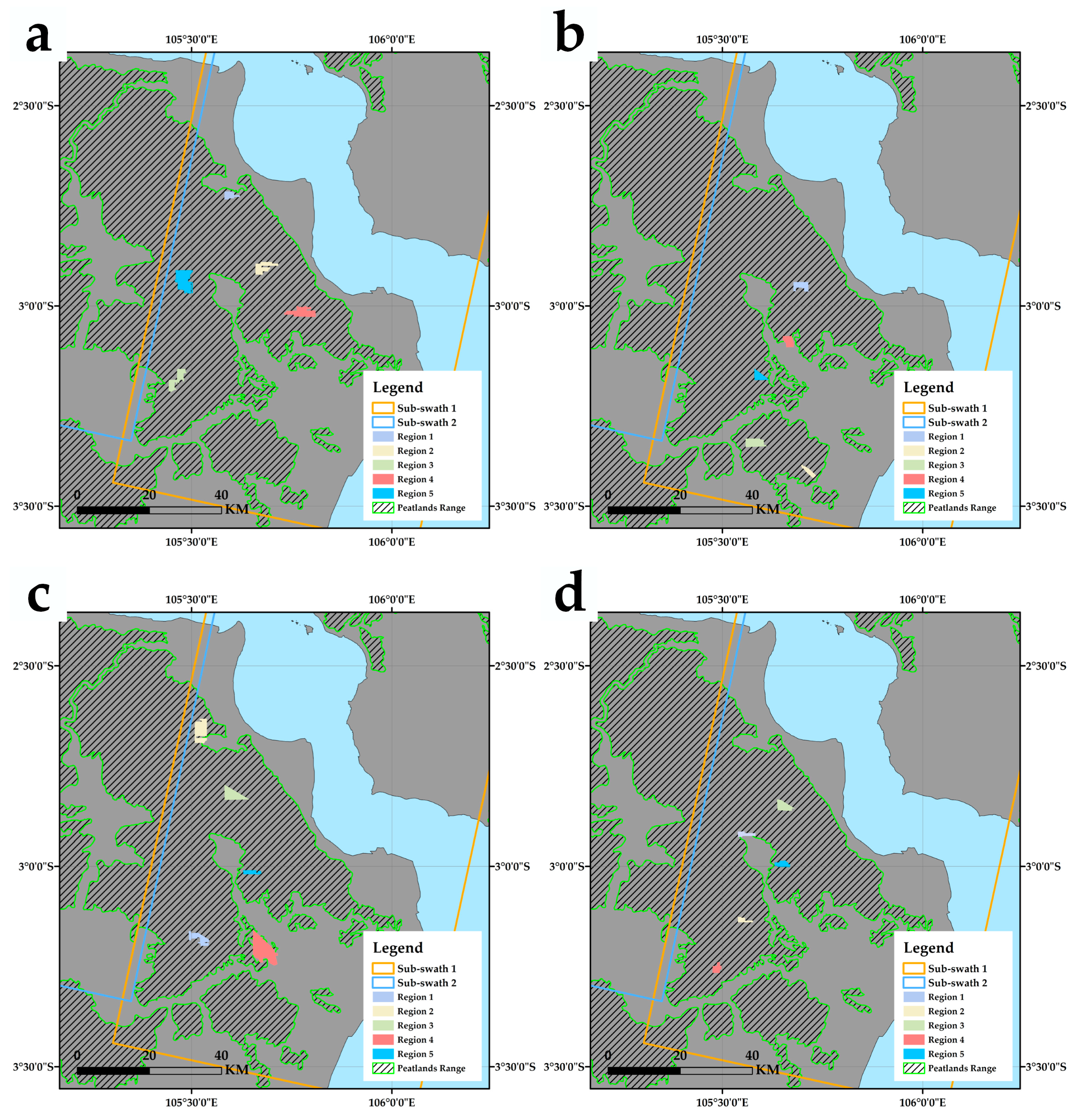
All images in each subset were registered with the master images, and the interferograms were then generated. Regions of peatlands with high coherence characteristics in the interferograms generated by images 12 days apart from the master image were labeled, which were used to analyze the temporal change of peatlands. The SAR images of the four subsets are listed in Table 3. Furthermore, it was necessary to notice that the regions in different subsets were different, they are plotted in Figure 3.
Exponential-based coherence attenuation model, as Equation (2) shows, was introduced to describe the variation of coherence characteristics in peatlands [58,59]:
γ ^ t = γ 0 γ e t τ + γ
where  γ ^ t  is the coherence value,  γ 0  represents the initial coherence of ground objects,  γ  is the long-term coherence, which shows the pixels’ coherence’s convergent value in time series.  τ  is a constant, which means the time that coherence drops down to the  1 e  of initial coherence.
Labeled regions of peatlands in four subsets were employed to fit Equation (2). The fitting curves and parameters were respectively plotted and listed in Figure 4 and Table 4. After analyzing the fitting results, we noticed that:
  • The coherence coefficient of tropical peatlands exhibited a high value during the initial stages of dynamic changes (with  γ 0  approximately 0.54) and decreased with time, approaching incoherence scatterers (with  γ  approximately 0.08) finally. Besides, the coherence decreased slowly in the rainy seasons ( τ  is about 18.5 days in Subset 1, 2, 3, and about 24.5 days in Subset 4).
  • The coherence coefficient’s changes of labeled regions during the same period were also different. Such as in Subset 2, the coherence coefficient in regions 2 and 3 dropped to about 0.1 with 24-day time threshold, but region 4 still kept a high coherence, which had a similar initial coherence with regions 2, 3.
  • Spatial distribution of regions with high coherence was different within different subsets, so it was hard for peatlands to keep a high coherence for a long time.
The research on the coherence of peatlands in time and space confirmed the dynamic change of peatlands’ coherence, which was the reason why it was difficult to monitor peatlands with classical InSAR technology. Therefore, a novel method was proposed in the following sections to solve this problem. Besides, those findings in this section will guide the processing strategies in monitoring the deformation of peatlands by InSAR.

3.2. Continuous Coherence Three-Dimensional (3D) Model with 12-Day Time Threshold

Different from the amplitude-based method in PS-InSAR [60], the coherence coefficients threshold was utilized in SBAS-InSAR to select high coherence scatterers [61], which increased the density of scatterers while reducing the amount of data processed. Therefore, the continuous coherence 3D model in the temporal dimension was constructed, and the time threshold was set as 12 days because ground objects could keep the maximum coherence under the shortest revisit time of Sentinel-1. Furthermore, we analyzed the temporal decorrelation model of peatlands in Section 3.1 to determine the coherence coefficients threshold (set as 0.2) and optimal time threshold (set as 24 days), which were set based on the following considerations:
The time thresholds that included 12, 24, 36, and 48 days were focused on, and the long-term coherence was set as 0.1, which improved the robustness of the coherence coefficients threshold. We noticed that setting 24 days as the time threshold could obtain interferograms with high reliability because the coefficient thresholds of some regions were lower than 0.1 with a 36- or 48-day time threshold. Furthermore, all regions’ coherence coefficients were higher than 0.2 with a 12-day time threshold and would still keep high coherence (higher than the long-term coherence) with a 24-day time threshold.
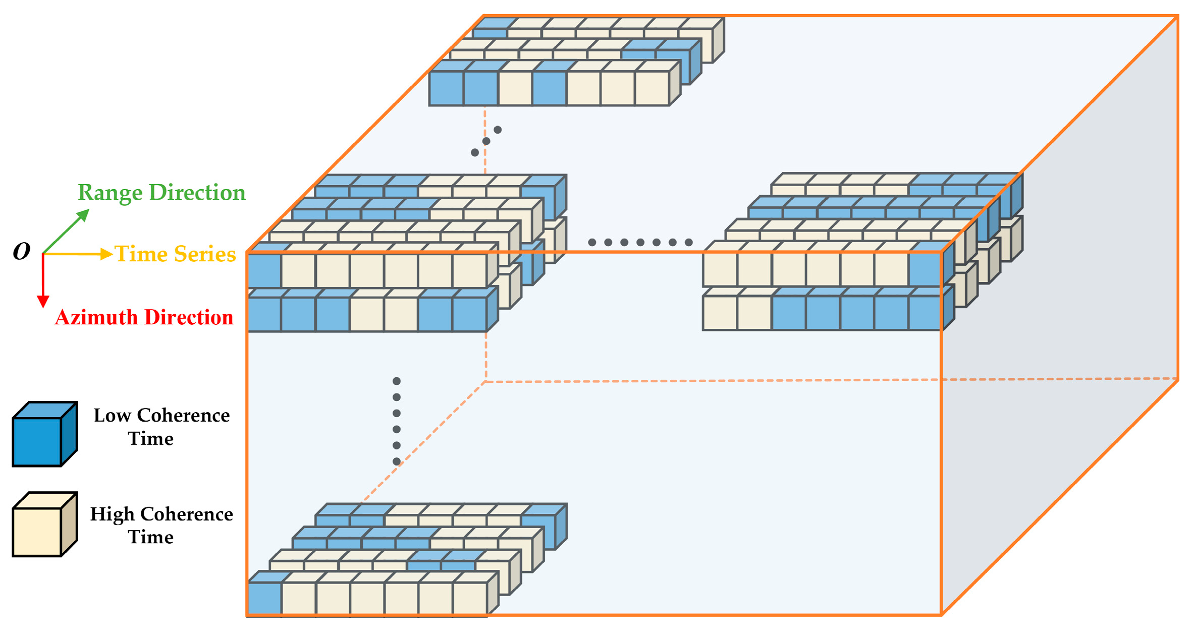
Finally, pixels with coherence coefficients higher than the coherence coefficients threshold (0.2) were set as high coherence time points, and lower were set as low coherence time points in the time series. An example of the continuous coherence 3D model with a 12-day time threshold is shown in Figure 5.

3.3. Construction of Adaptive HCTSs

The construction of temporal subsets primarily comprises four elements: start time of HCTSs, time span of HCTSs, stop time, and the step length between temporal subsets. Subsequently, four elements will be analyzed in detail.
  • Start time of HCTS: HCTS will start with the first SAR image in the whole time series.
  • Time span of HCTSs: Cigna et al. [37] established the correlation between the velocity standard errors and the number of interference pairs, as shown in Equation (3). Based on the empirical correlation, the minimum number of interferograms ( N i ) required for a temporal subset can be calculated by setting an acceptable maximum error.
    ε v e l = M N i
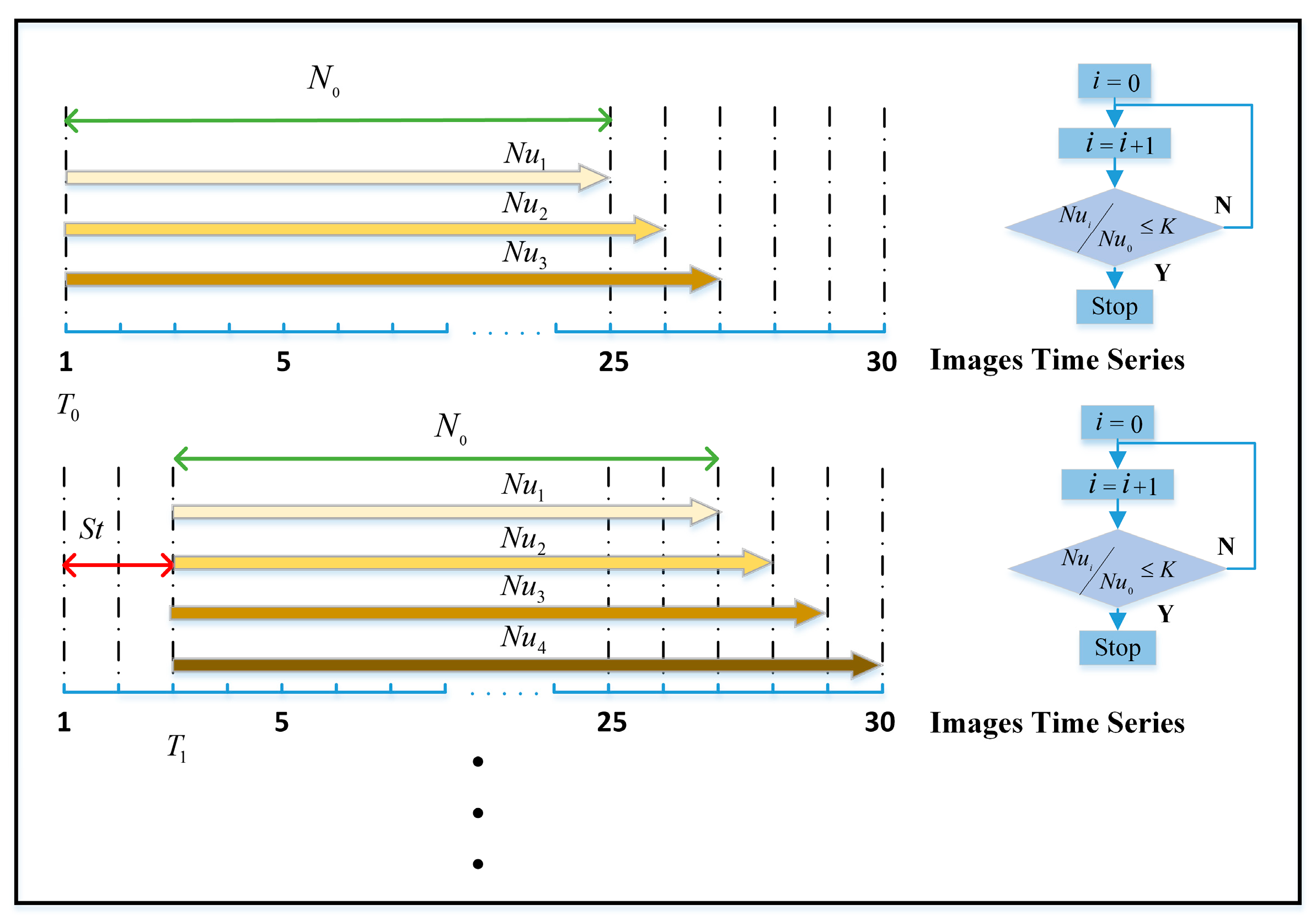
  • Stop time of HCTSs: An initial time subset has been established based on the aforementioned elements, but subsets require more SAR images because more interferograms (more observations) can reduce the error of the rate. However, it is necessary to realize that pixels’ coherence may be hard to keep high coherence for a longer time because there are more uncertainties. Therefore, taking into account the relationship between the length and number of TCSs in the temporal subset holistically, a method is proposed to create adaptive temporal subsets, which utilize the change of measurement points to optimize stop time. The detailed process is as follows:
Step A: Firstly, the number of pixels with high coherence ( N u 1 ) that can be obtained is calculated based on the minimum span requirement and the continuous coherence 3D model established in Section 3.2.
Step B: A subsequent SAR image is added to the end of the temporal subset, resulting in a new temporal subset. The interferometric combination is updated, and the number of pixels ( N u i ) obtained in this new subset is calculated.
Step C: In order to get the upper limit for adding images, the judgment criterion is set to terminate the infinite extension of the temporal subset: If  N u i / N u 1 < K  is true, it is time to stop adding SAR images, where  K  is a proportionality constant, which is related to the actual situation. The equation refers to the reduction proportion of integrated pixels relative to the initial temporal subset.
Step D: In case step C is false, iterate through steps B and C until either step C becomes true or there are no further images available in the whole time series.
4.
Step length between temporal subsets: HCTS is established after completing the above steps. However, it is necessary to recognize that there are multiple temporal subsets rather than only one in the whole time series in most cases. Step length between temporal subsets needs to be considered because starting with each SAR image will produce many temporal subsets, which will slow down the efficiency of InSAR processing in large-scale and long-time series monitoring.
To solve this problem, the time threshold is introduced as the step length between temporal subsets, and TCSs can keep high coherence without losing too many interferograms under the 24-day time threshold. Therefore, while including as many measurement points as possible in the deformation results, the number of HCTSs is reduced, and the processing efficiency is improved. Construction of adaptive HCTSs has been achieved, as exemplified in Figure 6. The SAR images will be added to the subset orderly, and the number of pixels with high coherence in the current subset will be recalculated, and the flowchart on the right will be used to determine whether the termination condition is met. Then, the process will be repeated following Step 4.
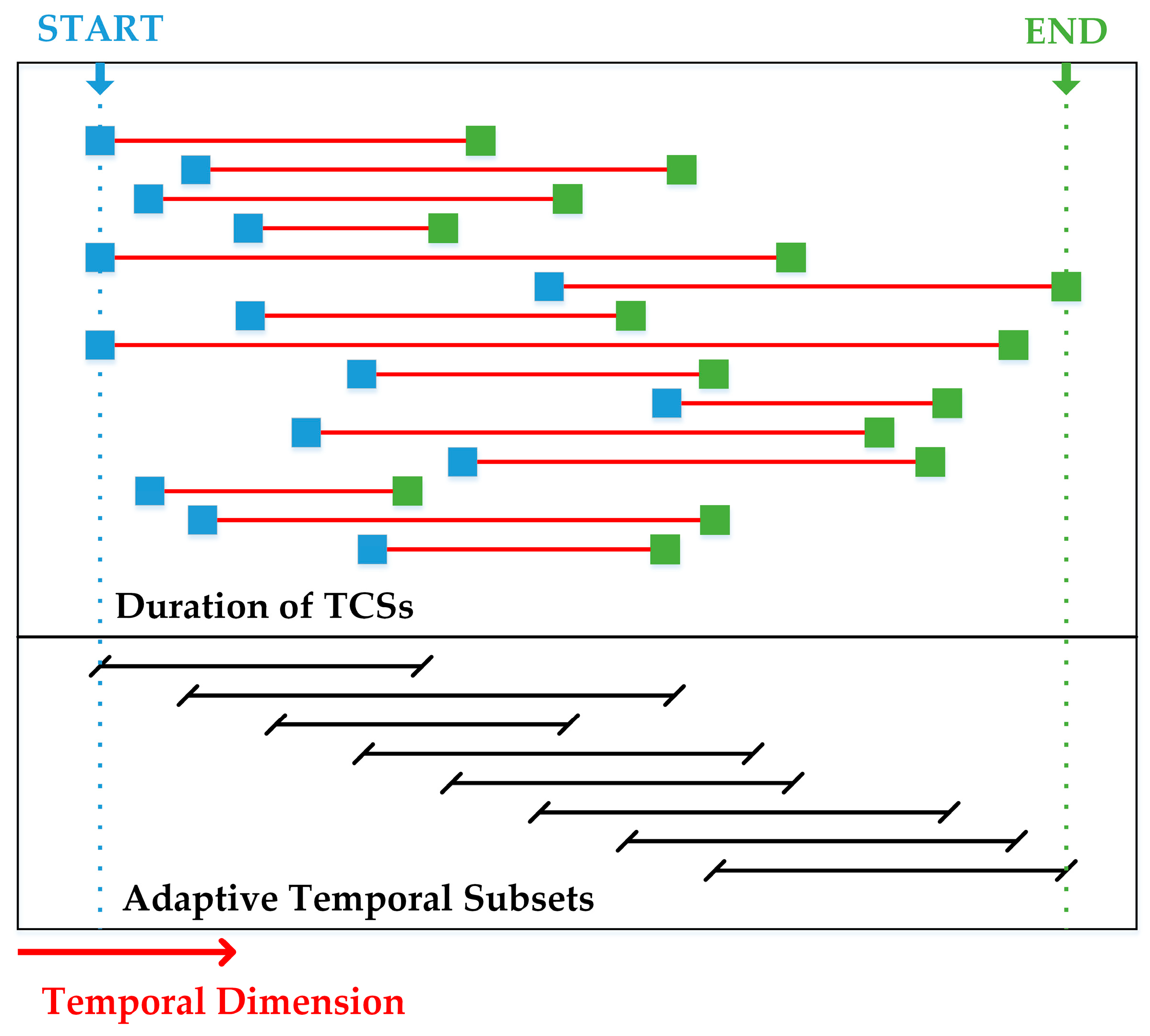
Figure 7 shows the establishment of adaptive HCTSs based on the above method for TCSs with different high coherence durations in the whole time series, and each unit possesses its own duration of high coherence.

3.4. SBAS-InSAR Processing with Time-Weighted in HCTSs

Multiple HCTSs are established for the whole time series of Sentinel-1 images after Section 3.3. Generic Mapping Tools Synthetic Aperture Radar software (GMTSAR) [62] is utilized to process Sentinel-1 images and generate interferograms (gmtsar/gmtsar: GMTSAR (github.com), accessed on 20 March 2023). With the precise orbit data provided by ESA, SAR images within the HTCSs are accurately co-registered to the master images. Furthermore, the space-time baseline map and interferograms are generated with a reasonable spatial threshold and time threshold. For the same pixel  P  in two SAR images, the interferometric phase  φ P  of pixel  P  in interferograms could be described as Equation (4) [63]:
φ P = φ d e f + φ t o p o + φ a t m + φ o r b + φ n o i s e
where  φ d e f  is the phase change caused by the displacement of ground object in the line of sight of radar during two observations,  φ t o p o  is the residual topographic phase due to the error in the digital elevation model (DEM),  φ a t m  is the atmospheric phase disturbance,  φ o r b  and the  φ n o i s e  are respectively the satellite orbital error and the random noise error.
In order to improve the coherence of ground object pixels and reduce the influence of speckle noise, multi-view processing with azimuth direction 2 and distance direction 8 is adopted. The 1-arcsecond (about 30 m resolution) Shuttle Radar Topography Mission (SRTM) DEM is used to remove topographic phase contribution, and the interferograms were unwrapped by calling SNAPHU [64]. The atmospheric phase delay is removed by common-point stacking.
After the above operations, the interferometric phase can be expressed as Equation (5):
φ P = 4 π λ [ D p T B D p T A ]
where the  λ  is radar wavelength, and  D p T A  and  D p T B  mean the pixel  P ’s displacement in Time  A  and  B .
Convert Equation (5) into matrix form:
φ ( M · 1 ) = B ( M · N ) V ( N · 1 )
where  B ( M · N )  is a coefficient matrix with  M · N M  is the number of interference pairs,  N  corresponds to the number of SAR images, and the  V ( N · 1 )  is the deformation rate at a different time, which could be expressed as Equation (7)
V T = [ V 1 = φ 1 T 1 T 0 , , V N = φ N φ N 1 T N T N 1 ]
Then, based on the singular value decomposition (SVD) method of the matrix, the linear deformation rate of a pixel in the subset time is calculated, and the cumulative deformation is generated by integrating in the temporal dimension. After geocoding with the SRTM DEM, pixels are converted from radar coordinates to geographic coordinates (WGS84). Furthermore, stable reference points are selected to convert the relative deformation rate of pixels to the absolute deformation rate. We assumed that the deformation of the peatlands is mostly vertical, so it is necessary to project the line-of-sight displacement deformation ( d L O S ) to the vertical displacement deformation ( d v e r ). This transformation is achieved by obtaining the incidence angle ( θ ) of the Sentinel-1 and calculated based on Equation (8):
d v e r = d L O S cos θ
Since the deformation results of a single time subset are scattered in time and limited in space coverage, we obtain the average deformation rate of peatlands in the whole time series and each natural year interval through temporal dimension weighted processing as Equation (9) shows:
V a v e = i = 1 M V i T i i = 1 M T i
where  V a v e  is the average deformation rate in mm/year, and  M  is the number of high coherence temporal subsets,  V i  and  T i  are respectively the rate of deformation and time span in  i - t h  HCTS.

3.5. Reliability Analysis of the Deformation Rate

In this study, the Pearson product-distance correlation coefficient (Pearson’s r) and Root Mean Square Error (RMSE) are calculated to evaluate the reliability of the deformation results, which are respectively defined as the following equations:
P e a r s o n s   r = i = 1 N ( X i X ¯ ) ( Y i Y ¯ ) i = 1 N ( X i X ¯ ) 2 i = 1 N ( Y i Y ¯ ) 2
where  X i  and  Y i  are deformation rate in two sub-swaths, respectively.  X ¯  and  Y ¯  are the mean deformation rate in two sub-swaths, and  N  is the total number of measurement points.
R M S E = 1 N i = 1 N ( X i Y i ) 2
where the meaning of parameters in Equation (11) is same as in Equation (10).
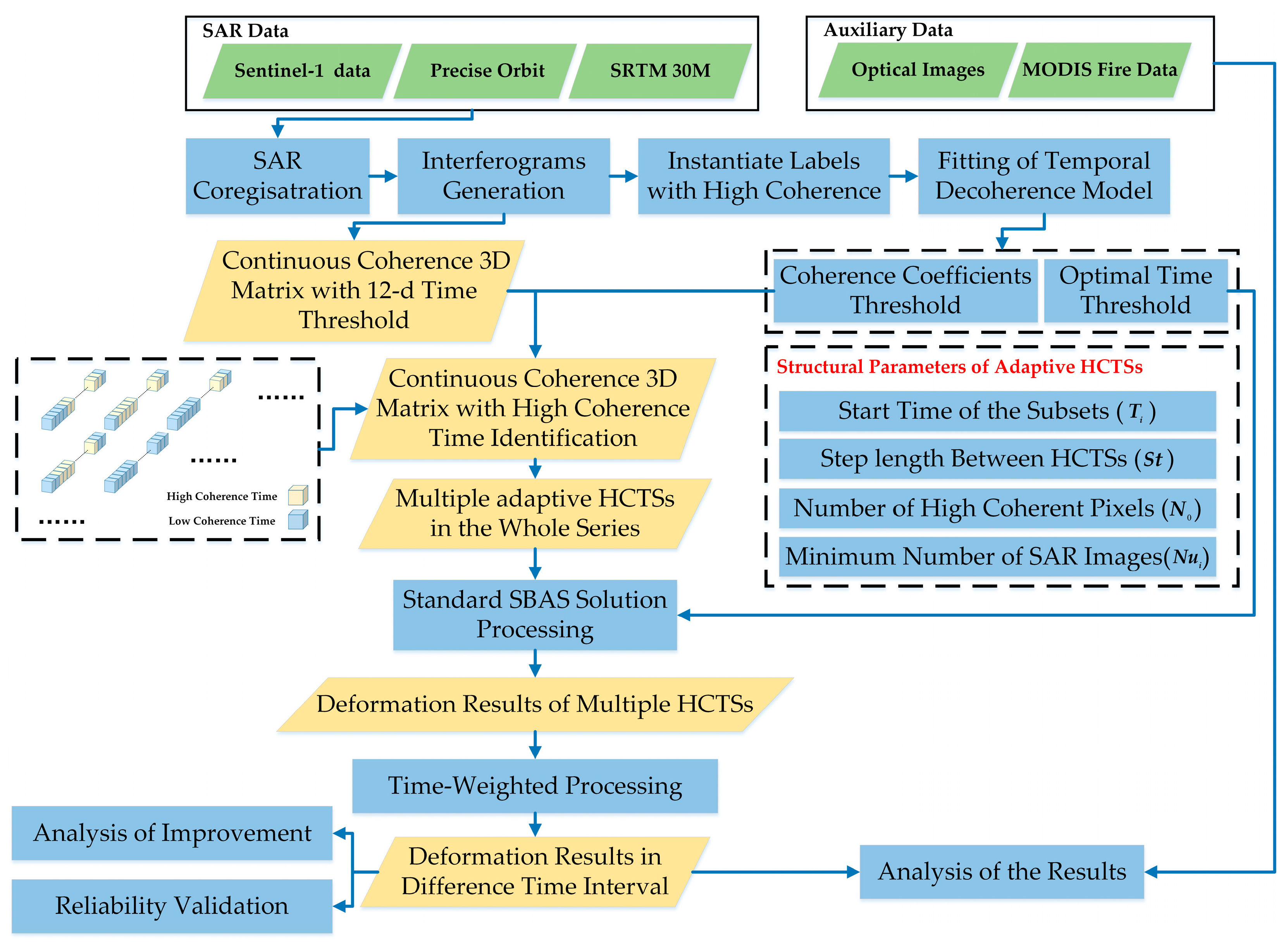
Finally, the overall experimental process is summarized as follows (Figure 8):

4. Results and Analysis

4.1. Results of the Adaptive HCTSs

Ninety Sentinel-1 SAR images over South Sumatra province were processed and generated the adaptive HCTSs based on the method proposed in Section 3.3. The general parameter M was set as 11 in [37], which was accepted in our experiments. We comprehensively considered the number of SAR images and temporal subsets and set the maximum acceptable standard error as 2.5 mm/year, so a minimum of 20 interferograms were required in a subset. Besides, considering the relatively reliable time threshold was set as 24 days in Section 3.2, the minimum length for temporal subsets generally required about 11 SAR images. In order to keep data continuity in the temporal subsets, some SAR images with a 36-day time threshold were added, while far-apart isolated images were ignored. The proportionality constant  K  was set as 0.8, which was empirically determined in the experiments, and the results of adaptive HCTSs in Sub-swath 1 and Sub-swath 2 were listed in Table 5. Note that the third HCTS in both sub-swaths were reserved, though there were only eight images, because we did not want to lose too many images.

4.2. Deformation Results of Peatlands in South Sumatra Province from 2019 to 2022

Adaptive HCTSs presented in Section 4.1 were utilized to obtain the deformation results, and the time threshold and spatial baseline threshold were respectively set as 24-day and 300 m, which could obtain the high-quality interferograms as much as possible and increase the number of interferograms.
Reference points in two sub-swaths were selected in  P 1  (Sub-swath 1) and  P 2  (Sub-swath 2), both located in the urban areas, which are generally considered to be more stable than natural surfaces [30].  P 2  is near a Global Positioning System (GPS) Station (Station ID: PAL8, http://geodesy.unr.edu/NGLStationPages/stations/PAL8.sta, accessed on 20 March 2023). Since the station only updated to 2017, the information provided by the GPS station was not used to correct the deformation results. Details of the reference points are shown in Table 6.
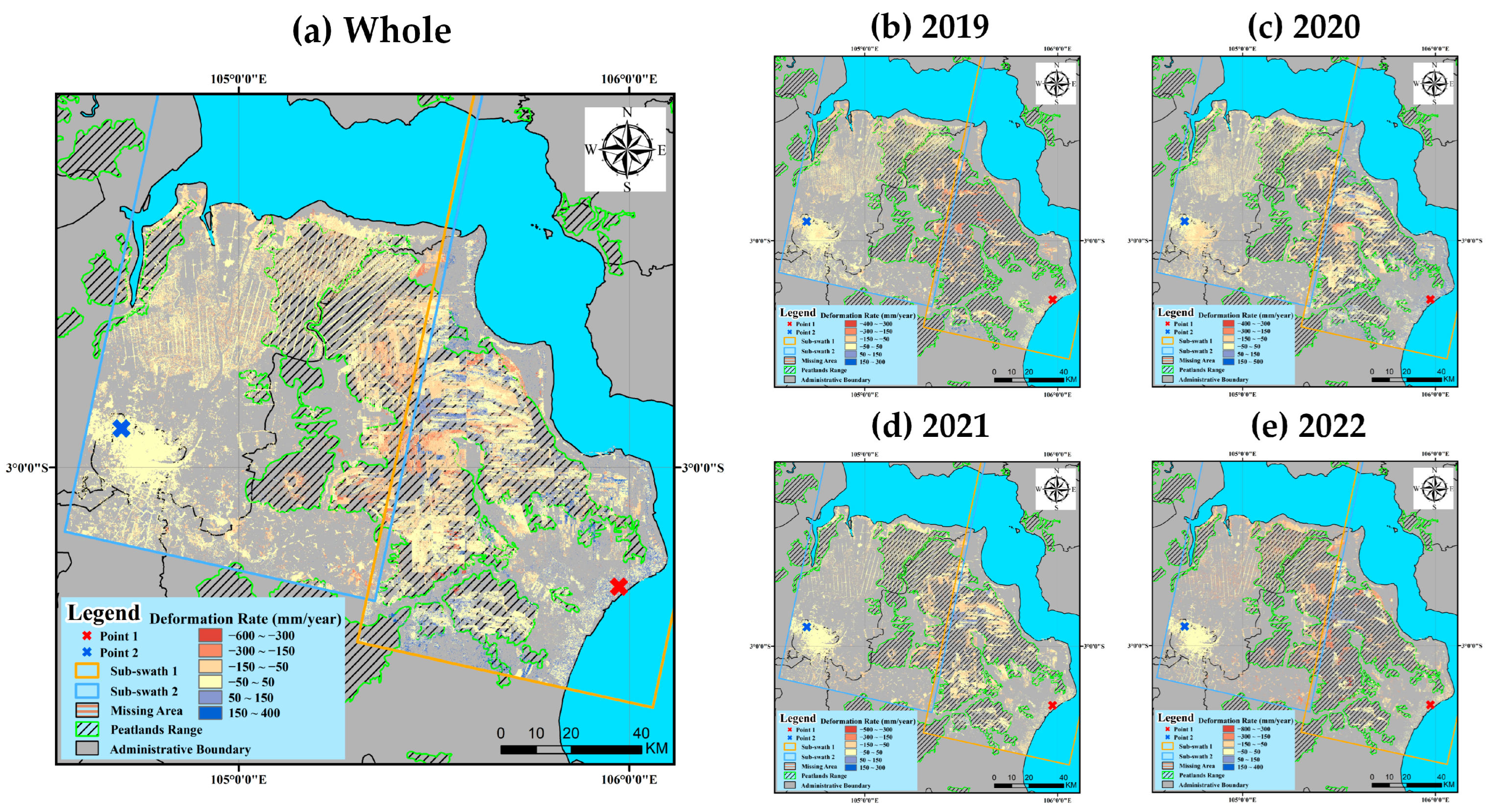
The deformation results of South Sumatra province’s peatlands from 2019 to 2022 are shown in Figure 9. The time-weighted method was used to generate deformation results of natural year interval and the whole time series (from 2019 to 2022, and we call it Whole) based on the multiple temporal subsets, which will be utilized in the following analysis and discussions. Moreover, it is necessary to note that the negative deformation value represented the subsidence in peatlands, and the positive value meant the uplift.
The study found that most of the peatlands in South Sumatra province continued to experience extensive and severe degradation between 2019 and 2022, and the distribution of subsidence characteristics was closely related to the scope of peatlands in space. Approximately 43.5% of pixels in peatlands exhibited subsidence (less than −50 mm/year), while 45.8% kept stable (between −50 mm/year and 50 mm/year), and the remaining 10.7% displayed uplift (greater than 50 mm/year), which accounted for a small proportion, so we did not focus on these in this paper. Details of deformation results in the peatlands are listed in Table 7.
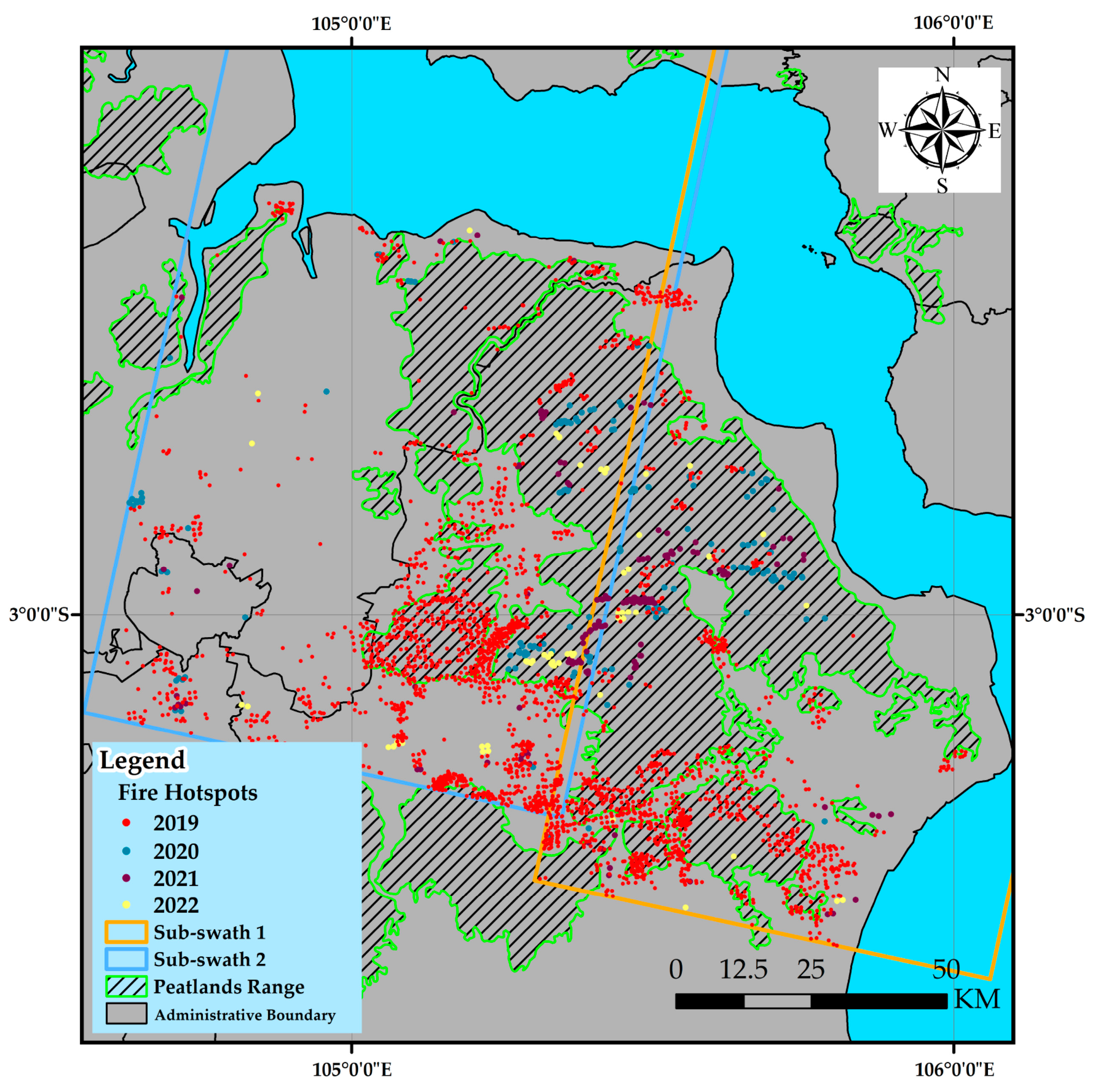
Compared with deformation results in 2019 and 2022, the number and coverage of measurement points obtained in 2021 and 2022 significantly increased. By comparing the deformation results spatially and quantitatively with fire hotspots provided by MODIS in South Sumatra province from 2019 to 2022 (Figure 10), the above findings should be due to the decrease of the vegetation cover of industrial plantations caused by the dense fire hotspots in 2019, and the large bare land greatly increased the number of measurement points in 2020 and 2021. By 2022, most of the fire-affected areas have been vegetated again, so the number of measurement points was relatively small.
The average deformation rate of the peatlands in South Sumatra province ranged from about −567 to 347 mm/year and showed a higher deformation rate in 2019 and 2022. The higher deformation rate in 2019 was due to the increased oxidation of peatlands, which was caused by the extensive and intensive fires. While there was a large amount of consolidated soil in the upper layer caused by the oxidation (burning) of the previous year, which slowed down the oxidation process to a certain extent and resulted in a decrease in the deformation rate. At the same time, replanting in late 2020 may plow up the consolidated and burned soil, and the rapid oxidation of the underlying fresh peatlands soil resulted in an increase in the deformation rate in 2021.
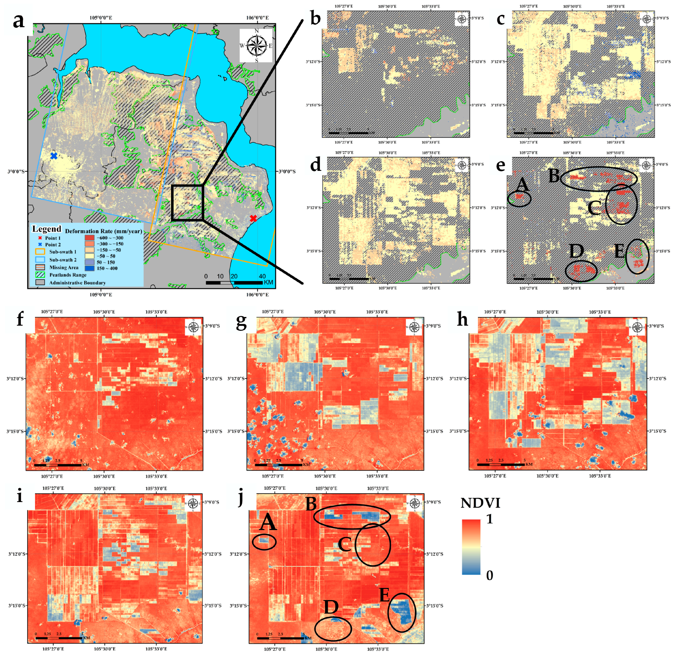
Finally, the region that appeared to have a relatively high deformation rate in 2022 was focused on and the historical deformation results (2019 to 2021) are shown in Figure 11b–e. Five parts (A–E) of the region were focused on and there were a few optical images with better imaging due to the cloud conditions, so normalized vegetation index (NDVI) maps at different times were created to replace the changes of NDVI in the whole time series. Most parts kept the relatively high vegetation cover until 2022, which resulted in the lack of historical deformation results. Specifically speaking, part A and E kept a high and stable vegetation cover in the past three years. The higher deformation rate in 2022 may be caused by the drainage operations in the new industrial plantations, which is similar to the rate in the first year after drainage [16]. Then, part B and C showed a low vegetation cover in 2019 and 2022 and a higher deformation rate in 2022, which may be caused by the further development of industrial plantations. Finally, part D, due to the limitation of optical image imaging time, the lower vegetation cover was not observed in the NDVI maps generated in 11 April 2022, although part D showed a higher deformation rate in the result of 2022.

4.3. Reliability Validation of the Peatlands’ Deformation Results

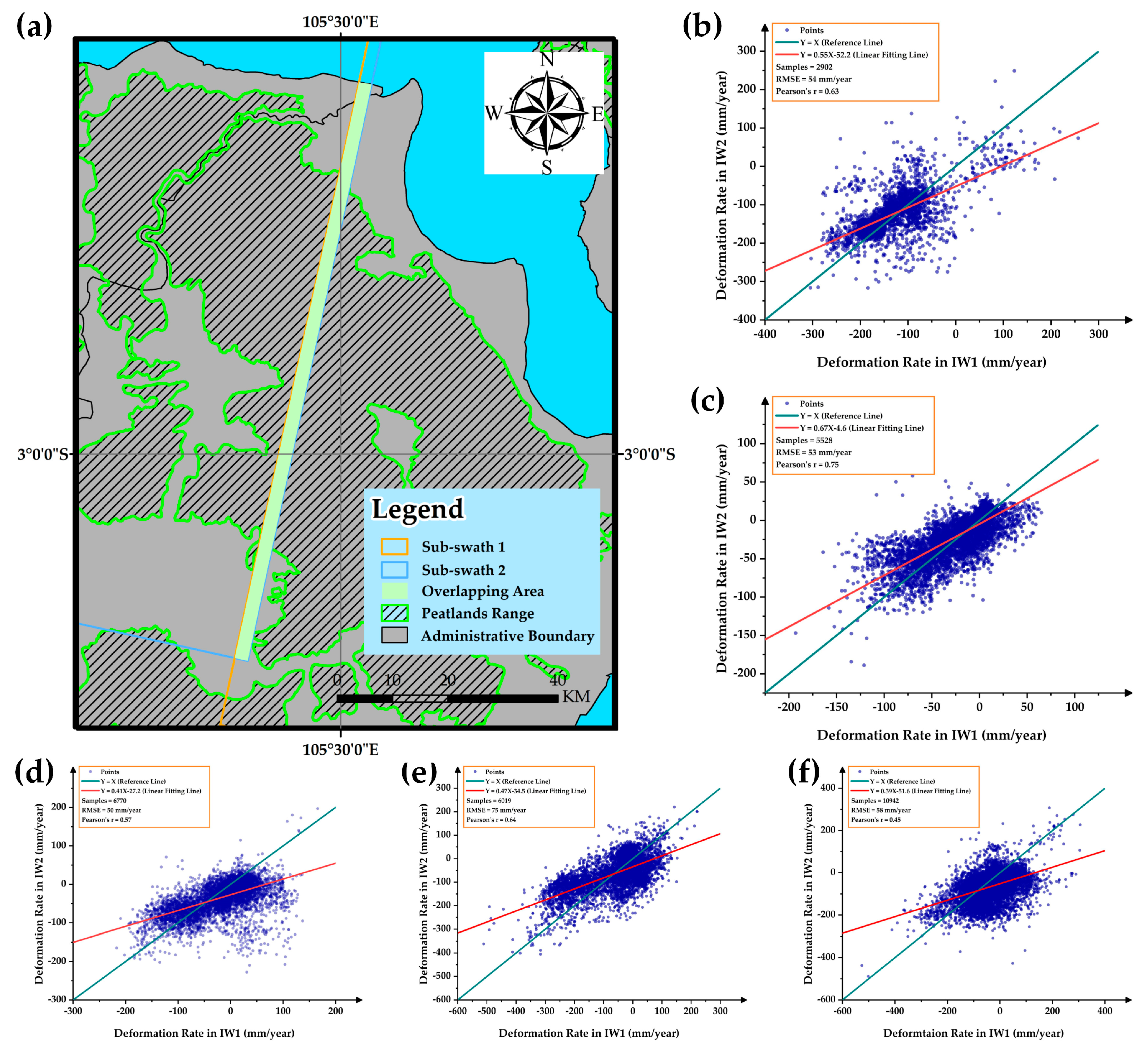
Tropical peatlands are mostly located in areas covered by dense vegetation and hard to access, so field ground leveling is difficult, and the local GNSS data available are limited at the same time. Therefore, the method to validate peatland’s deformation results used in [30] was applied in our experiments, Pearson’s r and RMSE of the average deformation rate in the overlapping area’s deformation results were calculated and analyzed to validate the reliability of results.
The deformation results of natural year (2019, 2020, 2021, 2022) and the whole time series obtained by time weighting (Whole) were verified. As shown in Figure 10, Pearson’s r ranged from 0.44 to 0.75, indicating a relatively strong linear relationship between deformation results in the overlapping region. RMSE ranged from 50 to 75 mm/year, which reflected the degree of deviation between the deformation results and was acceptable relative to the overall range of deformation rate. Those parameters proved that the deformation results provided by the proposed method were reliable. Besides, Pearson’s r in Figure 12f was relatively low, which may be due to the increased instability caused by more data being weighted, and the relatively high RMSE in Figure 12e was affected by the higher degree of dispersion of deformation results.

4.4. Comparison and Evaluation of Deformation Results of Adaptive HCTSs SBAS-InSAR

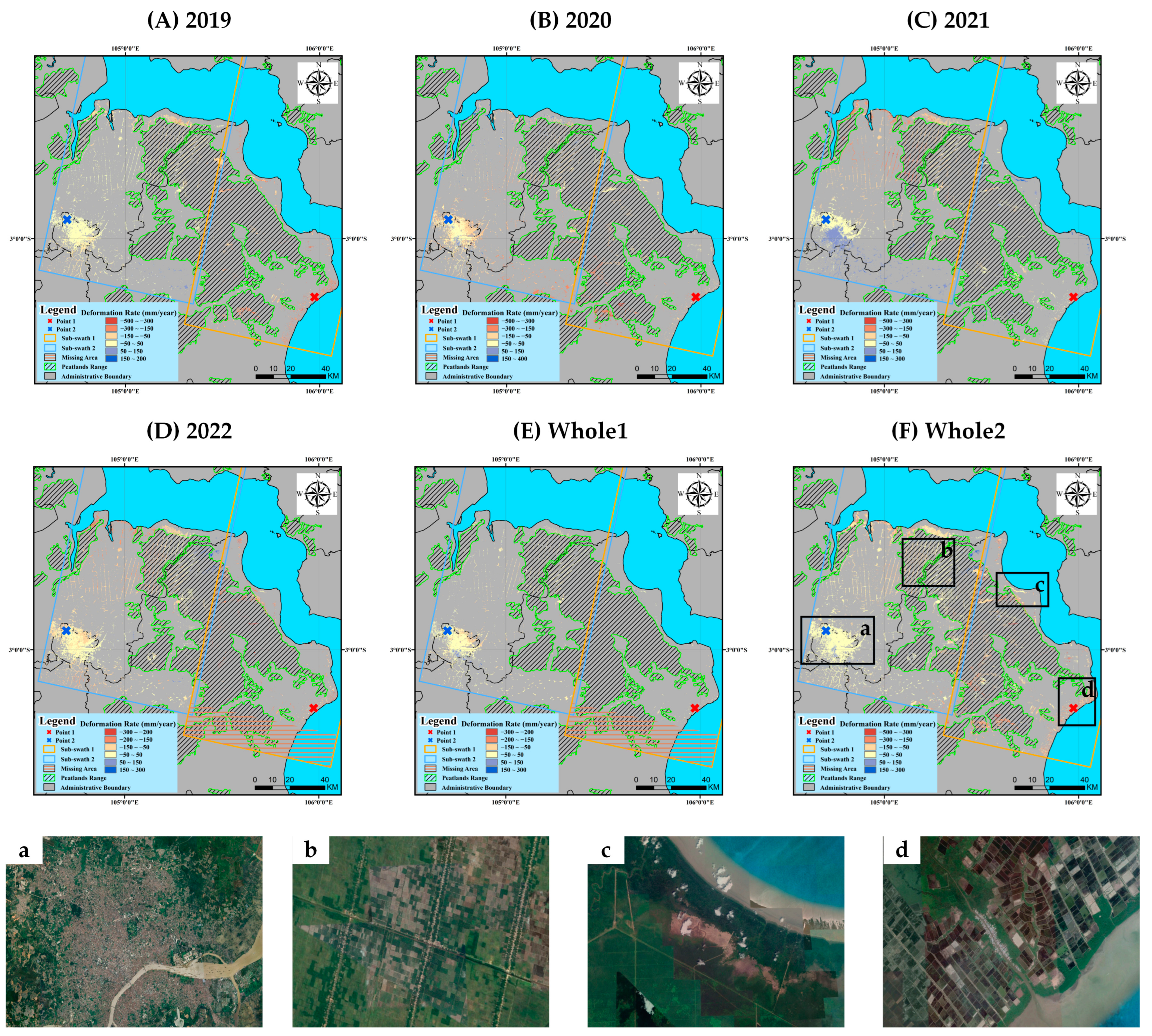
To evaluate the improvement of the proposed method, comparisons between SBAS-InSAR and HCTSs SBAS-InSAR were conducted in three parts: Firstly, the SAR images in the whole time series were utilized for computation (call it Whole 1). Secondly, datasets divided with the natural year were computed separately. Finally, based on the above results, the time-weighted approach was employed to obtain deformation results in the whole time series (call it as Whole 2). Temporal and spatial baselines in all experiments were consistent (24 days and 300 m), and some SAR images with a 36-day time threshold were added to the subsets due to the absence of SAR images in certain time periods. Besides, the range of some SAR images in 2022 does not fully overlap with the main SAR image, which resulted in the loss of measurement points in the deformation result of 2022 and the whole time series.
Deformation results obtained in comparative SBAS-InSAR experiments are presented in Figure 13.
Comparative SBAS-InSAR experiments showed that the number of measurement points was limited and primarily concentrated in PS scatterers when utilizing all SAR images or subsets of time divided by natural year as input data. Those were exemplified in Figure 13, (a) Palembang City, (b) artificial roads within plantations, (c) soil that stays bare for a long time, and (d) towns. Improvement of the number and the coverage area of measurement points between adaptive HCTSs SBAS-InSAR method and the SBAS-InSAR methods are plotted in Figure 14. Statistics of the comparative information are listed in Table 8. Note that Whole 1 and Whole 2 were both compared with the Whole.
Adaptive HCTSs SBAS-InSAR obtained a larger number of measurement points compared with the SBAS-InSAR methods. Those newly acquired measurement points were primarily located in the areas where SBAS-InSAR methods had difficulty obtaining, such as industrial plantations with significant changes in vegetation cover in a short time. According to the detailed comparative information, the number of measurement points in a single natural year increased about 2 to 12 times, and the ratio of coverage increased from 1.8% to 30.4%. Compared with the deformation results in Whole 1 and Whole 2, the number of measurement points increased about 6 to 127 times and 2 to 6 times, respectively. Furthermore, there was a significant improvement, especially in Sub-swath 1. The improvement was relatively low in Sub-swath 2 due to the relatively low change in plantation forests in this region and the long-term stability of the southern forests. Even with the adaptive HCTSs SBAS-InSAR method, it was still challenging to obtain satisfied deformation results.

5. Discussion

Rapid degradation of tropical peatlands has released a large amount of greenhouse gas, which accelerates the process of global warming [65,66]. Aiming at the limitations of classical InSAR technology in the research of peatland degradation, this paper constructed multiple adaptive HCTSs by capturing the dynamic variation range of peatlands, which made full use of the limited phase information to calculate the deformation rate and the time-weighted strategy was utilized to get the deformation results in corresponding time intervals based on the discrete HCTSs.
The proposed method was practiced in the South Sumatra province and revealed the widespread and rapid degradation of peatlands from 2019 to 2022 (about −567 to 347 mm/year). Based on the average annual deformation rate of peatlands, the degradation law of peatlands in a long time after fires was inferred. In addition, Pearson’s r and RMSE of deformation results in overlapping areas were calculated to verify the reliability of the results. We compared the results with previous studies of the region. Specifically speaking, the subsidence rate in [36] was relatively higher (25 cm/year before fires and 1.6 m/year after fires), which should be related to the initial degraded state of peatlands and the more serious fires. Then, the deformation rate in [31] was consistent with us in the same region, but we observed a higher deformation rate in the region that did not be obtained in [31].
As shown by the comparisons with SBAS-InSAR methods, adaptive HCTSs SBAS-InSAR effectively increased the density of measurement points (2 to 127 times). Besides, compared with the ISBAS method in [37], this short-time baseline, multi-time subset method significantly reduced the number of interferograms (from about 18%~31% of all possible interference combinations to about 5% of all), and the memory requirements and the reduction will be more significant in a longer time series. The proposed method has strong extensibility. Construction parameters of HCTSs could be updated dynamically by combining with the coherence characteristics of different ground objects, the precision of results, and the number of images to extend the deformation monitoring ability of the proposed method in various ground objects.
Although HCTSs SBAS-InSAR method has been able to obtain a largerand relatively reliable number of measurement points, it still has certain limitations: Firstly, it is still difficult to obtain the deformation information of the completely incoherent regions in the whole time series, such as the dense forest or the stable state industrial plantation above the original peatlands. Besides, the overall process of the proposed method is relatively complicated and needs to be simplified.

6. Conclusions

An adaptive HCTSs SBAS-InSAR method is proposed to address the problem that the dynamic changes of vegetation cover in tropical peatlands make it difficult to obtain surface deformation information by classical InSAR methods. Ninety Sentinel-1 SAR images (2019−2022) were processed, and the spatial and temporal degradation of peatlands in South Sumatra province were revealed based on the proposed method. Besides, the reliability of the deformation results was evaluated by calculating Pearson‘s r and RMSE, and the proposed method was compared with the SBAS-InSAR methods to evaluate the improvement. The conclusions of this paper are summarized as follows:
  • Based on the deformation results, the widespread and rapid degradation of peatlands in South Sumatra province between 2019 and 2022 was observed, with the deformation rate ranging from −567 to 347 mm/year. The spatial distribution of subsidence was closely related to the scope of peatlands.
  • The study found that peatlands’ deformation rate and the number of measurement points were affected by fires and the change in land cover. Fires caused higher rates of peatland deformation, after which the rate of deformation decreased slightly and then increased with time. At the same time, the change in land cover, such as the newly reclaimed industrial plantation, also contributed to the rapid deformation of peatlands. Besides, the number of measurement points increased after fires or deforestation because there is a lot of soil exposed and decreases with the restoration of vegetation.
  • Pearson’s r and RMSE in overlapping area’s deformation results ranged from 0.44 to 0.75 and 50 to 75 mm/year, respectively, which verified the reliability of the proposed method. In addition, compared with the deformation results obtained by SBAS-InSAR methods, the number of measurement points increases by about 2 to 127 times, and the ratio of coverage increases from 1.8% to 41.9%. New measurement points were always located in the areas that were difficult to monitor with SBAS-InSAR methods, which enhanced the monitoring ability of InSAR technology in tropical peatlands. At the same time, the number of interferograms and storage requirements were significantly reduced compared with the ISBAS method, which was conducive to meeting the requirements of calculation in a wider range.
In the future, the adaptive HCTSs SBAS-InSAR method will be improved and applied to the calculation of peatland degeneration across Southeast Asia in recent years. Then, the emission of carbon dioxide caused by the peatland degeneration will be estimated according to the relationship between them. Finally, we will assess the extent to which the degradation of tropical peatlands in Southeast Asia contributes to global climate change.

Author Contributions

Conceptualization, X.Z., C.W. and Y.T.; data curation, X.Z., T.L., L.Z. and S.G.; formal analysis, X.Z. and Y.T.; methodology, X.Z. and C.W.; software, X.Z., C.W. and Y.T.; validation, X.Z. and Y.T.; writing—original draft, X.Z.; writing—review and editing, C.W. and H.Z.; visualization, X.Z.; supervision, C.W.; project administration, C.W. and H.Z.; funding acquisition, C.W. All authors have read and agreed to the published version of the manuscript.

Funding

This work is supported by the National Natural Science Foundation of China under Grant 41930110.

Data Availability Statement

Global peatlands’ distribution is downloaded from the website of Global Peatlands provided by the GlobalForestWatch (http://gfw2-data.s3.amazonaws.com/commodities/zip/peat_lands.zip/, accessed on 1 April 2023). Sentinel-1 SAR images could be obtained in the ASF provide by the European Space Agency (https://search.asf.alaska.edu/, accessed on 1 April 2023). Landsat optical images are provided by the Earth Explorer (https://earthexplorer.usgs.gov/, accessed on 15 April 2023). Additionally, GMTSAR open source software could be download in the GitHub (gmtsar/gmtsar: GMTSAR (github.com), accessed on 20 March 2023). Finally, MODIS fire data is available at (https://firms.modaps.eosdis.nasa.gov/map, accessed on 1 May 2023).

Acknowledgments

Author would like to thank the European Space Agency for providing the Sentinel-1 SAR data and the DEM data provided by SRTM. Besides, thank the GMTSAR open source software and the Landsat optical images and MODIS fire data provided by USGS.

Conflicts of Interest

The authors declare no conflict of interest.

References

  1. Brown, L.E.; Holden, J.; Palmer, S.M.; Johnston, K.; Ramchunder, S.J.; Grayson, R. Effects of fire on the hydrology, biogeochemistry, and ecology of peatland river systems. Freshw. Sci. 2015, 34, 1406–1425. [Google Scholar]
  2. Kirpotin, S.N.; Antoshkina, O.A.; Berezin, A.E.; Elshehawi, S.; Feurdean, A.; Lapshina, E.D.; Pokrovsky, O.S.; Peregon, A.M.; Semenova, N.M.; Tanneberger, F. Great Vasyugan Mire: How the world’s largest peatland helps addressing the world’s largest problems. Ambio 2021, 50, 2038–2049. [Google Scholar] [PubMed]
  3. Dohong, A.; Abdul Aziz, A.; Dargusch, P. A review of techniques for effective tropical peatland restoration. Wetlands 2018, 38, 275–292. [Google Scholar]
  4. Wu, J. Response of peatland development and carbon cycling to climate change: A dynamic system modeling approach. Environ. Earth Sci. 2012, 65, 141–151. [Google Scholar]
  5. Temmink, R.J.; Lamers, L.P.; Angelini, C.; Bouma, T.J.; Fritz, C.; van de Koppel, J.; Lexmond, R.; Rietkerk, M.; Silliman, B.R.; Joosten, H. Recovering wetland biogeomorphic feedbacks to restore the world’s biotic carbon hotspots. Science 2022, 376, eabn1479. [Google Scholar] [PubMed]
  6. Humpenöder, F.; Karstens, K.; Lotze-Campen, H.; Leifeld, J.; Menichetti, L.; Barthelmes, A.; Popp, A. Peatland protection and restoration are key for climate change mitigation. Environ. Res. Lett. 2020, 15, 104093. [Google Scholar]
  7. Dise, N.B. Peatland response to global change. Science 2009, 326, 810–811. [Google Scholar] [CrossRef]
  8. Gorham, E.; Lehman, C.; Dyke, A.; Clymo, D.; Janssens, J. Long-term carbon sequestration in North American peatlands. Quat. Sci. Rev. 2012, 58, 77–82. [Google Scholar]
  9. Page, S.E.; Rieley, J.O.; Banks, C.J. Global and regional importance of the tropical peatland carbon pool. Glob. Chang. Biol. 2011, 17, 798–818. [Google Scholar]
  10. Jauhiainen, J.; Hooijer, A.; Page, S. Carbon dioxide emissions from an Acacia plantation on peatland in Sumatra, Indonesia. Biogeosciences 2012, 9, 617–630. [Google Scholar]
  11. Miettinen, J.; Shi, C.; Liew, S.C. Land cover distribution in the peatlands of Peninsular Malaysia, Sumatra and Borneo in 2015 with changes since 1990. Glob. Ecol. Conserv. 2016, 6, 67–78. [Google Scholar] [CrossRef]
  12. Koh, L.P.; Miettinen, J.; Liew, S.C.; Ghazoul, J. Remotely sensed evidence of tropical peatland conversion to oil palm. Proc. Natl. Acad. Sci. USA 2011, 108, 5127–5132. [Google Scholar] [CrossRef] [PubMed]
  13. Hoyt, A.M.; Chaussard, E.; Seppalainen, S.S.; Harvey, C.F. Widespread subsidence and carbon emissions across Southeast Asian peatlands. Nat. Geosci. 2020, 13, 435–440. [Google Scholar] [CrossRef]
  14. Hooijer, A.; Page, S.; Canadell, J.; Silvius, M.; Kwadijk, J.; Wösten, H.; Jauhiainen, J. Current and future CO 2 emissions from drained peatlands in Southeast Asia. Biogeosciences 2010, 7, 1505–1514. [Google Scholar] [CrossRef]
  15. Moore, S.; Evans, C.D.; Page, S.E.; Garnett, M.H.; Jones, T.G.; Freeman, C.; Hooijer, A.; Wiltshire, A.J.; Limin, S.H.; Gauci, V. Deep instability of deforested tropical peatlands revealed by fluvial organic carbon fluxes. Nature 2013, 493, 660–663. [Google Scholar] [CrossRef]
  16. Hooijer, A.; Page, S.; Jauhiainen, J.; Lee, W.; Lu, X.; Idris, A.; Anshari, G. Subsidence and carbon loss in drained tropical peatlands. Biogeosciences 2012, 9, 1053–1071. [Google Scholar] [CrossRef]
  17. Sinclair, A.L.; Graham, L.L.; Putra, E.I.; Saharjo, B.H.; Applegate, G.; Grover, S.P.; Cochrane, M.A. Effects of distance from canal and degradation history on peat bulk density in a degraded tropical peatland. Sci. Total Environ. 2020, 699, 134199. [Google Scholar] [CrossRef]
  18. Othman, H.; Mohammed, A.T.; Darus, F.M.; Harun, M.H.; Zambri, M.P. Best management practices for oil palm cultivation on peat: Ground water-table maintenance in relation to peat subsidence and estimation of CO2 emissions at Sessang, Sarawak. J. Oil Palm Res. 2011, 23, 1078–1086. [Google Scholar]
  19. Evans, C.D.; Williamson, J.M.; Kacaribu, F.; Irawan, D.; Suardiwerianto, Y.; Hidayat, M.F.; Laurén, A.; Page, S.E. Rates and spatial variability of peat subsidence in Acacia plantation and forest landscapes in Sumatra, Indonesia. Geoderma 2019, 338, 410–421. [Google Scholar] [CrossRef]
  20. Updegraff, K.; Bridgham, S.D.; Pastor, J.; Weishampel, P.; Harth, C. Response of CO2 and CH4 emissions from peatlands to warming and water table manipulation. Ecol. Appl. 2001, 11, 311–326. [Google Scholar]
  21. Dawson, Q.; Kechavarzi, C.; Leeds-Harrison, P.; Burton, R. Subsidence and degradation of agricultural peatlands in the Fenlands of Norfolk, UK. Geoderma 2010, 154, 181–187. [Google Scholar] [CrossRef]
  22. Reeve, A.; Glaser, P.; Rosenberry, D.O. Seasonal changes in peatland surface elevation recorded at GPS stations in the Red Lake Peatlands, northern Minnesota, USA. J. Geophys. Res.-Biogeosci. 2013, 118, 1616–1626. [Google Scholar] [CrossRef]
  23. Webb, E.L.; Friess, D.A.; Krauss, K.W.; Cahoon, D.R.; Guntenspergen, G.R.; Phelps, J. A global standard for monitoring coastal wetland vulnerability to accelerated sea-level rise. Nat. Clim. Chang. 2013, 3, 458–465. [Google Scholar] [CrossRef]
  24. Zou, L.; Wang, C.; Tang, Y.; Zhang, B.; Zhang, H.; Dong, L. Interferometric SAR Observation of Permafrost Status in the Northern Qinghai-Tibet Plateau by ALOS, ALOS-2 and Sentinel-1 between 2007 and 2021. Remote Sens. 2022, 14, 1870. [Google Scholar] [CrossRef]
  25. Daout, S.; Doin, M.P.; Peltzer, G.; Socquet, A.; Lasserre, C. Large-scale InSAR monitoring of permafrost freeze-thaw cycles on the Tibetan Plateau. Geophys. Res. Lett. 2017, 44, 901–909. [Google Scholar] [CrossRef]
  26. Osmanoğlu, B.; Dixon, T.H.; Wdowinski, S.; Cabral-Cano, E.; Jiang, Y. Mexico City subsidence observed with persistent scatterer InSAR. Int. J. Appl. Earth Obs. Geoinf. 2011, 13, 1–12. [Google Scholar] [CrossRef]
  27. Hamling, I.J.; Hreinsdóttir, S.; Clark, K.; Elliott, J.; Liang, C.; Fielding, E.; Litchfield, N.; Villamor, P.; Wallace, L.; Wright, T.J. Complex multifault rupture during the 2016 M w 7.8 Kaikōura earthquake, New Zealand. Science 2017, 356, eaam7194. [Google Scholar] [CrossRef]
  28. Intrieri, E.; Raspini, F.; Fumagalli, A.; Lu, P.; Del Conte, S.; Farina, P.; Allievi, J.; Ferretti, A.; Casagli, N. The Maoxian landslide as seen from space: Detecting precursors of failure with Sentinel-1 data. Landslides 2018, 15, 123–133. [Google Scholar] [CrossRef]
  29. Wang, C.; Tang, Y.; Zhang, H.; You, H.; Zhang, W.; Duan, W.; Wang, J.; Dong, L.; Zhang, B. First mapping of China surface movement using supercomputing interferometric SAR technique. Sci. Bull. 2021, 66, 1608–1610. [Google Scholar] [CrossRef]
  30. Zhou, Z.; Li, Z.; Waldron, S.; Tanaka, A. InSAR time series analysis of L-band data for understanding tropical peatland degradation and restoration. Remote Sens. 2019, 11, 2592. [Google Scholar] [CrossRef]
  31. Izumi, Y.; Takeuchi, W.; Widodo, J.; Sulaiman, A.; Awaluddin, A.; Aditiya, A.; Razi, P.; Anggono, T.; Sumantyo, J.T.S. Temporal Subset SBAS InSAR Approach for Tropical Peatland Surface Deformation Monitoring Using Sentinel-1 Data. Remote Sens. 2022, 14, 5825. [Google Scholar] [CrossRef]
  32. Cigna, F.; Sowter, A.; Jordan, C.J.; Rawlins, B.G. Intermittent Small Baseline Subset (ISBAS) monitoring of land covers unfavourable for conventional C-band InSAR: Proof-of-concept for peatland environments in North Wales, UK. In Proceedings of the SPIE Remote Sensing, Amsterdam, The Netherlands, 11 November 2014; pp. 924305–924306. [Google Scholar]
  33. Umarhadi, D.A.; Widyatmanti, W.; Kumar, P.; Yunus, A.P.; Khedher, K.M.; Kharrazi, A.; Avtar, R. Tropical peat subsidence rates are related to decadal LULC changes: Insights from InSAR analysis. Sci. Total Environ. 2022, 816, 151561. [Google Scholar] [CrossRef]
  34. Marshall, C.; Large, D.J.; Athab, A.; Evers, S.L.; Sowter, A.; Marsh, S.; Sjögersten, S. Monitoring tropical peat related settlement using isbas insar, kuala lumpur international airport (klia). Eng. Geol. 2018, 244, 57–65. [Google Scholar] [CrossRef]
  35. Hrysiewicz, A.; Holohan, E.P.; Donohue, S.; Cushnan, H. SAR and InSAR data linked to soil moisture changes on a temperate raised peatland subjected to a wildfire. Remote Sens. Environ. 2023, 291, 113516. [Google Scholar] [CrossRef]
  36. Khakim, M.Y.N.; Bama, A.A.; Yustian, I.; Poerwono, P.; Tsuji, T.; Matsuoka, T. Peatland subsidence and vegetation cover degradation as impacts of the 2015 El niño event revealed by Sentinel-1A SAR data. Int. J. Appl. Earth Obs. Geoinf. 2020, 84, 101953. [Google Scholar] [CrossRef]
  37. Cigna, F.; Sowter, A. The relationship between intermittent coherence and precision of ISBAS InSAR ground motion velocities: ERS-1/2 case studies in the UK. Remote Sens. Environ. 2017, 202, 177–198. [Google Scholar] [CrossRef]
  38. Ferretti, A.; Colesanti, C.; Perissin, D.; Prati, C.; Rocca, F. Evaluating the effect of the observation time on the distribution of SAR permanent scatterers. In Proceedings of the Fringe Workshop, Frascati, Italy, 1–5 December 2003; p. 6. [Google Scholar]
  39. Hu, F.; Wu, J.; Chang, L.; Hanssen, R.F. Incorporating temporary coherent scatterers in multi-temporal InSAR using adaptive temporal subsets. IEEE Trans. Geosci. Remote Sens. 2019, 57, 7658–7670. [Google Scholar] [CrossRef]
  40. Sowter, A.; Bateson, L.; Strange, P.; Ambrose, K.; Syafiudin, M.F. DInSAR estimation of land motion using intermittent coherence with application to the South Derbyshire and Leicestershire coalfields. Remote Sens. Lett. 2013, 4, 979–987. [Google Scholar] [CrossRef]
  41. Bateson, L.; Cigna, F.; Boon, D.; Sowter, A. The application of the Intermittent SBAS (ISBAS) InSAR method to the South Wales Coalfield, UK. Int. J. Appl. Earth Obs. Geoinf. 2015, 34, 249–257. [Google Scholar] [CrossRef]
  42. Cigna, F.; Novellino, A.; Jordan, C.J.; Sowter, A.; Ramondini, M.; Calcaterra, D. Intermittent SBAS (ISBAS) InSAR with COSMO-SkyMed X-band high resolution SAR data for landslide inventory mapping in Piana degli Albanesi (Italy). In Proceedings of the SAR Image Analysis, Modeling, and Techniques XIV, Amsterdam, The Netherlands, 21 October 2014; pp. 389–395. [Google Scholar]
  43. Novellino, A.; Cigna, F.; Sowter, A.; Ramondini, M.; Calcaterra, D. Exploitation of the Intermittent SBAS (ISBAS) algorithm with COSMO-SkyMed data for landslide inventory mapping in north-western Sicily, Italy. Geomorphology 2017, 280, 153–166. [Google Scholar] [CrossRef]
  44. Grebby, S.; Orynbassarova, E.; Sowter, A.; Gee, D.; Athab, A. Delineating ground deformation over the Tengiz oil field, Kazakhstan, using the Intermittent SBAS (ISBAS) DInSAR algorithm. Int. J. Appl. Earth Obs. Geoinf. 2019, 81, 37–46. [Google Scholar] [CrossRef]
  45. Gee, D.; Sowter, A.; Novellino, A.; Marsh, S.; Gluyas, J. Monitoring land motion due to natural gas extraction: Validation of the Intermittent SBAS (ISBAS) DInSAR algorithm over gas fields of North Holland, the Netherlands. Mar. Pet. Geol. 2016, 77, 1338–1354. [Google Scholar] [CrossRef]
  46. Perissin, D.; Ferretti, A. Urban-target recognition by means of repeated spaceborne SAR images. IEEE Trans. Geosci. Remote Sens. 2007, 45, 4043–4058. [Google Scholar] [CrossRef]
  47. Dogan, O.; Perissin, D. Detection of multitransition abrupt changes in multitemporal SAR images. IEEE J. Sel. Top. Appl. Earth Observ. Remote Sens. 2014, 7, 3239–3247. [Google Scholar] [CrossRef]
  48. Nurhayati, A.D.; Saharjo, B.H.; Sundawati, L.; Syartinilia, S.; Cochrane, M.A. Forest and peatland fire dynamics in South Sumatra Province. For. Soc. 2021, 5, 591–603. [Google Scholar] [CrossRef]
  49. Azizan, F.A.; Astuti, I.S.; Aditya, M.I.; Febbiyanti, T.R.; Williams, A.; Young, A.; Abdul Aziz, A. Using multi-temporal satellite data to analyse phenological responses of rubber (Hevea brasiliensis) to climatic variations in South Sumatra, Indonesia. Remote Sens. 2021, 13, 2932. [Google Scholar] [CrossRef]
  50. Ngadi, N.; Nagata, J. Oil Palm Land Use Change and Rice Sustainability in South Sumatra, Indonesia. Land 2022, 11, 669. [Google Scholar] [CrossRef]
  51. Irfan, M.; Virgo, F.; Khakim, M.; Ariani, M.; Sulaiman, A.; Iskandar, I. The dynamics of rainfall and temperature on peatland in South Sumatra during the 2019 extreme dry season. In Proceedings of the Journal of Physics: Conference Series, Padang, Indonesia, 23–24 July 2020; p. 012030. [Google Scholar]
  52. Ngadi, N.J. Development of the Oil Palm Plantation Sector in South Sumatra Province. Komaba Stud. Hum. Geogr. 2020, 23, 1–12. [Google Scholar]
  53. Miettinen, J.; Shi, C.; Liew, S.C. Fire distribution in Peninsular Malaysia, Sumatra and Borneo in 2015 with special emphasis on peatland fires. Environ. Manag. 2017, 60, 747–757. [Google Scholar] [CrossRef]
  54. Ardiansyah, M.; Boer, R.; Situmorang, A. Typology of land and forest fire in South Sumatra, Indonesia Based on Assessment of MODIS Data. In Proceedings of the IOP Conference Series: Earth and Environmental Science, Bogor, Indonesia, 25–26 October 2016; p. 012058. [Google Scholar]
  55. Sitanggang, I.; Asti, A.; Agmalaro, M. Haze in urban areas from peatland fires in Sumatra based on simulation using HYSPLIT. In Proceedings of the IOP Conference Series: Earth and Environmental Science, Bogor, Indonesia, 21 November 2017; p. 012004. [Google Scholar]
  56. Arjasakusuma, S.; Kusuma, S.S.; Vetrita, Y.; Prasasti, I.; Arief, R. Monthly Burned-Area Mapping using Multi-Sensor Integration of Sentinel-1 and Sentinel-2 and machine learning: Case Study of 2019’s fire events in South Sumatra Province, Indonesia. Remote Sens. Appl. Soc. Environ. 2022, 27, 100790. [Google Scholar] [CrossRef]
  57. Rosen, P.A.; Hensley, S.; Joughin, I.R.; Li, F.K.; Madsen, S.N.; Rodriguez, E.; Goldstein, R.M. Synthetic aperture radar interferometry. Proc. IEEE 2000, 88, 333–382. [Google Scholar] [CrossRef]
  58. Parizzi, A.; Cong, X.; Eineder, M. First Results from Multifrequency Interferometry. A comparison of different decorrelation time constants at L, C, and X Band. In Proceedings of the Fringe 2009 Workshop, Frascati, Italy, 30 November–4 December 2009. [Google Scholar]
  59. Morishita, Y.; Hanssen, R.F. Temporal decorrelation in L-, C-, and X-band satellite radar interferometry for pasture on drained peat soils. IEEE Trans. Geosci. Remote Sens. 2014, 53, 1096–1104. [Google Scholar] [CrossRef]
  60. Ferretti, A.; Prati, C.; Rocca, F. Permanent scatterers in SAR interferometry. IEEE Trans. Geosci. Remote Sens. 2001, 39, 8–20. [Google Scholar] [CrossRef]
  61. Mora, O.; Mallorqui, J.J.; Broquetas, A. Linear and nonlinear terrain deformation maps from a reduced set of interferometric SAR images. IEEE Trans. Geosci. Remote Sens. 2003, 41, 2243–2253. [Google Scholar] [CrossRef]
  62. Sandwell, D.; Mellors, R.; Tong, X.; Wei, M.; Wessel, P. Open radar interferometry software for mapping surface deformation. EOS Trans. Am. Geophys. Union 2013, 92, 234. [Google Scholar] [CrossRef]
  63. Hooper, A.; Zebker, H.; Segall, P.; Kampes, B. A new method for measuring deformation on volcanoes and other natural terrains using InSAR persistent scatterers. Geophys. Res. Lett. 2004, 31, 1–5. [Google Scholar] [CrossRef]
  64. Chen, C.W.; Zebker, H.A. Two-dimensional phase unwrapping with use of statistical models for cost functions in nonlinear optimization. J. Opt. Soc. Am. A Opt. Image Sci. Vis. 2001, 18, 338–351. [Google Scholar] [CrossRef]
  65. Ribeiro, K.; Pacheco, F.S.; Ferreira, J.W.; de Sousa-Neto, E.R.; Hastie, A.; Krieger Filho, G.C.; Alvalá, P.C.; Forti, M.C.; Ometto, J.P. Tropical peatlands and their contribution to the global carbon cycle and climate change. Glob. Chang. Boil. 2021, 27, 489–505. [Google Scholar] [CrossRef]
  66. Murdiyarso, D.; Hergoualc’h, K.; Verchot, L.V. Opportunities for reducing greenhouse gas emissions in tropical peatlands. Proc. Natl. Acad. Sci. USA 2010, 107, 19655–19660. [Google Scholar] [CrossRef]
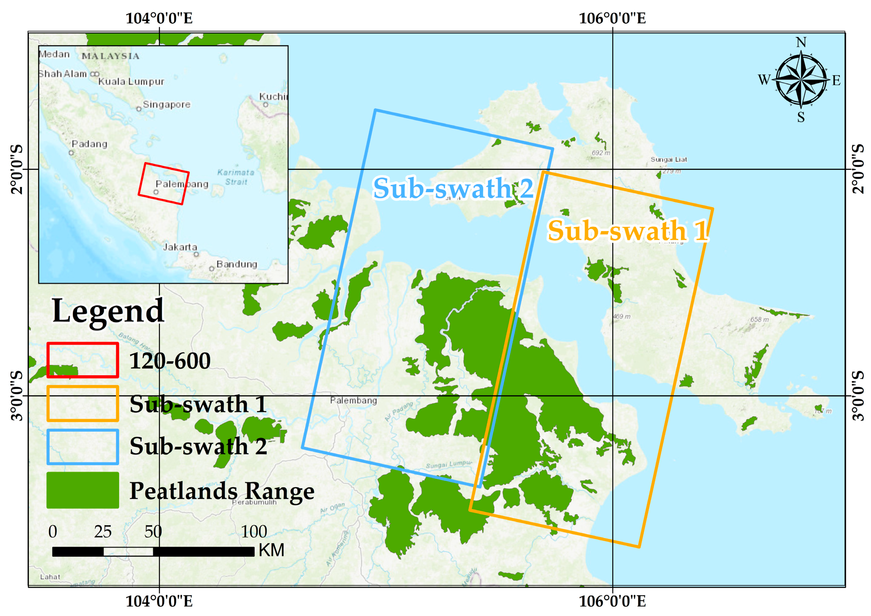
Figure 1. Location of the study area and the distribution of peatlands in South Sumatra province. Peatlands distribution is from the website of Global Peatlands.
Remotesensing 15 04461 g001
Figure 2. Distribution of four consecutive subsets in time dimension. Gray areas mean the gaps in SAR images.
Remotesensing 15 04461 g002
Figure 3. Distribution of labeled regions with high coherence in different subsets. (ad) Subsets 1, 2, 3, 4, respectively.
Remotesensing 15 04461 g003
Figure 4. Results of fitting curves of labeled regions in four subsets.
Remotesensing 15 04461 g004
Figure 5. An example of the continuous coherence 3D model with a 12-day time threshold. Pixels with high coherence are colored yellow, and those with low coherence are colored blue. The horizontal axis represents the time series, and the model’s flank is composed of range direction and azimuth direction.
Remotesensing 15 04461 g005
Figure 6. An example of the construction of adaptive HCTSs.  N 0  means the minimum number of SAR images in a temporal subset.  N i  represents the number of pixels with high coherence in the current temporal subset.  S t  is the step length between the temporal subsets.
Remotesensing 15 04461 g006
Figure 7. Example of the adaptive HCTSs’ distribution in the whole time series. Blue squares represent the start time, green squares mean the end time and the red lines are the duration of TCSs. The horizontal axis means time dimension, and the black line segments are temporal subsets.
Remotesensing 15 04461 g007
Figure 8. Flowchart of the adaptive HCTSs SBAS-InSAR processing.
Remotesensing 15 04461 g008
Figure 9. Deformation results of peatlands in South Sumatra province based on adaptive HCTSs SBAS-InSAR. (a) Average deformation rate of study region in the whole time series. (b) Average deformation rate of study region in 2019. (c) Average deformation rate of study region in 2020. (d) Average deformation rate of study region in 2021. (e) Average deformation rate of study region in 2022.
Remotesensing 15 04461 g009
Figure 10. Spatial distribution of fire hotspots in South Sumatra province (2019–2022) provided by MODIS.
Remotesensing 15 04461 g010
Figure 11. Maps of deformation results and the value of NDVI in the region with a relatively high deformation rate. (a) Average deformation results in the whole time series. (be) Average deformation results of the focused region from 2019 to 2022. (fj) Maps of the value of NDVI in the focused region at different times (10 March 2019, 13 April 2020, 16 October 2020, 19 October 2021, 11 April 2022). (A–E) Five parts of the region that showed high deformation rate in the deformation result of 2022.
Remotesensing 15 04461 g011
Figure 12. Results of reliability validation of the peatland’s deformation results. (a) Map of overlapping area between two sub-swaths. (b) Correlation results between two sub-swaths based on the deformation results in 2019. (c) Correlation results between two sub-swaths based on the deformation results in 2020. (d) Correlation results between two sub-swaths based on the deformation results in 2021. (e) Correlation results between two sub-swaths based on the deformation results in 2022. (f) Correlation results between two sub-swaths based on the deformation results in the whole time series (2019–2022).
Remotesensing 15 04461 g012
Figure 13. Deformation results of comparative SBAS-InSAR experiments in South Sumatra province. (A) Average deformation rate of study region in 2019. (B) Average deformation rate of study region in 2020. (C) Average deformation rate of study region in 2021. (D) Average deformation rate of study region in 2022. (E) Average deformation rate of study region during 2019–2022 (Whole 1). (F) Average deformation rate of study region during 2019–2022 by using time-weight method (Whole 2). (ad) Land use features of the four regions in optical remote sensing images provided by Google Earth Image.
Remotesensing 15 04461 g013
Figure 14. (a) Improvement of the number of measurement points between experiments with the proposed method and comparative SBAS-InSAR experiments. (b) Improvement of the coverage area of measurement points between experiments with the proposed method and comparative SBAS-InSAR experiments.
Remotesensing 15 04461 g014
Table 1. Sentinel-1 SAR data in this experiment.
YearPath-FrameTime RangeNumber of SAR ImagesOrbit Direction
2019120-6008 January 2019–22 December 201923Descending
2020120-6003 January 2020–28 December 202024Descending
2021120-6009 January 2021–23 December 202122Descending
2022120-6004 January 2022–30 December 202221Descending
Table 2. Landsat data in this experiment.
NumberPath-RowData Acquisition TimeSensor
1123-06210 March 2019Landsat 8
2123-06213 April 2020Landsat 8
3123-0626 October 2020Landsat 8
4123-0629 October 2021 Landsat 8
5123-06211 April 2022Landsat 9
Table 3. Detailed information on four subsets.
Master ImageTime RangeNumber of SAR Images
Subset 112 August 20192 August 2019–27 January 202015
Subset 26 August 20206 August 2020–27 April 202123
Subset 313 August 202113 August 2021–4 May 202213
Subset 49 January 20219 January 2021–27 April 202110
Table 4. Fitting results of the labeled regions in four subsets.
Subset 1Subset 2
  γ 0   γ   τ   γ 0   γ   τ
Region 10.54090.079419.9547Region 10.46830.08118.006
Region 20.51090.087313.3393Region 20.49610.081716.8464
Region 30.61690.082823.0578Region 30.45890.08116.1096
Region 40.66240.086216.9992Region 40.35990.078730.9161
Region 50.63230.082514.4918Region 50.39520.082328.2754
Average0.592680.0836417.56856Average0.435680.0809422.0307
Subset 3Subset 4
  γ 0   γ   τ   γ 0   γ   τ
Region 10.55340.088410.4404Region 10.6760.068923.1483
Region 20.51450.08439.6184Region 20.58540.080423.181
Region 30.66450.084517.2163Region 30.58850.078726.3481
Region 40.5560.084325.1663Region 40.59860.070523.5385
Region 50.42240.089317.6846Region 50.51060.068926.1949
Average0.542160.0861616.0252Average0.591820.0734824.48216
Table 5. Results of HCTSs in Sub-swath 1 and Sub-swath 2.
Sub-Swath 1Sub-Swath 2
No.Time RangeMaster
Image
Number of Images
(Inter 1)
Time RangeMaster ImageNumber of Images
(Inter 1)
18 January 2019–1 June 20199 March 201911 (15)8 January 2019–1 June 20199 March 201911 (15)
22 August 2019–3 January 202023 October 201913 (23)2 August 2019–3 January 202023 October 201913 (23)
35 September 2019–27 January 202016 November 201913 (23)5 September 2019–27 January 202016 November 201913 (23)
43 March 2020–19 June 20208 April 20208 (10)3 March 2020–19 June 20208 April 20208 (10)
56 August 2020–21 January 202117 October 202015 (27)6 August 2020–26 February 202129 October 202018 (33)
630 August 2020–2 February 202110 November 202014 (25)30 August 2020–10 March 20214 December 202017 (31)
723 September 2020–26 February 20214 December 202014 (25)23 September 2020–22 March 202116 December 202016 (29)
817 October 2020–22 March 202128 December 202014 (25)17 October 2021–15 April 20219 January 202116 (29)
910 November 2020–3 April 20219 Januray 202113 (23)10 November 2020–21 May 20212 February 202116 (28)
104 December 2020–21 May 202114 February 202114 (24)13 August 2021–17 March 20225 November 202116 (24)
1113 August 2021–9 February 202224 October 202114 (22)6 September 2021–29 March 202211 December 202115 (22)
126 September 2021–5 March 202217 November 202113 (19)30 September 2021–10 April 202223 December 202114 (20)
1330 September 2021–10 April 202223 December 202114 (20)24 October 2021–4 May 202216 January 202214 (20)
1424 October 2021–4 May 202216 Januray 202214 (20)8 August 2022–30 December 20227 October 202212 (15)
158 August 2022–30 December 20227 October 202212 (15)
1 Inter means the number of interferograms.
Table 6. Details about the reference points.
Reference PointsSub-SwathLocation (Longitude, Latitude)Land Use
  P 1 1(105°58′25.19″E, 3°18′4.92″S)Urban
  P 2 2(104°42′00.00″E, 2°54′7.02″S)Urban (near to the GPS Station)
Table 7. Detailed deformation results of peatlands in South Sumatra province from 2019 to 2022.
Min Subsidence Rate (mm/year)Max Uplift Rate (mm/year)
2019−390283
2020−324436
2021−398260
2022−735327
Whole−567347
Table 8. Statistics of comparative information between comparative SBAS-InSAR experiments and experiments based on the adaptive HCTSs SBAS-InSAR.
Number and coverage percent of measurement points in the comparative SBAS-InSAR experiments
2019202020212022Whole 1Whole 2
Sub-swath 1 (Points Number)38,22139,19540,08029,1225172104,908
Sub-swath 2 (Points Number)186,475184892195,595209,057124,467303,075
Coverage Percent in Sub-swath 1 (%)2.42.42.51.80.36.6
Coverage Percent in Sub-swath 2 (%)4.44.34.64.92.97.1
Number and coverage percent of measurement points in experiments based on the adaptive HCTSs SBAS-InSAR
2019202020212022Whole
Sub-swath 1 (Points Number)211,539479,287362,905216,792659,378
Sub-swath 2 (Points Number)542,354561,776416,772434,282773,624
Coverage Percent in Sub-swath 1 (%)13.430.423.113.841.9
Coverage Percent in Sub-swath 2 (%)12.913.39.910.218.3
Improvement of the number of measurement points (times)
Sub-swath 1 5.512.29.17.4127.46.2
Sub-swath 22.932.12.16.22.5
Disclaimer/Publisher’s Note: The statements, opinions and data contained in all publications are solely those of the individual author(s) and contributor(s) and not of MDPI and/or the editor(s). MDPI and/or the editor(s) disclaim responsibility for any injury to people or property resulting from any ideas, methods, instructions or products referred to in the content.