A Downscaling Method Based on MODIS Product for Hourly ERA5 Reanalysis of Land Surface Temperature

Abstract

Land surface temperature (LST) is a critical parameter for the dynamic simulation of land surface processes and for analyzing variations on regional or global scales. Obtaining LST with high spatiotemporal resolution is a subject of intensive and ongoing research. This study proposes a pixel-wise temporal alignment iterative linear regression model for downscaling based on MODIS LST products. This approach allows us to address the problem of high temporal resolution but low spatial resolution of the ERA5 reanalysis LST product while remaining immune to the pixel loss caused by clouds. The hourly ERA5 LST of the study area for 2012–2021 was downscaled to a 1000 m resolution, and its accuracy was verified by comparison with measured data from meteorological stations. The downscaled LST offers intricate details and is faithful to the LST characteristics of distinct land-cover categories. In comparison with other downscaling techniques, the proposed technique is more stable and preserves the spatial distribution of the ERA5 LST with minimal missing pixels. The pixel-wise average R² and mean absolute error for the MODIS view times are 0.87 and 2.7 K, respectively, for cloud-free conditions on a 1000 m scale. The accuracy verification using data from meteorological stations indicates that the overall error is lower during cloudless periods rather than during overcast periods, during the night rather than during the day, and at MODIS view times rather than at non-view times. The maximum and minimum mean errors are 0.13 K for cloud-free periods and −0.98 K for cloudy periods, indicating a slight underestimation and overestimation, respectively. Conversely, the maximum and minimum mean absolute errors are 2.01 K for the daytime and 0.85 K for the nighttime. Therefore, the model ensures higher accuracy during cloudy periods with only the clear-sky LST used as input data, making it suitable for long-term, all-weather ERA5 LST downscaling.

1. Introduction

In recent years, land surface temperature (LST) has become one of the most critical environmental covariates in scientific research [1]. It plays an essential role in various fields, such as urban remote sensing [2,3], vegetation analysis [4], and cryosphere remote sensing [5]. Using only conventional fixed-point observation on the ground makes obtaining the continuous spatial and temporal distributions of LST difficult, leaving satellite remote sensing as the only feasible means of data acquisition [6]. Remote sensing techniques, such as thermal infrared and microwave techniques, can be used to capture LSTs. However, microwave sensors typically have lower spatial resolution to acquire LSTs. The spatial and temporal resolutions of thermal infrared LST detectors are mutually constrained, and the weather often prevents complete data from being acquired. For instance, the MODIS sensor can acquire a spatially continuous LST under cloud-free conditions; however, the temporal continuity of LST is limited by the satellite revisit interval and cloud coverage.

Research has shown that over 60% of the MODIS data in mid-latitude regions are affected by weather, with clouds being the main culprit [7]. Compared with remote sensing data, reanalysis data can offer spatiotemporally continuous surface-temperature information. For example, the ERA5 reanalysis LST product from the European Centre for Medium-Range Weather Forecasts provides a global hourly LST, albeit at a spatial resolution of only 0.1°. To satisfy the demand for a LST with high spatiotemporal resolution, spatial downscaling of high temporal resolution LST has become an active research area in recent years [8,9]. The goal of such research is to improve the spatial resolution of a downscaled LST.

Currently, LST downscaling methods can be broadly classified into two categories. The first category is based on image fusion, which involves fusing low spatial resolution and high temporal resolution LST data with high spatial resolution and low temporal resolution LST data to obtain high spatiotemporal resolution LST data [10,11]. Examples of such methods include the spatial and temporal adaptive reflectance fusion model (STARFM) [12], the enhanced STARFM (ESTARFM) [13], the spatiotemporal adaptive data fusion algorithm for temperature mapping [10], the spatiotemporal integrated temperature fusion model [11], and the deep-learning-based spatiotemporal temperature fusion network [14]. These models all use MODIS LST data fusion technology and require only minimal auxiliary data while still maintaining good spatial texture for downscaled LST data. However, downscaled LST methods using image fusion techniques often overlook the radiative transfer of thermal infrared remote-sensing information [15] and, therefore, lack clear physical mechanisms and scientific significance. Thus, to ensure the energy balance of surface thermal radiation information before and after downscaled LST, statistical regression downscaling methods based on the “scale-invariant relationship” hypothesis have emerged.

The second type of method for downscaling LST may be broadly classified as statistical regression based on scale factors. The principle of such methods is to establish a statistical regression relationship between the LST and single or multiple land surface parameters and to assume that this statistical relationship is independent of spatial scales. Vegetation indices are the most used input parameters in statistical regression methods. For example, the DisTrad algorithm [16] downscales LST by establishing a linear regression between the LST and normalized difference vegetation index (NDVI). The TsHARP algorithm [17] downscales the MODIS 1 km LST to 250 m and GOES 5 km LST to 1 km by establishing a linear relationship between the LST and vegetation cover. The HUTS algorithm [18] downscales LSTs by establishing a regression relationship between the LST and the NDVI on the one hand and surface reflectance on the other hand. In addition, geographically weighted regression methods based on the NDVI and digital elevation models have also been applied to downscaling research [19]. Machine-learning methods can handle complex nonlinear statistical regression problems and have been applied with success to downscaling remote sensing data. Previous studies have used artificial neural networks, random forests, support vector machines, and other methods combined with the NDVI, leaf area index, surface reflectance, digital elevation models, and other remote sensing indices as input parameters to downscale LST [20,21,22,23]. Previous work evaluated the use of the machine-learning methods of random forests, neural networks, and support vector machines for downscaling different land-cover types and concluded that the random forest method is more stable and accurate than the other two methods [24].

Most of these methods establish a relationship between surface temperature and various parameters based on the global scale, ignoring the local characteristics of the relationship between parameters [19]. Considering that there is significant spatial heterogeneity in the distribution of land surface temperature, and the relationship between factors will change with geographical location, some scholars have begun to study the spatial non-stationarity relationship between the land surface temperature and surface physical parameters. Geographically Weighted Regression (GWR), Geographically and Temporally Weighted Regression (GTWR) and Geographically Weighted Auto Regressive (GWAR) methods were used to improve the scaling accuracy of land surface temperature (LST) and enhance the spatial texture characteristics of the LST data after scaling [19,25].

However, most input surface parameters (e.g., NDVI, leaf area index, and FVC) for the above-mentioned LST downscaling methods are calculated from visible or near-infrared remote-sensing images, which greatly limits the applicability of the downscaling methods under cloud cover. For the all-weather acquisition of LST data, various schemes have been proposed for a cloud-free LST reconstruction based on multi-source auxiliary information, LST inversion based on microwave remote-sensing data, and LST fusion based on synergistic thermal infrared and microwave remote-sensing data [25,26,27]. However, whether these methods can be applied to the spatial downscaling of LST remains a critical issue that needs to be explored and addressed.

Given the discussion above, developing a method to downscale LST that is not limited by weather conditions and guarantees the spatial completeness and temporal continuity of the downscaled LST is an urgent problem that needs to be solved. The ERA5 reanalysis data from the European Centre for Medium-Range Weather Forecasts provides hourly LSTs with high temporal resolution, a long time span, and easy accessibility. Previous studies show that the ERA5 LST product correlates strongly with actual LSTs, although the error is non-zero. However, whether it can be downscaled spatially to increase the spatiotemporal resolution requires further research. The present study thus proposes a pixel-wise temporal alignment iterative linear regression model (PTAILRM) for downscaling the ERA5 LST product based on the MODIS LST product and air temperature factors. The method involves time matching and iterative linear regression of each pixel, downscaling the continuously time-resolved, coarse-resolution ERA5 LST to a fine resolution and temporally sampling it to local time at whole-hour intervals. In this study, the ERA5 LST in the study area was downscaled to a resolution of 1000 m using the proposed method. The downscaling results of land-cover data and other representative methods were employed for qualitative evaluation, while the site-measured data were used for quantitative evaluation.

2. Study Area and Material

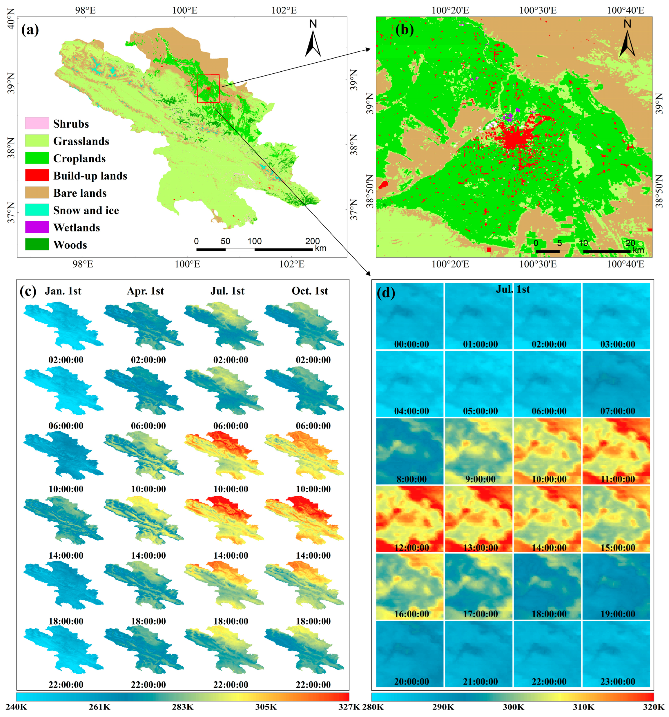
2.1. Study Area

The study area encompasses Zhangye City and Haibei Tibetan Autonomous Prefecture, located in the middle reaches of the Heihe River Basin, with a total area of approximately 73,000 square kilometers. Zhangye City is in the middle section of the Hexi Corridor and is characterized by flat terrain dominated by cropland, grassland, bare soil, and wetland. The Haibei Tibetan Autonomous Prefecture is in the central part of the Qilian Mountains, with rugged terrain and elevations ranging from 2180 to 5287 m above sea level. Areas above 3000 m account for more than 85% of the total prefectural area and are mainly covered by cropland, grassland, and bare soil. Figure 1 shows the study area’s geographical location, elevation, and land cover.

2.2. Material

(i)

The European Centre for Medium-Range Weather Forecasts provides the fifth-generation reanalysis climate dataset ERA5, which offers hourly reanalyzed data from 1979 onwards and is continuously updated. This dataset assimilates numerical weather forecasts, a significant amount of ground observation data, and satellite remote sensing information and offers a high temporal resolution and long time span. Within the research area, we selected from ERA5-Land the hourly land surface temperature (LST) and air temperature (AT) products with a spatial resolution of 0.1° to conduct a long-term, all-weather analysis of LST downscaling.

(ii)

The MOD11A1 and MYD11A1 products used in this study include daytime and nighttime surface temperature inversions from the Terra and Aqua satellites, respectively. The combined MOD11A1 and MYD11A1 products provide a sampling frequency of four times per day and are inverted by the generalized split-window algorithm to yield a surface temperature with approximately 1 km resolution [28]. In addition, the study also uses the quality control (QC) layer and imaging time layer provided in the dataset.

Table 1. MODIS LST product used in this study.

Data Layer	Units	Description
LST_Day_1 km	Kelvin	Daytime LST
LST_Night_1 km	Kelvin	Nighttime LST
Day_view_time	Hours	Local time of day observation
Night_view_time	Hours	Local time of night observation
QC_Day	-	Daytime LST Quality Indicators
QC_Night	-	Nighttime LST Quality indicators

provides the data acquisition status.

(iii)

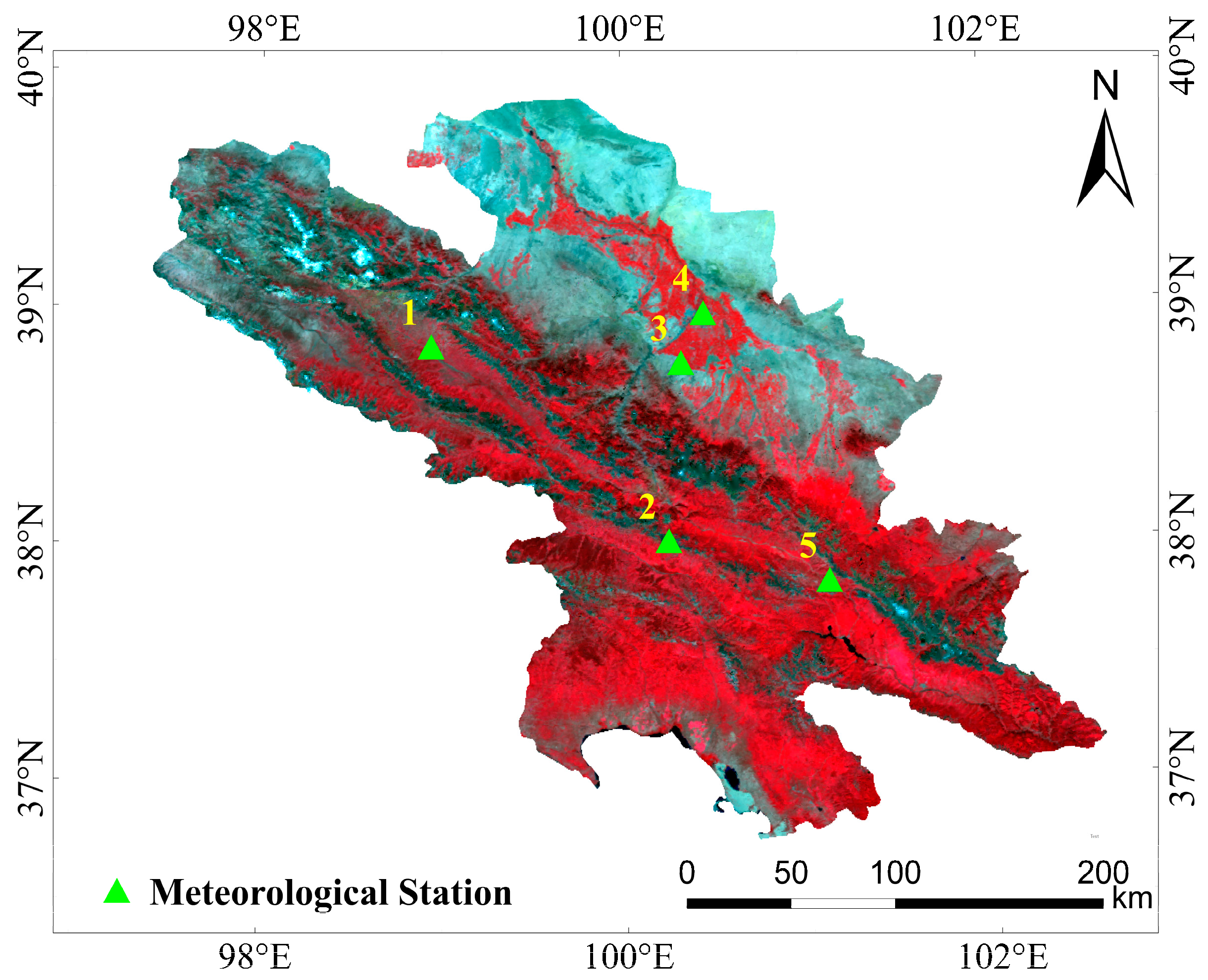
The observed meteorological data used to verify the accuracy were obtained from the National Tibetan Plateau Science Data Center. Figure 2 shows the locations of the meteorological stations within the study area, and

Table 2. Information for each meteorological station.

ID	Site Name	Altitude	Sampling Time Interval	Time Range
1	Zhangye	1460 m	10 min	1 January 2012–31 December 2021
2	Yakou	4148 m	10 min	1 January 2012–31 December 2021
3	Jingyangling	3750 m	10 min	1 January 2012–31 December 2021
4	Huazhaizi	1731 m	10 min	1 January 2012–31 December 2021
5	Dashalong	3739 m	10 min	1 January 2012–31 December 2021

provides information on the altitude and time range for each station. The observation dataset is the up-and-down longwave radiation recorded every 10 min by the meteorological stations [29]. The observed surface temperature was calculated as follows by applying the Stefan–Boltzmann law to the up-and-down longwave radiation and MODIS emissivity dataset:

$$T_s={\left(\frac{L_{\uparrow }-\left(1-{\epsilon }_b\right)L_{\downarrow }}{{\epsilon }_b\sigma }\right)}^{1/4},$$

(1)

$${\mathsf{\epsilon }}_{\mathrm{b}}=0{.2122\mathsf{\epsilon }}_{29}+0{.3859\mathsf{\epsilon }}_{31}+0{.4029\mathsf{\epsilon }}_{32}$$

(2)

In Equation (1), L_↑ and L_↓ are the up and down longwave radiation, respectively, and σ is the Stefan–Boltzmann constant [5.67 × 10⁻⁸ [W/(m²·K⁴)]]. The broadband emissivity ε_b is calculated according to Equation (2) by using the MODIS land surface emissivity dataset [30], where ε₂₉, ε₃₀, and ε₃₁ are the narrowband emissivities of MODIS bands 29, 30, and 31, respectively.

3. Methodology

3.1. The PTAILRM Downscaling Method

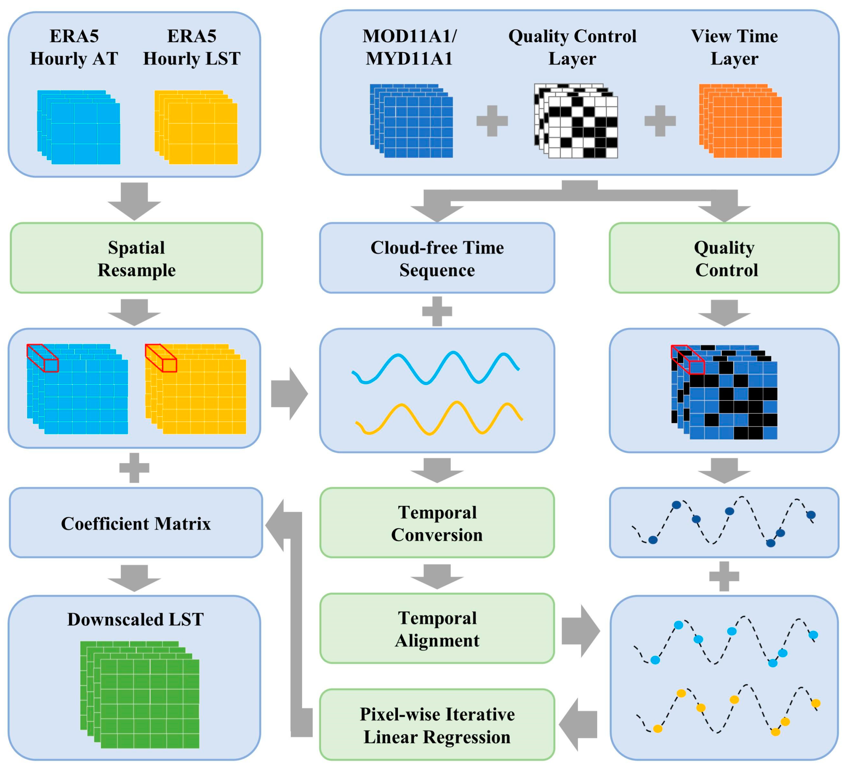
3.1.1. Overview of PTAILRM

The PTAILRM downscaling method primarily consists of four components. Step 1: Preprocessing of the ERA5 data and MODIS LST product, which involves spatial resampling of the ERA5 data and quality control of the MODIS LST product. Step 2: Temporal alignment of the ERA5 data at each pixel, including converting each pixel’s Greenwich time to local time and interpolating the ERA5 product to match the transit time of the MODIS sensor. Step 3: Pixel-wise iterative linear regression using the time series of the ERA5 LST and AT as independent variables and the time series of the MODIS LST at a higher spatial resolution as the dependent variable. This step primarily involves establishing a linear regression model for each datum and iteratively determining the optimal time offset to obtain the regression coefficient matrix. Step 4: Downsampling of the ERA5 LST and AT based on the coefficient matrix, followed by raster calculations to obtain downscaled LSTs. See Figure 3 for a detailed description of the process.

3.1.2. Preprocessing of ERA5 and MODIS LST Products

The ERA5 hourly raster data for the LST and AT was resampled through bilinear interpolation to achieve a 1000 m resolution that aligns with the MODIS LST products. Although this process did not amplify the amount of information, empirical evidence shows that, compared with the nearest-neighbor interpolation method, this process mitigates the impact of significant gradient fluctuations at the edges of low-resolution pixels on the downscaling. The QC layer of the MOD11A1 and MYD11A1 LST products is used to mask the cloud-affected areas, preserving high-quality pixels with an average LST and emissivity errors of less than 1 K and 0.01, respectively, by eliminating non-zero pixels. This requires the use of the QC_Day and QC_Night data layers of byte types specified in Table 1 and the corresponding bit mask information provided in

Table 3. Bitmask description for QC_Day and QC_Night layers.

Bits Location	Value	Description	Flag Name
Bits 0 and 1	0	LST produced, good quality, not necessary to examine more detailed QA	Mandatory QA flags
	1	LST produced, other quality, recommend examination of more detailed QA
	2	LST not produced due to cloud effects
	3	LST is not produced primarily due to reasons other than cloud
Bits 2 and 3	0	Good data quality	Data quality flag
	1	Other quality data
	2	TBD
	3	TBD
Bits 4 and 5	0	Average emissivity error ≤ 0.01	Emissivity error flag
	1	Average emissivity error ≤ 0.02
	2	Average emissivity error ≤ 0.04
	3	Average emissivity error > 0.04
Bits 6 and 7	0	Average LST error ≤ 1 K	LST error flag
	1	Average LST error ≤ 2 K
	2	Average LST error ≤ 3 K
	3	Average LST error > 3 K

. The ERA5 AT, LST, and MODIS LST data units were eventually converted to Kelvin.

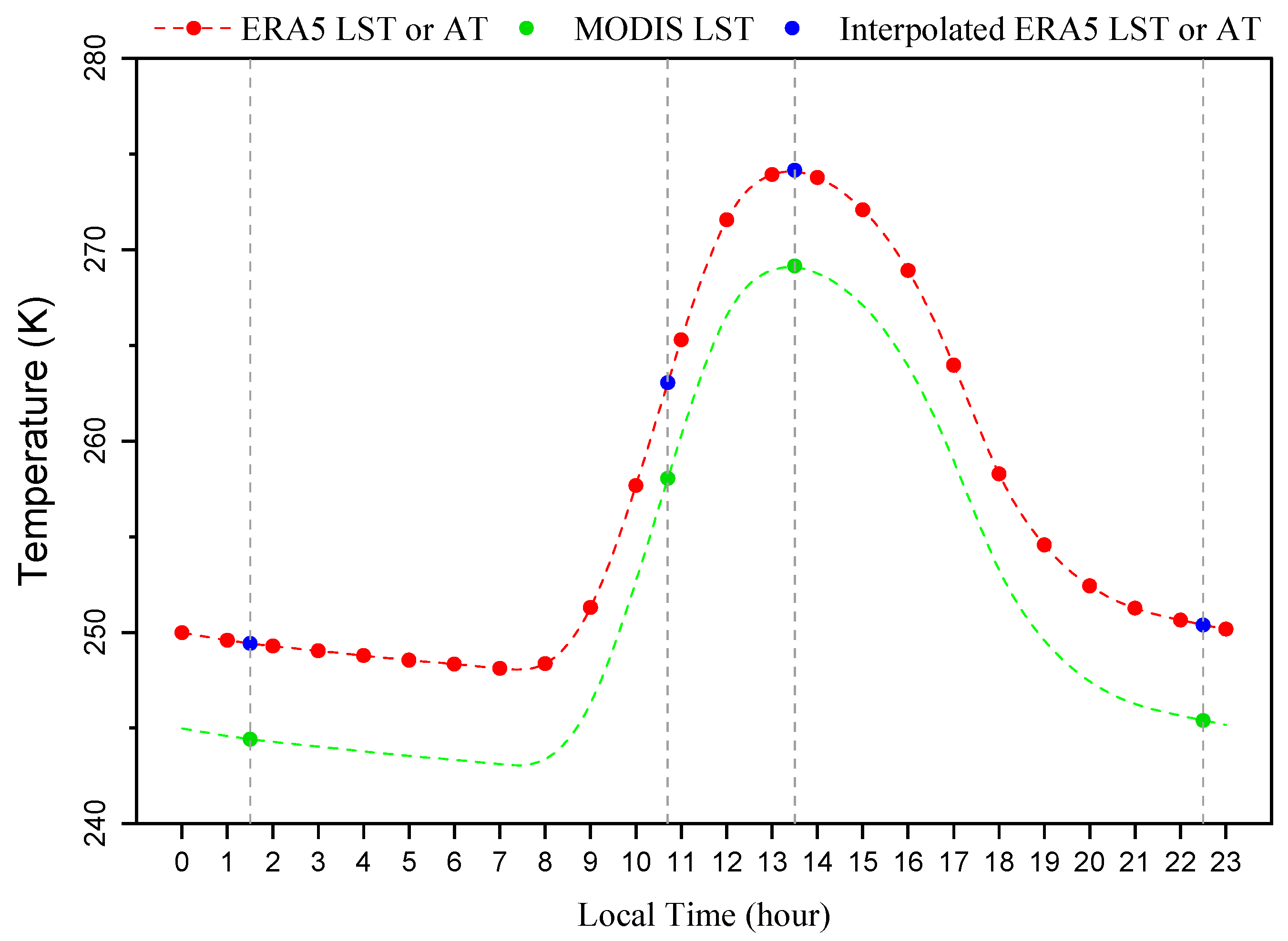
3.1.3. Pixel-Wise Temporal Conversion and Alignment

The ERA5 reanalysis data product is provided in Greenwich Mean Time, whereas the MODIS LST product is provided in local time. Due to the scanning characteristics of the MODIS instrument, variations exist in the local solar time of a given pixel on different revisit days [31]. Figure 4 shows the local times corresponding to each MODIS overpass in the study area for 2012–2021, which are concentrated in four time periods (in decimal hours): 0.1–3, 9.9–11.9, 12.2–14.1, and 21.0–23.3. The above data are obtained from the ‘Day_view_time’ and ‘Night_view_time’ data layers in the MODIS LST product.

The LST correlates closely with the amount of solar radiation received on the ground, which in turn relates closely to the solar altitude, which varies with local time. Therefore, at the pixel scale, this study converts Greenwich Mean Time to local time, which is more closely related to the changes in surface temperature than regional time. The time conversion formula is as follows:

$$t_{il}=t_{ig}+\frac{lo{n}_i}{{15}^{°}}$$

(3)

where $t_{il}$, $t_{ig}$, and $lo{n}_i$ are the local time, Greenwich Mean Time, and longitude of pixel i, respectively, with the time measured in decimal hours.

After the time conversion at the pixel level, we temporally align the ERA5 and MODIS products because the ERA5 hourly products are provided at hourly intervals, whereas the MODIS products have irregular sampling times. Aligning the two products temporally effectively minimizes the errors caused by temporal inconsistencies, which are critical for maintaining the accuracy and reliability of the analysis.

If the function describing the LST as a function of time is continuous and differentiable everywhere, interpolation methods can be used to obtain data at a given moment in a local time frame. The cubic spline function is commonly used for processing satellite time series data. Its primary advantages include continuous first- and second-derivatives, simplicity, stability, and high accuracy in calculations [32,33,34,35].

To address the problem of inconsistent sampling times between the ERA5 and MODIS LSTs, the high and continuous temporal resolution of the ERA5 product is used in combination with the view time data layer of the MODIS product to perform a cubic spline interpolation on a pixel-by-pixel basis. This temporally aligns the two products in the time domain (as illustrated in Figure 5).

3.1.4. Establishing the Pixel-Wise Iterative Linear Regression Model

As the periodic variation in solar radiation is the leading cause of the variations in LST, the temporal patterns of LST for various land-cover types can be considered approximately synchronous. Given this, we hypothesize that the relationship between the coarse-resolution LST and fine-resolution LST for the same pixel after spatial and temporal registration is linear and remains stable within a specific time period, as expressed by the following formula:

$$F_i(t)=a_{si}+b_{si}\times C_{si}(t+t_{si})+{\epsilon }_{si}(t)$$

(4)

In Equation (4), the subscript i signifies the pixel location, the independent variable $t$ is the local time, $a_i$ and $b_i$ are the regression coefficients, $F_i$ and $C_{si}$ are the fine-resolution and coarse-resolution LSTs, respectively, and ${\epsilon }_{si}$ is the residual. Notably, a time offset parameter $t_{si}$ is introduced in the equation to mitigate errors arising from asynchronous temperature changes between $F_i$ and $C_i$. It is evident that $t_{si}$ is relatively small and fluctuates around zero, and its value varies depending on the location of pixel i.

Given that the value selected for $t_{si}$ should not be large, an iterative regression can be done with a given step size within a time window centered at zero to determine the $t_{si}$ that corresponds to the regression with the highest R². Assume the relationship between $t_{si}$ and R² is expressed by

$$R^2{}_{si}=f \left({\tau }_{si}\right); {\tau }_{si}\in \left[-\omega /2, \omega /2\right],$$

(5)

$$t_{si}=f^{-1}\left[ max\left(R^2{}_{si}\right)\right]$$

(6)

where ω is the window size, ${\tau }_{si}$ is the value of $t_{si}$ in the time window, and $R_{si}^2$ is the R² corresponding to ${\tau }_{si}$. By taking specific steps to vary $t_{si}$ within the given time window and performing iterative regression, $t_{si}$ can be determined by finding the maximum $R_{si}^2$, as given by Equation (6). Furthermore, the land and atmospheric interactions, along with energy exchange, significantly affect the LST and result in a strong correlation between the LST and AT [36,37,38]. To further improve the precision of the downscaling process, we introduce an AT factor and establish the following linear relationship between coarse-resolution AT and fine-resolution LST:

$$F_i(t)=a_{ai}+b_{ai}\times C_{ai}(t+t_{ai})+{\epsilon }_{ai}(t)$$

(7)

Equation (7) is like Equation (4) and uses the subscript i to indicate the pixel location, along with an independent variable t and the regression coefficients $a_{ai}$ and $b_{ai}$. Additionally, Equation (7) includes fine-resolution LST ($F_i$) and coarse-resolution AT ($C_{ai}$) as well as residual ${\epsilon }_{ai}$ and time offset $t_{ai}$, which can be acquired in the same way as is done for $t_{si}$.

In accordance with Equations (4) and (7), the fine-resolution LST is

$$F_i(t)=a_i+b_i\times C_{si}(t+t_{si})+c_i\times C_{ai}(t+t_{ai})+{\epsilon }_i(t)$$

(8)

and the simulated fine-resolution LST is

$${\widehat{F}}_i(t)=a_i+b_i\times C_{si}(t+t_{si})+c_i\times C_{ai}(t+t_{ai})$$

(9)

In Equations (8) and (9), the regression coefficients are $a_i$, $b_i$, and $c_i$; the residual is ${\epsilon }_i$; and ${\widehat{F}}_i$ is the simulated fine-resolution LST. The other variables have already been introduced.

Equation (9) is a relatively simple model comprising only three unknown parameters, $a_i$, $b_i$, and $c_i$, which can be determined via linear regression. The $t_{si}$ and $t_{ai}$ can be obtained through iterative regression, with a time window ω of one hour used herein. In practical downscaling operations, $t$ is expressed in cumulative decimal hours—a unit also employed in the view time layer of MODIS LST products—and its values are determined by the cloud-free imaging time series of MODIS LST products within a specific time period, which is one month in this study, ensuring sufficient data for regression analysis.

Upon iteratively performing linear regression to determine the parameter matrix, it can be combined with the temporally and spatially aligned time series of ERA5 LST and AT for band operations, ultimately yielding the hourly LST at a spatial resolution of 1000 m. The temporal coverage extends from 1 January 2012 at 00:00:00 to 31 December 2021 at 23:00:00.

3.2. Validation Strategy

3.2.1. Strategy for Qualitative Validation

The strategy for qualitative validation primarily encompasses two aspects. First, it entails evaluating the spatiotemporal rationality of LST by presenting maps of it for representative periods and analyzing daily and seasonal LST variations in conjunction with land-cover types. Second, it involves comparisons with other representative downscaling methods.

We compare the ESTARFM [13] with the proposed PTAILRM. ESTARFM functions by initially inputting two sets of coarse-resolution and fine-resolution images from the same or neighboring time periods, followed by inputting a coarse-resolution image acquired at the target date, ultimately yielding a fine-resolution image at the target date. The merit of this fusion technique resides in its capacity to account for the spatial proximity between adjacent and target pixels, spectral discrepancies, and temporal fluctuations while augmenting the accuracy of the fusion outcomes in regions with pronounced heterogeneity.

Identifying two pairs of suitable ERA5 and MODIS LSTs is relatively easy and allows us to downscale low-resolution ERA5 LSTs acquired at any given time within a proximate time range, thereby facilitating a comparison with the downscaled results of PTAILRM.

3.2.2. Quantitative Validation Strategy

This investigation precisely evaluates the MODIS overpass instances under cloud-free conditions by using goodness-of-fit indices, namely, R² and the mean absolute error (MAE). This approach verifies only the accuracy of the downscaled LST during imaging periods when the sky is transparent, yet it can be amalgamated with land-cover classifications, digital elevation models, and cloud-free pixel count (CPC) to scrutinize how disparate surface factors affect the accuracy. The emphasis is placed on examining how spatial factors affect accuracy. The CPC value is obtained by counting the number of pixels whose value is 0 in the QC_day and QC_night data layers of the MODIS LST products in a certain period of time. Based on the information provided in Table 3, the LST pixels that meet this condition have good data quality and are not affected by cloud interference; therefore, our study takes this value as the number of clear-sky pixels in a certain period. Obviously, a higher CPC value means that more data are involved in fitting the model.

The methodology for assessing the accuracy based on data from meteorological stations is used extensively with remote sensing LST products [39,40,41,42]. This approach is constrained by the quantity of data from meteorological stations and the relatively homogeneous land-cover types surrounding these stations; however, its most important feature is the temporal resolution, which facilitates the comparison and analysis of downscaled accuracy over an entire time period without being limited by weather conditions. To avoid the influence of scale factors, data from meteorological stations must serve as a singular data source for both input and accuracy validation [43]. This method underscores the relationship between temporal factors and downscaling errors. This study thus adheres to the following principles:

(1)

Data from meteorological stations are used as a single input source for analyzing the accuracy of downscaling models. That is, the ERA5 surface temperature is downscaled separately by using the PTAILRM at the spatial scale of the infrared observatory of the five meteorological stations, which prevents the scale effects from influencing the accuracy analysis.

(2)

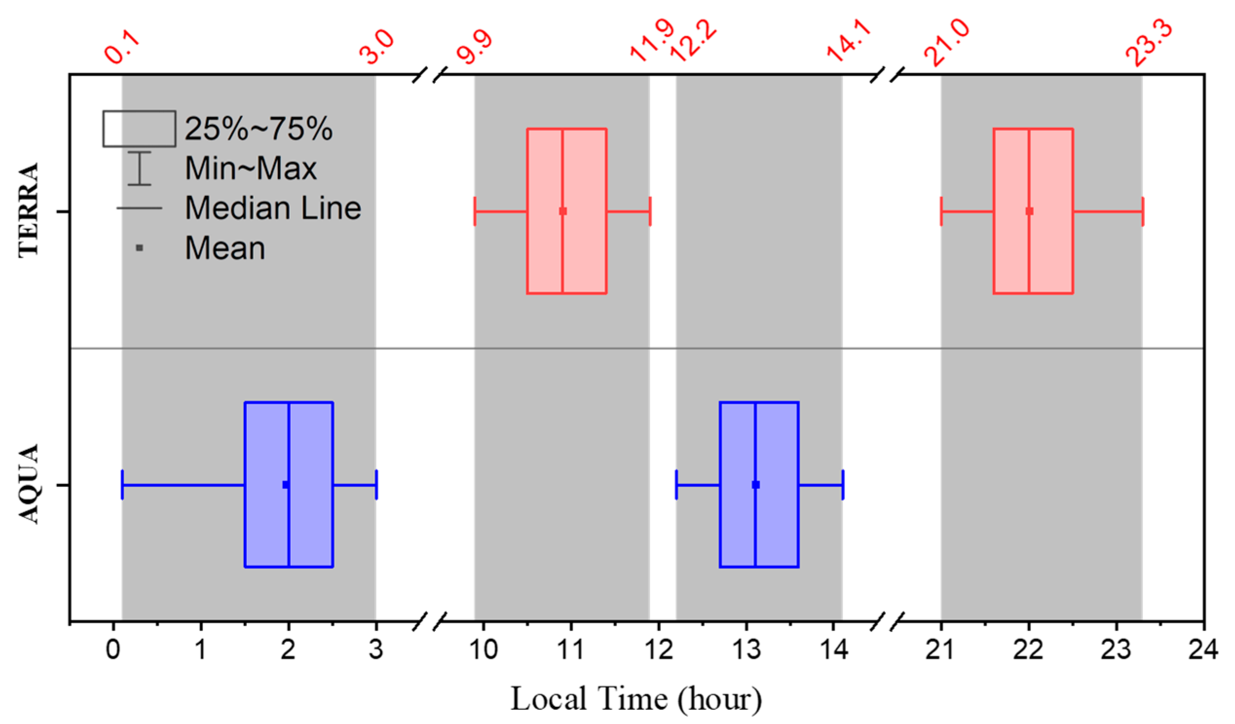
The time sampling used for the regression input data is consistent with the MODIS surface-temperature product’s clear-sky transit time on the pixel scale corresponding to each meteorological station. In other words, the sampling strategy simulates the MODIS transit time.

4. Downscaling Results

4.1. Qualitative Validation of Downscaling Results

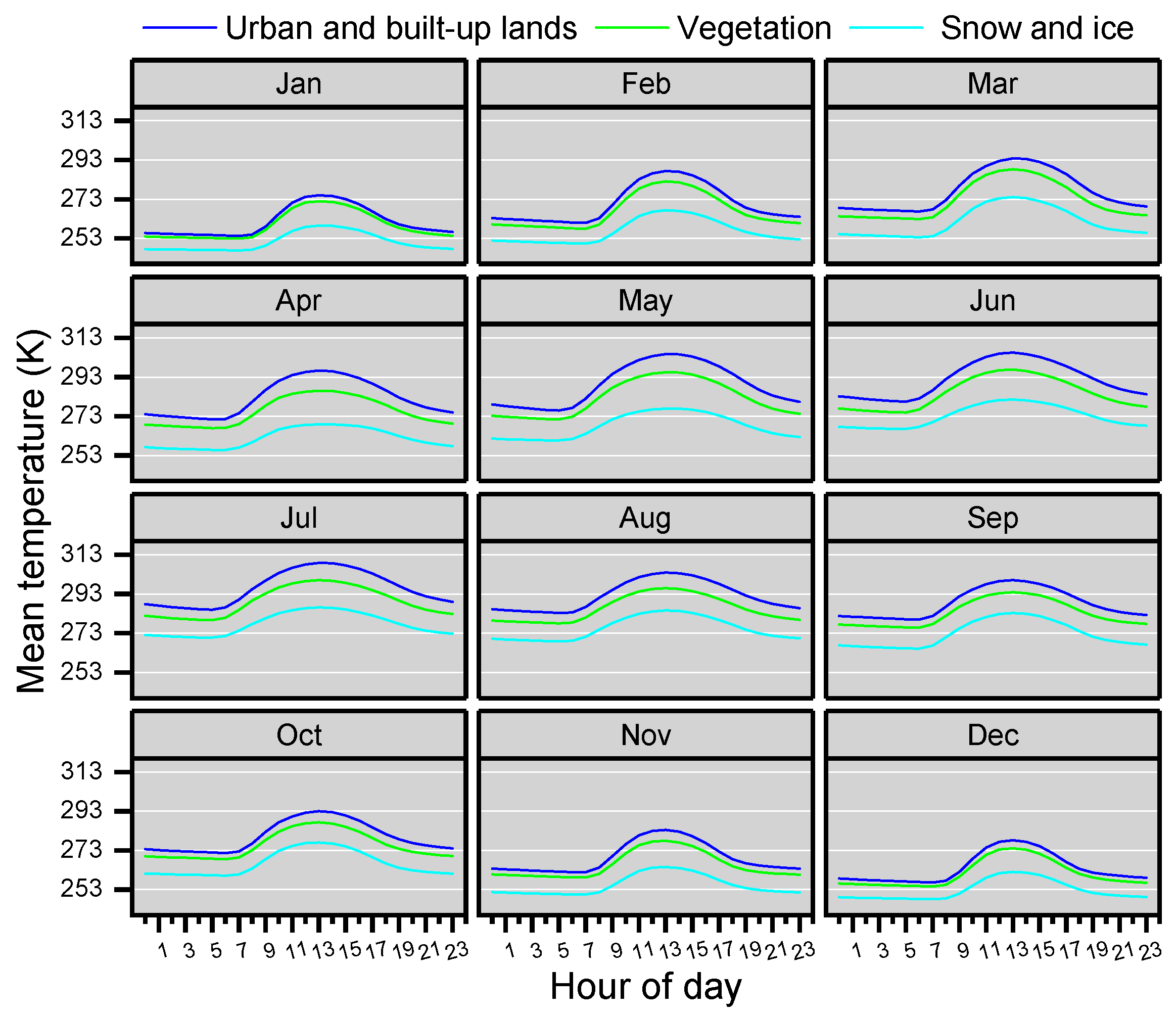
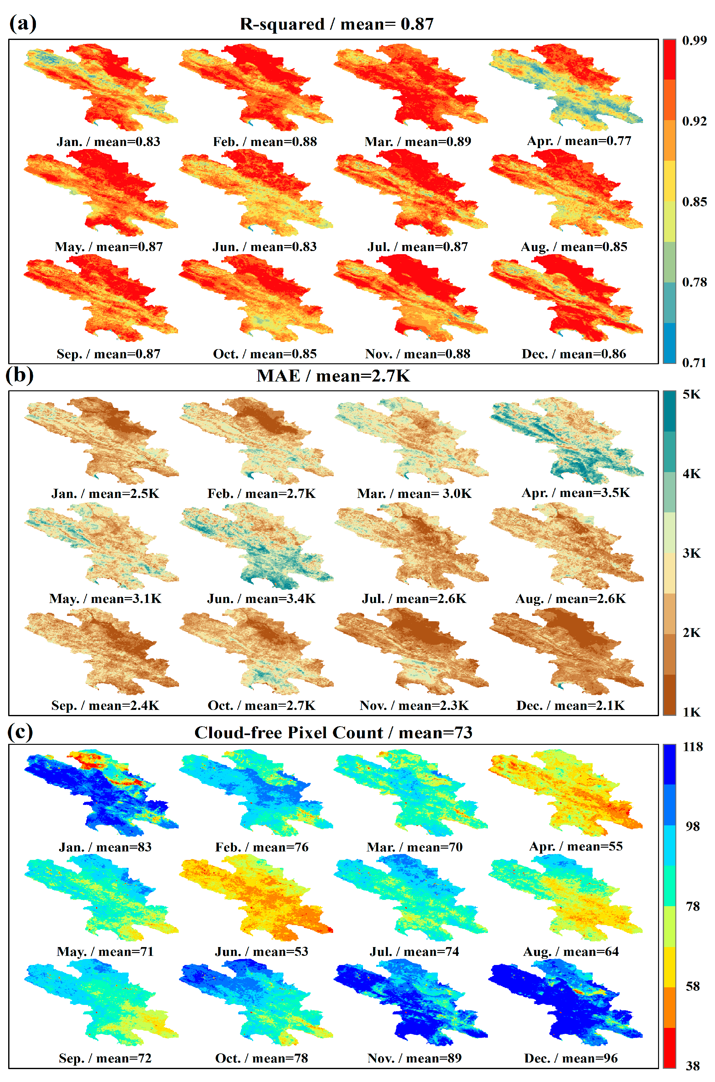
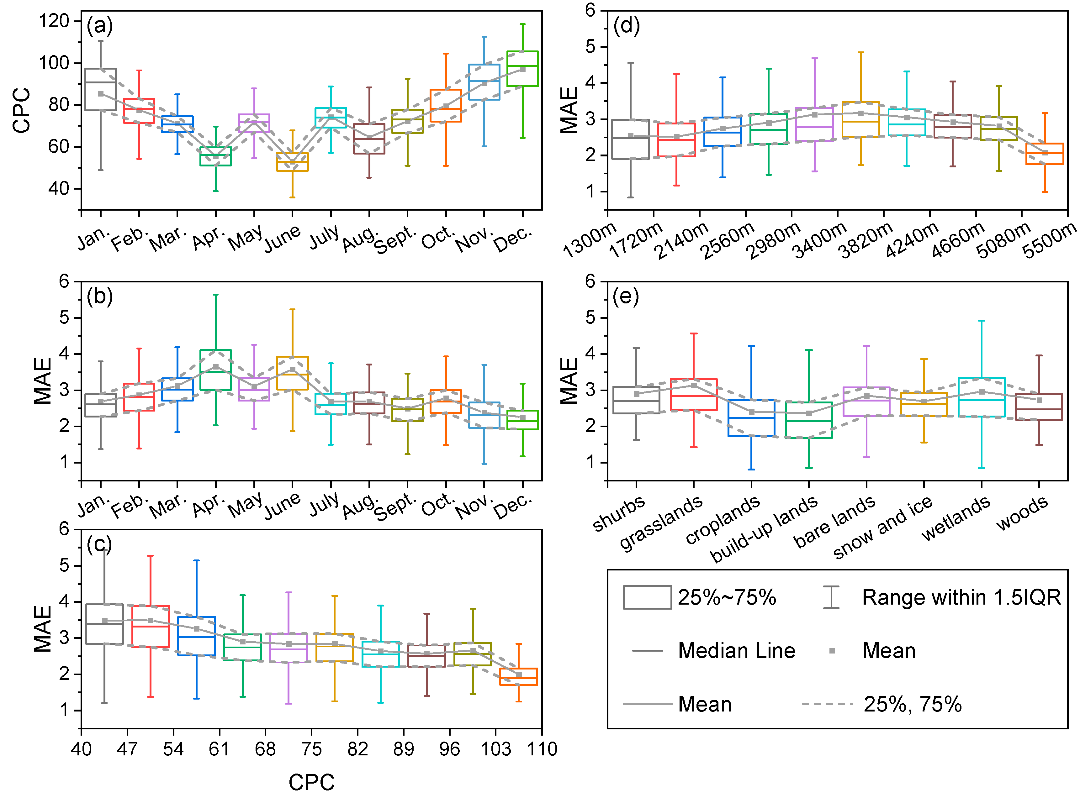
4.1.1. Validation of the Spatiotemporal Regularity of Downscaled LST

Figure 6c shows the downscaled LST on the first day of the representative months for each season in 2021. To accommodate the spatial constraints, a 4-h temporal interval was adopted. The LST derived from the PTAILRM downscaling has a rich texture, pronounced heterogeneity, superior spatial and temporal integrity, and few missing pixels. In Figure 6d, the hourly LST of the Zhangye urban area after downscaling on 1 July 2021 is shown; the LST of the urban built-up area is significantly higher than that of the surrounding cropland, showing a strong heat island effect during the day.

This study uses a monthly average method to calculate and represent the hourly diurnal variations of the downscaled LST for three distinctive surface-cover types: urban regions, vegetation, and ice- and snow-covered landscapes (see Figure 7). Correspondingly, their deviations from daily mean temperatures and daily maximum temperatures are tabulated to facilitate a comprehensive analysis and evaluation (see Figure 8).

As shown in Figure 7, the diurnal variation of the downscaled LST reveals a gradual rise in the LST within the study area from sunrise (approximately at 6:00) to its zenith around 14:00 local time. Subsequently, between 14:00 and 18:00, the LST gradually declines. Throughout the nighttime period (from 18:00 to 6:00 the following day), the temperature remains relatively low, with predictable fluctuations. In addition, it is worth noting that the temperature of urban areas is generally higher than that of vegetation, which is especially evident during the summer months.

The overall trend shown in Figure 8 suggests that the daily average temperature and the maximum temperature difference decreases in the following order: urban built-up areas, vegetation, and snow- and ice-covered areas. With regards to the downscaled LST seasonal variation pattern, the highest daily average LST occurs during summer (June–August), whereas the lowest average LST occurs during winter (December–February). During spring (March–May), the average temperature is slightly higher than during autumn (September–November).

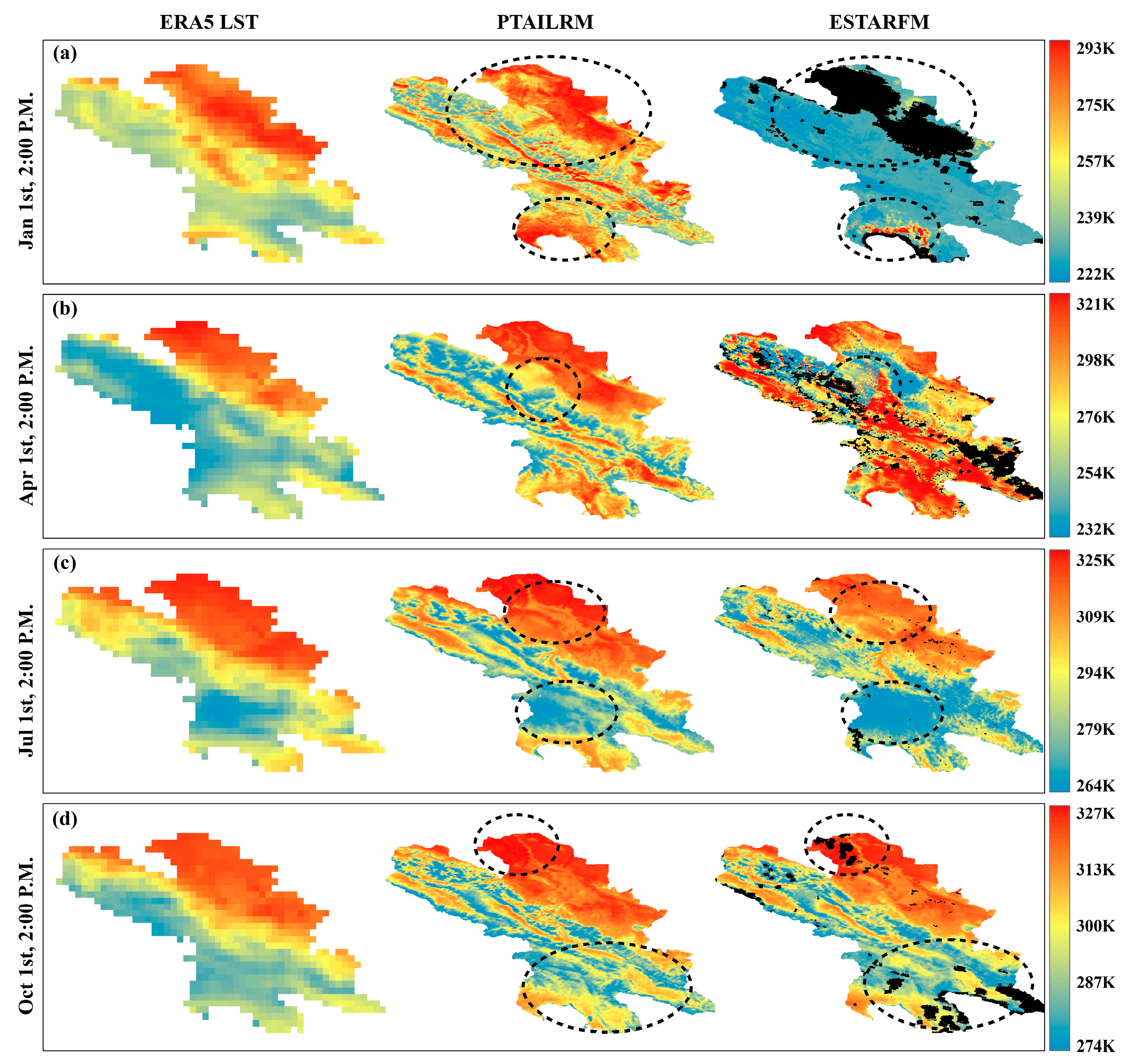
4.1.2. Comparison of PTAILRM with Alternative Downscaling Model

Figure 9 shows the original ERA5 LST at 2 p.m. on the first day of the representative months for each season and the LST downscaled by using PTAILRM and ESTARFM. The reason we selected 2 p.m. is that the LST typically reaches its daily maximum around this time and exhibits maximal spatial texture. Figure 9 shows that both downscaling models increase the spatial texture details of the LST vis-à-vis the original LST. However, the ESTARFM downscaled LST has more missing pixels than the PTAILRM downscaled LST. This phenomenon occurs at all four selected time points, especially on 1 January and 1 October. Additionally, the downscaling of ESTARFM is not stable. For 1 January, its overall temperature is lower, and the spatial distribution of the LST deviates significantly from the original LST.

Moreover, temperature anomalies occur at the lower part of the image. For 1 January, the PTAILRM downscaled LST better preserves the spatial distribution of the original LST. For April 1, ESTARFM’s downscaled image is noisy and contains serious spatial discontinuities, where the PTAILRM avoids these issues. For 1 July and 1 October, the ESTARFM downscaled results are better, with fewer missing pixels. However, the spatial texture details of the ESTARFM downscaled LST differ significantly from those of the PTAILRM in areas with high and low LSTs.

4.2. Quantitative Validation of Downscaled Results

4.2.1. Validation of MODIS Transit Times under Cloud-Free Conditions

This section analyzes the accuracy of the PTAILRM downscaling results at the monthly scale in combination with factors such as the CPC, elevation, and land-cover type.

Figure 10 shows the spatial distribution of the coefficient of determination (R²) and MAE produced by the PTAILRM and CPC. This model produces a high goodness-of-fit for each month, with the mean R² and MAE values reaching 0.87 and 2.7 K, respectively. However, the results for April and June are less precise than the other months, with R² = 0.77 and 0.83 and MAE = 3.5 and 3.4 K, respectively. Furthermore, the mean CPC values of 55 and 53 are lower during these time periods. The difference in precision between the remaining months is not significant, with the mean R² and CPC values exceeding 0.83 and 64 and the MAE values below 3.0 K.

Figure 11a–c show the statistical distribution of the MAE and CPC for each month, as well as the relationship between the distribution of the MAE data and the variation in CPCs. As the CPC increases, the fitting accuracy remains stable, whereas the uncertainty increases as the amount of data decreases.

Figure 11d,e show the statistical fluctuation of the MAE with respect to the elevation and land-cover type. The shape and pattern of the box plot indicate that the MAE varies less in terms of the elevation and land-cover type when compared to the CPC. In Figure 11d, the MAE distribution has high values in the middle elevations (around 4000 m) and low values at extreme elevations. In Figure 11d, the overall MAE for cropland and urban areas is relatively low, whereas for the grassland and wetland, it is relatively high compared with other land-cover types.

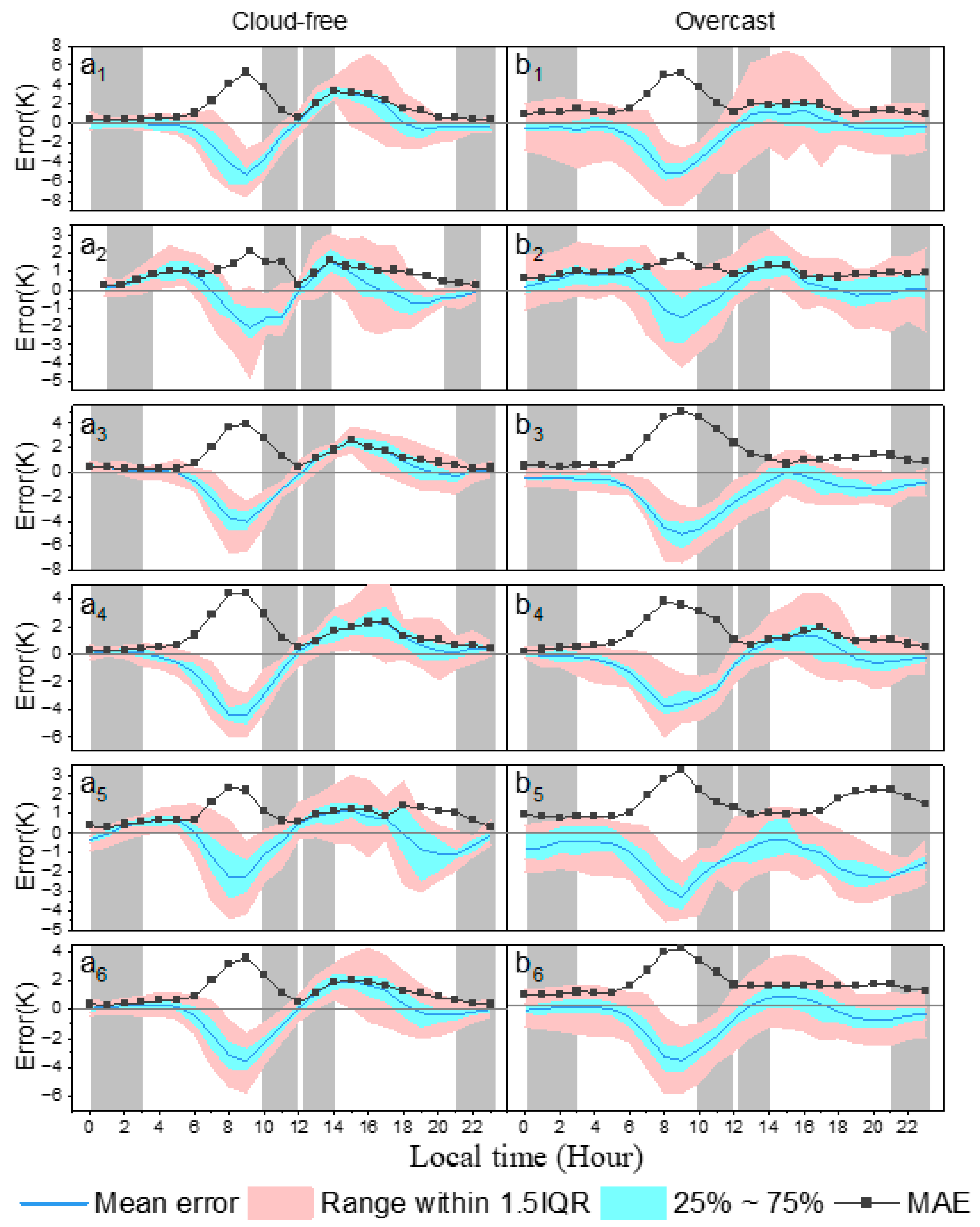
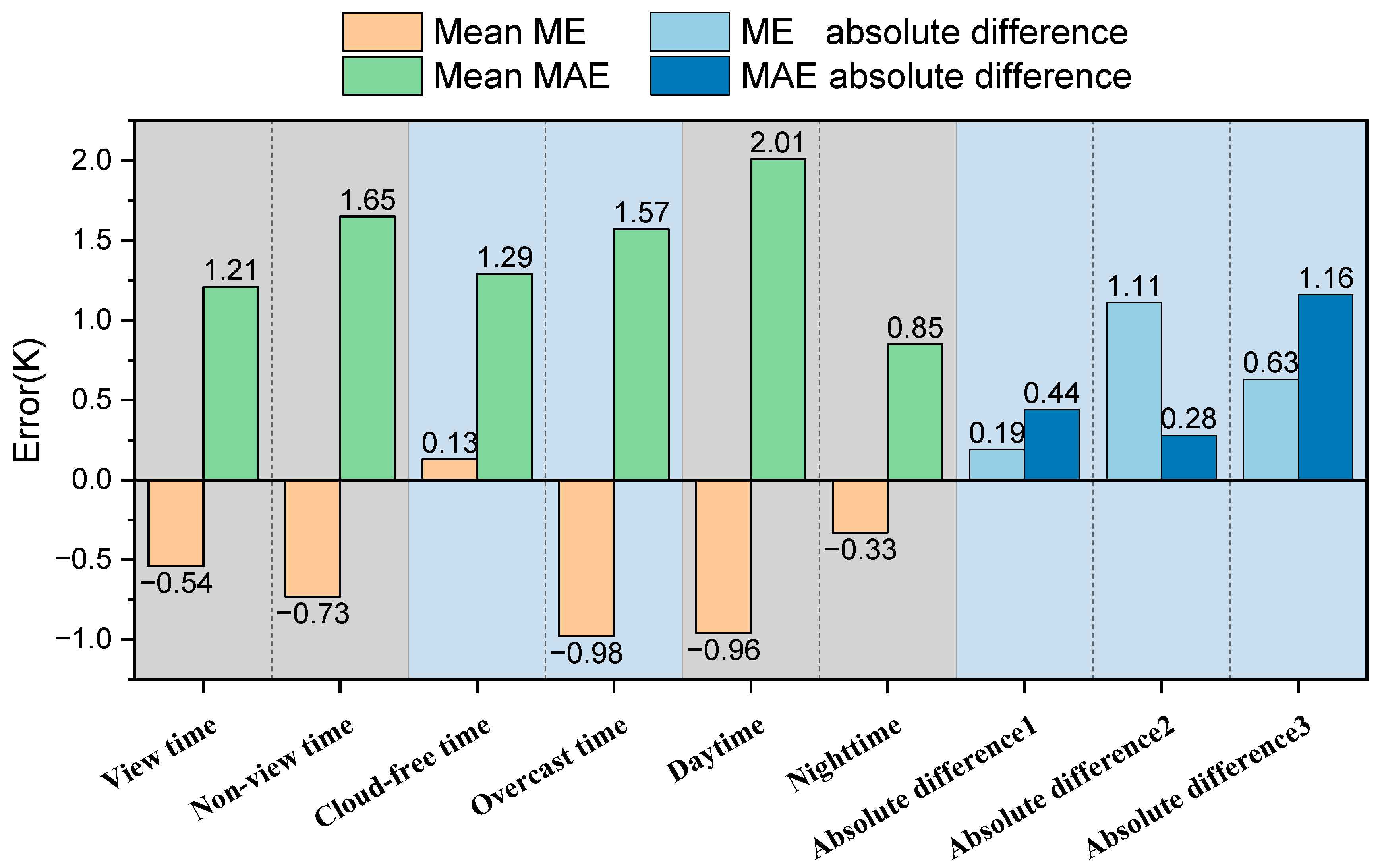
4.2.2. Validation for All Time Periods Based on Data from Meteorological Stations

Figure 12 shows the statistical distribution of the errors in the downscaled results on an hourly scale for the annual mean, using error, mean error (ME), and MAE as the evaluation metrics. Figure 12(a₁–a₅,b₁–b₅) correspond to clear and non-clear sky periods for the five meteorological stations, respectively, while Figure 12(a₆,b₆) show the mean statistical distribution of various indicators for the five meteorological stations under cloud-free and overcast conditions, respectively. Figure 13 shows the statistical analyses of the ME and MAE for each time period, along with the absolute differences between each pair of time periods.

As shown in Figure 12, the ME and MAE values under cloud-free and overcast conditions exhibit greater fluctuations and relatively higher values during the daytime (from approximately 6 a.m. to 6 p.m.). In contrast, during the nighttime, the fluctuations are smaller, and the values are lower. Additionally, Figure 12(a₆,b₆) show the varied MEs under cloud-free and overcast conditions, respectively. Generally, the ME values during cloud-free conditions are negative in the morning and positive in the afternoon, implying that the downscaled LST tends to be overestimated in the morning and underestimated in the afternoon. Under overcast conditions, the ME values are negative in the morning, indicating overestimation, and fluctuate near zero in other time periods.

Figure 13 indicates that, during the MODIS transit periods, cloud-free periods, and nighttime periods, the absolute values of both the ME and MAE are less than those during the non-transit periods, overcast periods, and daytime periods. Notably, the MEs for cloud-free and overcast conditions indicate an overall underestimation and overestimation, respectively, of the downscaled LST. The minimum and maximum MEs occur during the overcast and cloud-free time periods, with values of −0.98 and 0.13 K, respectively. Conversely, the maximum and minimum MAEs occur during the daytime and nighttime segments, with values of 2.01 and 0.85 K, respectively. The largest absolute difference in MEs occurs between the cloud-free and overcast segments, with a difference of 1.11 K, whereas in the MAEs, it occurs between the daytime and nighttime segments, with a difference of 1.16 K.

5. Discussion

5.1. Qualitative Performance of PTAILRM

Using the PTAILRM to downscale the LST produces high spatiotemporal completeness, rich spatial texture, and compliance with various spatiotemporal variations in surface cover. The downscaling LST shows an obvious heat island effect in the built-up area, which has great potential in the study of heat island effect changes over a long period of time in large urban agglomerations. In addition, the downscaling LST based on this study can be used for long-term global and regional climate change-related studies.

In the statistical analysis of the daily temperature variations of different land-cover types in each month, compared with other seasons, the temperature of the urban areas in the summer months is significantly higher than that of vegetation, which may be due to the obvious negative correlation between the LST and vegetation index, while vegetation in summer is obviously more lush than that in other seasons, and the vegetation index in urban areas does not change significantly with the seasons. These results demonstrate that the proposed method is suitable for downscaling the ERA5 LST product with high temporal resolution and coarse spatial resolution. Additionally, the pixel-wise temporal registration and iterative regression ensure high spatial heterogeneity of the downscaled results.

Compared with the ESTARFM, the PTAILRM results are more stable and complete, which is attributed to the assumption of linear variation in land surface reflectance over time made by ESTARFM and to the impact of missing pixels and the requirement on input data of high spatial completeness. The proposed method, however, does not require input data with high spatial completeness. In addition, the spatial texture details of the downscaling results of ESTARFM are not as rich as those of PTAILRM in the regions with high and low values, which may be due to the pixel-by-pixel fitting of PTAILRM to ensure better spatial heterogeneity.

Analysis of the factors contributing to the errors shows that the CPC is more sensitive to MAE than surface-cover types and altitude because the quantity of input data affects the stability of iterative regression. This also causes the model to have a significantly higher error in summer than in other seasons, which is attributed to having a lower CPC due to more cloudy days. Unstable fitting occurs for grasslands and wetlands, which may be attributed to the frequent changes in grassland conditions due to local animal husbandry and changes in the soil moisture content in the wetlands. The MAE is relatively low for extreme altitudes (i.e., high and low) but relatively high for moderate altitudes, possibly due to the frequent changes in snowline in the moderate-altitude Qilian Mountains in the study area [44], which would decrease the accuracy of the model. In contrast, surface-cover changes beyond the snowline range are relatively stable, resulting in more accurate fitting.

5.2. Quantitative Accuracy of PTAILRM

The analysis based on data from meteorological stations reveals that the errors during non-view times, overcast conditions, and daytime are greater than those during view times, cloud-free conditions, and nighttime. View and cloud-free times produce more accurate results than non-view and overcast times because the downscaled LST lacks samples from the latter. The error during nighttime is lower than that during daytime because the temperature changes more dramatically during the day, which increases the gap between the simulated LST and the measured LST. Additionally, under clear-sky conditions, the downscaled LST is overestimated in the morning and underestimated in the afternoon, which may be attributed to the morphological differences between the downscaled LST time series and the original LST time series. Under overcast conditions, the downscaled LST tends to be overestimated, possibly because the data used for iterative regression all came from remote sensing products acquired under clear-sky conditions.

The maximum absolute difference in the ME occurs between the cloud-free and overcast conditions, indicating that the ME is sensitive to these two conditions because the downscaled LST is generally underestimated and overestimated under cloud-free and overcast conditions, respectively. The maximum absolute difference in the MAE occurs between daytime and nighttime, indicating that the MAE is more responsive to changes in solar radiation than to other conditions, such as when the satellite passes or if the weather is clear. In contrast, this phenomenon does not occur in the pairwise comparison of other time periods.

6. Conclusions

The PTAILRM is suitable for downscaling the long-term all-weather ERA5 product. It uses only clear-sky MODIS LST as input data, and the method of iterative regression by pixel-wise temporal registration ensures a relatively high accuracy of downscaled LST, even for cloudy periods. Additionally, the PTAILRM produces accurate LST maps and is well-suited for the spatiotemporal analysis of LST for various land-cover types. Furthermore, given that this study considered a region characterized by complex terrain and harsh weather conditions, it is reasonable to expect that greater downscaling accuracy could be achieved in regions with gentle topography and mild climates.

PTAILRM assumes a pixel-wise linear correlation between a temporal LST at fine resolution and temporal LST and AT at a coarse spatial resolution. This correlation includes an unknown time offset variable, which can be determined using iterative linear regression. The validity of these assumptions is confirmed by quantitatively evaluating the accuracy of the downscaled LST. Moreover, the model is relatively simple with few fitting parameters; therefore, it requires only a small amount of remote sensing LST data as input, making it easy to apply. This simple model avoids the overfitting that is common in complex models and which can cause excessive image noise.

However, the method proposed in this study still has the following limitations:

The method requires long-term coarse-resolution and fine-resolution data as input to ensure the stability of iterative regression. This is because the downscaling method proposed in this study requires a clear-sky LST to fit and iterate the input data to determine the model parameters. Since MODIS LST data are usually affected by clouds and contain a large number of missing values, a longer time range can ensure sufficient clear-sky LSTs for fitting. However, this has fewer limitations on the usability of the model because it is usually relatively convenient to obtain a long time series of remote sensing data. In other words, lower CPC values may lead to instability in the iterative regression process, which could result in larger errors in the downscaling of LST.

Due to the mutual constraints of the temporal and spatial resolution of remote-sensing surface-temperature products, only MODIS data were selected as the data source in this study because they have relatively high temporal and spatial resolution. Other remote-sensing surface-temperature products with higher spatial resolution usually have lower temporal resolution, resulting in uneven time sampling and poor downscaled results. These limitations lead to a lack of comparative analysis of the downscaled accuracy of this method for different resolutions. In the subsequent research, other remote sensing LST products with different resolutions can be used as data for downscaling to analyze and study the performance of the model under different spatial resolutions.

The iterative regression method in the PTAILRM partly eliminates errors inherent in the ERA5 LST product. However, how these errors, along with the downscaling model errors, affect the overall error requires further research. In addition, the Terra and Aqua satellites carrying MODIS also have inconsistencies in errors. In future studies, relevant algorithms can be used to correct ERA5 LST and AT, and consistency correction can be carried out for the LST data corresponding to Terra and Aqua.

References

1. Wu, J.; Xia, L.; On Chan, T.; Awange, J.; Zhong, B. Downscaling Land Surface Temperature: A Framework Based on Geographically and Temporally Neural Network Weighted Autoregressive Model with Spatio-Temporal Fused Scaling Factors. ISPRS J. Photogramm. Remote Sens. 2022, 187, 259–272. [Google Scholar] [CrossRef]
2. Hrisko, J.; Ramamurthy, P.; Yu, Y.; Yu, P.; Melecio-Vázquez, D. Urban Air Temperature Model Using GOES-16 LST and a Diurnal Regressive Neural Network Algorithm. Remote Sens. Environ. 2020, 237, 111495. [Google Scholar] [CrossRef]
3. Wang, D.; Chen, Y.; Hu, L.; Voogt, J.A.; Gastellu-Etchegorry, J.-P.; Krayenhoff, E.S. Modeling the Angular Effect of MODIS LST in Urban Areas: A Case Study of Toulouse, France. Remote Sens. Environ. 2021, 257, 112361. [Google Scholar] [CrossRef]
4. Julien, Y.; Sobrino, J.A. The Yearly Land Cover Dynamics (YLCD) Method: An Analysis of Global Vegetation from NDVI and LST Parameters. Remote Sens. Environ. 2009, 113, 329–334. [Google Scholar] [CrossRef]
5. Langer, M.; Westermann, S.; Boike, J. Spatial and Temporal Variations of Summer Surface Temperatures of Wet Polygonal Tundra in Siberia-Implications for MODIS LST Based Permafrost Monitoring. Remote Sens. Environ. 2010, 114, 2059–2069. [Google Scholar] [CrossRef]
6. Dash, P.; Göttsche, F.-M.; Olesen, F.-S.; Fischer, H. Land Surface Temperature and Emissivity Estimation from Passive Sensor Data: Theory and Practice-Current Trends. Int. J. Remote Sens. 2002, 23, 2563–2594. [Google Scholar] [CrossRef]
7. Chen, S.-S.; Chen, X.-Z.; Chen, W.-Q.; Su, Y.-X.; Li, D. A Simple Retrieval Method of Land Surface Temperature from AMSR-E Passive Microwave Data—A Case Study over Southern China during the Strong Snow Disaster of 2008. Int. J. Appl. Earth Obs. Geoinf. 2011, 13, 140–151. [Google Scholar] [CrossRef]
8. Weng, Q.; Fu, P. Modeling Diurnal Land Temperature Cycles over Los Angeles Using Downscaled GOES Imagery. ISPRS J. Photogramm. Remote Sens. 2014, 97, 78–88. [Google Scholar] [CrossRef]
9. Zhan, W.; Chen, Y.; Zhou, J.; Wang, J.; Liu, W.; Voogt, J.; Zhu, X.; Quan, J.; Li, J. Disaggregation of Remotely Sensed Land Surface Temperature: Literature Survey, Taxonomy, Issues, and Caveats. Remote Sens. Environ. 2013, 131, 119–139. [Google Scholar] [CrossRef]
10. Weng, Q.; Fu, P.; Gao, F. Generating Daily Land Surface Temperature at Landsat Resolution by Fusing Landsat and MODIS Data. Remote Sens. Environ. 2014, 145, 55–67. [Google Scholar] [CrossRef]
11. Wu, P.; Shen, H.; Zhang, L.; Goettsche, F.-M. Integrated Fusion of Multi-Scale Polar-Orbiting and Geostationary Satellite Observations for the Mapping of High Spatial and Temporal Resolution Land Surface Temperature. Remote Sens. Environ. 2015, 156, 169–181. [Google Scholar] [CrossRef]
12. Gao, F.; Masek, J.; Schwaller, M.; Hall, F. On the Blending of the Landsat and MODIS Surface Reflectance: Predicting Daily Landsat Surface Reflectance. IEEE Trans. Geosci. Remote Sens. 2006, 44, 2207–2218. [Google Scholar] [CrossRef]
13. Zhu, X.; Chen, J.; Gao, F.; Chen, X.; Masek, J.G. An Enhanced Spatial and Temporal Adaptive Reflectance Fusion Model for Complex Heterogeneous Regions. Remote Sens. Environ. 2010, 114, 2610–2623. [Google Scholar] [CrossRef]
14. Yin, Z.; Wu, P.; Foody, G.M.; Wu, Y.; Liu, Z.; Du, Y.; Ling, F. Spatiotemporal Fusion of Land Surface Temperature Based on a Convolutional Neural Network. IEEE Trans. Geosci. Remote Sens. 2021, 59, 1808–1822. [Google Scholar] [CrossRef]
15. Zhan, W.; Chen, Y.; Zhou, J.; Li, J.; Liu, W. Sharpening Thermal Imageries: A Generalized Theoretical Framework From an Assimilation Perspective. IEEE Trans. Geosci. Remote Sens. 2011, 49, 773–789. [Google Scholar] [CrossRef]
16. Kustas, W.; Norman, J.; Anderson, M.; French, A. Estimating Subpixel Surface Temperatures and Energy Fluxes from the Vegetation Index-Radiometric Temperature Relationship. Remote Sens. Environ. 2003, 85, 429–440. [Google Scholar] [CrossRef]
17. Agam, N.; Kustas, W.P.; Anderson, M.C.; Li, F.; Neale, C.M.U. A Vegetation Index Based Technique for Spatial Sharpening of Thermal Imagery. Remote Sens. Environ. 2007, 107, 545–558. [Google Scholar] [CrossRef]
18. Dominguez, A.; Kleissl, J.; Luvall, J.C.; Rickman, D.L. High-Resolution Urban Thermal Sharpener (HUTS). Remote Sens. Environ. 2011, 115, 1772–1780. [Google Scholar] [CrossRef]
19. Duan, S.-B.; Li, Z.-L. Spatial Downscaling of MODIS Land Surface Temperatures Using Geographically Weighted Regression: Case Study in Northern China. IEEE Trans. Geosci. Remote Sens. 2016, 54, 6458–6469. [Google Scholar] [CrossRef]
20. Hutengs, C.; Vohland, M. Downscaling Land Surface Temperatures at Regional Scales with Random Forest Regression. Remote Sens. Environ. 2016, 178, 127–141. [Google Scholar] [CrossRef]
21. Keramitsoglou, I.; Kiranoudis, C.T.; Weng, Q. Downscaling Geostationary Land Surface Temperature Imagery for Urban Analysis. IEEE Geosci. Remote Sens. Lett. 2013, 10, 1253–1257. [Google Scholar] [CrossRef]
22. Sismanidis, P.; Keramitsoglou, I.; Kiranoudis, C.T.; Bechtel, B. Assessing the Capability of a Downscaled Urban Land Surface Temperature Time Series to Reproduce the Spatiotemporal Features of the Original Data. Remote Sens. 2016, 8, 274. [Google Scholar] [CrossRef]
23. Yang, G.; Pu, R.; Huang, W.; Wang, J.; Zhao, C. A Novel Method to Estimate Subpixel Temperature by Fusing Solar-Reflective and Thermal-Infrared Remote-Sensing Data with an Artificial Neural Network. IEEE Trans. Geosci. Remote Sens. 2010, 48, 2170–2178. [Google Scholar] [CrossRef]
24. Li, W.; Ni, L.; Li, Z.-L.; Duan, S.-B.; Wu, H. Evaluation of Machine Learning Algorithms in Spatial Downscaling of MODIS Land Surface Temperature. IEEE J. Sel. Top. Appl. Earth Obs. Remote Sens. 2019, 12, 2299–2307. [Google Scholar] [CrossRef]
25. Duan, S.-B.; Li, Z.-L.; Leng, P. A Framework for the Retrieval of All-Weather Land Surface Temperature at a High Spatial Resolution from Polar-Orbiting Thermal Infrared and Passive Microwave Data. Remote Sens. Environ. 2017, 195, 107–117. [Google Scholar] [CrossRef]
26. Huang, C.; Duan, S.-B.; Jiang, X.-G.; Han, X.-J.; Leng, P.; Gao, M.-F.; Li, Z.-L. A Physically Based Algorithm for Retrieving Land Surface Temperature under Cloudy Conditions from AMSR2 Passive Microwave Measurements. Int. J. Remote Sens. 2019, 40, 1828–1843. [Google Scholar] [CrossRef]
27. Zhao, G.; Gao, H.; Cai, X. Estimating Lake Temperature Profile and Evaporation Losses by Leveraging MODIS LST Data. Remote Sens. Environ. 2020, 251, 112104. [Google Scholar] [CrossRef]
28. Wan, Z.; Dozier, J. A Generalized Split-Window Algorithm for Retrieving Land-Surface Temperature from Space. IEEE Trans. Geosci. Remote Sens. 1996, 34, 892–905. [Google Scholar] [CrossRef]
29. Liu, S.; Li, X.; Xu, Z.; Che, T.; Xiao, Q.; Ma, M.; Liu, Q.; Jin, R.; Guo, J.; Wang, L.; et al. The Heihe Integrated Observatory Network: A Basin-Scale Land Surface Processes Observatory in China. Vadose Zone J. 2018, 17, 180072. [Google Scholar] [CrossRef]
30. Wang, K.; Wan, Z.; Wang, P.; Sparrow, M.; Liu, J.; Zhou, X.; Haginoya, S. Estimation of Surface Long Wave Radiation and Broadband Emissivity Using Moderate Resolution Imaging Spectroradiometer (MODIS) Land Surface Temperature/Emissivity Products. J. Geophys. Res. Atmos. 2005, 110, D11109. [Google Scholar] [CrossRef]
31. Sharifnezhadazizi, Z.; Norouzi, H.; Prakash, S.; Beale, C.; Khanbilvardi, R. A Global Analysis of Land Surface Temperature Diurnal Cycle Using MODIS Observations. J. Appl. Meteorol. Climatol. 2019, 58, 1279–1291. [Google Scholar] [CrossRef]
32. Mao, F.; Li, X.; Du, H.; Zhou, G.; Han, N.; Xu, X.; Liu, Y.; Chen, L.; Cui, L. Comparison of Two Data Assimilation Methods for Improving MODIS LAI Time Series for Bamboo Forests. Remote Sens. 2017, 9, 401. [Google Scholar] [CrossRef]
33. Singh, R.K.; Liu, S.; Tieszen, L.L.; Suyker, A.E.; Verma, S.B. Estimating Seasonal Evapotranspiration from Temporal Satellite Images. Irrig. Sci. 2012, 30, 303–313. [Google Scholar] [CrossRef]
34. Wüst, S.; Wendt, V.; Linz, R.; Bittner, M. Smoothing Data Series by Means of Cubic Splines: Quality of Approximation and Introduction of a Repeating Spline Approach. Atmos. Meas. Tech. 2017, 10, 3453–3462. [Google Scholar] [CrossRef]
35. Zhang, H.; Pu, R.; Liu, X. A New Image Processing Procedure Integrating PCI-RPC and ArcGIS-Spline Tools to Improve the Orthorectification Accuracy of High-Resolution Satellite Imagery. Remote Sens. 2016, 8, 827. [Google Scholar] [CrossRef]
36. Benali, A.; Carvalho, A.C.; Nunes, J.P.; Carvalhais, N.; Santos, A. Estimating Air Surface Temperature in Portugal Using MODIS LST Data. Remote Sens. Environ. 2012, 124, 108–121. [Google Scholar] [CrossRef]
37. Mostovoy, G.V.; King, R.L.; Reddy, K.R.; Kakani, V.G.; Filippova, M.G. Statistical Estimation of Daily Maximum and Minimum Air Temperatures from MODIS LST Data over the State of Mississippi. Gisci. Remote Sens. 2006, 43, 78–110. [Google Scholar] [CrossRef]
38. Yang, Y.Z.; Cai, W.H.; Yang, J. Evaluation of MODIS Land Surface Temperature Data to Estimate Near-Surface Air Temperature in Northeast China. Remote Sens. 2017, 9, 410. [Google Scholar] [CrossRef]
39. Ermida, S.L.; Soares, P.; Mantas, V.; Göttsche, F.-M.; Trigo, I.F. Google Earth Engine Open-Source Code for Land Surface Temperature Estimation from the Landsat Series. Remote Sens. 2020, 12, 1471. [Google Scholar] [CrossRef]
40. Ermida, S.L.; Trigo, I.F.; DaCamara, C.C.; Göttsche, F.M.; Olesen, F.S.; Hulley, G. Validation of Remotely Sensed Surface Temperature over an Oak Woodland Landscape—The Problem of Viewing and Illumination Geometries. Remote Sens. Environ. 2014, 148, 16–27. [Google Scholar] [CrossRef]
41. Li, H.; Li, R.; Yang, Y.; Cao, B.; Bian, Z.; Hu, T.; Du, Y.; Sun, L.; Liu, Q. Temperature-Based and Radiance-Based Validation of the Collection 6 MYD11 and MYD21 Land Surface Temperature Products Over Barren Surfaces in Northwestern China. IEEE Trans. Geosci. Remote Sens. 2021, 59, 1794–1807. [Google Scholar] [CrossRef]
42. Yu, W.; Ma, M.; Yang, H.; Tan, J.; Li, X. Supplement of the Radiance-Based Method to Validate Satellite-Derived Land Surface Temperature Products over Heterogeneous Land Surfaces. Remote Sens. Environ. 2019, 230, 111188. [Google Scholar] [CrossRef]
43. Hong, F.; Zhan, W.; Göttsche, F.-M.; Lai, J.; Liu, Z.; Hu, L.; Fu, P.; Huang, F.; Li, J.; Li, H.; et al. A Simple yet Robust Framework to Estimate Accurate Daily Mean Land Surface Temperature from Thermal Observations of Tandem Polar Orbiters. Remote Sens. Environ. 2021, 264, 112612. [Google Scholar] [CrossRef]
44. Guo, Z.; Wang, N.; Shen, B.; Gu, Z.; Wu, Y.; Chen, A. Recent Spatiotemporal Trends in Glacier Snowline Altitude at the End of the Melt Season in the Qilian Mountains, China. Remote Sens. 2021, 13, 4935. [Google Scholar] [CrossRef]
Figure 1. Geographical location and land-cover types in the study area. Panel (a) shows the geography and elevation of the study area, which was downloaded from the Shuttle Radar Topography Mission (SRTM) digital elevation dataset, and panel (b) shows the primary land-cover types of the study area from the Dynamic Land Cover map at 100 m resolution (CGLS-LC100) of the Copernicus Global Land Service (CGLS).
Remotesensing 15 04441 g001
Figure 2. Location of meteorological stations within the study area. The map displays a standard pseudo-color image of the study area; detailed information on stations 1–5 is available in Table 2.
Remotesensing 15 04441 g002
Figure 3. Flow chart of PTAILRM. The green rounded rectangles in the figure represent input data or data generated during the processing, the blue containers show data operations, and the plus sign indicates the combined input of data. Note that the solid wavy lines in the figure represent seamless hourly ERA5 data, and the virtual wavy lines combined with dots represent cloud-contaminated MODIS data. The color of these wavy lines matches the color of the data source.
Remotesensing 15 04441 g003
Figure 4. MODIS view time for 2012–2021. The gray area in the figure represents the local time interval of MODIS transit.
Remotesensing 15 04441 g004
Figure 5. Spline interpolation of time series data.
Remotesensing 15 04441 g005
Figure 6. Spatial representation of downscaled LST. Shown in (c) are the downscaled LSTs for the first day of January, April, July, and October, representing each season in 2021. The results are displayed at 4 h intervals. The geographical location of Zhangye urban area, land-cover type and hourly LST after downscaling on 1 July 2021 are presented in (a,b,d), respectively, to better present details.
Remotesensing 15 04441 g006
Figure 7. Monthly average of hourly LST between 2012–2021 for representative land covers.
Remotesensing 15 04441 g007
Figure 8. Bar graphs of daily mean temperature and maximum temperature difference between 2012 and 2021 for three major land-cover types. Daily mean and daily difference temperatures are obtained by averaging the mean temperature and the maximum temperature difference for each day of a month in all years.
Remotesensing 15 04441 g008
Figure 9. Comparison of downscaled LST produced by PTAILRM and ESTARFM. (ad) Downscaled LSTs at 2:00 p.m. on 1 January, 1 April, 1 July, and 1 October 2021, respectively. The dotted ellipses show areas of significant difference between the two methods. The black regions indicate missing data at the corresponding pixels.
Remotesensing 15 04441 g009
Figure 10. Spatial distribution of R2, MAE, and averaged CPC for each month between 2012 and 2021. (ac) show the spatial distribution of R2, MAE and CPC in the study time range respectively by month. The total and monthly mean values of these indicators are given in text in the figure.
Remotesensing 15 04441 g010
Figure 11. Pixel-wise MAE distribution during cloud-free MODIS views at 1000 m scale from 2012 to 2021. (ac) show the statistical distribution of the MAE and CPC for each month, while (d,e) show the statistical fluctuation of the MAE with respect to the elevation and land-cover type.
Remotesensing 15 04441 g011
Figure 12. Error, ME, and MAE statistical distributions on an hourly scale from 2012 to 2021. The gray areas represent the sampling periods for the input data used in the regression, which correspond to the overpass times of MODIS. In addition, (a1a5) and (b1b5) correspond to clear and non-clear sky periods for the five meteorological stations, respectively, while (a6,b6) show the mean statistical distribution of various indicators for the five meteorological stations under cloud-free and overcast conditions, respectively.
Remotesensing 15 04441 g012
Figure 13. ME and MAE for each time period from 2012 to 2021. The absolute differences between the ME and MAE values for view time versus non-view time, cloud-free time versus overcast time, and daytime versus nighttime are 1, 2, and 3, respectively.
Remotesensing 15 04441 g013