LD-SLAM: A Robust and Accurate GNSS-Aided Multi-Map Method for Long-Distance Visual SLAM

Abstract

Continuous, robust, and precise localization is pivotal in enabling the autonomous operation of robots and aircraft in intricate environments, particularly in the absence of GNSS (global navigation satellite system) signals. However, commonly employed approaches, such as visual odometry and inertial navigation systems, encounter hindrances in achieving effective navigation and positioning due to issues of error accumulation. Additionally, the challenge of managing extensive map creation and exploration arises when deploying these systems on unmanned aerial vehicle terminals. This study introduces an innovative system capable of conducting long-range and multi-map visual SLAM (simultaneous localization and mapping) using monocular cameras equipped with pinhole and fisheye lens models. We formulate a graph optimization model integrating GNSS data and graphical information through multi-sensor fusion navigation and positioning technology. We propose partitioning SLAM maps based on map health status to augment accuracy and resilience in large-scale map generation. We introduce a multi-map matching and fusion algorithm leveraging geographical positioning and visual data to address excessive discrete mapping, leading to resource wastage and reduced map-switching efficiency. Furthermore, a multi-map-based visual SLAM online localization algorithm is presented, adeptly managing and coordinating distinct geographical maps in different temporal and spatial domains. We employ a quadcopter to establish a testing system and generate an aerial image dataset spanning several kilometers. Our experiments exhibit the framework’s noteworthy robustness and accuracy in long-distance navigation. For instance, our GNSS-assisted multi-map SLAM achieves an average accuracy of 1.5 m within a 20 km range during unmanned aerial vehicle flights.

1. Introduction

Continuous, robust, and accurate localization is crucial for autonomous robots and aircraft in complex environments. With the maturity of drone and electric vertical take-off and landing (eVTOL) technologies, the concept of urban air mobility (UAM) is gradually becoming a trend. This concept involves the development of low-altitude airspace in densely populated urban areas through emerging vehicles to establish a safe and efficient aerial transportation system. Drones and eVTOL share similarities with helicopters, as they can vertically land and take off. However, they possess additional advantages, such as being fully electric, compact, producing low noise, and having lower operational costs. These attributes enable them to penetrate urban centers and facilitate point-to-point transportation. However, a crucial safety concern is the need for drones and eVTOL to autonomously navigate and fly under extreme conditions, especially when facing GNSS signal loss or malicious interference. They must be able to accurately self-locate within a range of several kilometers and promptly proceed to alternative landing points or their intended destinations. Therefore, instead of relying solely on a single GNSS positioning system for drones, eVTOL is required in practical applications.Leveraging the complementary attributes among multiple sensors to achieve accurate and robust state estimation becomes crucial. Currently, most research in this area is focused on ground-based autonomous navigation and positioning, which needs more extensive experimentation in the challenging field of aerial visual navigation and positioning, especially concerning long-range navigation issues spanning tens of kilometers. Establishing aerial flight experimental platforms is more challenging than ground-based vehicle platforms. Ordinary drones have limited endurance and computational resources, making conducting extensive, long-range aerial drone navigation tests difficult. Additionally, there needs to be large-scale, long-distance aerial drone navigation datasets available for research purposes.

The mainstream solution for achieving fully autonomous driving involves integrating GNSS/RTK, LiDAR (light detection and ranging), previously acquired LiDAR maps, and IMU (inertial measurement unit)-based localization [1,2,3]. However, the widespread adoption of LiDAR sensors in autonomous driving applications is limited due to their high cost. Compared to drones, the use of LiDAR is further constrained in high-altitude flights due to issues such as limited detection range and high power consumption, as well as concerns related to the size and weight of the LiDAR equipment. In comparison, visual odometry (VO) and SLAM systems have garnered significant attention due to their low cost, compact size, and straightforward hardware layout [4,5,6,7]. Cameras possess the advantages of being cost effective and occupying minimal physical space while providing abundant visual information. Superior systems have been developed using cameras alone or in conjunction with inertial sensors. Many localization solutions rely on visual-inertial odometry (VIO) [8,9] because it offers precise short-range tracking capabilities.

However, these systems also face numerous challenges. Firstly, the positions and orientations generated by cameras and IMUs are in a local coordinate system and cannot be directly used for global localization and navigation. Secondly, odometry drift is inevitable for any visual-inertial navigation system without the constraint of global positioning information. Although loop closure detection and relocalization algorithms have been implemented to reduce the accumulation of relative errors [6,10], these methods have significant drawbacks in long-distance autonomous driving scenarios, including increased computational complexity and memory requirements. Our experiments indicate that existing SLAM techniques are unsuitable for long-distance visual navigation beyond several tens of kilometers, as they exhibit average root mean square errors as large as several tens of meters. Finally, the majority of visual-inertial navigation systems (VINS) are vision-centric or vision-dominant, and they do not fully consider the precision of the inertial navigation system (INS). Low-cost inertial navigation systems (INS) based on MEMS (microelectromechanical systems) technology cannot provide high-precision positioning for extended periods beyond 1 min. As sensors for local navigation, their long-term accuracy is insufficient, leading to significant issues with accumulated errors. Each time an inertial navigation system starts operating, it requires time calibration. If this calibration step introduces significant errors, it can lead to substantial issues with the integration process. Furthermore, in these systems, the information from low-cost inertial navigation systems has minimal contribution to the visual process, which can potentially reduce the robustness and accuracy of the system in optically degraded environments. In large-scale applications requiring precise global localization, VIO faces limitations when used without expensive pre-built maps or assistance from global localization information. This constraint limits the VINS (visual-inertial navigation system) to operate only within small-scale scenarios.

Considering that GNSS can provide drift-free measurements in a global coordinate system, some research has focused on combining visual SLAM techniques with inertial and GNSS technologies, resulting in approaches such as VINS-Fusion [11], GVINS [12], IC-GVINS [13] and G-VIDO [14]. Although various integration algorithms have been discussed, further research is needed to explore their performance in specific critical scenarios, such as GNSS spoofing or complete loss. The primary focus of these studies is to use the robot as a real-time state estimator for its motion rather than concerning itself with the construction of an environmental map. Most visual odometry (VO) systems primarily match map elements obtained in the past few seconds, and once they lose sight of these environmental elements, they tend to forget them. This behavior can lead to continuous estimation drift, even if the system moves in the same area. The lack of multi-map construction in visual systems can reduce robustness and accuracy due to the influence of various degradation scenarios in complex environments. Even worse, once the GNSS signal is completely lost, these systems degrade to a single localization mode without any other information sources to continue providing global positioning information for the robot. The key issue lies in utilizing the map to continue providing global positioning information under the condition of GNSS signal loss. In 2022, Mohammad ALDIBAJA et al. comprehensively analyzed the challenges faced in precise mapping using the GNSS/INS-RTK system in their work [15]. They emphasized integrating SLAM (simultaneous localization and mapping) technology into the mapping module to enhance map accuracy.

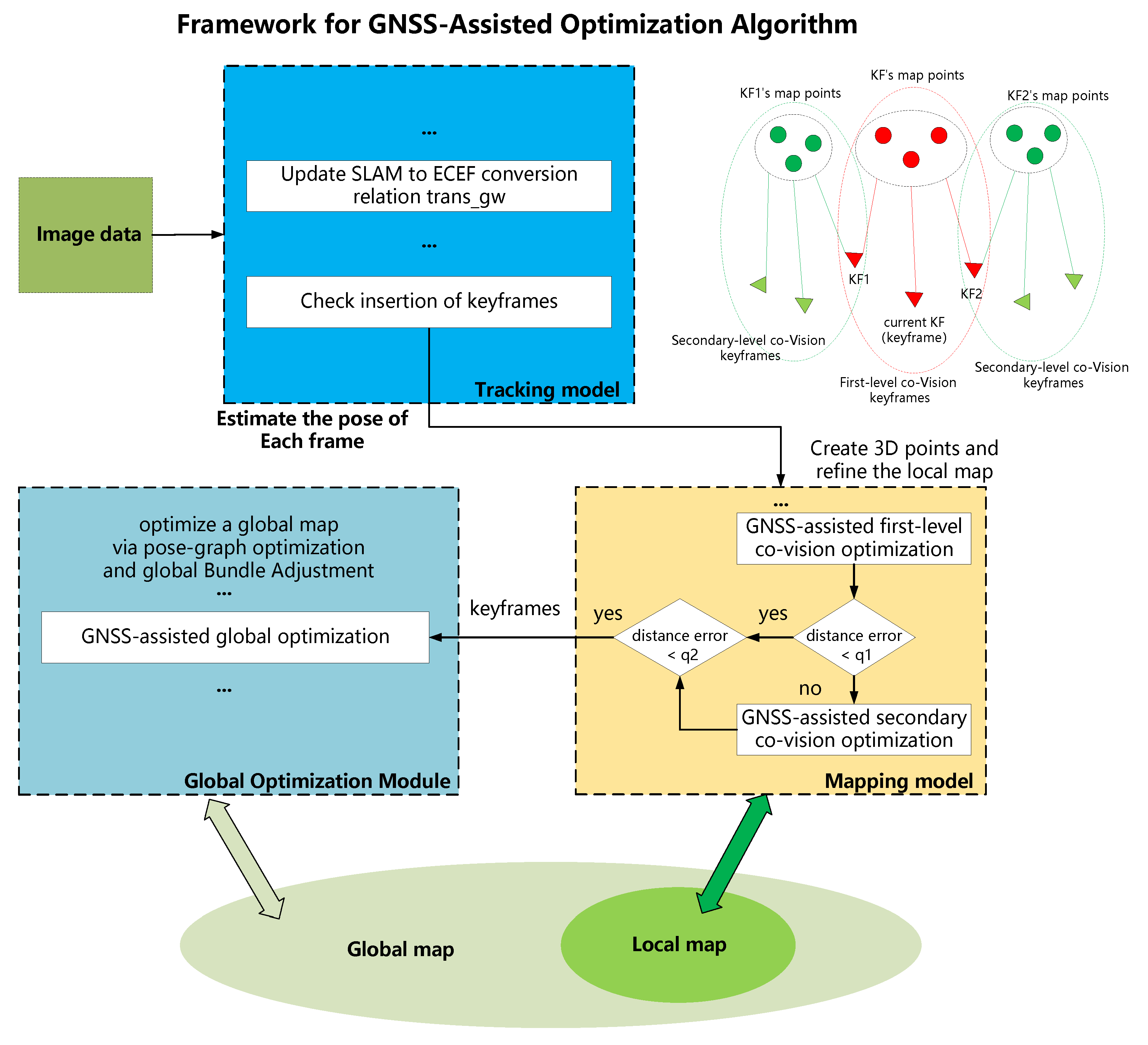
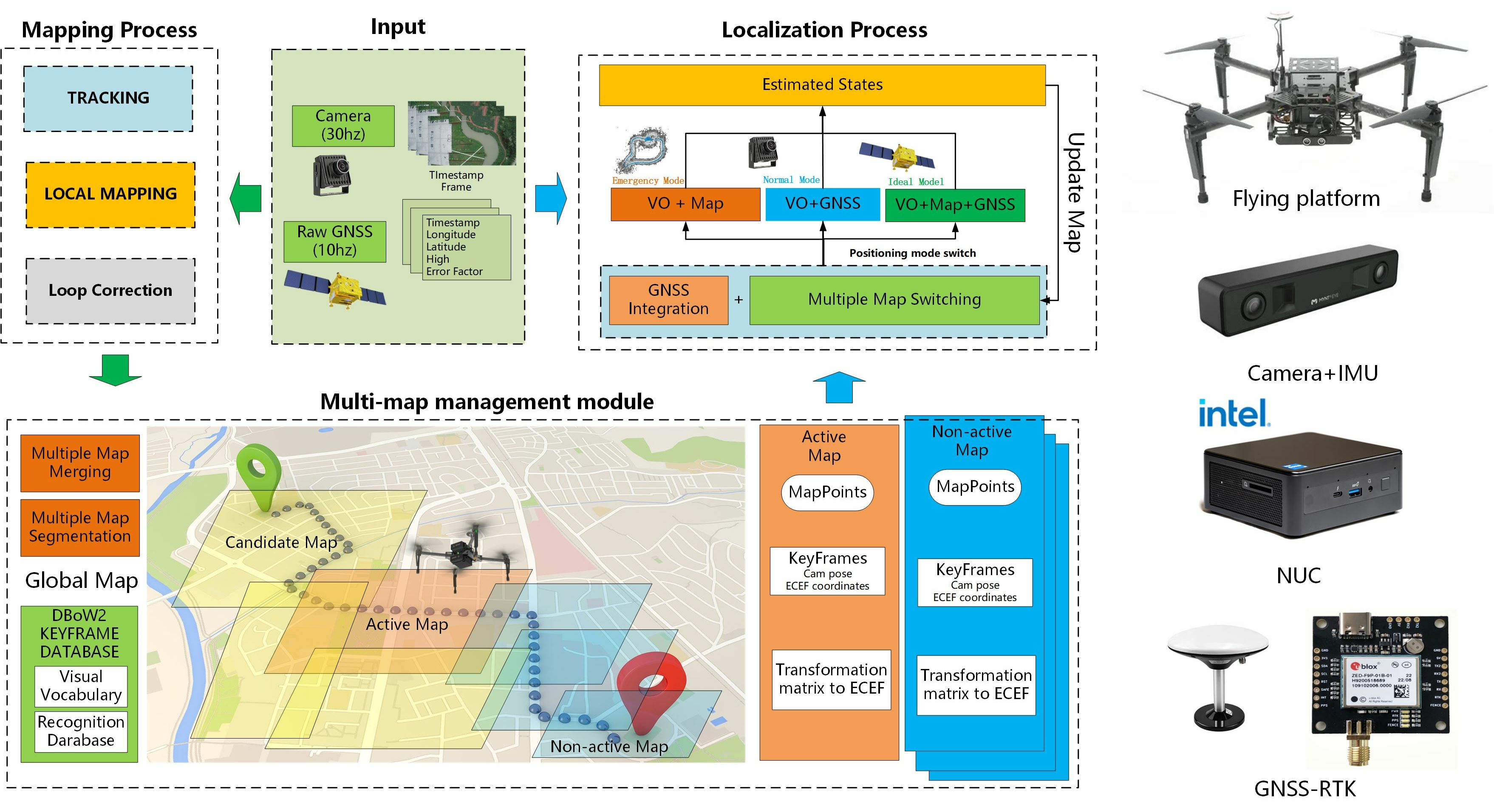
Among the various methods available, our primary focus is on integrating the complementary features of the global positioning sensor GNSS, the camera as a local positioning sensor, and high-precision multi-maps to achieve real-time and accurate state estimation in unknown environments. Combining small and low-cost sensors, such as cameras and GNSS receivers, into an integrated system makes it possible to create a robust localization system with lower construction costs, reduced complexity, and easier integration. Based on the objectives above, we developed a robust and accurate multi-map system with GNSS assistance for long-distance visual navigation. This system is designed to achieve continuous, robust, and precise localization in large-scale and complex environments. Firstly, the system utilizes low-cost visual odometry to independently provide accurate and high-frequency pose estimation in the short term, unaffected by external environmental disturbances or signal losses. The system employs place recognition techniques to match the observations with elements in previously visited areas, allowing for drift reset and utilizing pose graph optimization or bundle adjustment (BA) for map correction with higher accuracy. Secondly, the system reduces the accumulated errors of pure visual odometry by formulating a GNSS-visual multi-sensor fusion optimization algorithm on the factor graph. This approach enables accurate initialization and absolute localization in large-scale environments. The system can easily integrate measurements from other sensors as new factors into the framework. Then, with GNSS assistance, the system automatically creates multiple high-precision maps based on the scenes encountered. These maps encompass diverse geographical locations and periods. Constructing multiple maps at different times and seasons allows the system to cope with complex environmental changes, thereby maximizing the robustness of visual matching. Finally, during the online localization phase, if the GNSS signal is lost for an extended period, the system seamlessly switches to using the high-precision multi-maps as a substitute for GNSS to continue providing global positioning information for the aircraft. This approach prevents degradation to the pure visual odometry mode, which could lead to accumulated errors and localization failures. The main contributions of this paper are as follows:

• We propose a graph optimization model that combines GNSS data and visual information using multi-sensor fusion navigation and positioning technology. This model establishes optimization constraints to enhance overall positioning and mapping accuracy.
• To enhance the accuracy and robustness of large-scale map construction, we propose a method for partitioning visual maps based on the health condition of the maps. By considering factors such as feature quality, pose accuracy, and coordinate system transformation errors, the method effectively divides extensive scenes into appropriate segments to create multiple maps.
• To address the issue of excessive discrete maps leading to resource wastage and reduced map-switching efficiency, we propose a multi-map-matching and fusion algorithm based on geographical location and visual information. Unlike the standard bag-of-words model, we employ GNSS assistance to detect overlapping areas, accelerating detection speed and reducing false matches from similar scenes. By performing map fusion, the integrity of the SLAM operation area is maximized, and the system’s robustness in long-distance visual navigation is enhanced.
• This paper proposes a multi-map-based visual SLAM online localization algorithm that robustly manages and coordinates multiple geographical maps in different temporal and spatial domains. The working area of UAVs and eVTOL is divided into a grid-like structure, and the map coverage of each grid cell is recorded and stored. When the visual navigation system fails to locate a grid cell or the localization accuracy is insufficient, the system selects a new map from neighboring cells based on multi-map grid information.

Based on the aerial drone experimental platform we established, we created a test dataset for aerial drone navigation and positioning, covering long distances (on the order of tens of kilometers). The proposed system was extensively evaluated in both simulated and real-world environments. Based on our experimental results concerning the potential degradation or unavailability of GNSS positioning for UAVs and eVTOL in complex environments, we achieved an average positioning accuracy of 1.5 m over a flight distance of up to 30 km using only a monocular camera and multiple maps. The system offers advantages in construction cost, complexity reduction, and ease of integration, enabling continuous, robust, and precise localization in large-scale and complex environments. Compared to the solutions commonly used in the industry, our system offers lower costs, reduced complexity, and easier integration while ensuring the precision of localization for UAVs and eVTOL.

2. Related Work

Based on image information, the visual front-end computes the initial values of camera motion, which include indirect methods based on feature points and direct methods based on grayscale information. The back-end processing primarily involves optimizing front-end parameters on a larger scale, including tasks like filter optimization and nonlinear optimization. On the other hand, loopback detection is mainly concerned with scene identification and accomplishes closed-loop detection using local and global descriptors.

2.1. Visual SLAM

In 2003, Davison et al. proposed the first pure visual monocular SLAM system, which achieved real-time and drift-free performance using a structure motion model [16]. MonoSLAM [16] monitors relatively sparse feature points in the front end, utilizing the extended Kalman filter (EKF) and Shi–Tomasi points for solving. It employs guided search based on correlation to track the feature points in subsequent images. However, as the map size increases, the computational complexity and processing time also increase.

Keyframe-based techniques are more accurate for the exact computational cost than filtering methods and have evolved into classical standards in developing Visual SLAM and visual odometry (VO). In 2007, Klein et al. introduced PTAM (parallel tracking and mapping) as presented in [17], which achieved parallel processing for both camera tracking and map construction processes and implemented the keyframe mechanism. In contrast, keyframe-based methods use only a few selected frames to estimate the map, discarding information from intermediate frames. This approach allows for more time-consuming and more accurate bundle adjustment (BA) optimization at keyframe rates. Using sliding window BA techniques, a large-scale monocular SLAM system was implemented as described in [18]. Additionally, dual window optimization and visibility graphs were explored for implementation as detailed in [19].

Building upon these ideas, ORB-SLAM [5] achieves large-scale monocular SLAM through the utilization of sliding window BA. The ORB-SLAM system is designed around a framework with three parallel threads: front-end tracking, local map building, and back-end loop closure detection and optimization. ORB-SLAM utilizes ORB feature point detection and employs the DBoW2 library [20] for loop closure detection and relocalization purposes. By leveraging the complete set of feature points, ORB-SLAM achieves extremely high localization accuracy while maintaining real-time performance. In 2020, Fu, Qiang, and Yu published a paper on FastORB-SLAM, which presents a lightweight and efficient method. This approach tracks key points between adjacent frames without the need for computing descriptors [21].

OpenVSLAM [22] is a visual SLAM framework known for its high usability and scalability. The system incorporates monocular, stereo, and RGBD visual SLAM methods. One of the critical aspects is the ability to create maps that can be stored and loaded, allowing OpenVSLAM to localize new images using prebuilt maps. However, one limitation of OpenVSLAM is that it creates single independent maps. Once the tracking is lost, it cannot create new maps, and it lacks a module for multi-map switching and merging. Indeed, OpenVSLAM solely relies on visual information for mapping and localization without incorporating a fusion of global positioning sensor data, such as GNSS. This can lead to significant cumulative errors in long-distance localization, resulting in failures during loop detection and global optimization.

In contrast, the direct method eschews feature extraction. It directly utilizes the pixel intensity in the image to estimate motion and reconstruct a 3D map of the environment by minimizing photometric errors. In 2014, Jakob Engel et al. proposed the large-scale direct monocular SLAM (LSD-SLAM) approach [23], which enables the construction of large-scale consistent maps and the real-time reconstruction of keyframe-based pose maps and semi-dense 3D environmental maps. However, the map estimation is limited to pose graph (PG) optimization, which falls short in accuracy compared to PTAM and ORB-SLAM [5]. The hybrid system SVO (semi-direct visual odometry) [24,25] employs FAST feature extraction, utilizes the direct method to track features and inter-frames with any pixel having a non-zero intensity gradient, and optimizes camera trajectory and 3D structure through reprojection error.

SVO is highly efficient; however, as a pure visual odometry method, it only matches map elements obtained within the last few seconds, which limits its accuracy. In 2016, Engel et al. introduced DSO (direct sparse odometry) technology [7], which is a novel, high-precision, sparse direct method for visual odometry. It is based on innovative formulations for both structure and motion estimation. The proposed framework includes comprehensive photometric calibration, considering the lens’ exposure time, vignetting effects, and non-linear response function. Direct sparse odometry (DSO) can accurately compute the camera’s pose even when point detectors perform poorly, enhancing robustness in low-texture areas or blurry images. It introduces local photometric BA while simultaneously optimizing the camera poses of the seven most recent keyframes and the inverse depth of the points. Extensions of this work include stereo visual odometry [26], incorporating feature and DBoW2 [27,28] for loop closure detection, and visual-inertial odometry [29]. Direct sparse mapping (DSM) [30] introduces the concept of map reuse in direct methods, enabling zero-drift performance when the system moves through previously mapped regions. This highlights the significance of map reuse in direct visual odometry systems.

Ayham Shahoud et al. introduced the utilization of geometric information from street intersection layouts in urban environments to compute necessary data in unmanned aerial vehicle (UAV) visual navigation [31]. They addressed position drift through scene matching to mitigate cumulative errors in visual odometry and conducted testing within a simulated environment. There might be certain limitations associated with the application of these methods in our task. Unmanned aerial vehicles and vertical takeoff and landing electric aircraft are employed in our task scenario for autonomous cargo transportation and human commuting. The regions where the tasks are carried out encompass not only urban areas but also substantial suburban regions lacking city streets. Ayham Shahoud and his colleagues’ approach necessitates prior knowledge of the dimensions of street scene matching, which becomes challenging to acquire for purely natural environments. If unreasonable scale or angle values are obtained, matching with landmarks does not occur, leading to continued drift in visual odometry. Overall, leveraging street geometry edge information to enhance feature detection capabilities in urban environments offers a promising avenue for future expansion.

Considering these features, we adopt a multi-threaded framework in our system, including front-end tracking, local map construction, back-end loop closure detection and optimization, and multi-map management. The front end utilizes monocular vision, employing ORB feature point detection and using the DBoW2 library [20] for loop closure and relocalization. Based on keyframes, we perform BA optimization in the back end. During the online localization stage, we enhance the robustness of relocalization through map reuse techniques. However, these methods can only address SLAM problems in small-scale scenarios. Without global localization information fusion, UAVs may experience significant cumulative errors during long-distance flight and visual navigation. Therefore, we introduce a multi-sensor fusion optimization approach based on GNSS assistance.

2.2. Multi-Sensor Fusion SLAM

In complex outdoor environments, there is excellent research interest in integrating camera data with other sensor data for data fusion-based localization methods. This interest stems from the need to enhance the sustained stability of individual cameras.

2.2.1. Combining Images and IMU for Robust Visual

In 2007, Mourikis and his colleagues introduced the filter-based VIO algorithm [32] (multi-state constraint Kalman filter), which integrates IMU and visual data within the extended Kalman filter framework. The first tightly coupled visual odometry system based on keyframes and bundle adjustment is OKVIS [33,34]. It is capable of utilizing both monocular and stereo vision data.

ORB-SLAM-VI [35] introduced a visual-inertial SLAM system that, for the first time, enables the reutilization of the map by associating short-term, medium-term, and long-term data. By utilizing IMU preintegration [36,37], accurate local visual-inertial bundle adjustment (BA) has been achieved. However, the slow initialization of the IMU imposes limitations on the robustness and accuracy of the system. In ORB-SLAM3 [9], the system is built upon ORB-SLAM-VI and extended to include stereo visual-inertial SLAM capabilities. Camera position prediction is achieved using the inertial navigation system (INS) to assist ORB feature tracking instead of relying on unreliable temporary motion models. Christian Forster and his team addressed the real-time optimization problem of IMU by integrating inertial measurements between selected keyframes into a single relative motion constraint [37]. Indeed, their approach overlooks the noise characteristics of the IMU and minimizes the three-dimensional errors of points in space rather than their reprojection errors. Recently introduced, BASALT [38] is a stereo visual-inertial odometry system that extracts nonlinear factors from visual-inertial odometry for use in bundle adjustment (BA). By closing loops through matching ORB features, BASALT achieves excellent accuracy, ranging from very good to outstanding. Kimera [39] is a novel and outstanding metric semantic mapping system. Its measured component includes stereo inertial odometry and utilizes DBoW2 and pose graph optimization for loop closure, achieving accuracy similar to VINS-Fusion.

In 2018, the Hong Kong University of Science and Technology introduced VINS Mono [8], which is a monocular visual-inertial odometry system with loop closure detection. It has the capability of loop closure detection, which utilizes DBoW2 and 4-degree-of-freedom pose graph optimization. VINS-Mono is a relative positioning method that provides state estimation in the local coordinate system. VINS-Mono [8] utilizes a sliding window optimizer for pose estimation; however, their estimator predominantly relies on frequent visual observations. The front end of VINS-Mono adopts keypoint extraction followed by optical flow-based tracking. Consequently, it exhibits limited robustness and accuracy in environments with weak textures and a scarcity of key points. The absence of feature descriptor extraction and the reliance solely on optical flow-based tracking makes the system susceptible to camera loss or blurriness in the visual input, and it lacks a relocalization module. As a result, motion on nearly planar road surfaces can render the scale estimation in VINS-Mono unobservable. In constant velocity motion, the IMU has one unobservable degree of freedom, leading to drift. Despite VINS-Mono’s [8] ability to observe roll and pitch angles using monocular visual-inertial navigation, for unmanned aerial vehicles, using ORB features as utilized in ORB SLAM [5] would be more advantageous for rotation-invariant features.

In 2019, a novel initialization approach was proposed in VINS-Fusion [11]. The VINS-Mono system has since been extended to include stereo vision and inertial capabilities. To achieve multi-position fusion, the extended VINS-Mono framework combines KF-INS, GNSS [40], and VINS-Mono. The PL-VINS algorithm developed by Fu et al. [41] integrates line features into VINS and optimizes the frontend system. In 2022, Nianzu Gu et al. utilized VINS-Fusion to analyze the VIG system’s performance under GNSS spoofing attacks [42]. They proposed a global pose graph matching method for areas with multiple revisits in integrated systems.

Ultimate SLAM maximizes the complementary advantages of event and conventional cameras, enhancing the robustness and stability of visual SLAM in extreme scenarios [43]. Event cameras are not affected by motion blur and possess an exceptionally high dynamic range, enabling them to provide reliable visual information in scenarios involving high-speed motion or high dynamic range features. Event cameras, functioning as local positioning sensors, cannot provide global positioning information, thus making them incapable of mitigating the cumulative error issues in long-distance navigation.

2.2.2. Combining GNSS, Images, and IMU for Robust Visual

By employing real-time kinematic (RTK) technology [44], GNSS can achieve centimeter-level positioning in open-sky environments. In VINS-Fusion [11], GNSS is integrated into the global estimator based on the VINS-Mono [8] system, where the local estimator is a VINS. GNSS can aid in estimating IMU biases, but in [11], the GNSS and VINS estimators are decoupled. In GVINS [12], GNSS raw measurements are tightly integrated into VINS, enabling global localization in both indoor and outdoor environments. The method proposed in GVINS [12] is based on VINS-Mono [8] but no improvements were made to the visual processing. Therefore, GVINS may experience reduced robustness and accuracy in environments where GNSS is unavailable.

In [45], GNSS/INS integration and VINS are simultaneously activated to initialize a GNSS-visual-inertial navigation system for a land vehicle. However, this approach is weakly coupled. G-VIDO [14] is a similar system, but it further incorporates vehicle dynamics to enhance the accuracy of the system. G-VIDO [14] proposes a vehicle dynamics and intermittent GNSS-aided visual-inertial odometry state estimator to address the localization problem of autonomous vehicles, specifically, the estimation of position and orientation in a global coordinate system under various GNSS conditions. The algorithm is primarily designed to address the localization problem of autonomous vehicles, specifically estimating the position and orientation in a global coordinate system under various GNSS conditions. G-VIDO [14] robustly initializes the proposed highly nonlinear system by loosely aligning the results of monocular structure from motion (SfM), pre-integrated inertial measurement unit (IMU) measurements, and vehicle motion information. Firstly, G-VIDO [14] has limited usage scenarios. Based on the two-degree-of-freedom vehicle dynamics model, G-VIDO proposes the theory of dynamic pre-integration and constructs dynamic constraints in the optimized backend to consider the issue of unobservable problems in monocular visual-inertial systems under degenerate motion. While this model improves the positioning accuracy of ground vehicles, it cannot be directly applied to the positioning problem of aerial drones. Our system is not limited by usage restrictions on aerial or ground robots; it serves as a universal framework for integrating monocular visual sensors with GNSS positioning and multi-map construction. Secondly, the front-end of G-VIDO [14] utilizes the Harris corner detection algorithm to detect new feature points and employs the KLT algorithm for sparse optical flow tracking. Our system utilizes ORB feature point matching for front-end tracking, which offers better rotational invariance and is more advantageous for the flexible aerial tracking and positioning of drones. Lastly, G-VIDO [14] cannot perform long-distance navigation under prolonged GNSS signal loss conditions. Both our algorithm and G-VIDO adopt monocular visual-inertial GNSS integration for positioning. Both use GNSS for reference coordinate system conversion and constraint construction in the sliding window and for employing sliding window and loop closure detection strategies for optimization. With the assistance of GNSS, accumulated errors can be corrected, and the vehicle’s position in the global coordinate system can be determined. GNSS anomaly detection algorithms are employed to enhance the robustness of the system under intermittent GNSS conditions. In contrast, G-VIDO [14] incorporates intermittent GNSS measurements to mitigate cumulative errors. Additionally, G-VIDO solely functions as a state estimator and does not include constructing a multi-map system. In the event of sudden GNSS signal interruption, positioning error may be temporarily increased. In the event of complete long-term GNSS signal loss, it inevitably results in a significant increase in cumulative error during long-distance navigation. Although G-VIDO [14] has conducted experiments in a GNSS-deprived environment and compared it with VINS-FUSION, they only tested the system over a ground distance of just over 800 m, which is insufficient to demonstrate its superior positioning accuracy over long distances (several tens of kilometers). Our system can construct high-precision visual maps in the offline phase, providing global positioning information as a substitute for GNSS.

In [46], tightly coupled, optimization-based GNSS-visual-inertial odometry is proposed; however, GNSS does not contribute to the initialization of the visual system. GNSS can assist in completing the initialization of INS and, subsequently, VINS. As a result, GNSS and VINS can operate in a unified global coordinate system without additional conversions. IC-GVINS [13] proposes a robust real-time inertial navigation system (INS)-centered GNSS-visual-inertial navigation system (IC-GVINS) for wheeled robots. Both VINS-Mono [8] and IC-VINS [13] are sliding-window visual inertial navigation systems (VINSs). Compared to VINS-Mono, IC-VINS has made improvements in various aspects of its front-end, such as feature detection, feature tracking, and triangulation, as well as in its back-end, including IMU preintegration and outlier handling. The INS-centered design encompasses several components, including a precise INS with Earth rotation compensation, GNSS-assisted initialization, and INS-assisted visual processing. IC-GVINS [13] performs well in indoor environments; however, in outdoor settings, it may be affected by weather and environmental conditions, which can lead to drift issues.

The analysis of the three modules above demonstrates that the multi-sensor fusion-based localization method significantly enhances the robot’s positioning accuracy. The camera and IMU work in local coordinate systems for outdoor large-scale navigation and localization, so it is ideal for fusing GNSS global information to reduce cumulative errors. Existing GNSS-assisted methods can work during intermittent GNSS signal losses. However, in cases of complete GNSS signal loss, they degrade to a purely local sensor positioning mode, inevitably leading to cumulative errors. Furthermore, these approaches predominantly emphasize real-time state estimation, with less emphasis on multi-map construction. UAVs and eVTOL must have alternative solutions to continue providing global positioning information in the event of GNSS signal loss. Considering that the cameras and IMU (inertial measurement unit) operate in local coordinate systems, there are several issues to address in UAV flight, such as significant disturbances on the IMU caused by high-frequency vibrations. Moreover, extensive research has been conducted on integrating cameras and IMU for navigation. Existing GNSS-assisted methods can work during intermittent GNSS signal losses. However, in cases of complete GNSS signal loss, they degrade to a purely local sensor positioning mode, inevitably leading to cumulative errors. Among the numerous methods available, our primary focus lies in effectively integrating the complementary features of the global positioning sensor GNSS, the local positioning sensor from the camera, and the high-precision multi-map data. We aim to explore how these components can be combined to enhance navigation accuracy. Furthermore, our approach is designed to be extendable to incorporate other methods in the future. Hence, our system proposes a health-based SLAM multi-map construction method. Under normal circumstances, we utilize GNSS assistance to optimize and establish high-precision maps. When GNSS signals are disrupted or lost in emergency scenarios, our proposed multi-map-based visual SLAM online localization method comes into play. This method allows us to select suitable maps to continuously provide global positioning information for UAVs and eVTOL, providing an additional assurance layer.

2.3. Multi-Map SLAM

With the advancement of SLAM technology, the advantages of multi-map SLAM lie in enhancing the robustness of localization by utilizing map construction and fusion to mitigate tracking loss during the positioning process [35]. Enhancing robustness against tracking loss through map creation and fusion during exploration was first proposed in the filtering-based approach presented in [47]. One of the earliest keyframe-based multi-map systems was introduced in [48]. However, the map initialization in this system was manual, and it could not merge or associate different sub-maps. Multi-mapping capability has been studied as a component of collaborative mapping systems, which include multiple mapping agents and a central server that only receives information [49]. Alternatively, there are systems with bidirectional information flow, such as C2TAM [50]. MOARSLAM [51] proposes a robust stateless, client–server architecture for collaborative multi-device SLAM. However, it primarily focuses on the software architecture and does not report accurate results.

Recently, CCM-SLAM [52,53] introduced a distributed multi-drone multi-map system based on ORB-SLAM featuring bidirectional information flow. Their focus was on overcoming the challenges of limited bandwidth and distributed processing. SLAMM [54] also proposed a multi-map extension system based on ORB-SLAM, further enhancing accuracy.

ORB-SLAM3 [9] is a multi-map SLAM system capable of handling monocular, stereo, and inertial visual systems. They improved the localization approach to enhance accuracy in loop closure scenarios. Additionally, they employ local bundle adjustment (BA) to achieve more detailed and accurate map fusion. Based on ORB-SLAM3 [9], the system can survive for extended periods when visual information is incomplete. When it experiences a loss of tracking, it initiates a new map and seamlessly merges it with the previously constructed map upon re-encountering it. This ability allows it to maintain localization and mapping performance even in challenging visual conditions.

Liu et al. improved the reliability of ORB-SLAM3 [9] in real-time dynamic environments by introducing semantic threads and semantic-based optimization threads. The author enhanced map fusion and search efficiency by leveraging semantic information [55]. Dengming et al. proposed a local multi-map fusion method for pure visual map fusion in extreme environments. The method addresses the problem of selecting rapid relocalization or constructing a new local map from the current position when tracking is lost [56]. Traditional multi-map matching and fusion utilize DBoW (DeBoW) bag-of-words; however, setting a fixed similarity threshold for DBoW2 can be challenging. To overcome this matching issue, Liu Boyang et al. integrated the KNN map-matching method into a collaborative visual-inertial SLAM system [57].

Ceyhun Karpuz et al. introduced a collective robot localization algorithm inspired by model-matching-based positioning systems [58]. Specific data collection and localization calculations are performed during the offline phase, while a specific data exchange is carried out during the online phase. Employing multi-robot collaboration to accelerate data collection and mapping speed would be a valuable application.

Based on the multi-map characteristics, our system introduces a multi-map management module. However, most traditional multi-map systems built based on purely visual or local localization sensors like IMUs tend to accumulate errors, making them unsuitable for long-distance mapping applications. Additionally, since these maps lack relative positional information, they cannot be fused without overlapping areas, leading to disconnected states in the mapping process. Our system enhances map accuracy in long-distance mapping by introducing GNSS-assisted optimization during the mapping process. The algorithm can generate new maps when tracking fails by establishing multiple maps, ensuring continuous mapping and information preservation. Later, the maps are merged during loop closure, allowing for seamless integration. GNSS global positioning information can merge these maps into a single global coordinate system, even if they lack overlapping areas. Compared to traditional algorithms that rely on visual loop closure to detect overlapping areas between two maps, especially in exceptional cases where visual relocalization fails and results in overlapping area detection failure, our system can utilize GNSS information to detect map overlapping areas, further improving the speed and effectiveness of the detection process. Under unstable or missing GNSS signals, the reuse of multiple maps allows for continued global positioning information for UAVs and eVTOL.

3. System Overview

The proposed system employs a feature-based visual SLAM algorithm and incorporates GNSS data as an offline tool to create a comprehensive multi-map. The system can operate in either purely visual or visual GNSS mode, enabled by using a monocular camera capable of both pinhole and fisheye configurations. The overall framework of the system is shown in Figure 1.

3.1. System Module

(1) Multi-map management module: This module manages a set of discrete maps divided into two groups: the current active maps and the non-active maps. While inserting more keyframes into the map and constructing additional map points, the tracking thread continues to use the active map for image frame localization. When the active map is insufficient to meet the current localization requirements, the system employs a strategy based on the current position to select candidate maps from the non-active maps. The system can dynamically switch within these candidate maps to find the map that provides the highest relocalization accuracy.

(2) Tracking thread: This system performs the real-time processing of sensor data and calculates the current frame pose relative to the active map to decrease reprojection errors of matching map features. Additionally, it determines whether the current frame should be a keyframe. If the system is in localization mode and tracking is lost, the multi-map management module sorts the candidate map queue using GNSS data and repeatedly switches until the reset is successful. In mapping mode, the system saves the active map before creating a new map.

(3) Local mapping thread: This system optimizes the active map by incorporating newly acquired keyframes and map points while removing excess ones. It utilizes visual and GNSS data to minimize reprojection errors and GNSS range errors as residual terms. Furthermore, based on the GNSS range error threshold of the current frame, a multi-level optimization strategy is implemented by leveraging co-visual keyframes at multiple levels. The term “co-visual keyframes” refers to keyframes that observe common map points.

(4) Global optimization thread: This system continuously checks for overlapping areas between the current keyframe and the active map, performing a loop correction if required. The algorithm also monitors the GNSS range error of the current frame and initiates global optimization if it exceeds a set threshold by adopting the complete map for optimization.

3.2. System Working Mode

We illustrate the working model through a specific application scenario. Suppose we have an aircraft intended to frequently perform cargo or passenger transport missions within a specific area. In most cases, GNSS signals are normal. Occasionally, there may be temporary signal loss due to poor signal quality. A worse scenario is when someone intentionally interferes with the signals, resulting in prolonged GNSS signal loss. In long-distance navigation tasks, the absence of auxiliary optimization using GNSS global information can result in significant positioning errors due to accumulated errors. The system primarily operates in two main modes: mapping mode and positioning mode.

3.2.1. Mapping Mode

During the online map-building stage, when most GNSS signals are reliable, the initial step involves employing an aircraft to traverse the designated mission area. Simultaneously, the area’s image information and GNSS data are recorded, enabling their utilization for subsequent map construction and optimization. The high-precision map that has been established integrates GNSS data and is used for subsequent tasks involving global navigation and positioning.

In our primary application scenario, the aircraft performs multiple logistics and manned transportation missions within a designated area spanning several tens of kilometers. In most cases, the aircraft follows the planned flight path to execute the mission within the predefined map area. However, there may be exceptional circumstances, where the aircraft may fly outside the predetermined map area. We primarily address the degradation issue through two main approaches.

On the one hand, we aim to reduce purely linear trajectories by setting the flight path. Firstly, in the design of the flight path, we strive to avoid long straight-line trajectories as much as possible. For instance, in our experiments, we utilize curved flight paths. Secondly, if there are long linear flight paths, we set the flight altitude to vary within a certain range instead of maintaining a constant height. For example, we may set the altitude to vary within 10–20 m. Lastly, in the mapping stage, we employ multiple overlapping strips near the same flight path to ensure that adjacent strips can recover information from any missed strips.

On the other hand, our system typically performs online real-time map construction to obtain positioning results more quickly. The computation and optimization of the similarity transformation from the vSLAM coordinate system to the geodetic coordinate system for newly created maps are performed within a separate global optimization node following the loss of tracking. This process does not impact the real-time local mapping procedure. Successful computation can still be achieved when incorporating the positioning data of nonlinear trajectory points. In extreme cases, the system cannot obtain positioning data from the nonlinear trajectory phase. However, during the mission execution, both GNSS information and image data are consistently saved. Due to multiple flight strips covering the same flight path, this information is recovered and resolved through offline mapping once all the data collection is complete. Offline mapping utilizes global information, and the obtained images and poses can be manually controlled, resulting in higher accuracy levels.

3.2.2. Positioning Mode

During the offline positioning stage, the aircraft re-enters the designated area to execute the flight mission, although there may be instances of deviation from the mission area. In this mode, various scenarios need to be taken into consideration. Figure 1 depicts the functional working model, specifically in the “Positioning Processes” section.

The ideal model incorporates a combined positioning mode that integrates VO, GNSS, and GNSS Map. In the ideal scenario, the GNSS signals are stable and reliable for an extended period, and a valid and reliable high-precision visual map is established. Real-time pose estimation is achieved by combining the global GNSS positioning information, local VO positioning, and the established map, enabling continuous updates of the map elements. In this mode, even if the unmanned aerial vehicle (UAV) flies outside the mission area, the map continues to update and expand. We can consider this mode as returning to the online mapping stage.

The normal mode employs a combined positioning mode that integrates VO and GNSS. Despite pre-building the visual map, there may be extreme cases where relocalization could be unsuccessful. For example, significant changes in the landscape can occur due to seasonal transitions. However, in this mode, with the availability of strong GNSS signals, it is possible to utilize both local VO and global GNSS to reconstruct a new map and achieve real-time positioning dynamically. The newly established map is merged with the multi-map system to expand the utilization scenarios of the maps. We can consider this mode as reverting to the online mapping stage. However, this mode occurs relatively infrequently because the aircraft performs frequent missions within the same area, resulting in continuous map updates.

The emergency mode utilizes a combined positioning mode that integrates VO and a GNSS Map. This is the most commonly used operational state. Under normal circumstances, during mission execution, there may be brief periods of GNSS signal loss and even prolonged complete loss due to malicious interference. In such situations, the global map is utilized to continue providing global positioning information and to enable real-time updates of the map elements. In this mode, if the unmanned aerial vehicle (UAV) flies outside the mission area, although the map continues to update and expand, there is a certain range beyond which the map updates cease. Due to the absence of GNSS signals, expanding the map using purely visual information outside the mapped area is considered unreliable.

During actual flight missions, the system automatically switches between multiple modes based on the prevailing conditions to adapt to most situations. The continuous real-time updating and saving of the map in the first three modes prove advantageous in supplying the most recent map data to other aircraft. These high-precision maps effectively address the issue of accumulated errors in pure visual localization mode and serve as a substitute for GNSS in providing global positioning information.

4. GNSS-Visual-Multi-Map Navigation System Based on Graph Optimization

In long-distance visual navigation, relying solely on pure vision as a local positioning sensor cannot avoid mapping errors caused by scale drift. As the navigation time increases, reliance on loop closure correction becomes necessary to suppress accumulated errors. However, forming loop closure conditions in large-scale environments becomes challenging, leading to unavoidable error accumulation. However, as a standard sensor data, GNSS has minimal cumulative errors and provides relatively accurate global positioning information. It can effectively compensate for the visual deficiencies mentioned above. We propose a GNSS-vision fusion mapping algorithm based on dynamic range graph optimization. It utilizes multi-level thresholds to control distinct optimization ranges, enhancing and improving visual SLAM mapping accuracy. By leveraging the complementary characteristics of visual and GNSS information, we design a graph optimization model that combines the least squares method to construct optimization constraints. This approach effectively addresses the limitations and vulnerabilities of a single navigation system.

The algorithm framework for the optimization module is shown in Figure 2. The optimization process includes both the global and local optimization of the map. Since mapping and optimization are carried out on separate threads, the global optimization module can only commence processing the current keyframe after the mapping module has completed its requisite processing. Nevertheless, not all inserted keyframes undergo optimization. To effectively control the optimization area, when the number of vertices and edges in the graph optimization model is large, the optimization process may become resource intensive, potentially impacting the system’s normal operation. Therefore, the optimization algorithm designed in this study dynamically controls the scope of the map optimization based on the current frame’s GNSS distance error. Relying solely on pure vision as a local positioning sensor cannot avoid mapping errors caused by scale drift.

In the tracking module, after estimating the pose of each frame of the image, the system calculates the transformation relationship, denoted as $tran{s}_{gw}$, between the current SLAM and the ECEF (earth-centered, earth-fixed) coordinate system based on all existing keyframes in the map. After generating a new keyframe and completing the local map update, the mapping module optimizes the first-order co-visibility relationship assisted by GNSS. Subsequently, the GNSS distance error for the current keyframe is computed. If this distance error exceeds the threshold q1 set by the system, the GNSS-assisted secondary visual co-visibility optimization operation is initiated to expand the scope of optimization. With that, the optimization process of the mapping module concludes. After completing the mapping module, the current keyframe is passed on to the global optimization module. In this module, the GNSS distance error for that keyframe is reevaluated, and if the error exceeds the threshold q2, the GNSS-assisted global optimization process is initiated.

The threshold q in the optimization process is mainly determined based on the size of the mapping scene and the estimated distance error. For example, autonomous driving road data often have a significant variation in perspective and substantial influences from lighting conditions and dynamic changes. Consequently, errors are more likely to be more significant. However, the environmental impact is relatively minor for unmanned aerial vehicle (UAV) visual navigation data, resulting in generally smaller errors.

4.1. Local Optimization

The local GNSS-assisted optimization involves optimizing the content within the current keyframe’s first- and second-level co-visibility ranges. For the current keyframe, we refer to keyframes with at least 15 common visible map points as its primary co-visibility keyframes. Other keyframes that share the same primary co-visibility relationship with the current keyframe are called secondary co-visibility keyframes of the current keyframe. Therefore, for GNSS-assisted primary co-visibility optimization, the variables to be optimized are the pose of the current keyframe, the poses of the primary co-visibility keyframes of the current keyframe, and the set of map points observable by the keyframes above. Indeed, in addition to the mentioned keyframes, other keyframes in the map set that can observe the above set of map points also contribute to the cost function. Therefore, these keyframes also participate in the optimization computation, but their poses are kept fixed throughout the optimization process.

In the mapping thread, we use the sliding window method to optimize the posture and map point (local non-linear bundle adjustment) of the consensus key frame of the current frame. The least squares are calculated by graph optimization and realized by the Levenberg–Marquardt method in G2O [59]. On the basis of non-linear bundle adjustment (BA) in ORB-SLAM2, the key frame real GNSS and calculated GNSS residuals are added as the edge of graph optimization. Specifically, since GNSS is not a rectangular coordinate system, it is necessary to convert the LLA coordinate system, where GNSS is located to the ECEF coordinate system.

After that, the rotation matrix R and translation matrix T between the ECEF positions and the corresponding SLAM coordinate systems of all current key frames are calculated by the Umeyama algorithm. Use this dynamically maintained $tran{s}_{gw}$ matrix to convert the true values $g_{tecef}$ and system predictive value $g_{cecef}$ of the keyframes in the window to the corresponding $g_{ts}$ and $g_{cs}$ in the SLAM coordinate system. The formula for calculating the GNSS residual error is as follows:

$$E_{GNSS}\left(k\right)={{\left|\right|g_{ts}^k-g_{cs}^k\left|\right|}_{\sum }}^2$$

(1)

The original BA re-projection error refers to the result obtained by projecting the position and pose of the previous camera frame through the road mark in the map point to the camera coordinate system and then projecting it to the pixel coordinate through the internal parameter and then comparing it with the pixel position extracted from the feature. The re-projection error formula is as follows:

$$E_{vis}(k,j)={{\left|\right|x^k-\pi (R_k{X}^j+t_k)\left|\right|}_{\sum }}^2$$

(2)

where x represents the pixel coordinates of the road mark, X corresponds to the extracted detection, and $\pi$ represents the projection model.

The final optimization form obtained from the two residuals is as follows:

$$\{X^i,R_i,t_i|i\in P_L,l\in K_L\}=\underset{X^i,R_i,t_i}{argmin}\sum _{k\in K_L}\sum _{j\in X_k}{\rho }_1\left(k_1{E}_{vis}(k,j)\right)+\sum _{k\in K_L}{\rho }_2\left(k_2{E}_{GNSS}\left(k\right)\right)$$

(3)

where $K_L$ is the set of camera frames in the sliding window, $P_L$ is the set of map points visible to all camera frames in the window, and $\rho$ is a robust kernel function. Through the Huber cost function, we can eliminate the influence of edges with large errors through the threshold during the optimization process, ensuring a more robust optimization result.

We found that when the sliding window range is the first level of the common view keyframe, the local optimization map has problems because of the difference between the optimized posture and the fixed keyframe outside the window, resulting in the difficulty of subsequent optimization and increased time consumption. Therefore, the error between the current frame and the real GNSS is calculated during real-time optimization. When the error is greater than the set threshold, the sliding window range is expanded for non-linear bundle adjustment (BA).

4.2. Global Non-Linear Bundle Adjustment

Global optimization and local optimization share similar procedures. Nevertheless, global optimization expands its scope to encompass all the keyframes in the map and utilizes all the map points as well. Furthermore, due to the large number of variables to be optimized in global optimization, the system allocates additional threads to perform the optimization tasks.

Based on the original optimization, GNSS residuals of all keyframes are added as new edges by using map optimization. The calculation of residuals is similar to GNSS local BA. Because global optimization is very time-consuming, ORB-SLAM2 only performs when loopback detection is successful, and the key frame that is not updated is propagated and corrected when the keyframe is updated.

Here, we have two strategies. The process of drawing is offline construction, and the real-time requirement is not high. In order to obtain a map with better accuracy, when the error of the previous frame is greater than a set threshold (the threshold is greater than the local optimization threshold), GNSS global optimization is enabled. At this time, the mapping and tracking threads pause and wait for the optimization to end. The positioning process requires high real-time performance. Generally, we optimize the sim3 pose of the keyframe.

During the positioning process, the newly inserted keyframe participates in the optimization with the map keyframe. If the matching accuracy of the positioning image is poor, the accuracy of the original map deteriorates. Therefore, the original map fixed key frame and 3D point are fixed during the optimization process, and the results with large errors are eliminated when the key frame and map point are updated after the optimization.

GNSS-assisted global optimization is highly necessary. If only local optimization is employed, there is a possibility of “trajectory fragmentation” occurring. This is because the transformation relationship $tran{s}_{gw}$ from SLAM to ECEF coordinates is continuously updated. Due to the increasing amount of data and the presence of various errors, this value constantly changes. Indeed, due to the significant variations in the transformation $tran{s}_{gw}$, the locally optimized maps at different time instances may not guarantee global consistency.

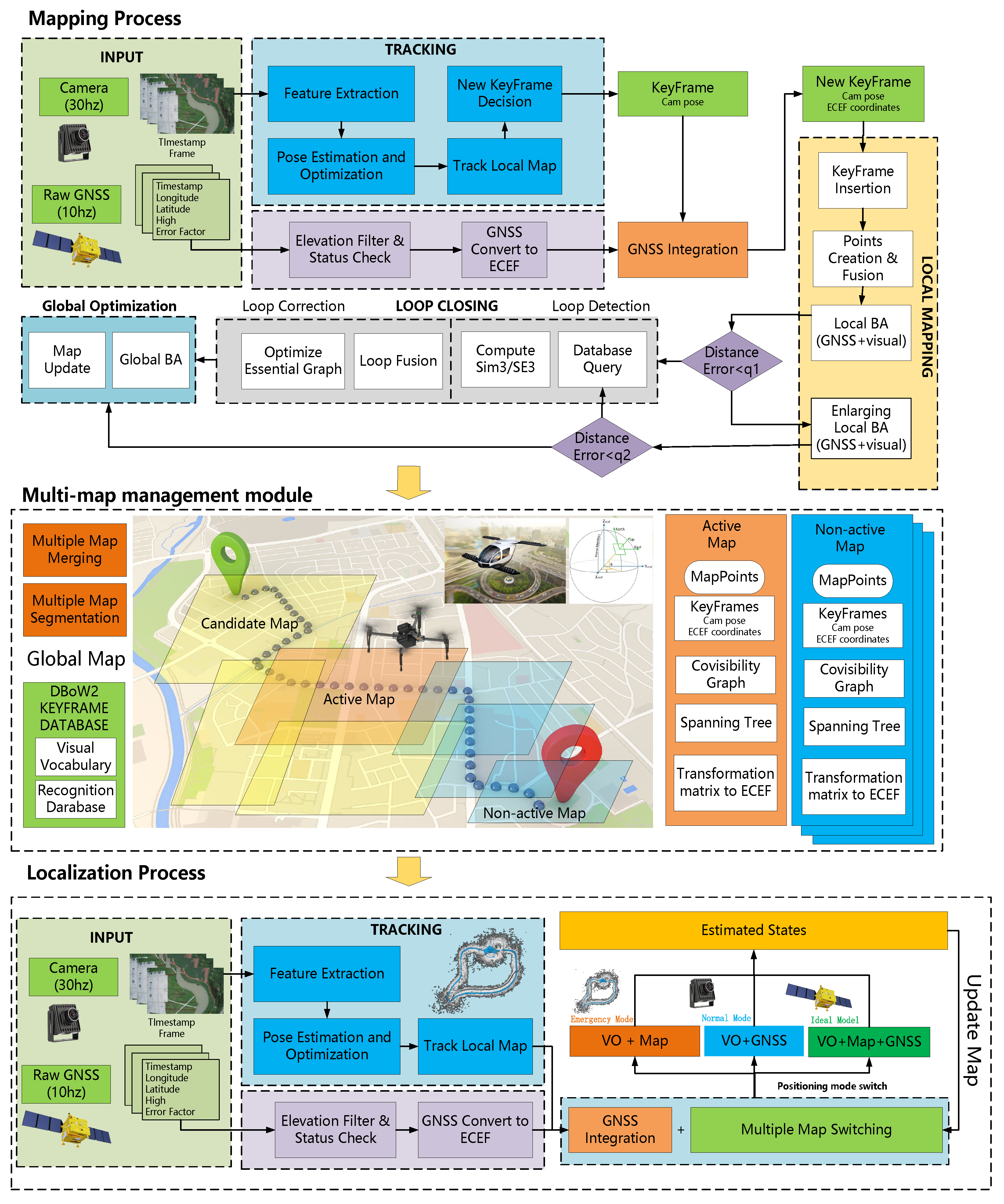
5. Multi-Map Management System

During visual navigation in large-scale environments, there are challenges posed by data redundancy resulting from long distances and dynamic variations within complex scenes. These challenges make it difficult to rely solely on a single map to fulfill the navigation tasks and requirements during the SLAM mapping and localization process. During the mapping stage, it is essential to effectively partition the large-scale environment into multiple maps based on feature quality and pose accuracy. Furthermore, in cases with overlapping areas between multiple maps, precise map fusion can be achieved automatically by integrating geographical location and visual information. The SLAM system can dynamically switch between multiple maps built offline, enabling robust and effective visual localization.

5.1. Multi-Map Auto-Segmentation

Drones and eVTOL need to divide the map for drawing when mapping large scenes. On the one hand, scale drift may occur during the map construction process in large-scale scenes due to complex terrain and image-matching errors. On the other hand, multiple maps are advantageous for loading and usage due to limited onboard resources of the equipment and issues related to map maintenance and updates. In order to improve the accuracy and robustness of large-scale map construction, this paper proposes a method of dividing SLAM maps based on their health. The health of a map reflects the quality of the current mapping process. During the tracking of each frame, the health of the current frame is calculated, and if the health value is 0, it is considered a lost frame. If more than three consecutive frames are lost during the mapping process, the currently active map is saved, and a new map construction is initiated. Health primarily comprises three aspects: the number of tracked map points, the number of inliers in the pose estimation, and the GNSS distance error.

(1) The number of tracked map points: During the tracking process of the current frame, the initial step involves constructing a frame object and extracting the feature points from it. Usually, feature points in the sky region are typically excluded to prevent significant errors caused by these points. Subsequently, different tracking modes are employed to perform image matching between the current frame and the reference frame. This process enables the establishment of a correspondence between the two-dimensional feature points in the image and the three-dimensional points in the current map. Based on these matching results, the pose estimation is carried out. Therefore, if a limited number of matching relationships is obtained, the pose estimation of the current frame becomes infeasible, and its health is considered to be 0. In practical scenarios, this reflects the significant changes that may occur between the scene captured by the current frame and the previously constructed map. These changes can include variations in texture, lighting conditions, dynamic elements, and more. In general, for UAVs and eVTOL performing repetitive tasks in the same area, these regions can be avoided through post-flight route evaluation and planning.

(2) Number of inliers in pose estimation: After obtaining the aforementioned 2D-3D matching relationships, the system performs robust camera pose estimation using PnP (perspective-n-point) and RANSAC (random sample consensus). Subsequently, nonlinear bundle adjustment (BA) optimization is conducted to refine and obtain more accurate results. If the observed points have poor geometric conditions, then the estimated pose is highly inaccurate, introducing significant errors to the subsequent mapping process. Therefore, based on the chi-square test, a threshold is calculated to determine the optimization error. This threshold is used to filter the number of inliers and outliers in the pose estimation. The reprojection error, denoted as e, is defined as the difference between the 2D position obtained by projecting using the pose and the actual detected 2D coordinates of the feature. The reprojection error follows a Gaussian distribution as shown in Equation (4):

$$e\sim N(0,\Sigma )$$

(4)

whereas the covariance matrix $\mathsf{\Sigma }$ is typically determined based on the number of pyramid levels used for feature point extraction.

If the scaling factor between pyramid layers is q and the standard deviation at the lowest layer is m pixels, the covariance calculation for the reprojection error of the detected 2D features in the current kth layer can be expressed as Equation (5):

$$\mathsf{\Sigma }={(q^k\times m)}^2\left[\begin{array}{cc}1& 0\\ 0& 1\end{array}\right]$$

(5)

Since the error e is a 2D vector, it is not straightforward to set a threshold directly. Therefore, the error is weighted by the covariance, and the inner product r of the error is computed based on Equation (6):

$$r=e^T{\mathsf{\Sigma }}^{-1}e$$

(6)

However, Equation (7) can be transformed into Equation (8), where the content within the parentheses represents a multidimensional normal distribution as shown in Equation (8):

$$r={\left({\mathsf{\Sigma }}^{-\frac{1}{2}}e\right)}^T\left({\mathsf{\Sigma }}^{-\frac{1}{2}}e\right)$$

(7)

$$\left({\mathsf{\Sigma }}^{-\frac{1}{2}}e\right)\sim N(0,I)$$

(8)

Therefore, a chi-square test threshold is designed around r. Since the projection error has 2 degrees of freedom at a significance level of 0.05, the threshold value for the chi-square statistic is 5.99. Based on this threshold, the 3D-2D relationships involved in the optimization can be filtered to identify which ones are outliers and which ones are inliers. When the number of inliers does not meet the specified threshold, the health of the current frame is considered to be 0.

(3) The GNSS distance error: This study addresses the issue of scale drift in the map construction process by introducing GNSS assistance to calculate real-time errors in the map. The current map is saved, and map construction restarts when the error exceeds the threshold range. In order to calculate the errors in the map creation process, a keyframe is included in the process to create a local map. This process uses the keyframe and its corresponding GNSS information to convert the coordinates of the model being constructed to the ECEF coordinate system, which is then used to calculate the errors. The ECEF coordinates corresponding to the current model coordinates are then determined, and the errors between these coordinates and the true values are calculated. These errors serve as the basis for map segmentation.

Assume that the model coordinates corresponding to the keyframe set are marked as ${\mathrm{P}}_{\mathrm{i}}(\mathrm{x},\mathrm{y},\mathrm{z})$. Using the iterative closest point (ICP) algorithm, the model coordinate is transformed into the ECEF coordinate system, represented by the transformation matrix in ${\mathrm{P}}_{\mathrm{i}}^{\prime }({\mathrm{x}}^{\prime },{\mathrm{y}}^{\prime },{\mathrm{z}}^{\prime })$. The conversion relationship between the two coordinate systems is shown in Equation (9).

$${\mathrm{P}}_{\mathrm{i}}^{\prime }=\mathrm{s}\mathrm{R}{\mathrm{P}}_{\mathrm{i}}+\mathrm{T}$$

(9)

where $\mathrm{R}$ represents the rotation matrix, T represents the translation vector, and s represents the scale factor. If the threshold is set to M, the error is expressed as Equation (10):

$${\mathrm{E}}_{\mathrm{a}}=\parallel {\mathrm{Q}}_{\mathrm{i}}^{\prime }-{\mathrm{P}}_{\mathrm{i}}^{\prime }\parallel$$

(10)

where ${\mathrm{Q}}_{\mathrm{i}}^{\prime }({\mathrm{a}}^{\prime },{\mathrm{b}}^{\prime },{\mathrm{c}}^{\prime })$ denotes the ECEF coordinate corresponding to the real GNSS. If the error ${\mathrm{E}}_{\mathrm{a}}$ exceeds $\mathrm{M}$, the current mapping process is terminated, and the map is saved to start building a new map.

Compared to traditional methods for visual map construction, our approach incorporates GNSS information to enhance the optimization of visual map creation and partitioning. The map segmentation strategy enables large scene maps to be segmented using scene texture and map accuracy criteria, and multiple small maps that meet the positioning accuracy and robustness requirements can be constructed, thereby significantly reducing the scale drift phenomenon.

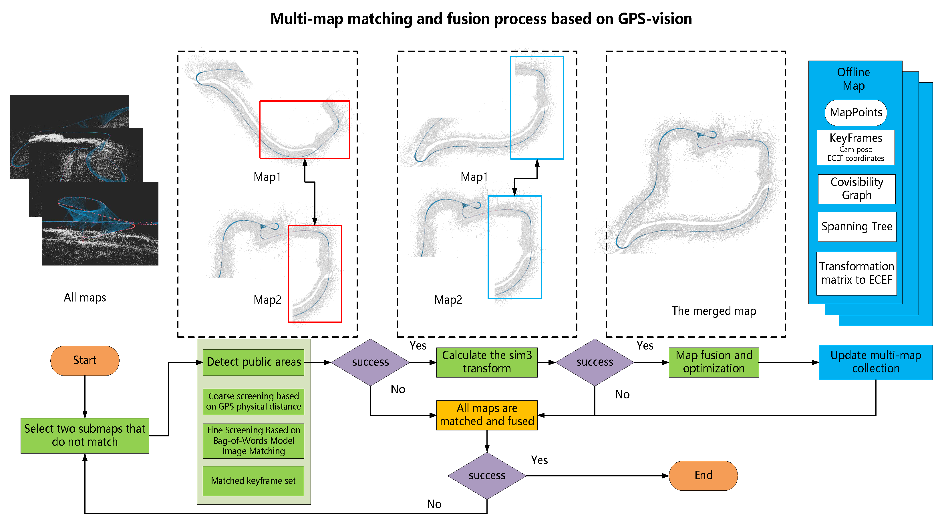
5.2. Multi-Map Merging

Since the data sequence may have an overlapping area at different times, and too many discrete maps cause resource loss and affect location switching, the map management module creates a multi-map fusion strategy to merge the discrete maps with an overlapping area. The specific map merging operation to fuse the current map with the candidate map is shown in Figure 3.

(1) Detection of overlapping areas: The classical visual SLAM often utilizes the bag-of-words model, such as DBOW2, to compute image similarity for detecting overlapping areas. However, this detection method is not robust. Relying solely on visual cues may lead to the failure to detect overlapping areas or even produce erroneous results.

Compared to the commonly used DBOW2 detection in traditional visual SLAM, this paper introduces a GNSS-assisted method for detecting overlapping areas, which greatly enhances the speed and reliability of the detection. This method significantly speeds up the detection process while also reducing the chances of erroneous matches caused by similar scenes. The distance between the current keyframe $\mathcal{X}$ and all keyframes in the candidate map set $\mathcal{M}$ is calculated for the current map, and the nearest candidate map m is obtained as Equation (11), where $\mathrm{g}$ is the GNSS coordinate of the keyframe. The set ${\mathcal{K}}_C$ of the first n nearest candidate fusion keyframes is also preserved in the m map:

$$\mathrm{m}=\underset{\mathrm{m}\in \mathcal{M}}{argmin}{∥\mathrm{g}-{\mathrm{g}}_{\mathrm{i}}∥}_2,{\mathrm{g}}_{\mathrm{i}}\in {\mathrm{m}}_{\mathrm{i}},{\mathrm{m}}_{\mathrm{i}}\in \mathcal{M}$$

(11)

(2) Calculate the sim3 transformation: Traverse all keyframe matching pairs ${\mathcal{K}}_C$ and apply the bag-of-words DBOW2-based image-matching method to obtain the matching relationships between 2D feature points, thus obtaining the matching relationships between 2D points and their corresponding 3D points in the map. Using the ICP algorithm, point cloud registration is performed based on the 3D matching relationships, computing the similarity transformation matrix between the current map and the candidate map as $Q_{est}=sR{t}_{trans}$. During this process, record the candidate keyframe ${\mathcal{X}}_C$ with the highest number of points.

Due to the presence of multiple matching keyframe pairs in set C, it is possible to calculate multiple similarity transformation matrices. Among these calculation results, it is necessary to select the best set to participate in the subsequent computations. First, using $Q_{est}$, the 3D points in keyframe K1 are projected onto the image of keyframe K2. Then, the 3D points in keyframe K2 are projected onto the image of keyframe K1. Subsequently, according to Equation (6), the vector inner product r of the reprojection errors is computed. Further, the inliers and outliers are selected using a threshold based on the chi-square test. Finally, select the keyframe matching pair KF1 and KF2 with the highest number of inliers as representatives of the overlapping area between the two maps, and record the similarity transformation matrix Q calculated based on them.

(3) Map fusion: After computing the overlapping areas between the two maps and the coordinate transformation matrix between the maps, the actual map fusion operation can be performed. Record the current key frame $\mathcal{X}$ and its co-view keyframe as the active co-view window ${\mathcal{W}}_1$, and record the fusion key frame and its co-view keyframe as the fusion co-view window ${\mathcal{W}}_2$. Through the similar transformation relationship $sR{t}_{trans}$ calculated between the two maps, the keyframes and map points of the current common view window ${\mathcal{W}}_1$ are transformed into the candidate map m coordinate system and added to the candidate map. The above process is shown in Equation (12):

$$\begin{array}{c}\hfill T_{update}=sR{t}_{trans}{T}_{origin}\\ \hfill P_{update}=sR{t}_{trans}{P}_{origin}\end{array}$$

(12)

where T represents the position and pose of the keyframe, and P represents the coordinates of the map point.

Using these two co-visual windows, the old map’s spanning tree is merged and updated, and the connections between map points and keyframes are updated to eliminate duplicate map points.

In this paper, the fusion of map points differs from some traditional SLAM methods, as it does not directly use either of the two. Instead of performing a simple replacement, the fusion is weighted based on the weights of each map point, which leads to a more rigorous and effective approach. Specifically, assuming that the map point l is observed in $n_1$ keyframes and the corresponding point $l^{{}^{\prime }}$ is observed in $n_2$ keyframes, the fusion result of l and $l^{{}^{\prime }}$ denoted as $l_{\mathrm{res}}$ is given by Equation (13):

$$l_{res}=\frac{n_{1}l+n_2{l}^{{}^{\prime }}}{n_1+n_2}$$

(13)

Finally, all other keyframes and map points in the current map are transformed and added to the candidate map m to complete the basic map fusion.

(4) Map optimization: In the stitching area, non-linear bundle adjustment (BA) is performed on keyframes and map points in the current frame co-view window ${\mathcal{W}}_1$, while the frames in the fusion co-view window ${\mathcal{W}}_2$ are fixed. Subsequently, a global pose graph optimization is performed to refine the keyframes and map points throughout the entire map.

After the fusion process is complete, the multi-map collection is updated by removing the previous outdated maps and adding the newly merged map. Repeat the above process until the number of maps is reduced to 1, or all maps have been attempted for matching and fusion.

5.3. Multiple Map Switching

When navigating in large-scale environments, even with the assistance of map fusion, relying solely on a single map for visual localization in a planned scene remains highly challenging. For instance, when multiple geographic maps exist involving different temporal and spatial domains, a localization and navigation system needs to possess robust online management and coordination capabilities. Therefore, this paper proposes a multi-map-based visual SLAM online localization system that can effectively localize the scene based on the results of multi-map construction presented earlier. Even in the online motion of unmanned aerial vehicles or ground vehicles, in the event of GNSS data loss, the proposed system can accurately estimate its own position and achieve system relocalization. The experiments demonstrate that the proposed algorithm exhibits higher robustness and accuracy compared to existing SLAM systems.

(1) Map-switching conditions: The switching between multiple maps is based on specific criteria. If the current frame’s localization result is unsatisfactory, the tracking module selects an appropriate map. During the online localization process, the success of the current frame’s pose estimation is determined by the number of tracked map points and the number of inliers in the pose estimation. Additionally, map switching is triggered based on three specific conditions.

Condition 1: During the online relocalization process, if the pose estimation fails for three consecutive frames, it cannot reestablish the localization.

Condition 2: There is no co-vision between the current image and all keyframes on the active map.

Condition 3: The current image is relocalized if its localization accuracy or healthiness does not meet the threshold.

We primarily rely on Condition 1 and Condition 2 for determination. In our assumed working scenario, UAVs and eVTOL experience long periods of GNSS signal interference and loss while performing transportation tasks within mapped areas. Therefore, real-time localization heavily relies on purely visual methods. In any of the situations above, a multi-map switching operation is triggered, leading to the abandonment of the current map and the selection of a new map to facilitate subsequent localization tasks. Condition 3 is only utilized in ideal scenarios with good GNSS signal conditions. The best localization results can be achieved by combining reliable GNSS signals and visual maps. The visual relocalization accuracy is evaluated based on the current real-time GNSS information. This condition can be used to assess the reusability of existing maps and further determine whether to update historical maps or add new map sets.

(2) Map-switching algorithm: During the offline automatic construction of multiple maps, all keyframes, 3D points, transformation matrices to the world coordinate system, and other relevant information in the maps are recorded. This paper provides grid-based map information for the offline map workspace based on these conditions. This information records the distribution of all maps within the entire map scene. First, the unmanned aerial or ground vehicle’s working area is defined as a large rectangle. The GNSS with the strongest satellite positioning system signal among all keyframes is chosen as the origin of the grid coordinate system. The longitude is assigned to the y-axis, and the latitude is to the x-axis. We set the size of each small square as 700 × 700 m (precisely adjusted based on the size of the mission area and onboard equipment resources). By utilizing the conversion relationship between meters and latitude/longitude, we can determine the actual latitude and longitude values for each grid in the map. Next, based on the GNSS with the strongest signal among the keyframes, the number of squares in the longitude and latitude directions can be calculated and numbered starting from 0. Finally, we can determine their corresponding coordinates on the grid map using the GNSS positions of each keyframe on the map. This allows us to obtain a list of maps for each grid.

During the initialization process, the online relocalization system will load all the offline constructed multi-map grid information. When the UAV or ground vehicle triggers the map-switching conditions described earlier during its motion, the system will automatically initiate the map-switching algorithm. When selecting the candidate map for switching, the system will prioritize the principle of minimum distance. If the current frame fails to localize, the system will use the pose result from the previous frame as the current localization position. Then, it will search for the candidate map with the closest physical distance to the current situation in the candidate map collection and switch to using that map. Specifically, the estimated pose $(x,y,z)$ of the previous frame is converted into the ECEF coordinate system through the transformation matrix of the current map, and the calculation formula is as follows:

$$\begin{array}{c}\hfill \left[\begin{array}{c}X\hfill \\ Y\hfill \\ Z\hfill \\ W\hfill \end{array}\right]=\left[\begin{array}{cc}sR& t\\ 0& 1\end{array}\right]\left[\begin{array}{c}x\hfill \\ y\hfill \\ z\hfill \\ 1\hfill \end{array}\right]\\ \hfill pos{e}_{ecef}=(\frac{X}{W},\frac{Y}{W},\frac{Z}{W})\end{array}$$

(14)

where s, R and t represent the scaling factor from the model coordinate system to the ECEF coordinate system, 3 × 3 rotation matrix and 3 × 1 translation vector, then the position coordinates $(x,y)$ of the current UAV or vehicle in the grid coordinate system are

$$\left\{\begin{array}{c}x=\frac{cu{r}_x-or{i}_x}{\left|dx\right|}\hfill \\ y=\frac{cu{r}_y-or{i}_y}{\left|dy\right|}\hfill \end{array}\right.$$

(15)

where $(cu{r}_x,cu{r}_y)$ is $pos{e}_{ecef}$, which corresponds to the position under the GNSS coordinate system, while $(or{i}_x,or{i}_y)$ is the GNSS coordinates of the grid coordinate system origin. $dx$ and $dy$ represent the scale of a grid in the x and y directions, respectively.

Then, according to the current coordinates, all maps in the four fields above, below, left and right of the grid are obtained to generate an Atlas. The current GNSS and the GNSS of all keyframes in each map are used to calculate the Euclidean distance, and the Atlas is sorted from near to far. A new map is selected from the sequence when a map is switched.

Additionally, we designed a criterion to determine the success of map switching. After the switch, continuous successful localization across multiple frames is required within the switched map to confirm a successful switch. Lastly, the system outputs the current UAV or ground vehicle’s valid position and attitude information to the control terminal.

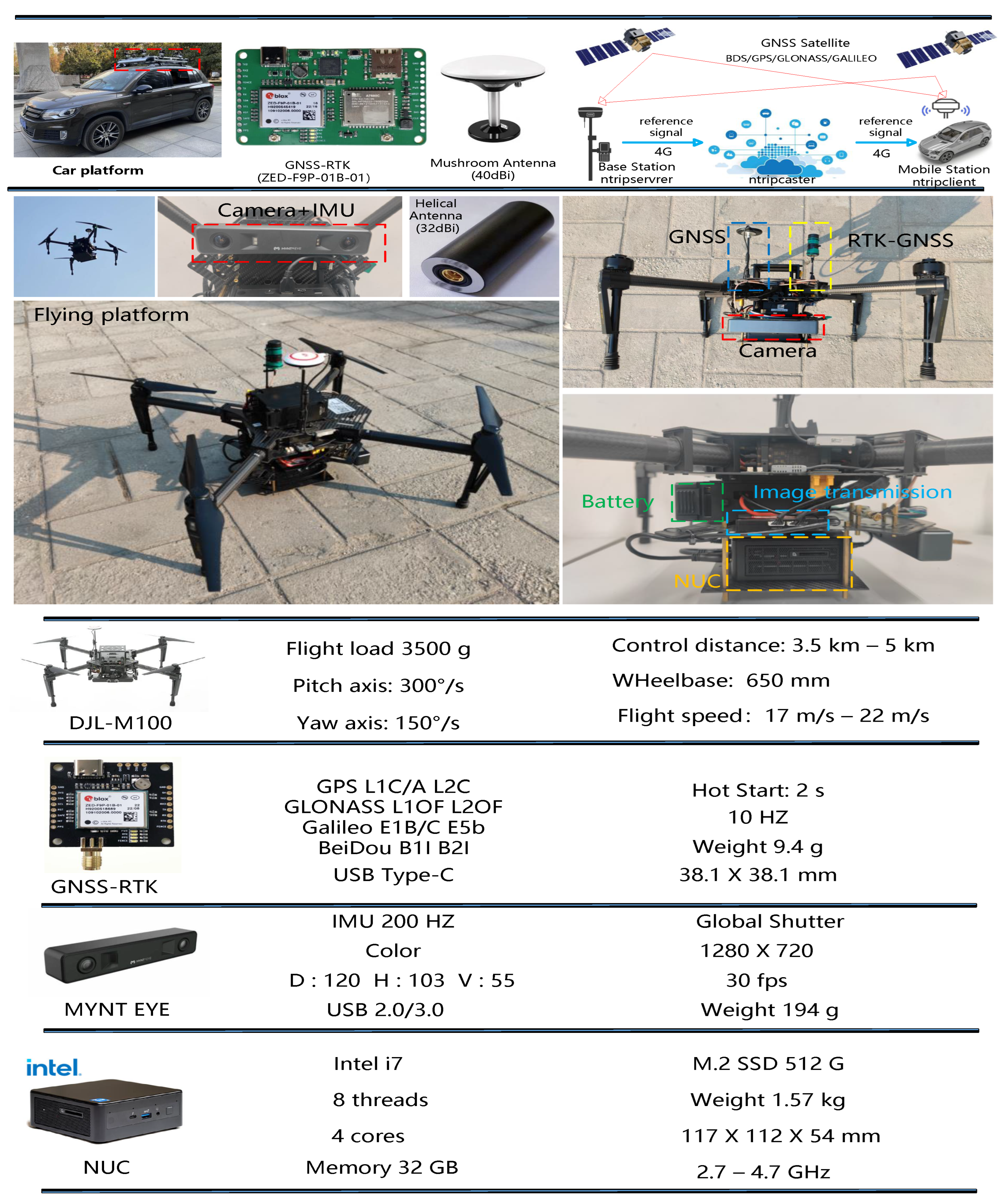
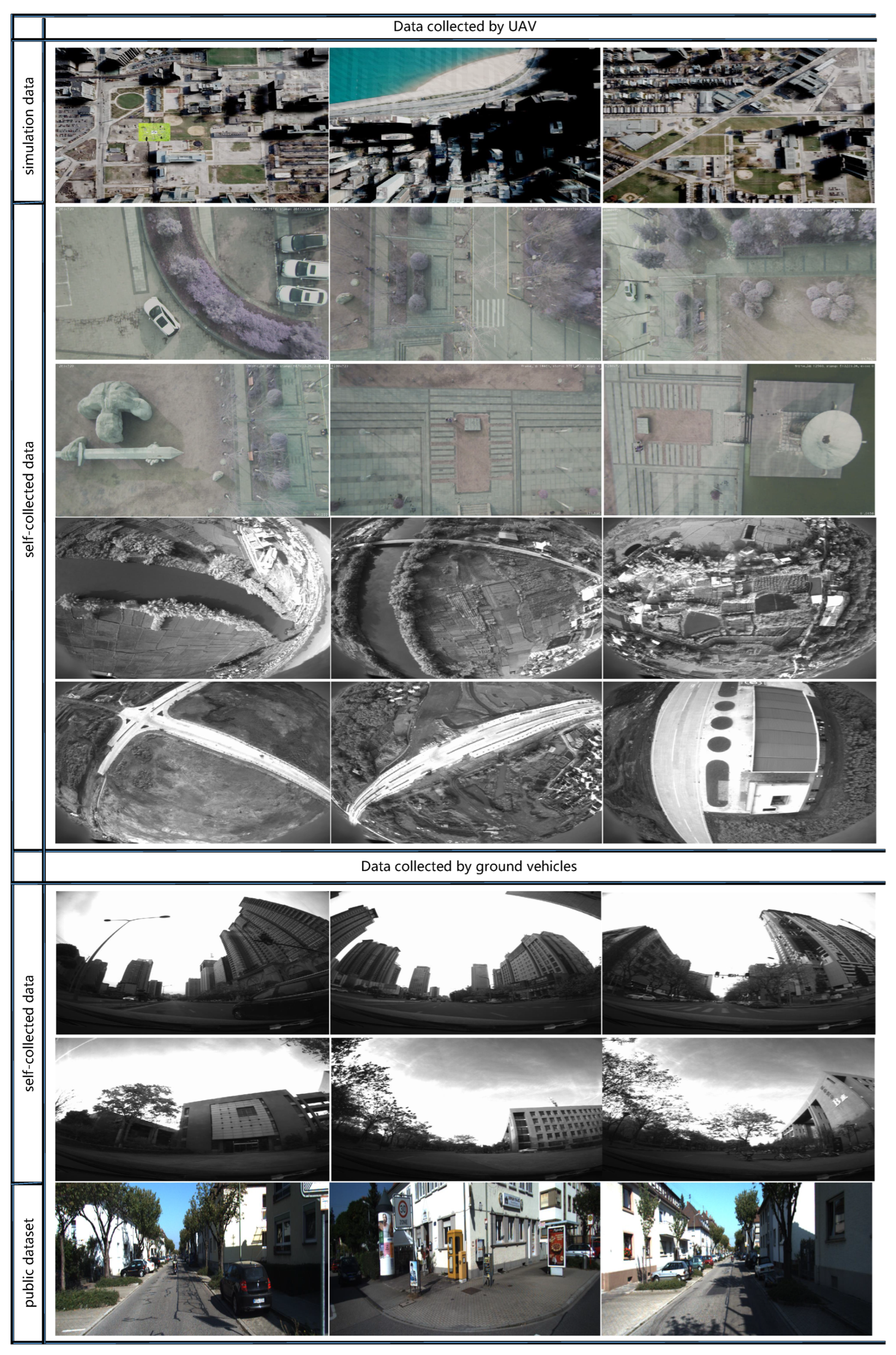
6. Experimental Results

We evaluate the proposed system utilizing both real-world trials and aerial simulation datasets. Then we construct a real LD-SLAM system that includes a fisheye camera, GNSS, and an Intel NUC tiny PC. The specific information on the experimental equipment is shown in Figure 4. Comprising UE4 and Airsim, we first generate an aerial dataset with sceneries of towns, villages, roads, rivers, etc. The dataset used is shown in Figure 5. In our experiment, we deploy the system on drones and ground vehicles to assess its performance in a distant outdoor space. Finally, we investigate and discuss the system’s overall processing speed as well as the duration of each component’s calculations. The precision, robustness and efficiency of our technology are clearly shown by the quantity and quality analyses.

The selected multi-frequency GNSS receiver model used in the experiment is the ZED-F9P module, which is a 4-constellation GNSS system capable of simultaneously receiving GPS, GLONASS, Galileo, and BeiDou navigation signals. When combined with an RTK base station, it achieves centimeter-level accuracy within seconds. The RTK system provides various types of positioning, including “NARROW-INT” (a multi-frequency RTK solution that resolves narrow lane integer carrier phase ambiguities), “PSRDIFF” (a solution calculated with differential pseudo-range corrections using DGPS or DGNSS), and “SINGLE” (a solution computed solely using data provided by GNSS satellites). The compact and energy-efficient nature of this module makes it suitable for deployment on UAVs. It exhibits short convergence time and reliable performance, providing a fast update rate for high dynamic application scenarios. All sensors are synchronized with the GNSS time through hardware triggering. The specific parameters are shown in the Figure 4. Before integrating GNSS information into sensor fusion systems, it is necessary to perform a preliminary detection of outlier states. Failure to do so may result in reduced accuracy due to erroneous GNSS information. GNSS measurements include information such as receiver status, number of satellites, position dilution of precision (PDOP), and the covariance matrix of the positioning results. The provided information can be used for the initial filtering of GNSS measurements to eliminate abnormal frames. On the one hand, adding a constraint to the starting point position ensures better quality of the GNSS data collected. On the other hand, accumulating a sufficient amount of high-quality GNSS points and performing batch optimization is essential to achieve the alignment of GPS and SLAM trajectories in one step. By utilizing a high-precision visual map established with the assistance of GNSS, the proposed system can provide accurate, robust, and seamless localization estimates along the entire trajectory, even in long-term GNSS-obstructed conditions.

The reliability of GNSS is compromised within urban canyons or tunnels. We only consider the reference pose when GNSS is available and the standard deviation of the observed position is small. An outlier processing algorithm is applied to the data from visual and GNSS observations to enhance the system’s robustness, particularly in complex environments. GNSS anomaly detection enables the identification of faults in GNSS signals, ensuring that anomalous GNSS positioning outcomes do not impact the entirety of the trajectory. For the GNSS raw data, we exclude satellites with low elevation angles and those in an unhealthy state, as these satellites are prone to introducing errors. To reject unstable satellite signals, only those satellites that maintain a continuous lock for a certain number of epochs are permitted to enter the system.

For future convenience in understanding, we established several symbols and terms.

• VO Map: The map was built using only visual information without GNSS optimization.
• VO + GNSS Map: The map was constructed by fusing data from multiple sensors, including visual and GNSS information.
• VO Localization: The pose estimation was conducted solely using visual odometry without GNSS optimization.
• VO + GNSS Localization: The pose estimation was optimized using the joint information of visual odometry and GNSS.

To validate our algorithm’s performance, we conducted relocalization experiments in three distinct environments: virtual simulations, real-world unmanned aerial vehicle flights, and real-world ground vehicle operations. These will be presented in the following three subsections: A, B, and C. We conducted three separate sets of controlled experiments in each experimental setting to validate the performance of our algorithm in multiple modes fully. The three experimental conditions are shown below:

The first mode (VO Map—VO Localization) utilizes pure vision to perform relocalization on a map built purely of visual information. In scenarios of long-range navigation (e.g., flying for tens of kilometers), this mode serves as a fundamental benchmark for localization comparison due to the accumulation of errors caused by the lack of global optimization assistance.

In the second mode (VO + GNSS Map − VO + GNSS Localization), GNSS signals are utilized for optimization in both map generation and online localization stages. This model is the most optimal working solution since GNSS signals are of good quality during the online localization phase, allowing continuous participation in localization optimization. Moreover, the employed high-precision map fuses global positioning information for improved accuracy. Unfortunately, the electromagnetic environment is complex and variable, and GNSS signals may be lost for a long time. Malicious interference with GNSS signals may occur for some important safety applications, leading to the unavailability of global positioning information.

In the third mode (VO + GNSS Map − VO Localization), pure visual relocalization is performed using a high-precision map optimized with GNSS data. This mode closely matches real-world application scenarios. In some fixed use cases, such as unmanned aerial vehicle logistics, a high-precision map can be constructed in advance under the premise of good GNSS signals. During online use, pure visual localization is primarily used, and global positioning information can be obtained using an offline map regardless of the quality of GNSS signals.

We utilize GNSS-RTK data as a reference for the ground truth trajectory. In long-range navigation tasks, the traditional visual localization method, which solely relies on loop closure detection and global BA, cannot effectively reduce cumulative error, as evidenced by the experimental comparison of Patterns 1 and 3. However, incorporating GNSS global information into a multi-sensor data fusion-based localization method can effectively address this issue. Through the experimental comparison of Patterns 2 and 3, we find that the accuracy of high-precision map-based localization optimized with GNSS assistance is comparable to that of GNSS localization. The experimental results for this section are presented in

Table 1. The final root mean square error (RMSE) of each approach.

RMSE IN MAP EXPERIMENT.
Sequence	Length (km)	Proposed RMSE (m)
		VO Map		VO + GNSS Map
FlySImulation-Data1	58.991	2.727		0.907
FlyReal-Data1	31.542	13.274		0.838
CarReal-Data1	4.986	5.51		0.655
RMSE IN LOCALIZATION EXPERIMENT.
Sequence	Length (km)	Proposed RMSE (m)
		VO Map VO Localization	VO + GNSS Map VO Localization	VO + GNSS Map VO + GNSS Localization
FlySImulation-Data2	3.14	4.69	2.232	0.919
FlyReal-Data2	9.94	15.59	3.043	2.431
FlyReal-Data3	16.8	12.728	2.962	2.502
CarReal-Data2	1.35	16.334	2.204	2.116

.

A.

Simulation Environment: Chicago Scene Data

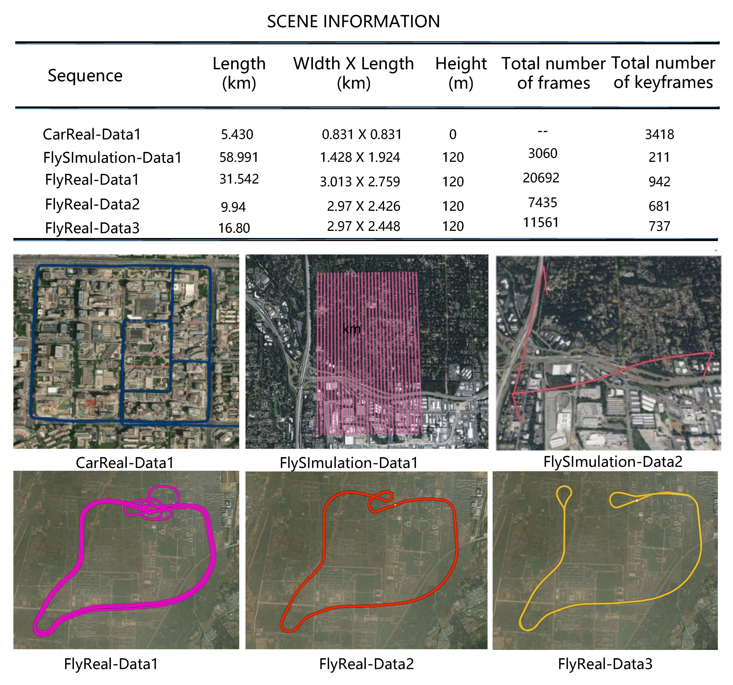
Mapping data: We use Unreal Engine 4 to create a Chicago city simulation scene in a virtual environment and use Airsim to simulate the drone collecting images and GNSS data in strips over the city, which includes three takeoff and landing sites. The drone has a flight altitude of 200 m, a bandwidth of 1.420 km, a band length of 1.924 km, a total mileage of 58.991 km, and a frame rate of 10 frames per second. For each image in this dataset, there is ground truth for the drone’s position, attitude, and GNSS, and the total number of aerial images is over 20,000.

Localization data: In the area of the mapping data, the drone flies in a curve. The flight altitude is 200 m, and the total flight distance is 31.43 km.

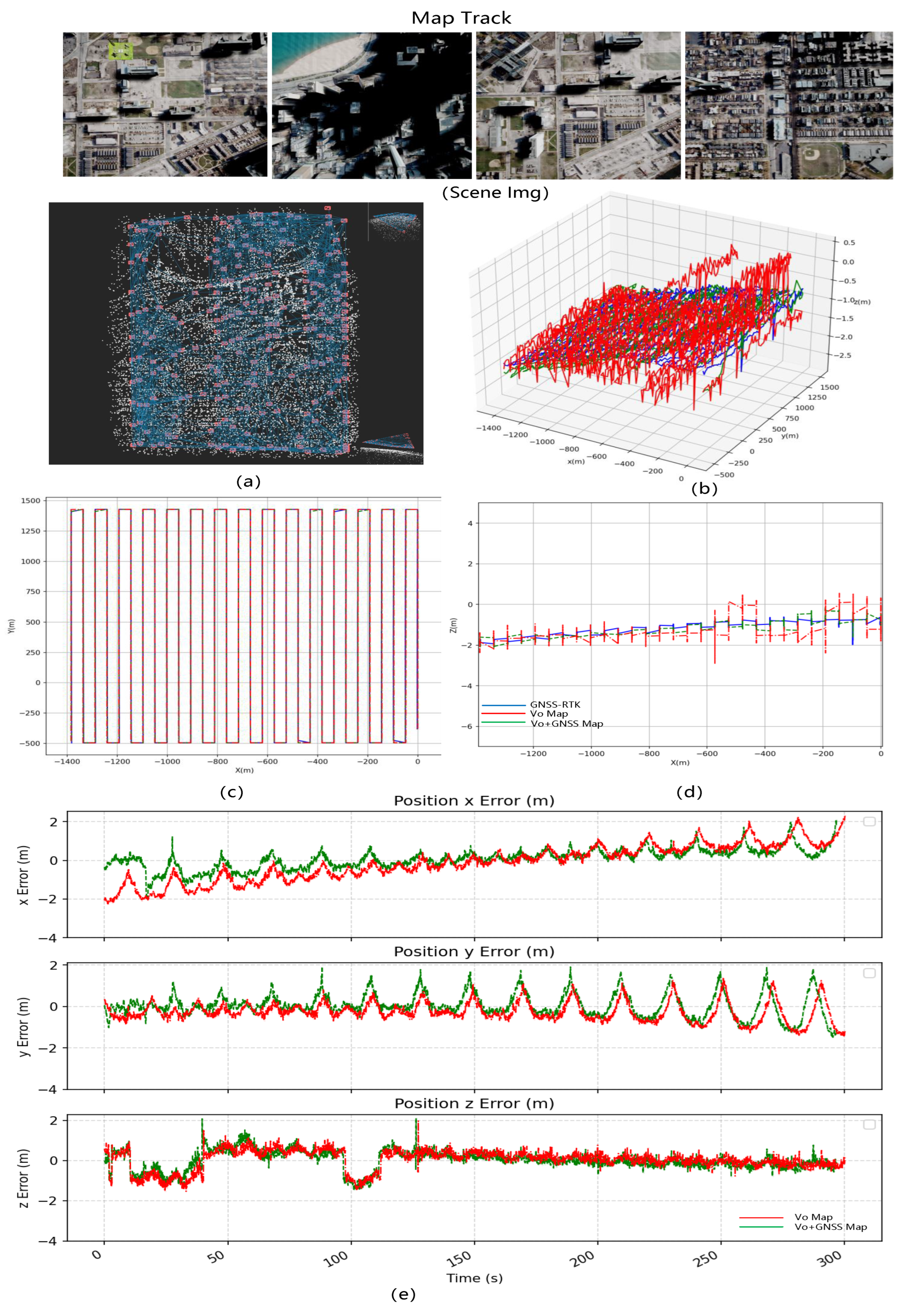
LD-SLAM Result: We use the mapping data to build the map in two modes: pure vision SLAM and vision + GNSS optimization, draw the trajectory and compare the error by converting the calculated value and real GNSS to ECEF coordinate system. Figure 6 shows the mapping data with Figure 6a the point cloud map, Figure 6b the trajectory of the mapping results and Figure 6c–e the error comparison between the visual SLAM mapping results and the visual+GNSS optimized mapping results. The trajectory figure shows that the z-direction of flight varies significantly under purely visual SLAM. After adding the GNSS optimization, the jitter decreases, and the trajectory approaches the true value. The total error of the three XYZ directions is 0.2 to 0.3 m smaller.

Using the aforementioned mapping data, we created two maps—the VO map and the VO + GNSS map—which will be used in subsequent relocation experiments. In the simulation test environment, we observed an overall root mean square error (RMSE) of 4.69 m in Pattern 1 (VO Map − VO Localization), with no greater deviation due to the dense strip-shaped flight trajectory that is conducive to visual mapping and localization. In Pattern 2 (VO + GNSS Map − VO Localization), the relocation accuracy improved to 2.232 m, thanks to the use of GNSS assistance that improved the accuracy of the visual map. In Pattern 3 (VO + GNSS Map − VO + GNSS Localization), the relocation accuracy further improved to 0.919 m, undoubtedly due to the excellent GNSS global information assistance for both the mapping and online visual localization optimization. Although Pattern 3 is the optimal pattern, we must consider the possibility of long-term GNSS loss in practical situations. Therefore, in practice, Pattern 2 will be used in most cases. Figure 7 shows the results. The error curve shows that the position accuracy of the optimized map with GNSS is superior to the purely visual map in terms of longitude and latitude errors. Figure 7 shows that after adding the GNSS optimization, the error in the xy direction break is 1 to 2 m less than just what is seen.

B.

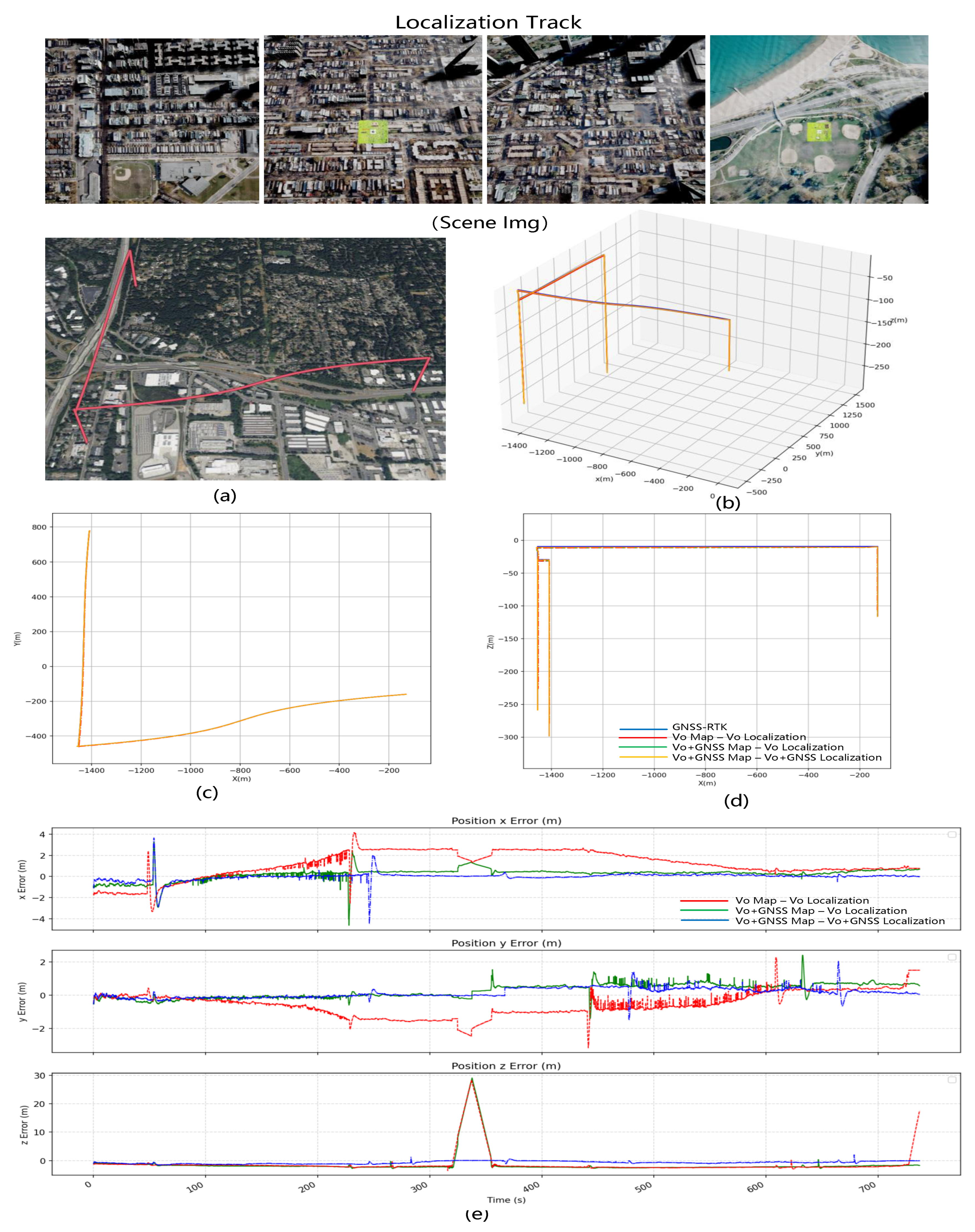
Real Scene UAV Aerial Photography Data

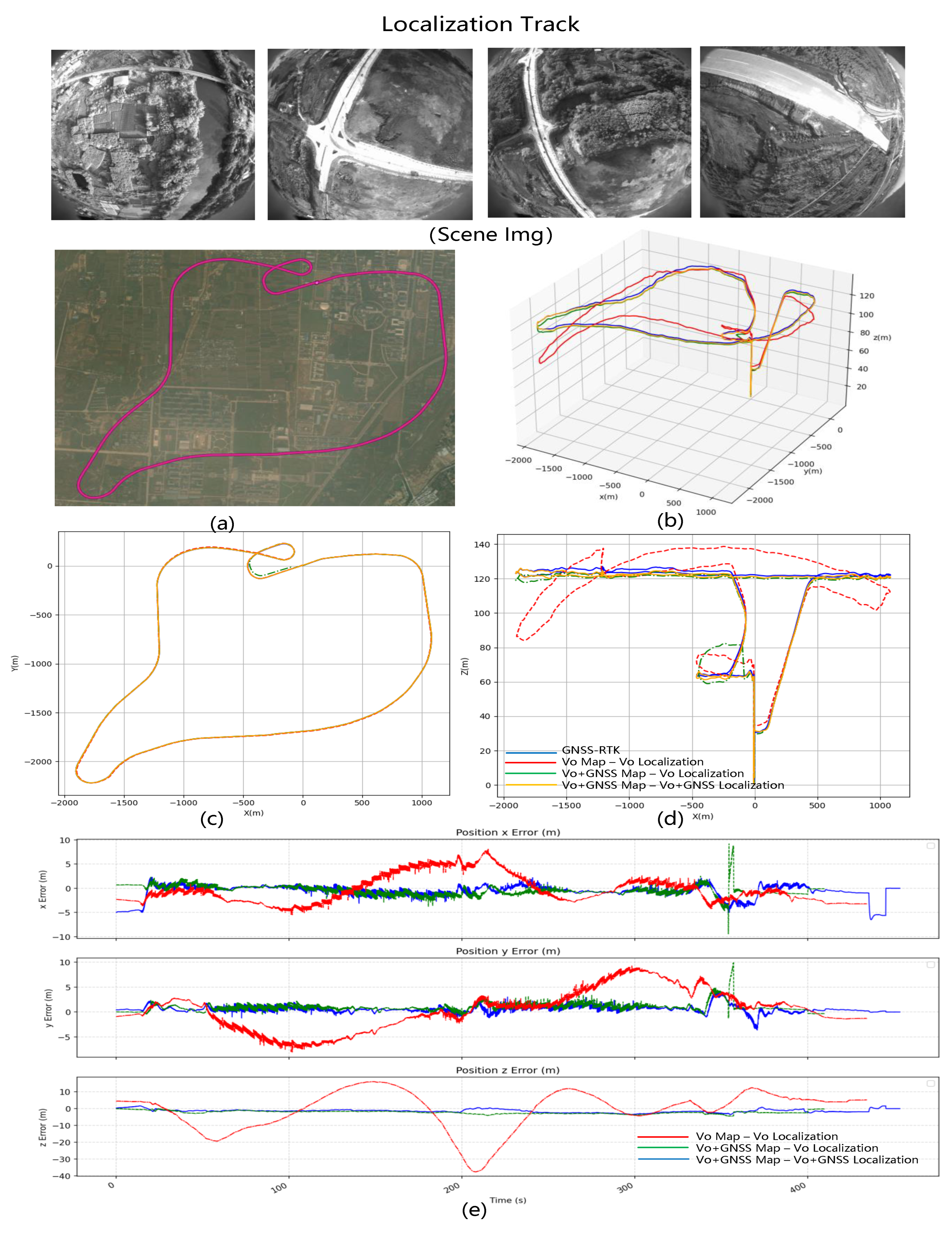
Mapping data FlyReal-Data1: We use a drone to capture multiple sets of data in the normal environment. The trajectory of the drone is shown in Figure 8. The flight altitude is 120 m, the total mileage is 31.54 km, the frame rate of image acquisition is 15 frames, and the frame rate of GNSS acquisition is 10 frames.

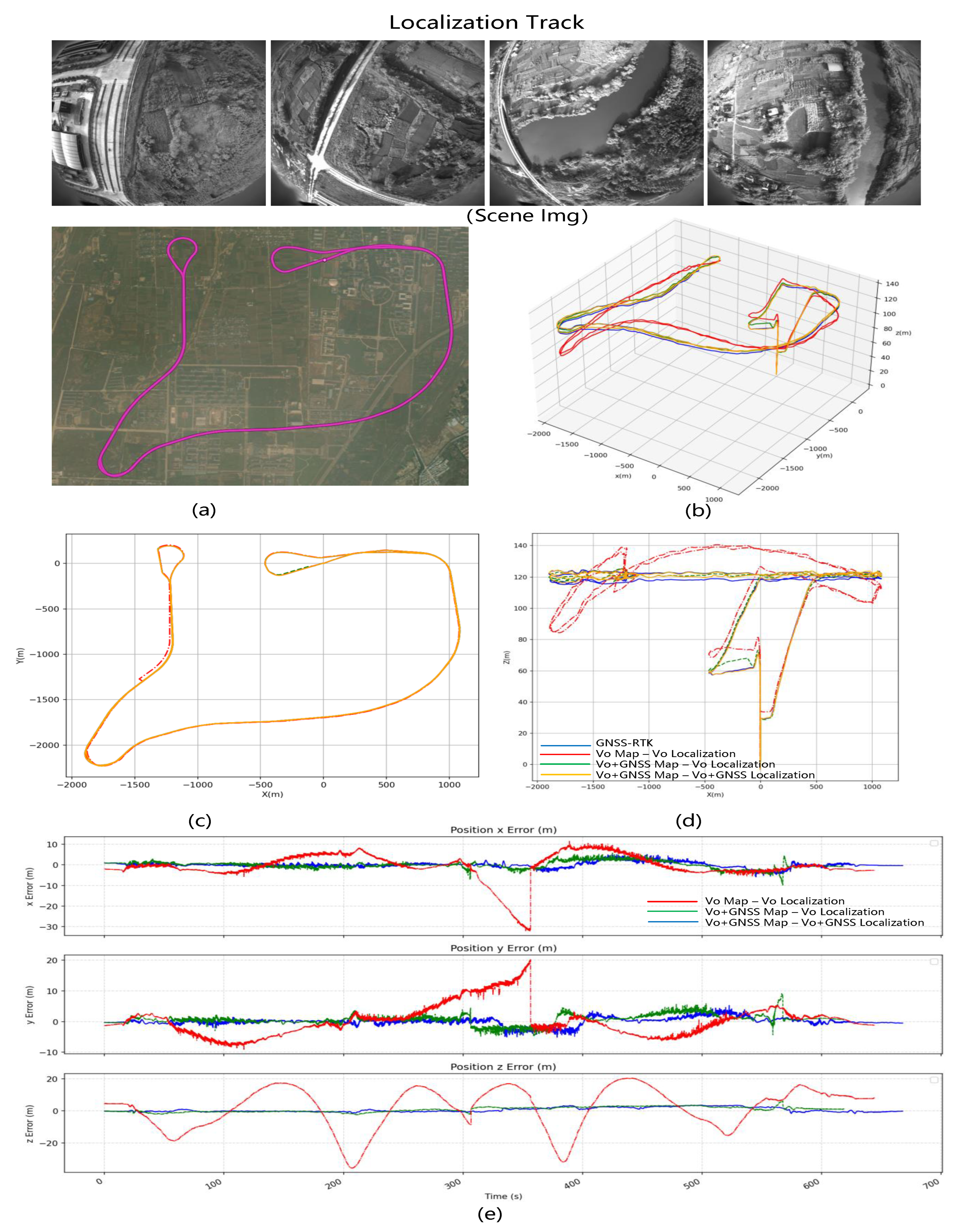
Localization data FlyReal-Data2: Within the same scene, the drone flies back and forth according to the mapping data track. The specific trace is shown in Figure 9. The flight altitude is 120 m, the total mileage is 16.808 km, the frame rate of image acquisition is 15 frames, and the frame rate of GNSS acquisition is 10 frames.

Localization data FlyReal-Data3: We fly a circle in the mapping scene x according to the mapping track. Figure 10 shows the specific lane. The flight altitude is 120 m, the total mileage is 9.945 km, the frame rate of image acquisition is 15 frames per second, and the frame rate of GNSS acquisition is 10 frames per second.

LD-SLAM Result: Similar to the Chicago experiment, we created maps for both the Vision + GNSS Optimization and Pure Vision Slam modes using this dataset, as shown in Figure 8. Since an actual drone captured this dataset, the results are more convincing than those obtained with simulated data. In the simulation scenario, the flight path was changed from an ideal strip to a multi-layer circular long-distance path with varying elevations. The purely visual elevation gain error fluctuation was clearly visible in the real long-distance data, with the error reaching up to 30 m. After GNSS optimization, the error in all three directions was reduced to within 1 m.

We conducted three experimental groups utilizing the FlyReal-Data2 test dataset, similar to the Chicago experiment. Test results are shown in Figure 9. The location results obtained with maps after GNSS optimization are significantly better than those obtained using the pure Vision Slam. In vision-only mode, errors in the XYZ direction can reach up to 30 m, whereas GNSS optimization can often reduce errors in all three directions to within 2 m. The pure vision error map has a sudden increase in error due to the UAV flying out of the map during testing. Due to the tendency for errors to accumulate during SLAM turning without GNSS optimization, errors can rapidly grow and exceed 30 m in a short amount of time. The system will start repositioning and create sharp increases in errors when significant errors occur. With GNSS optimization, the UAV error after leaving the mapped region is always within 2 m, and it can maintain a high level of accuracy without requiring loopback data.

Figure 10 shows similarities between the FlyReal-Data3 test results and the previously discussed results. Applying GNSS optimization leads to improved positioning accuracy, particularly at higher altitudes. In pure visual mode, errors in the xy direction can reach up to 5 m; in the z-direction, errors can be as high as 30 m. However, after applying GNSS optimization, errors in all three directions are often reduced to within 2 m. The drone flew beyond the map’s limits in some parts of the middle and rear sections. Our method can accurately track and relocate the drone, even under challenging circumstances such as flying out of the map’s limits.

These experiments further validate the reliability of our system in real-world scenarios. During the 16 km long-distance flight relocalization test, the precision error difference between mode 2 (VO + GNSS Map − VO + GNSS Localization) and mode 3 (VO + GNSS Map − VO + GNSS Localization) was only around 0.5 m. This fully demonstrates the effectiveness of the maps optimized with GNSS assistance. For multi-rotor aircraft performing tasks, such as the delivery and transport of people, it is possible to construct high-precision offline maps in advance within the flight mission area when the GNSS signal is strong. When the GNSS signal is lost due to malicious interference, high-precision offline maps can provide global positioning information to replace GNSS.

C.

Real Scene Ground Vehicle Data

Our ground dataset was collected by a modified SUV in intricate urban settings, with the vehicle reaching a maximum speed of approximately 15 m per second during the data acquisition process, as shown in Figure 4. The road where the collection took place is flanked by tall buildings spanning several tens of meters, with the heights of these high-rise mainstream structures ranging from 150 to 250 m. Near the central garden square in the city center, there is a circular road surrounded by towering skyscrapers, highly convenient transportation, and some dynamic objects present. Additionally, data are collected by driving on elevated bridge roads within the urban area. These structures serve as prominent landmarks, facilitating the extraction of visual features. During collection, the vehicle will pass through several traffic light intersections, typically maintaining a certain distance from the preceding vehicles. Rapid passage beneath elevated bridges may occasionally temporarily degrade GNSS signals for a few seconds. Therefore, outlier processing algorithms are applied to the data from visual and GNSS observations to enhance the system’s robustness, particularly in complex environments.

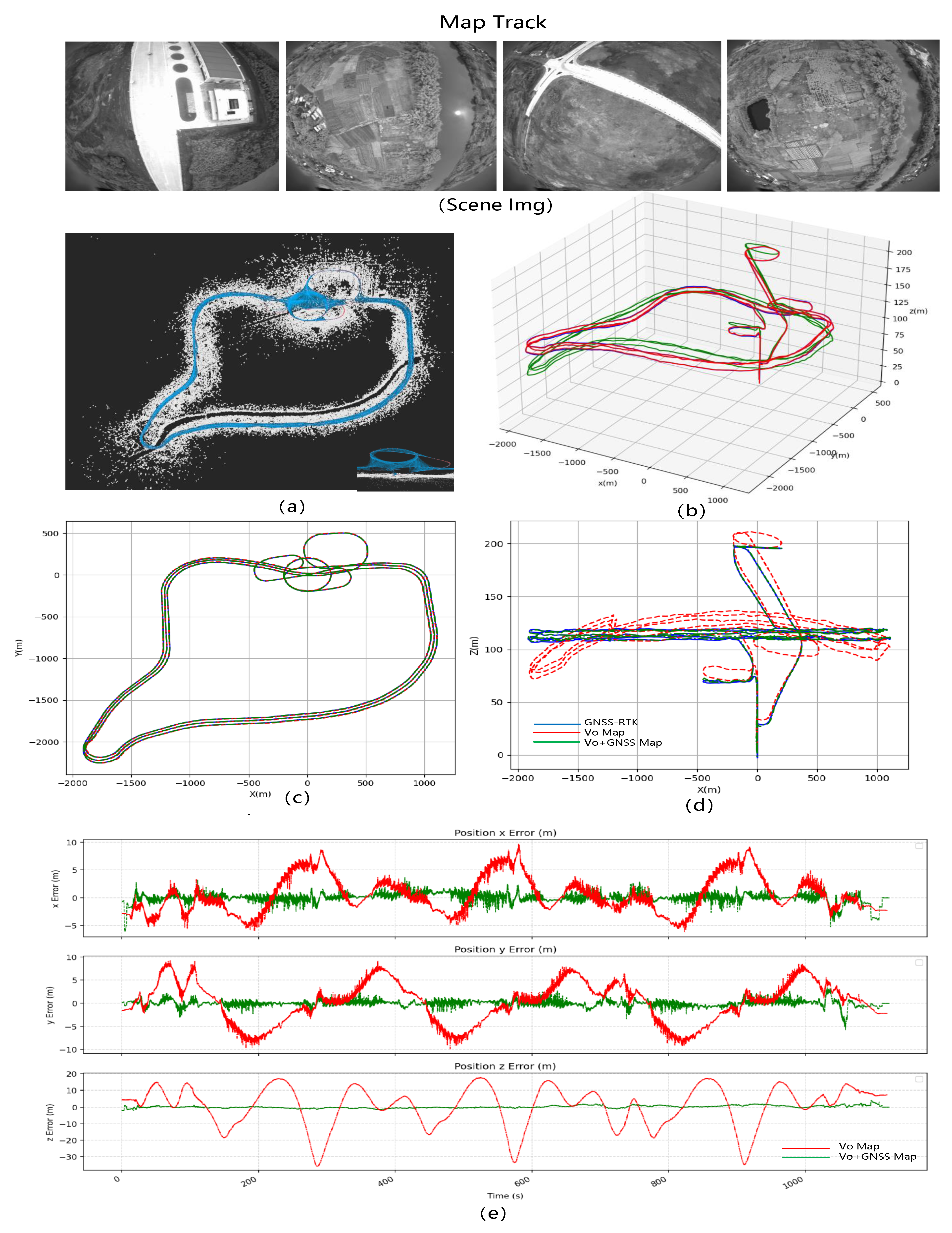
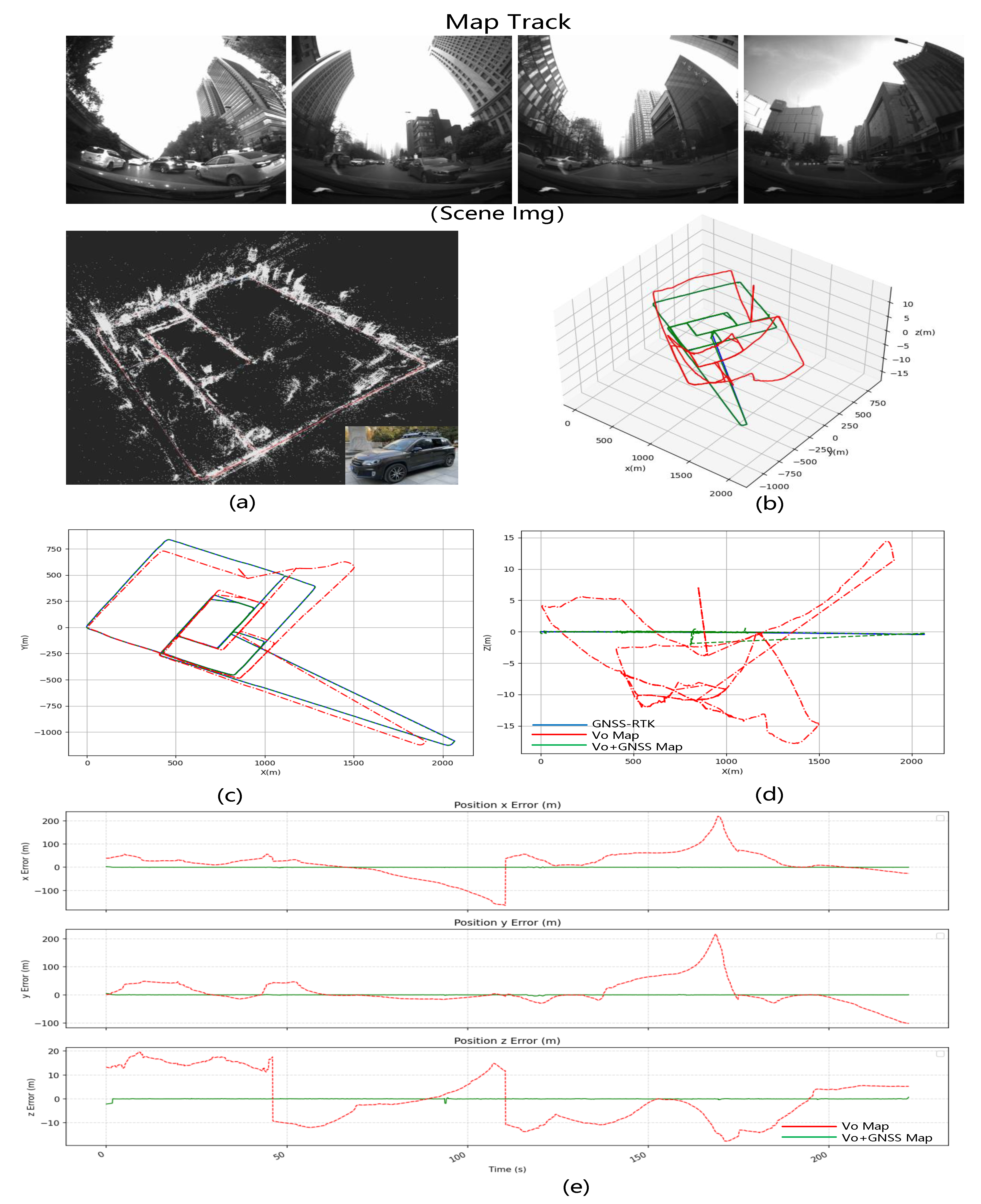
Mapping data: Install our SLAM system on the ground vehicle and collect data on the road with the front fisheye camera. Figure 11 shows the vehicle run distance with a total mileage of 5.430 km, a frame rate of 15 and a GNSS frame rate of 10.

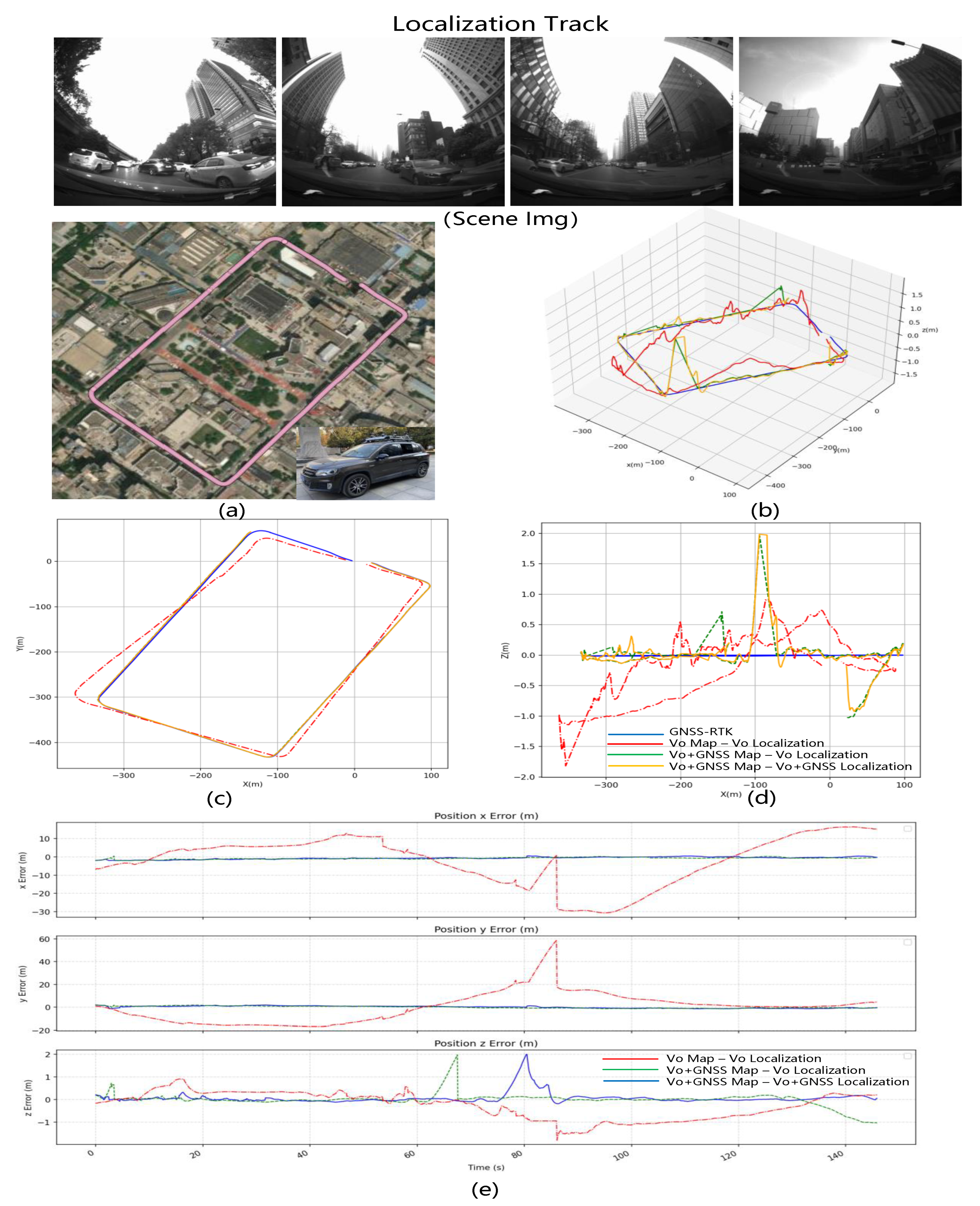
Localization data: The vehicle moves through the city blocks in the test data. Figure 12 shows the vehicle route. The vehicle’s total mileage is 2.318 km, the frame rate is 15, and the GNSS frame rate is 10.

LD-SLAM Result: Two mapping modes are utilized for ground data: pure vision SLAM and vision + GNSS optimization as shown in Figure 11. Ground imagery poses more complex analysis conditions than aerial imagery due to factors such as lower texture, poor illumination, and accumulation errors. In pure vision, the turning scale is significant. Pure vision typically employs loopback to correct scale drift and cumulative errors. However, the loopback’s global BA optimization is time-consuming and produces an unstable optimized result for long-distance driving and fewer feature points extracted from the image. For instance, in the pure visual mode of Table 1, the original square trace becomes irregular due to the loopback optimization, drastically decreasing the overall accuracy.

Three experimental groups were conducted similarly to Chicago using test data. Figure 12 shows the test results. The GNSS-optimized map positioning results are significantly better than pure vision SLAM. Due to the complex and changeable environment, in the pure visual mode, the error in the two directions of xy can be as high as 30 m, the overall trajectory is offset, and the error remains within 1 m after adding GNSS optimization, which shows that our system still has good robustness in the complex environment of high exposure and multiple moving objects.

An additional advantage of these visual maps is their dynamic updating capability while maintaining accuracy. During each unmanned aerial vehicle’s operation within the same region, updated visual positioning information is integrated into the previous map to improve the accuracy of subsequent UAV relocalization. Multiple visual maps can be constructed at different times in the same area to improve relocalization accuracy. Thus, it becomes favorable in addressing complex illumination changes, particularly seasonal variation that results in significant texture changes.

The final root mean square error (RMSE) of each approach is shown in Table 1.

D.

Multi-algorithm Comparison Experiment

In order to further compare the excellent performance of the algorithm, we selected ORB-SLAM3, Openvslam, and Vins-Fusion, three advanced algorithms, for comparison. Among them, Openvslam and ORB-SLAM3 are pure monocular vision SLAM systems, and Vins-Fusion is a SLAM system that uses GNSS to participate in optimization. VINS-Fusion is a multi-sensor state estimator that operates based on optimization principles. VINS-Fusion supports four types of visual-inertial sensors: monocular camera + IMU, binocular camera + IMU, binocular camera only, and binocular camera + GNSS. In our study, we specifically focus on the joint-optimized positioning of visual odometry (VO) and GNSS. Therefore, we selected the binocular camera + GNSS working mode of VINS-Fusion for comparison.

In order to ensure the integrity of the experiment, we selected three typical long-distance aerial photography datasets in the air. We compared the root mean square errors of the four algorithms in each scenario and visualized the 3D trajectory and the error trend of the trajectory in each direction. By comparing with Openvslam and ORB-SLAM3 monocular pure vision SLAM systems, it highlights the advantages of SLAM systems optimized with GNSS in long-distance visual navigation, which can greatly reduce the cumulative error of vision and improve the accuracy of positioning. By comparing with the Vins-Fusion algorithm, the experiment shows that our algorithm works stably and has higher accuracy in the same GNSS-optimized SLAM system, especially in the face of long-distance cumulative errors, large-scale rotation of viewing angles, high-level jumps, and other complex positioning problems.

Table 2. The RSME of the data comparison of the four algorithms.

RMSE IN OUTDOOR EXPERIMENT.
Sequence	Length (km)	Proposed RMSE (m)
		OPENVSALM Monocular	ORB-SLAM3 Monocular	VINS-FUSION Stereo + GNSS	LD-SLAM Monocular + GNSS
FlyReal-Data1	31.54	46.041	19.827	5.829	0.838
FlyReal-Data2	9.94	26.863	12.416	1.631	1.601
FlyReal-Data3	16.8	24.196	11.919	0.501	0.44

shows the average root error of the four algorithms under three sets of data.

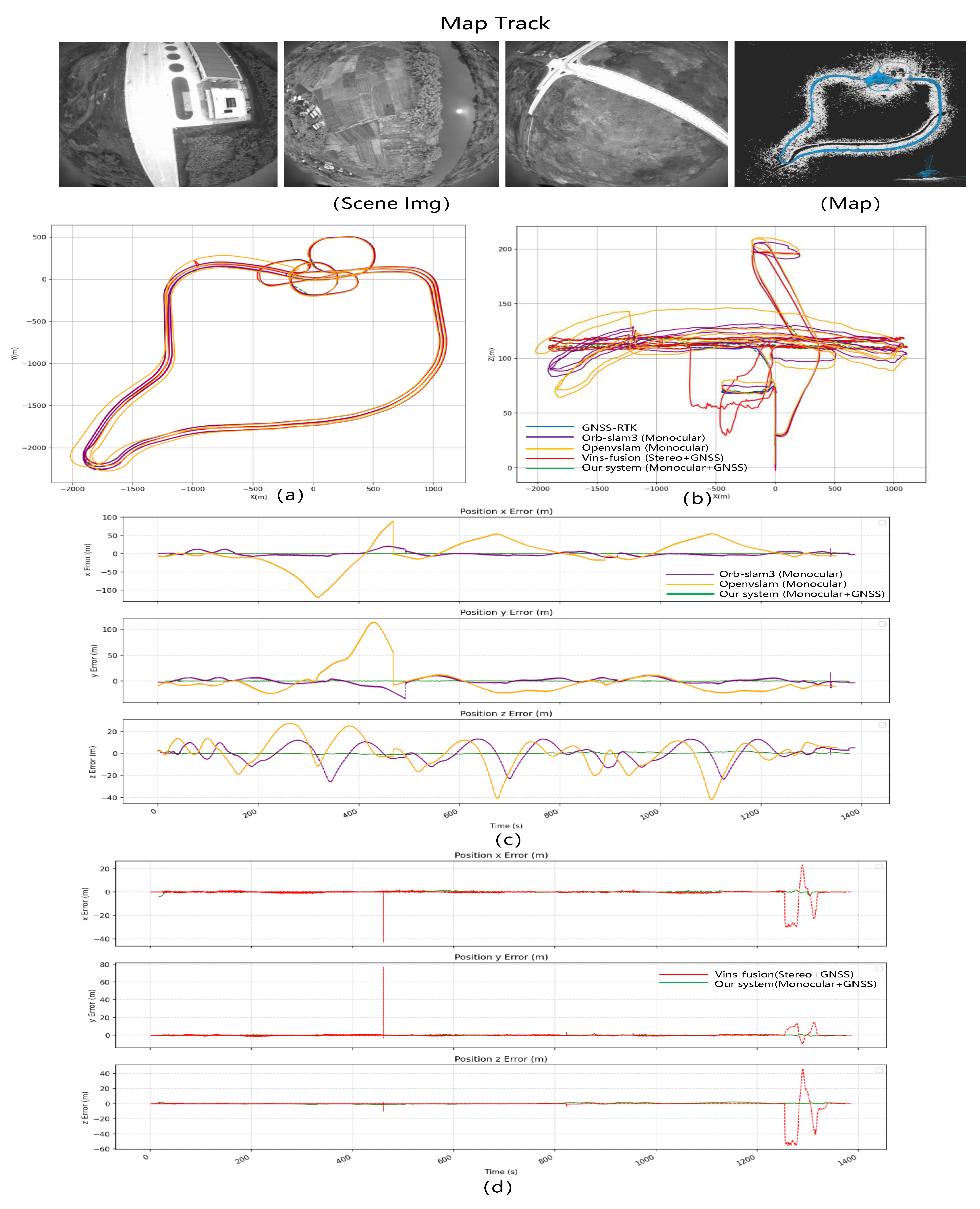
(1) Real-scene data FlyReal-Data1 Comparative Experiment

Mapping data FlyReal-Data1: We use a drone to capture multiple sets of data in the normal environment. The trajectory of the drone is shown in Figure 13. The flight altitude is 110 m, the total mileage is 31.54 km, the frame rate of image acquisition is 15 frames, and the frame rate of GNSS acquisition is 10 frames.

Compare Results: Among the three test scenarios, this set of data is for the longest flight distance. For the monocular pure vision SLAM system, the cumulative error is the largest. In the turning part of the flight path, the camera shooting angle changes too much following the rotation of the drone, resulting in serious deviations in pure visual positioning. From the trajectory diagram in the lower left corner of Figure 13a, it can be seen that the monocular vision Openvslam pose prediction seriously deviates from the actual track. From the trajectory diagram in the middle part of Figure 13b, it can be seen that Openvslam and ORB-SLAM3 have serious fluctuations in the pose estimation of height, especially in the turning stage. The limitation of the monocular vision SLAM system causes the pose estimation to seriously deviate from the actual position when turning and height changes and is accompanied by long-term cumulative errors. Finally, the RMSE of Openvslam and ORB-SLAM3 is 46.041 m and 19.827 m. In the case of long-distance visual navigation, after using GNSS data fusion, our algorithm and VINS-fusion successfully reduce the cumulative error and achieve good results in altitude prediction. However, due to the severe estimation error of the pose of VINS-fusion during the UAV return rotation and descent stage, its RMSE is 5.829 m. The serious deviation of the red track can be seen from the height of 50 m in Figure 13b. However, the same position and pose estimation of our algorithm is normal, and the RMSE is finally 0.838 m. It fully reflects the stability of our algorithm in the face of rotation and height changes.

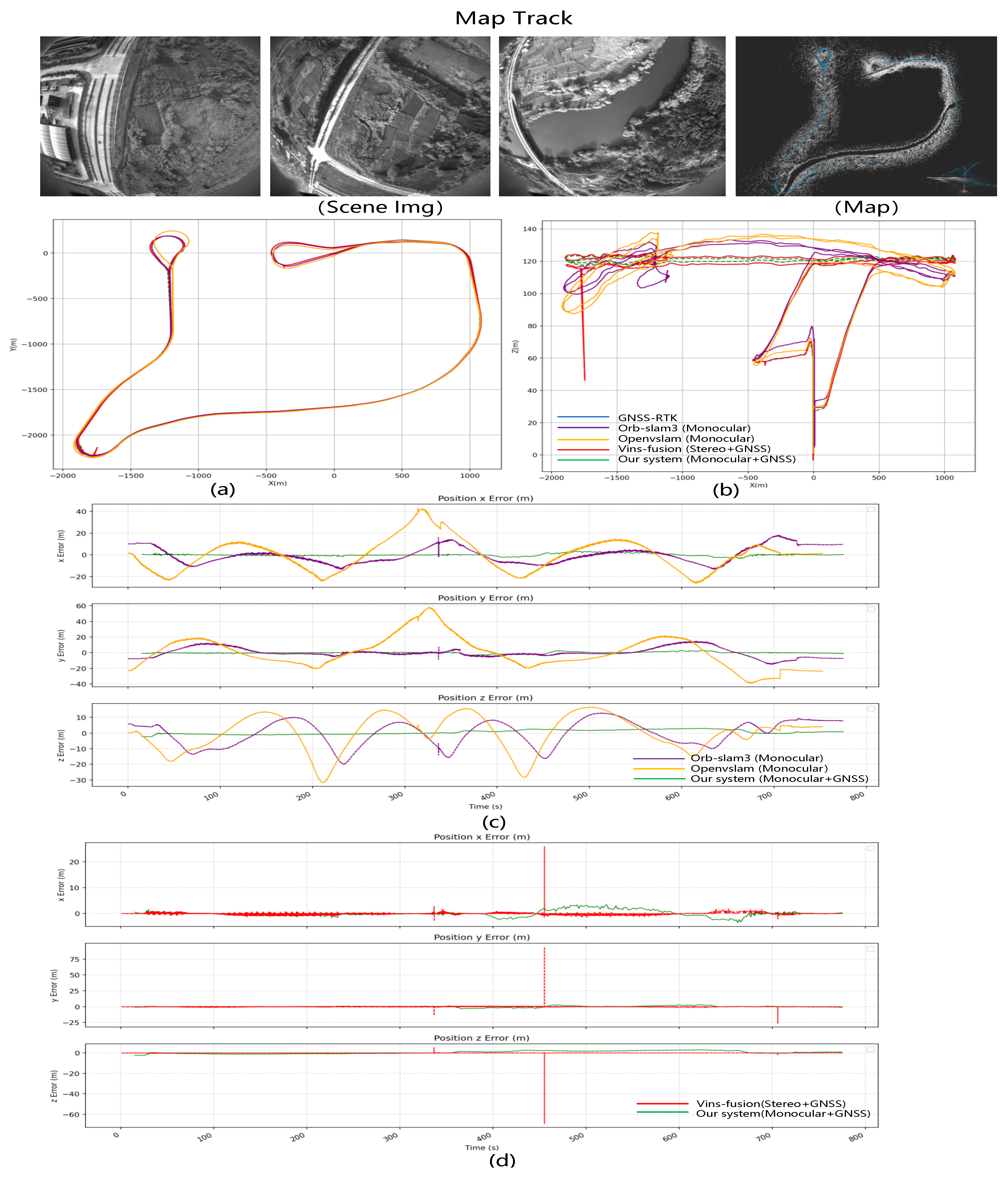
(2) Real-scene Data FlyReal-Data2 Comparative Experiment

Mapping data FlyReal-Data2: We use a drone to capture multiple sets of data in the normal environment. The trajectory of the drone is shown in Figure 14. The flight altitude is 120 m, the total mileage is 16.808 km, the frame rate of image acquisition is 15 frames, and the frame rate of GNSS acquisition is ten frames.

Compare Results: Compared with the other two sets of data, this set of data is not a trajectory of a large circular closed loop. This mode is more likely to cause cumulative errors and pose estimation errors, which is more challenging for pure visual SLAM systems and also highlights the importance of optimization with GNSS data. It can be seen from Figure 14c that Openvslam and ORB-SLAM3 monocular vision SLAM errors fluctuate more. The RSME of Openvslam and ORB-SLAM3 are 26.863 m and 12.416 m, respectively. Compared with the first set of test data, since the length of the whole track is 20 km shorter, their accumulated errors are also smaller. But compared with Vins-Fusion and our system, the error is still large. In this data group, the take-off and landing stages of the aircraft are relatively stable, so Vins-Fusion has no special prediction errors, and its RMSE is only 1.601 m. Our system performs well, and the RMSE is only 1.601 m, which is still the smallest among the four algorithms.

(3) Real-scene Data FlyReal-Data3 Comparative Experiment

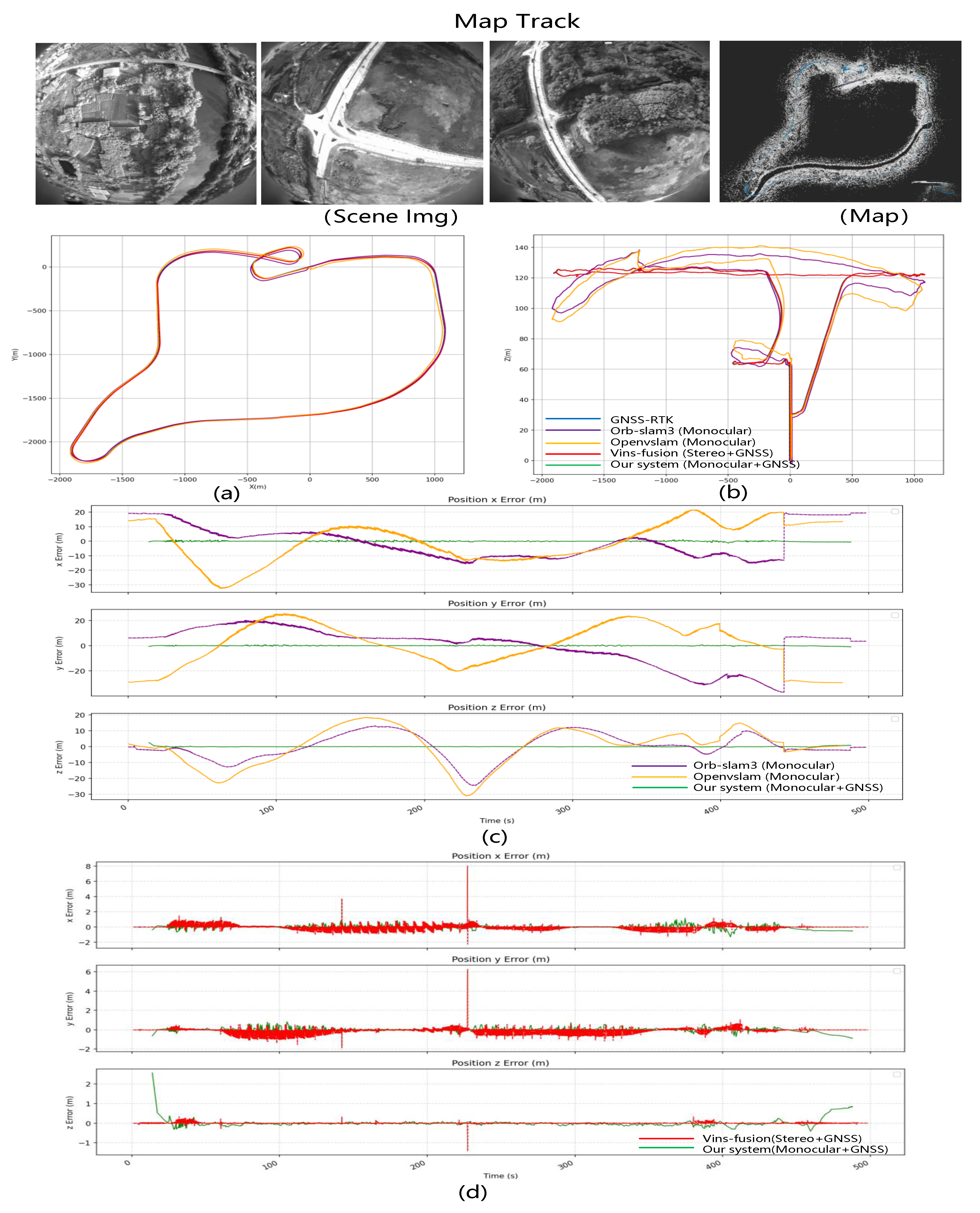
Mapping data FlyReal-Data3: We use a drone to capture multiple datasets in the normal environment. The trajectory of the drone is shown in Figure 15. The flight altitude is 120 m, the total mileage is 9.945 km, the image acquisition frame rate is 15 frames per second, and the frame rate of GNSS acquisition is 10 frames per second.

Compare Results: The length of the third set of data is 16.8 km, which is only half of the first set of data, and the shape is a closed great circle trajectory, which is beneficial further to reduce the cumulative error of the four algorithms. It can be seen from Figure 15b that the pose prediction error of Openvslam and ORB-SLAM at an altitude of 120 m is still huge. At the flight altitude of 60 m, the altitude prediction of the aircraft in the orbiting stage has an error of about 20 m. The RSMEs of Openvslam and ORB-SLAM3 are 24.196 m and 11.919 m, respectively. The flight trajectory of the aircraft is relatively smooth during the ascent and descent stages, so VINS-fusion also achieves good positioning results, and its RMSE is 0.501 m. The RMSE of our algorithm is 0.44 m, which is more accurate than Vins-Fusion and is the most accurate among the four algorithms.

The RSME of the data comparison of the four algorithms is shown in Table 2. Based on the comparison of several sets of data experiments, the pure visual monocular SLAM system represented by ORB-SLAM3 and Openvslam has a large error ratio in the case of long-distance aerial photography data, multiple altitude changes, and sudden rotation. Although these algorithms adopt loop closure detection and global optimization, the localization error is significant without the assistance of GNSS global absolute positioning information. In the experimental comparison of FlySImulation-Data1 and FlySImulation-Data3, our algorithm is more stable than Vins-Fusion, which also uses GNSS global optimization.

To enable experimental comparison, the experiment was conducted in an environment with reliable GNSS signals, resulting in VINS-Fusion achieving satisfactory positioning performance. However, real-world environments are highly complex and prone to sudden changes, with GNSS signals susceptible to malicious interference and disruption. Under the circumstance of extended GNSS unavailability, VINS-Fusion falls short of providing dependable positioning information for long-distance flight navigation missions due to the lack of global positioning support. Such a deficiency could entail significant hazards for small- to medium-sized logistics drones and large multirotor aircraft carrying passengers. Our proposed system overcomes GNSS constraints by utilizing high-precision pre-established visual maps to support global positioning. VINS-Fusion leverages corner point detection and optical flow tracking for its front-end implementation. When dealing with small-scale motion, the optical flow tracking method proves to be more advantageous than the feature point matching method. Our system utilizes ORB feature point matching for tracking the long-distance movement of UAVs in large scenes. This method is particularly advantageous regarding rotational invariance and contributes to the flexible flight tracking and positioning of UAVs in the air.

Despite ORB-SLAM3 and Openvslam’s ability to build offline maps for relocalization, their maps lack GNSS signal integration, resulting in considerable inaccuracies for long-distance navigation tasks.

E.

Computing Time

Table 3. The tracking thread and the mapping thread consume time.

Thread	Operation	Median (ms)	Mean (ms)	Std (ms)
TRACKING	Total	31.12	32.43	22.13
LOCAL MAPPING	KeyFrame Insertion	12.36	14.32	4.12
	Map Point Culling	0.032	2.4	0.95
	Map Point Creation	35.4	56.3	18.5
	Local BA	201.54	328.99	24.8
	Total	249.332	402.01	48.37

highlights the runtimes of the main operations performed in the tracking and mapping threads, demonstrating that our system can operate in real time at 20–30 frames per second. Since the tracking and mapping threads consistently operate on the active map, adding multi-mapping does not introduce significant overhead.

Table 4. The loop thread consumes time.

Loop	KeyFrame	Essential Graph Edges	Loop Detection (ms)	Essential Graph Optimization (s)	Total (s)
1	169	1761	32.52	1.378	33.898
2	732	8605	49.67	3.125	52.795
3	855	10740	53.54	4.133	57.673
4	1085	14781	64.65	6.632	71.282

summarizes the time consumed for loop closure. Running posture map optimization can keep the merging and cycle closing time below 0.5 s. Depending on the size of the associated keyframes on the map, performing a full beam adjustment during loop closure could potentially increase the timing by several seconds. In terms of map switching, the new map detection method only needs ten milliseconds to switch maps. In any case, since each operation is executed in a separate thread, the overall real-time performance of the system will not be affected.

All in all, our system can fully meet the needs of real-time navigation, and our processing speed is comparable to the latest ORB-SLAM3 system. While this is interesting, we do not further compare runtimes of other systems, as this would require a significant effort beyond the scope of this work.

Furthermore, we utilize the widely adopted SFM algorithm, Colmap, to construct offline three-dimensional sparse maps of these test datasets on a ground-based workstation. The time consumed for this process is presented in

Table 5. The time performance of popular SFM algorithms.

Datasets			Processing time(min)
Scene	Resolution	Number	Colmap				Ours
			Feature Extractor	Sequential Matching	Sparse Reconstruction	Total	Total
Scene1	1920 × 1080	388	0.134	0.696	12.89	13.729	0.274
Scene2	1920 × 1080	6721	2.751	5.212	>600	>600	2.491
Scene3	1920 × 1080	2541	1.039	3.668	616.13	620.837	2.456
Scene4	1920 × 1080	1129	0.443	3.212	185.67	189.325	0.991

.

It is evident that for datasets with a smaller number of images, such as Scene1, Colmap can produce a satisfactory sparse map in approximately 14 min. In contrast, our system only requires a total of 0.274 min. For datasets containing thousands of images, particularly video data, the process takes more than 10 h, and the results are also inconsistent in terms of quality. In contrast, our system only requires 2.491 min. In conclusion, when the dataset is small, and there is no strict requirement for processing time, SFM algorithms can be employed for denser three-dimensional map construction, leading to enhanced geographic localization accuracy. However, in cases of large datasets or emergency applications, the proposed algorithm simultaneously addresses both speed and accuracy concerns, enabling real-time geolocation.

In the context of our application scenarios, despite the higher speeds at which aerial robots operate, the associated optimization factors do not exhibit a substantial increase. In comparison to ground-based scenarios, the optimization elements involved are even fewer.

Firstly, our system employs a keyframe mechanism, meaning we do not store and optimize the pose of every image. Keyframes are generated, and their poses are recorded only when certain conditions are met. For example, a keyframe is triggered when the motion distance between adjacent frames surpasses a specific threshold. While aerial vehicles exhibit higher flight speeds, their elevated flying altitudes and downward-facing cameras provide a broader field of view. Compared to ground scenarios, aerial vehicles’ adjacent frames can observe larger overlapping scenes, requiring them to cover longer distances to trigger keyframe generation. Overall, this is manifested by a significantly lower number of keyframes generated from aerial viewpoints for the same area than ground viewpoints. Consequently, this greatly reduces the quantity of camera poses to be optimized as illustrated in Figure 16.

Compare the real-ground collected data, CarReal-Data1, with the real-flight collected data, FlyReal-Data1. The total trajectory length for ground operation in CarReal-Data1 is 4.986 km, with 3418 keyframes. The total aerial flight trajectory length for FlyReal-Data1 is 31.542 km, with 942 keyframes. By comparing these two sets of data, it becomes evident that the aerial flight perspective generates significantly fewer keyframes than the ground perspective.

Compare the simulated flight data, FlySimulation-Data1, with the real-flight collected data, FlyReal-Data1. The total aerial flight trajectory length for FlySimulation-Data1 is 58.9911 km, with 211 keyframes. FlySimulation-Data1 employs dense strip flight patterns in the air, resulting in longer distances but a more miniature overall scene. In contrast, FlyReal-Data1 consists of only three flight strips, yet it captures a larger scene area. The configuration of flight trajectories also affects the number of keyframes.

Compare the real-flight collected data, FlyReal-Data2, with the real-flight collected data, FlyReal-Data1. The total aerial flight trajectory length for FlyReal-Data2 is 9.94 km, with 681 keyframes. For the same scene, FlyReal-Data2 covered only one flight strip, whereas FlyReal-Data1 covered three. Despite this difference, the increase in keyframes is only around 160 frames, accounting for an approximate 23% increase.

Furthermore, for local optimization during backend bundle adjustment (BA) computations, controlling the scale of the graph optimization becomes necessary. Hence, the adoption of a sliding window strategy is employed. This strategy involves consistently fixing a set of N frames. The result is that BA optimization is constrained within a temporal window. Once new image frames are introduced, old image frames are discarded. This approach significantly reduces the computational scale compared to traditional bundle adjustment.

Lastly, for global optimization, the nonlinear optimization library G2O is employed. The optimization process is carried out in a dedicated thread to enhance runtime efficiency. We utilize NUC microcomputers equipped with an Intel i7 processor featuring four cores and eight threads in its processing configuration. Our system can achieve real-time online optimization based on the current scene scale. In addition to online real-time mapping and optimization, we can also establish maps during the offline stage. During the localization phase, the map can be loaded for positioning, further alleviating the computational burden on the onboard processing unit.

In summary, aerial robots offer an enhanced vertical and expansive field of view. As the flight altitude increases for the same area, the generated number of keyframes is fewer compared to ground viewpoints. As a result, a reduced number of keyframe poses require optimization, leading to improved speed in graph optimization. When integrated with the optimization strategies employed across the entire system, this approach effectively fulfills the speed requisites of aerial drones.

7. Conclusions

We have presented a novel LD-SLAM with monocular, pin-hole, and fisheye cameras for long-distance visual localization and mapping. The main innovations of this paper are as follows: we propose a novel GNSS and visual information fusion method for offline mapping, which can successfully reduce cumulative error and enable high-precision long-distance mapping with a monocular camera. We also propose a multimap approach. Accuracy and robustness in complex scenes can be further improved by automatic segmentation, merging, and switching methods. Based on the abovementioned techniques, we develop a novel, complete, high-performance visual navigation and positioning system using only one camera. In scenarios of complete GNSS loss during the execution of transportation tasks by UAVs and eVTOL aircraft, multiple maps are utilized as a substitute for GNSS to maintain global positioning information. Our experimental results show that LD-SLAM can effectively use multimap visual navigation and achieve levels of accuracy that exceed existing systems over tens of kilometers. The system offers advantages in construction cost, complexity reduction, and ease of integration, enabling continuous, robust, and precise localization in large-scale and complex environments. Currently, low-texture environments are the most common cause of LD-SLAM failures. In this work, we automatically generate multimaps to avoid these low-texture regions, enhancing the overall system’s robustness over long distances. In the future, an interesting work could be to use the latest advances in CNN capabilities for promising local feature extraction and adaptation. Another interesting research direction could be to develop multiple sensing techniques to extract appropriate features. LD-SLAM employs an optimization algorithm applied to the factor graph, which is particularly suitable for multi-sensor fusion. In the future, it can easily integrate measurements from other sensors as new factors into the framework. We are exploring the above two ideas for more robust map generation in challenging, long-distance scenes encompassing low-texture regions.

References

1. Buehler, M.; Iagnemma, K.; Singh, S. The DARPA Urban Challenge: Autonomous Vehicles in City Traffic; Springer: Berlin/Heidelberg, Germany, 2009; Volume 56. [Google Scholar]
2. Wan, G.; Yang, X.; Cai, R.; Li, H.; Zhou, Y.; Wang, H.; Song, S. Robust and precise vehicle localization based on multi-sensor fusion in diverse city scenes. In Proceedings of the 2018 IEEE International Conference on robotics and Automation (ICRA), Brisbane, QLD, Australia, 21–25 May 2018; IEEE: New York, NY, USA, 2018; pp. 4670–4677. [Google Scholar]
3. Meng, X.; Wang, H.; Liu, B. A robust vehicle localization approach based on gnss/imu/dmi/lidar sensor fusion for autonomous vehicles. Sensors 2017, 17, 2140. [Google Scholar] [CrossRef] [PubMed]
4. Cadena, C.; Carlone, L.; Carrillo, H.; Latif, Y.; Scaramuzza, D.; Neira, J.; Reid, I.; Leonard, J.J. Past, present, and future of simultaneous localization and mapping: Toward the robust-perception age. IEEE Trans. Robot. 2016, 32, 1309–1332. [Google Scholar] [CrossRef]
5. Mur-Artal, R.; Montiel, J.M.M.; Tardos, J.D. ORB-SLAM: A versatile and accurate monocular SLAM system. IEEE Trans. Robot. 2015, 31, 1147–1163. [Google Scholar] [CrossRef]
6. Mur-Artal, R.; Tardós, J.D. Orb-slam2: An open-source slam system for monocular, stereo, and rgb-d cameras. IEEE Trans. Robot. 2017, 33, 1255–1262. [Google Scholar] [CrossRef]
7. Engel, J.; Koltun, V.; Cremers, D. Direct sparse odometry. IEEE Trans. Pattern Anal. Mach. Intell. 2017, 40, 611–625. [Google Scholar] [CrossRef]
8. Qin, T.; Li, P.; Shen, S. Vins-mono: A robust and versatile monocular visual-inertial state estimator. IEEE Trans. Robot. 2018, 34, 1004–1020. [Google Scholar] [CrossRef]
9. Campos, C.; Elvira, R.; Rodríguez, J.J.G.; Montiel, J.M.; Tardós, J.D. Orb-slam3: An accurate open-source library for visual, visual-inertial, and multimap slam. IEEE Trans. Robot. 2021, 37, 1874–1890. [Google Scholar] [CrossRef]
10. Qin, T.; Li, P.; Shen, S. Relocalization, global optimization and map merging for monocular visual-inertial SLAM. In Proceedings of the 2018 IEEE International Conference on Robotics and Automation (ICRA), Brisbane, QLD, Australia, 21–25 May 2018; IEEE: New York, NY, USA, 2018; pp. 1197–1204. [Google Scholar]
11. Qin, T.; Cao, S.; Pan, J.; Shen, S. A general optimization-based framework for global pose estimation with multiple sensors. arXiv Prepr. 2019, arXiv:1901.03642. [Google Scholar]
12. Cao, S.; Lu, X.; Shen, S. GVINS: Tightly coupled GNSS-visual-inertial fusion for smooth and consistent state estimation. IEEE Trans. Robot. 2022, 38, 2004–2021. [Google Scholar] [CrossRef]
13. Niu, X.; Tang, H.; Zhang, T.; Fan, J.; Liu, J. IC-GVINS: A Robust, Real-Time, INS-Centric GNSS-Visual-Inertial Navigation System. IEEE Robot. Autom. Lett. 2022, 8, 216–223. [Google Scholar] [CrossRef]
14. Xiong, L.; Kang, R.; Zhao, J.; Zhang, P.; Xu, M.; Ju, R.; Ye, C.; Feng, T. G-VIDO: A vehicle dynamics and intermittent GNSS-aided visual-inertial state estimator for autonomous driving. IEEE Trans. Intell. Transp. Syst. 2021, 23, 11845–11861. [Google Scholar] [CrossRef]
15. Aldibaja, M.; Suganuma, N.; Yoneda, K.; Yanase, R. Challenging Environments for Precise Mapping Using GNSS/INS-RTK Systems: Reasons and Analysis. Remote Sens. 2022, 14, 4058. [Google Scholar] [CrossRef]
16. Davison, A.J.; Reid, I.D.; Molton, N.D.; Stasse, O. MonoSLAM: Real-time single camera SLAM. IEEE Trans. Pattern Anal. Mach. Intell. 2007, 29, 1052–1067. [Google Scholar] [CrossRef]
17. Klein, G.; Murray, D. Parallel tracking and mapping for small AR workspaces. In Proceedings of the 2007 6th IEEE and ACM International Symposium on Mixed and Augmented Reality, Nara, Japan, 13–16 November 2007; IEEE: New York, NY, USA, 2007; pp. 225–234. [Google Scholar]
18. Strasdat, H.; Montiel, J.; Davison, A.J. Scale drift-aware large scale monocular SLAM. Robot. Sci. Syst. VI 2010, 2, 7. [Google Scholar]
19. Strasdat, H.; Davison, A.J.; Montiel, J.M.; Konolige, K. Double window optimisation for constant time visual SLAM. In Proceedings of the 2011 International Conference on Computer Vision, Barcelona, Spain, 6–13 November 2011; IEEE: New York, NY, USA, 2011; pp. 2352–2359. [Google Scholar]
20. Gálvez-López, D.; Tardos, J.D. Bags of binary words for fast place recognition in image sequences. IEEE Trans. Robot. 2012, 28, 1188–1197. [Google Scholar] [CrossRef]
21. Fu, Q.; Yu, H.; Wang, X.; Yang, Z.; Zhang, H.; Mian, A. FastORB-SLAM: A fast ORB-SLAM method with Coarse-to-Fine descriptor independent keypoint matching. arXiv Prepr. 2020, arXiv:2008.09870. [Google Scholar]
22. Sumikura, S.; Shibuya, M.; Sakurada, K. OpenVSLAM: A versatile visual SLAM framework. In Proceedings of the 27th ACM International Conference on Multimedia, 21–25 October 2019; pp. 2292–2295. [Google Scholar]
23. Engel, J.; Schöps, T.; Cremers, D. LSD-SLAM: Large-scale direct monocular SLAM. In Proceedings of the Computer Vision–ECCV 2014: 13th European Conference, Zurich, Switzerland, 6–12 September 2014; Proceedings, Part II 13. Springer: Berlin/Heidelberg, Germany, 2014; pp. 834–849. [Google Scholar]
24. Forster, C.; Pizzoli, M.; Scaramuzza, D. SVO: Fast semi-direct monocular visual odometry. In Proceedings of the 2014 IEEE International Conference on Robotics and Automation (ICRA), Hong Kong, China, 31 May–7 June 2014; IEEE: New York, NY, USA, 2014; pp. 15–22. [Google Scholar]
25. Forster, C.; Zhang, Z.; Gassner, M.; Werlberger, M.; Scaramuzza, D. SVO: Semidirect visual odometry for monocular and multicamera systems. IEEE Trans. Robot. 2016, 33, 249–265. [Google Scholar] [CrossRef]
26. Wang, R.; Schworer, M.; Cremers, D. Stereo DSO: Large-scale direct sparse visual odometry with stereo cameras. In Proceedings of the IEEE International Conference on Computer Vision, Venice, Italy, 22–29 October 2017; pp. 3903–3911. [Google Scholar]
27. Gao, X.; Wang, R.; Demmel, N.; Cremers, D. LDSO: Direct sparse odometry with loop closure. In Proceedings of the 2018 IEEE/RSJ International Conference on Intelligent Robots and Systems (IROS), Madrid, Spain, 1–5 October 2018; IEEE: New York, NY, USA, 2018; pp. 2198–2204. [Google Scholar]
28. Lee, S.H.; Civera, J. Loosely-coupled semi-direct monocular slam. IEEE Robot. Autom. Lett. 2018, 4, 399–406. [Google Scholar] [CrossRef]
29. Von Stumberg, L.; Usenko, V.; Cremers, D. Direct sparse visual-inertial odometry using dynamic marginalization. In Proceedings of the 2018 IEEE International Conference on Robotics and Automation (ICRA), Brisbane, QLD, Australia, 21–25 May 2018; IEEE: New York, NY, USA, 2018; pp. 2510–2517. [Google Scholar]
30. Adorno, B.; Aghajani Pedram, S.; Agrawal, S.; Aguinaga, I.; Alambeigi, F.; Albert, K.; Alenya, G.; Allevi, F.; Aloi, V.; Alonso, I.; et al. 2020 Index IEEE Transactions on Robotics Vol. 36. IEEE Trans. Robot. 2020, 36, 1819–1840. [Google Scholar]
31. Shahoud, A.; Shashev, D.; Shidlovskiy, S. Visual navigation and path tracking using street geometry information for image alignment and serving. Drones 2022, 6, 107. [Google Scholar] [CrossRef]
32. Mourikis, A.I.; Roumeliotis, S.I. A multi-state constraint Kalman filter for vision-aided inertial navigation. In Proceedings of the 2007 IEEE International Conference on Robotics and Automation, Rome, Italy, 10–14 April 2007; IEEE: New York, NY, USA, 2007; pp. 3565–3572. [Google Scholar]
33. Leutenegger, S.; Furgale, P.; Rabaud, V.; Chli, M.; Konolige, K.; Siegwart, R. Keyframe-based visual-inertial slam using nonlinear optimization. In Proceedings of the Robotis Science and Systems (RSS), Berlin, Germany, 24–28 June 2013; pp. 1–8. [Google Scholar]
34. Leutenegger, S.; Lynen, S.; Bosse, M.; Siegwart, R.; Furgale, P. Keyframe-based visual–inertial odometry using nonlinear optimization. Int. J. Robot. Res. 2015, 34, 314–334. [Google Scholar] [CrossRef]
35. Mur-Artal, R.; Tardós, J.D. Visual-inertial monocular SLAM with map reuse. IEEE Robot. Autom. Lett. 2017, 2, 796–803. [Google Scholar] [CrossRef]
36. Lupton, T.; Sukkarieh, S. Visual-inertial-aided navigation for high-dynamic motion in built environments without initial conditions. IEEE Trans. Robot. 2011, 28, 61–76. [Google Scholar] [CrossRef]
37. Forster, C.; Carlone, L.; Dellaert, F.; Scaramuzza, D. On-manifold preintegration for real-time visual-inertial odometry. IEEE Trans. Robot. 2016, 33, 1–21. [Google Scholar] [CrossRef]
38. Usenko, V.; Demmel, N.; Schubert, D.; Stückler, J.; Cremers, D. Visual-inertial mapping with non-linear factor recovery. IEEE Robot. Autom. Lett. 2019, 5, 422–429. [Google Scholar] [CrossRef]
39. Rosinol, A.; Abate, M.; Chang, Y.; Carlone, L. Kimera: An open-source library for real-time metric-semantic localization and mapping. In Proceedings of the 2020 IEEE International Conference on Robotics and Automation (ICRA), Paris, France, 31 May–31 August 2020; IEEE: New York, NY, USA, 2020; pp. 1689–1696. [Google Scholar]
40. Zhang, Y.; Huang, F. Panoramic visual SLAM technology for spherical images. Sensors 2021, 21, 705. [Google Scholar] [CrossRef]
41. Fu, Q.; Wang, J.; Yu, H.; Ali, I.; Guo, F.; He, Y.; Zhang, H. Pl-vins: Real-time monocular visual-inertial slam with point and line features. arXiv Prepr. 2020, arXiv:2009.07462. [Google Scholar]
42. Gu, N.; Xing, F.; You, Z. Visual/Inertial/GNSS Integrated Navigation System under GNSS Spoofing Attack. Remote Sens. 2022, 14, 5975. [Google Scholar] [CrossRef]
43. Vidal, A.R.; Rebecq, H.; Horstschaefer, T.; Scaramuzza, D. Ultimate SLAM? Combining events, images, and IMU for robust visual SLAM in HDR and high-speed scenarios. IEEE Robot. Autom. Lett. 2018, 3, 994–1001. [Google Scholar] [CrossRef]
44. Groves, P.D. NAVIGATION SYSTEMS. In Principes of GNSS, Inertial and Multisensor Integrated; Artech: Singapore, 2008; pp. 1–17. [Google Scholar]
45. Jin, R.; Liu, J.; Zhang, H.; Niu, X. Fast and accurate initialization for monocular vision/INS/GNSS integrated system on land vehicle. IEEE Sens. J. 2021, 21, 26074–26085. [Google Scholar] [CrossRef]
46. Zhang, Q.; Li, S.; Xu, Z.; Niu, X. Velocity-based optimization-based alignment (VBOBA) of low-end MEMS IMU/GNSS for low dynamic applications. IEEE Sens. J. 2020, 20, 5527–5539. [Google Scholar] [CrossRef]
47. Eade, E.; Drummond, T. Unified loop closing and recovery for real time monocular SLAM. In Proceedings of the British Machine Vision Conference, Leeds, UK, 18 August 2008; Volume 13, p. 136. [Google Scholar]
48. Castle, R.; Klein, G.; Murray, D.W. Video-rate localization in multiple maps for wearable augmented reality. In Proceedings of the 2008 12th IEEE International Symposium on Wearable Computers, Pittsburgh, PA, USA, 28 September–1 October 2008; IEEE: New York, NY, USA, 2008; pp. 15–22. [Google Scholar]
49. Forster, C.; Lynen, S.; Kneip, L.; Scaramuzza, D. Collaborative monocular slam with multiple micro aerial vehicles. In Proceedings of the 2013 IEEE/RSJ International Conference on Intelligent Robots and Systems, Tokyo, Japan, 3–7 November 2013; IEEE: New York, NY, USA, 2013; pp. 3962–3970. [Google Scholar]
50. Riazuelo, L.; Civera, J.; Montiel, J.M. C2tam: A cloud framework for cooperative tracking and mapping. Robot. Auton. Syst. 2014, 62, 401–413. [Google Scholar] [CrossRef]
51. Morrison, J.G.; Gálvez-López, D.; Sibley, G. MOARSLAM: Multiple operator augmented RSLAM. In Proceedings of the Distributed Autonomous Robotic Systems: The 12th International Symposium, London, UK, 6–9 November 2016; Springer: Berlin/Heidelberg, Germany, 2016; pp. 119–132. [Google Scholar]
52. Schmuck, P.; Chli, M. Multi-uav collaborative monocular slam. In Proceedings of the 2017 IEEE International Conference on Robotics and Automation (ICRA), Singapore, 29 May–3 June 2017; IEEE: New York, NY, USA, 2017; pp. 3863–3870. [Google Scholar]
53. Schmuck, P.; Chli, M. CCM-SLAM: Robust and efficient centralized collaborative monocular simultaneous localization and mapping for robotic teams. J. Field Robot. 2019, 36, 763–781. [Google Scholar] [CrossRef]
54. Daoud, H.A.; Md. Sabri, A.Q.; Loo, C.K.; Mansoor, A.M. SLAMM: Visual monocular SLAM with continuous mapping using multiple maps. PLoS ONE 2018, 13, e0195878. [Google Scholar] [CrossRef] [PubMed]
55. Liu, Y.; Miura, J. RDS-SLAM: Real-time dynamic SLAM using semantic segmentation methods. IEEE Access 2021, 9, 23772–23785. [Google Scholar] [CrossRef]
56. Ming, D.; Wu, X. Research on Monocular Vision SLAM Algorithm for Multi-map Fusion and Loop Detection. In Proceedings of the 2022 6th International Conference on Automation, Control and Robots (ICACR), Shanghai, China, 23–25 September 2022; IEEE: New York, NY, USA, 2022; pp. 212–216. [Google Scholar]
57. Liu, B.; Zhang, Z.; Hao, D.; Liu, G.; Lu, H.; Meng, Y.; Lu, X. Collaborative Visual Inertial SLAM with KNN Map Matching. In Proceedings of the 2022 12th International Conference on CYBER Technology in Automation, Control, and Intelligent Systems (CYBER), Baishan, China, 27–31 July 2022; IEEE: New York, NY, USA, 2022; pp. 1177–1181. [Google Scholar]
58. Seçkin, A.Ç.; Karpuz, C.; Özek, A. Feature matching based positioning algorithm for swarm robotics. Comput. Electr. Eng. 2018, 67, 807–818. [Google Scholar] [CrossRef]
59. Grisetti, G.; Kümmerle, R.; Strasdat, H.; Konolige, K. g2o: A general framework for (hyper) graph optimization. In Proceedings of the IEEE International Conference on Robotics and Automation (ICRA), Shanghai, China, 9–13 May 2011; pp. 9–13. [Google Scholar]
Figure 1. The system framework illustrates the processes taken by the tracking, local mapping, and loop-closing threads. The map and main components of the place recognition module are included in the illustration.
Remotesensing 15 04442 g001
Figure 2. GNSS-assisted optimization algorithm framework based on dynamic range.
Remotesensing 15 04442 g002
Figure 3. Multi-map-matching fusion process based on GNSS vision.
Remotesensing 15 04442 g003
Figure 4. The drone and ground experimental platform we constructed. The camera and minicomputer can be mounted on drones and ground vehicles.
Remotesensing 15 04442 g004
Figure 5. Experimental dataset. The experimental dataset is divided into test data collected by aerial drones and test data collected by ground vehicles. The UAV test dataset is further divided into a simulation dataset and a real dataset.
Remotesensing 15 04442 g005
Figure 6. Mapping results of simulation scene drone aerial photography data FlySImulation-Data1. Comparison of mapping in two modes: pure vision SLAM and vision + GNSS optimization. (a) The mapping data, (b) the comparison of 3D trajectory of the mapping results in XYZ space, (c) the comparison of 2D trajectory in XY plane, (d) the comparison of 2D trajectory in XZ plane, and (e) the error comparison between the visual SLAM mapping results and the visual+GNSS optimized mapping results over time.
Remotesensing 15 04442 g006
Figure 7. Localization results of simulation aerial photography data FlySimulation-Data2. Comparison of localization in two modes: pure vision SLAM and vision + GNSS optimization. (a) The ground truth flight trajectory, (b) the comparison of the 3D trajectory of the localization results in XYZ space, (c) the comparison of 2D trajectory in XY plane, (d) the comparison of 2D trajectory in XZ plane, and (e) the error comparison between the visual SLAM mapping results and the visual+GNSS optimized mapping results over time.
Remotesensing 15 04442 g007
Figure 8. Mapping results of real scene drone aerial photography data FlyReal-Data1. Comparison of mapping in two modes: pure vision SLAM and vision + GNSS optimization. (a) The mapping data, (b) the comparison of 3D trajectory of the mapping results in XYZ space, (c) the comparison of 2D trajectory in XY plane, (d) the comparison of 2D trajectory in XZ plane, and (e) the error comparison between the visual SLAM mapping results and the visual+GNSS optimized mapping results over time.
Remotesensing 15 04442 g008
Figure 9. Localization results of real aerial photography data FlyReal-Data2. Comparison of localization in two modes: pure vision SLAM and vision + GNSS optimization. (a) The ground truth flight trajectory, (b) the comparison of 3D trajectory of the localization results in XYZ space, (c) the comparison of 2D trajectory in XY plane, (d) the comparison of 3D trajectory in XZ plane, and (e) the error comparison between the visual SLAM mapping results and the visual+GNSS optimized mapping results over time.
Remotesensing 15 04442 g009
Figure 10. Localization results of real aerial photography data FlyReal-Data3. Comparison of localization in two modes: pure vision SLAM and vision + GNSS optimization. (a) The ground truth flight trajectory, (b) the comparison of 3D trajectory of the localization results in XYZ space, (c) the comparison of 2D trajectory in XY plane, (d) the comparison of 2D trajectory in XZ plane, and (e) the error comparison between the visual SLAM mapping results and the visual+GNSS optimized mapping results over time.
Remotesensing 15 04442 g010
Figure 11. Mapping results of ground vehicle data in real urban environment CarReal-Data1. Comparison of mapping in two modes: pure vision SLAM and vision + GNSS optimization. (a) The mapping data, (b) the comparison of 3D trajectory of the mapping results in XYZ space, (c) the comparison of 2D trajectory in XY plane, (d) the comparison of 2D trajectory in XZ plane, and (e) the error comparison between the visual SLAM mapping results and the visual + GNSS optimized mapping results over time.
Remotesensing 15 04442 g011
Figure 12. Localizationresults of ground vehicle data CarReal-Data2 in real urban environment. Comparison of localization in two modes: pure vision SLAM and vision + GNSS optimization. (a) the ground truth flight trajectory, (b) the comparison of the 3D trajectory of the localization results in XYZ space, (c) the comparison of 2D trajectory in XY plane, (d) the comparison of 2D trajectory in XZ plane, and (e) the error comparison between the visual SLAM mapping results and the visual + GNSS optimized mapping results over time.
Remotesensing 15 04442 g012
Figure 13. Relative pose errors versus evaluated distances for ORB-SLAM3, Openvslam, VINS-Fusion, and our system in the airborne dataset FlyReal-Data1. (a) The comparison of 2D trajectory in the XZ plane, (b) the comparison of 2D trajectory in the XZ plane, (c) the comparison of the trajectory error in XYZ direction with the algorithm using pure visual localization, and (d) comparison with the vision and GNSS information fusion algorithm for localization in the XYZ direction trajectory error.
Remotesensing 15 04442 g013
Figure 14. Relative pose errors versus evaluated distances for ORB-SLAM3, Openvslam, VINS-Fusion, and our system in the airborne dataset FlyReal-Data2. (a) The comparison of 2D trajectory in the XZ plane, (b) the comparison of 2D trajectory in the XZ plane, (c) the comparison of the trajectory error in XYZ direction with the algorithm using pure visual localization, and (d) comparison with the vision and GNSS information fusion algorithm for the XYZ direction trajectory error localization.
Remotesensing 15 04442 g014
Figure 15. Relative pose errors versus evaluated distances for ORB-SLAM3, Openvslam, VINS-Fusion, and our system in the airborne dataset FlyReal-Data3. (a) The comparison of 2D trajectory in the XZ plane, (b) the comparison of 2D trajectory in the XZ plane, (c) the comparison of the trajectory error in XYZ direction with the algorithm using pure visual localization, and (d) comparison with the vision and GNSS information fusion algorithm for localization in the XYZ direction trajectory error.
Remotesensing 15 04442 g015
Figure 16. Both the scene, collection angles, and overlap will influence the number of keyframes to be optimized.
Remotesensing 15 04442 g016