
The Influence of Visual Landscapes on Road Traffic Safety: An Assessment Using Remote Sensing and Deep Learning

 ,
,  , , and
Abstract
1. Introduction
2. Data and Methods
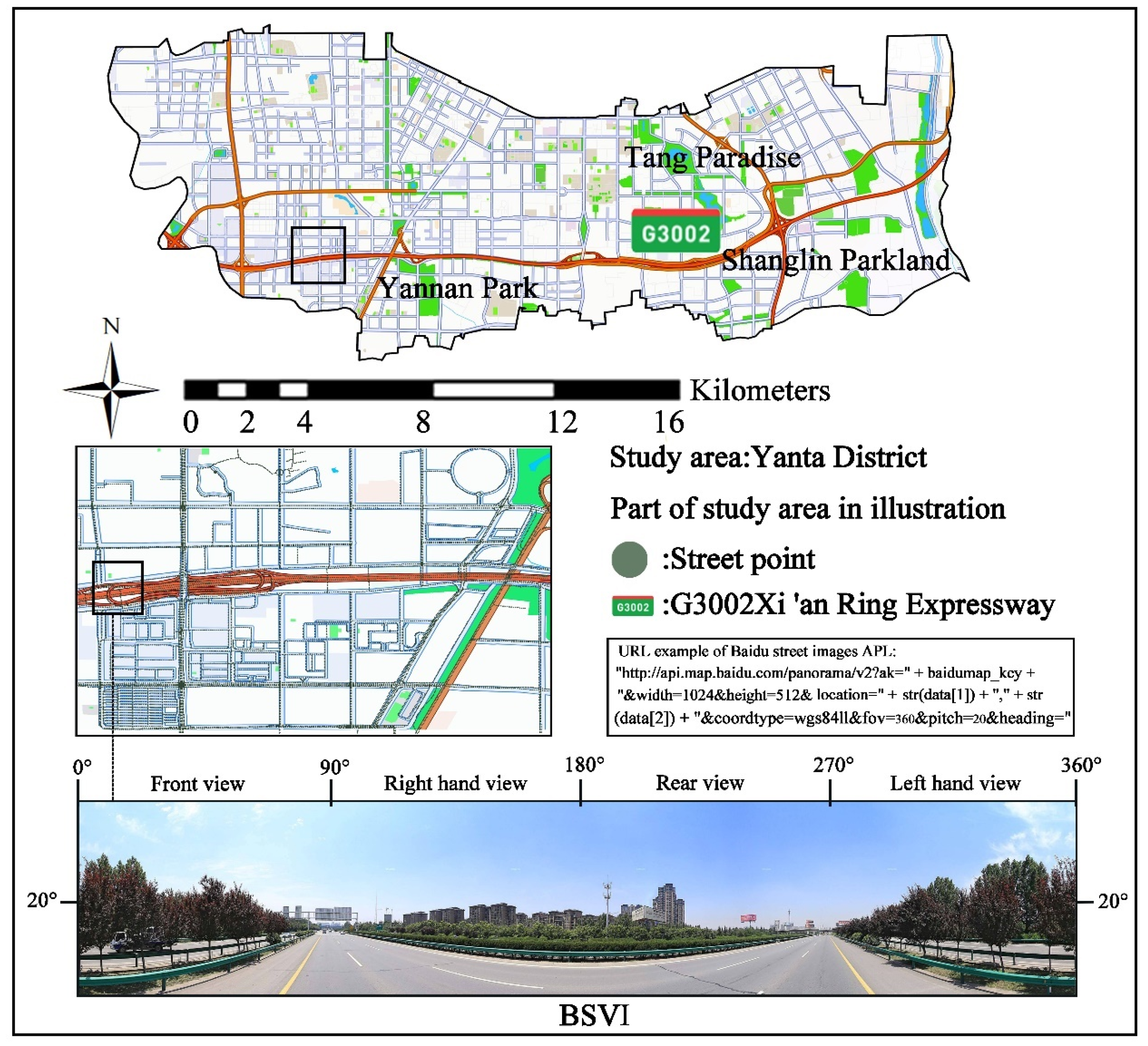
2.1. Study Area
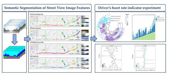
2.2. Research Framework
2.3. BSVI Data Collection
2.4. Extraction of Drivers’ Visual Environment Elements from BSVIs
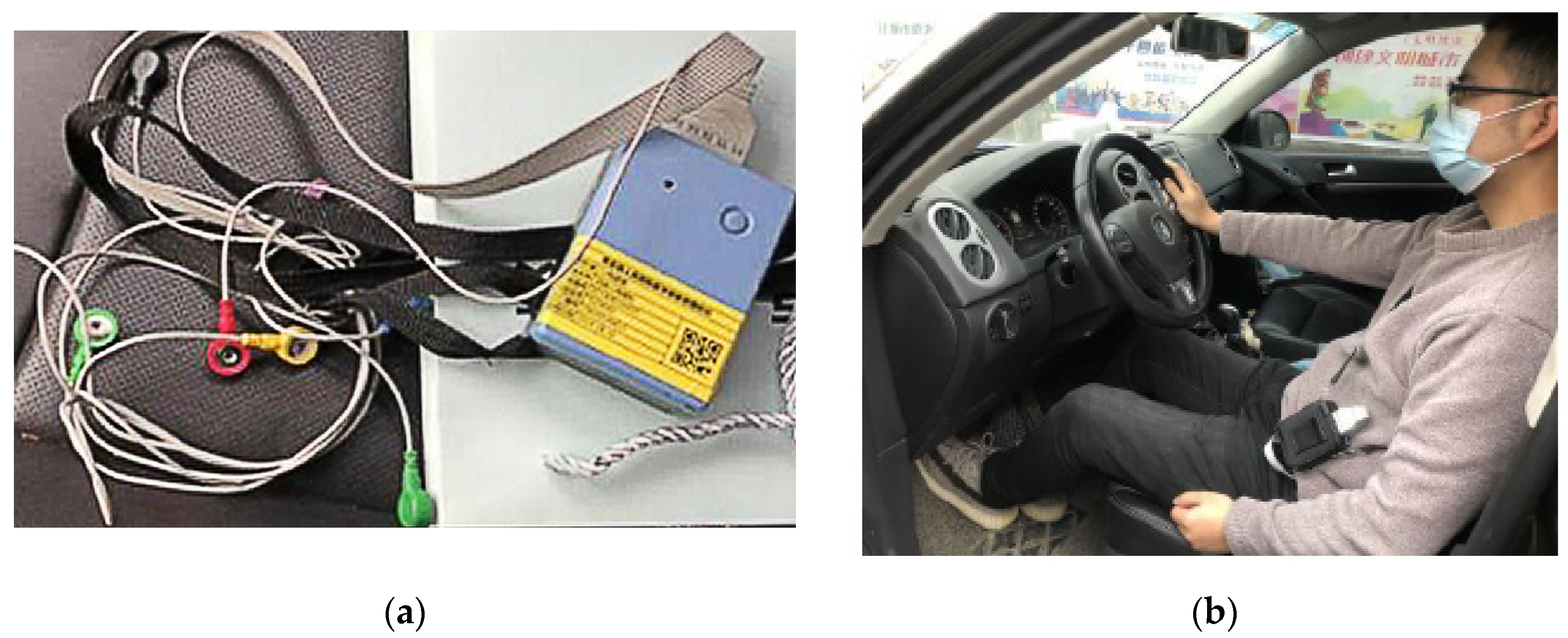
2.5. Driver Heart Rate Indicator Experiment
2.5.1. Data Collection from Field Experiments
2.5.2. Construction of a Relationship Model for the Effect of Highway Visual Landscape Complexity on Heart Rate Considering Driving Speed
3. Results
3.1. Spatial Distribution Characteristics of Urban Street Visual Landscape Elements
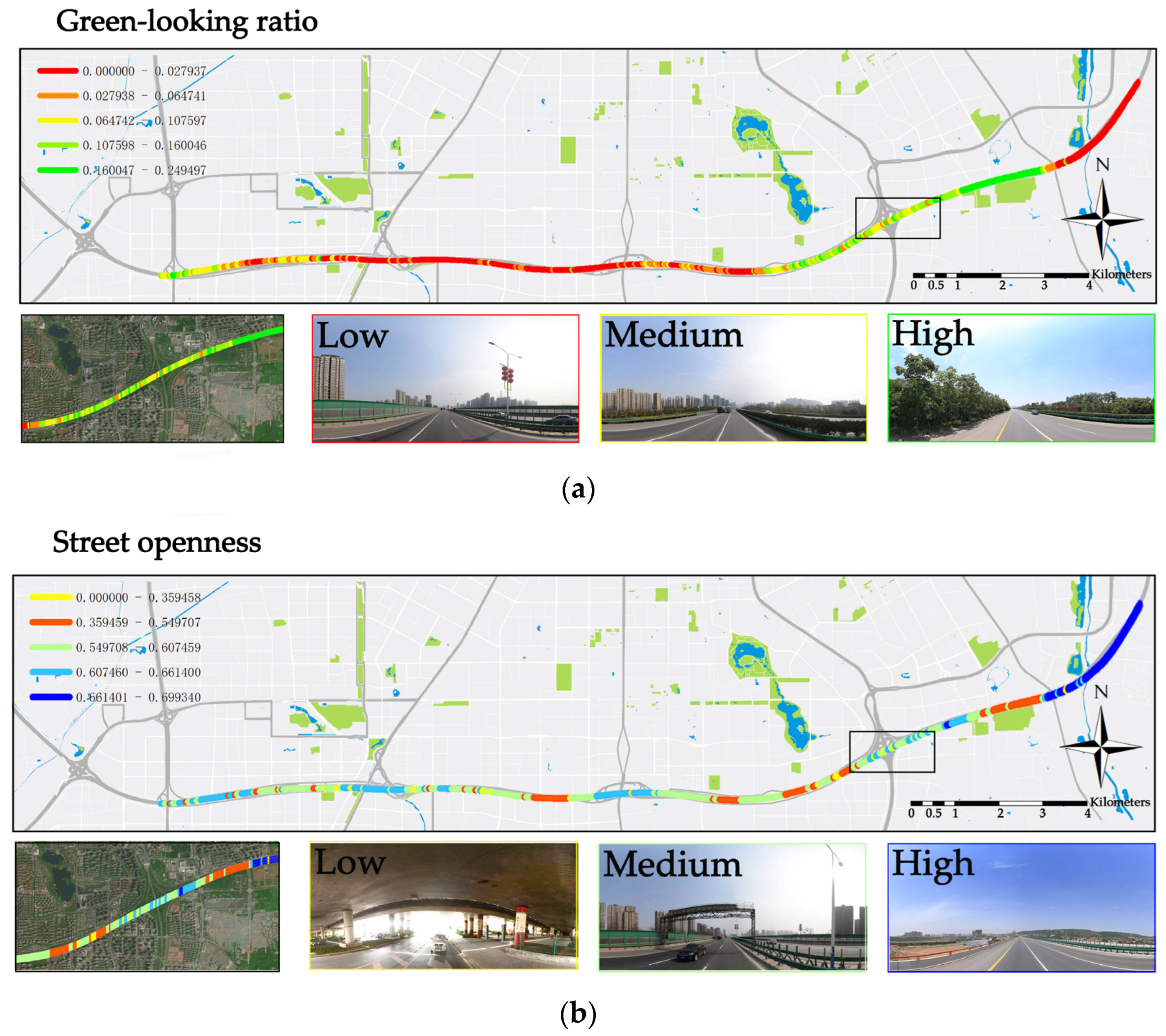
3.1.1. Spatial Distribution of Different Visual Landscape Elements
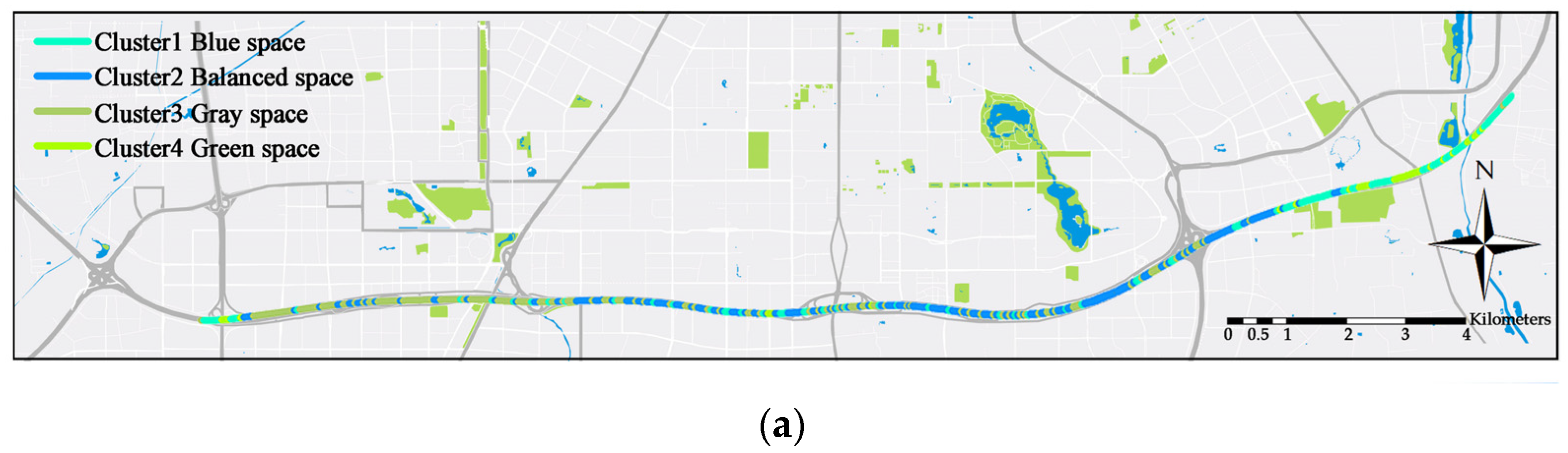
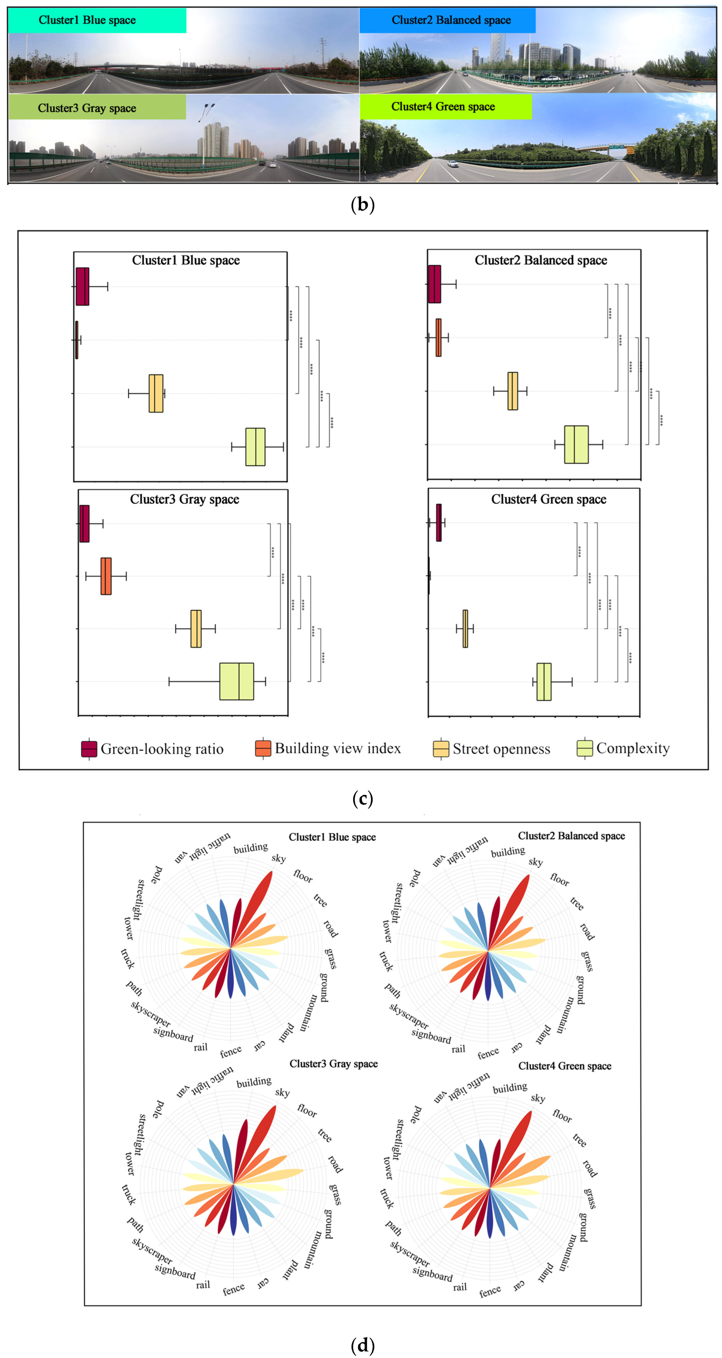
3.1.2. Cluster Analysis and Spatial Distribution of Visual Landscape Elements
3.2. Impact of Visual Landscape on Driving Fatigue
3.2.1. Model Fitting and Model Validation
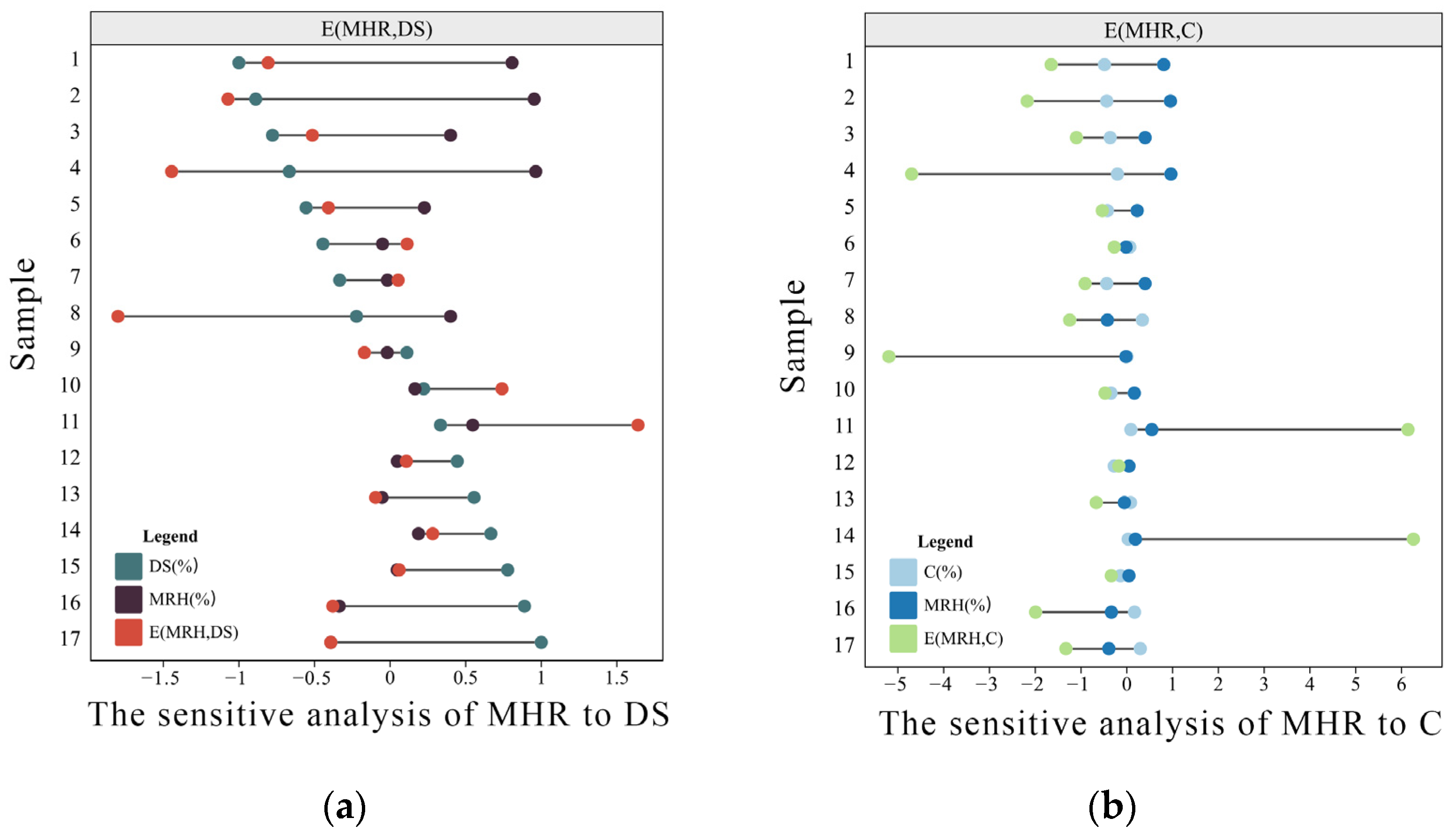
3.2.2. Sensitivity Analysis
4. Discussion
5. Conclusions
Author Contributions
Funding
Data Availability Statement
Acknowledgments
Conflicts of Interest
References
- Guo, B.; Wu, H.; Pei, L.; Zhu, X.; Zhang, D.; Wang, Y.; Luo, P. Study on the spatiotemporal dynamic of ground-level ozone concentrations on multiple scales across China during the blue sky protection campaign. Environ. Int. 2022, 170, 107606. [Google Scholar] [CrossRef] [PubMed]
- Wang, X.; Luo, P.; Zheng, Y.; Duan, W.; Wang, S.; Zhu, W.; Zhang, Y.; Nover, D. Drought Disasters in China from 1991 to 2018: Analysis of Spatiotemporal Trends and Characteristics. Remote Sens. 2023, 15, 1708. [Google Scholar] [CrossRef]
- Naik, B.; Tung, L.-W.; Zhao, S.; Khattak, A.J. Weather impacts on single-vehicle truck crash injury severity. J. Saf. Res. 2016, 58, 57–65. [Google Scholar] [CrossRef] [PubMed]
- Zhao, S.; Khattak, A.J. Injury severity in crashes reported in proximity of rail crossings: The role of driver inattention. J. Transp. Saf. Secur. 2018, 10, 507–524. [Google Scholar] [CrossRef]
- Yijun, X.; Junfeng, G.; Yong, Y.; Xiaolin, Y.; Wentao, H. Classifying Driving Fatigue Based on Combined Entropy Measure Using EEG Signals. Int. J. Control Autom. 2016, 9, 329–338. [Google Scholar]
- Parsons, R.; Tassinary, L.G.; Ulrich, R.S.; Hebl, M.R.; Grossman-Alexander, M. The View from the Road: Implications for Stress Recovery and Immunization. J. Environ. Psychol. 1998, 18, 113–140. [Google Scholar] [CrossRef]
- Froment, J.; Domon, G. Viewer appreciation of highway landscapes: The contribution of ecologically managed embankments in Quebec, Canada. Landsc. Urban Plan. 2006, 78, 14–32. [Google Scholar] [CrossRef]
- Wolf, K.L. Assessing Public Response to Freeway Roadsides: Urban Forestry and Context-Sensitive Solutions. Transp. Res. Rec. 2006, 1984, 102–111. [Google Scholar] [CrossRef]
- Akbar, K.F.; Hale, W.H.G.; Headley, A.D. Assessment of scenic beauty of the roadside vegetation in northern England. Landsc. Urban Plan. 2003, 63, 139–144. [Google Scholar] [CrossRef]
- Edquist, J.; Rudin-Brown, C.M.; Lenné, M.G. The effects of on-street parking and road environment visual complexity on travel speed and reaction time. Accid. Anal. Prev. 2012, 45, 759–765. [Google Scholar] [CrossRef]
- Atombo, C.; Wu, C.; Zhong, M.; Zhang, H. Investigating the motivational factors influencing drivers intentions to unsafe driving behaviours: Speeding and overtaking violations. Transp. Res. Part F Traffic Psychol. Behav. 2016, 43, 104–121. [Google Scholar] [CrossRef]
- Anciaes, P. Effects of the roadside visual environment on driver wellbeing and behaviour—A systematic review. Transp. Rev. 2023, 43, 571–598. [Google Scholar] [CrossRef]
- Antonson, H.; Jägerbrand, A.; Ahlström, C. Experiencing moose and landscape while driving: A simulator and questionnaire study. J. Environ. Psychol. 2015, 41, 91–100. [Google Scholar] [CrossRef]
- Marshall, P.E.W.E.; Coppola, N.; Golombek, Y. Urban clear zones, street trees, and road safety. Res. Transp. Bus. Manag. 2018, 29, 136–143. [Google Scholar] [CrossRef]
- Lin, X.; Zhang, J.; Liu, Z.; Shen, J. Semi-automatic extraction of ribbon roads from high resolution remotely sensed imagery by T-shaped template matching. In Proceedings of the Geoinformatics 2008 and Joint Conference on GIS and Built Environment: Classification of Remote Sensing Images, Guangzhou, China, 29–29 June 2008; Volume 7147. [Google Scholar]
- Kong, W.; Wang, T.; Liu, L.; Luo, P.; Cui, J.; Wang, L.; Hua, X.; Duan, W.; Su, F. A novel design and application of spatial data management platform for natural resources. J. Clean. Prod. 2023, 411, 137183. [Google Scholar] [CrossRef]
- Dai, J.; Zhu, T.; Zhang, Y.; Ma, R.; Li, W. Lane-Level Road Extraction from High-Resolution Optical Satellite Images. Remote Sens. 2019, 11, 2672. [Google Scholar] [CrossRef]
- Liu, L.; Wu, R.; Lou, Y.; Luo, P.; Sun, Y.; He, B.; Hu, M.; Herath, S. Exploring the Comprehensive Evaluation of Sustainable Development in Rural Tourism: A Perspective and Method Based on the AVC Theory. Land 2023, 12, 1473. [Google Scholar] [CrossRef]
- Ali, F.; Ali, A.; Imran, M.; Naqvi, R.A.; Siddiqi, M.H.; Kwak, K.-S. Traffic accident detection and condition analysis based on social networking data. Accid. Anal. Prev. 2021, 151, 105973. [Google Scholar] [CrossRef]
- Treash, K.; Amaratunga, K. Automatic Road Detection in Grayscale Aerial Images. J. Comput. Civ. Eng. 2000, 14, 60–69. [Google Scholar] [CrossRef]
- Schubert, H.; van de Gronde, J.J.; Roerdink, J.B.T.M. Efficient Computation of Greyscale Path Openings. Math. Morphol. Theory Appl. 2016, 1, 189–202. [Google Scholar] [CrossRef][Green Version]
- Ito, K.; Biljecki, F. Assessing bikeability with street view imagery and computer vision. Transp. Res. Part C Emerg. Technol. 2021, 132, 103371. [Google Scholar] [CrossRef]
- Larkin, A.; Gu, X.; Chen, L.; Hystad, P. Predicting perceptions of the built environment using GIS, satellite and street view image approaches. Landsc. Urban Plan. 2021, 216, 104257. [Google Scholar] [CrossRef] [PubMed]
- Pamukcu-Albers, P.; Ugolini, F.; La Rosa, D.; Grădinaru, S.R.; Azevedo, J.C.; Wu, J. Building green infrastructure to enhance urban resilience to climate change and pandemics. Landsc. Ecol. 2021, 36, 665–673. [Google Scholar] [CrossRef] [PubMed]
- Zuurbier, M.; van Loenhout, J.A.F.; le Grand, A.; Greven, F.; Duijm, F.; Hoek, G. Street temperature and building characteristics as determinants of indoor heat exposure. Sci. Total Environ. 2021, 766, 144376. [Google Scholar] [CrossRef]
- Zhou, H.; He, S.; Cai, Y.; Wang, M.; Su, S. Social inequalities in neighborhood visual walkability: Using street view imagery and deep learning technologies to facilitate healthy city planning. Sustain. Cities Soc. 2019, 50, 101605. [Google Scholar] [CrossRef]
- Balali, V.; Ashouri Rad, A.; Golparvar-Fard, M. Detection, classification, and mapping of U.S. traffic signs using google street view images for roadway inventory management. Vis. Eng. 2015, 3, 15. [Google Scholar] [CrossRef]
- Majidifard, H.; Adu-Gyamfi, Y.; Buttlar, W.G. Deep machine learning approach to develop a new asphalt pavement condition index. Constr. Build. Mater. 2020, 247, 118513. [Google Scholar] [CrossRef]
- Cheng, G.; Zhu, F.; Xiang, S.; Pan, C. Road Centerline Extraction via Semisupervised Segmentation and Multidirection Nonmaximum Suppression. IEEE Geosci. Remote Sens. Lett. 2016, 13, 545–549. [Google Scholar] [CrossRef]
- Gkolias, K.; Vlahogianni, E.I. Convolutional Neural Networks for On-Street Parking Space Detection in Urban Networks. IEEE Trans. Intell. Transp. Syst. 2019, 20, 4318–4327. [Google Scholar] [CrossRef]
- Lee, D.-H.; Chen, K.-L.; Liou, K.-H.; Liu, C.-L.; Liu, J.-L. Deep learning and control algorithms of direct perception for autonomous driving. Appl. Intell. 2021, 51, 237–247. [Google Scholar] [CrossRef]
- Wu, Y.; Abdel-Aty, M.; Zheng, O.; Cai, Q.; Zhang, S. Automated safety diagnosis based on unmanned aerial vehicle video and deep learning algorithm. Transp. Res. Rec. 2020, 2674, 350–359. [Google Scholar] [CrossRef]
- Xie, K.; Ozbay, K.; Yang, H.; Li, C. Mining automatically extracted vehicle trajectory data for proactive safety analytics. Transp. Res. Part C Emerg. Technol. 2019, 106, 61–72. [Google Scholar] [CrossRef]
- Cao, Z.; Yun, J. Self-Awareness Safety of Deep Reinforcement Learning in Road Traffic Junction Driving. arXiv 2022, arXiv:2201.08116. [Google Scholar]
- Tanprasert, T.; Siripanpornchana, C.; Surasvadi, N.; Thajchayapong, S. Recognizing traffic black spots from street view images using environment-aware image processing and neural network. IEEE Access 2020, 8, 121469–121478. [Google Scholar] [CrossRef]
- Mooney, S.J.; DiMaggio, C.J.; Lovasi, G.S.; Neckerman, K.M.; Bader, M.D.; Teitler, J.O.; Sheehan, D.M.; Jack, D.W.; Rundle, A.G. Use of Google Street View to assess environmental contributions to pedestrian injury. Am. J. Public Health 2016, 106, 462–469. [Google Scholar] [CrossRef] [PubMed]
- Li, X.; Cai, B.Y.; Qiu, W.; Zhao, J.; Ratti, C. A novel method for predicting and mapping the occurrence of sun glare using Google Street View. Transp. Res. Part C Emerg. Technol. 2019, 106, 132–144. [Google Scholar] [CrossRef]
- Wang, S.; Zhang, K.; Chao, L.; Chen, G.; Xia, Y.; Zhang, C. Investigating the Feasibility of Using Satellite Rainfall for the Integrated Prediction of Flood and Landslide Hazards over Shaanxi Province in Northwest China. Remote Sens. 2023, 15, 2457. [Google Scholar] [CrossRef]
- Luo, P.; Luo, M.; Li, F.; Qi, X.; Huo, A.; Wang, Z.; He, B.; Takara, K.; Nover, D. Urban flood numerical simulation: Research, methods and future perspectives. Environ. Model. Softw. 2022, 156, 105478. [Google Scholar] [CrossRef]
- Luo, P.; Zheng, Y.; Wang, Y.; Zhang, S.; Yu, W.; Zhu, X.; Huo, A.; Wang, Z.; He, B.; Nover, D. Comparative Assessment of Sponge City Constructing in Public Awareness, Xi’an, China. Sustainability 2022, 14, 11653. [Google Scholar] [CrossRef]
- Deng, H.; Pepin, N.C.; Chen, Y.; Guo, B.; Zhang, S.; Zhang, Y.; Chen, X.; Gao, L.; Meibing, L.; Ying, C. Dynamics of Diurnal Precipitation Differences and Their Spatial Variations in China. J. Appl. Meteorol. Climatol. 2022, 61, 1015–1027. [Google Scholar] [CrossRef]
- Liu, L.; Chen, M.; Luo, P.; Duan, W.; Hu, M. Quantitative Model Construction for Sustainable Security Patterns in Social—Ecological Links Using Remote Sensing and Machine Learning. Remote Sens. 2023, 15, 3837. [Google Scholar] [CrossRef]
- Wang, S.; Luo, P.; Xu, C.; Zhu, W.; Cao, Z.; Ly, S. Reconstruction of Historical Land Use and Urban Flood Simulation in Xi’an, Shannxi, China. Remote Sens. 2022, 14, 6067. [Google Scholar] [CrossRef]
- Duan, W.; Zou, S.; Christidis, N.; Schaller, N.; Chen, Y.; Sahu, N.; Li, Z.; Fang, G.; Zhou, B. Changes in temporal inequality of precipitation extremes over China due to anthropogenic forcings. npj Clim. Atmos. Sci. 2022, 5, 33. [Google Scholar] [CrossRef]
- Qin, J.; Duan, W.; Chen, Y.; Dukhovny, V.A.; Sorokin, D.; Li, Y.; Wang, X. Comprehensive evaluation and sustainable development of water–energy–food–ecology systems in Central Asia. Renew. Sustain. Energy Rev. 2022, 157, 112061. [Google Scholar] [CrossRef]
- Hu, Y.; Duan, W.; Chen, Y.; Zou, S.; Kayumba, P.M.; Qin, J. Exploring the changes and driving forces of water footprint in Central Asia: A global trade assessment. J. Clean. Prod. 2022, 375, 134062. [Google Scholar] [CrossRef]
- Li, Q.; Fan, H.; Luan, X.; Yang, B.; Liu, L. Polygon-based approach for extracting multilane roads from OpenStreetMap urban road networks. Int. J. Geogr. Inf. Sci. 2014, 28, 2200–2219. [Google Scholar] [CrossRef]
- Xia, Y.; Yabuki, N.; Fukuda, T. Development of a system for assessing the quality of urban street-level greenery using street view images and deep learning. Urban For. Urban Green. 2021, 59, 126995. [Google Scholar] [CrossRef]
- Chua, E.C.-P.; Tan, W.-Q.; Yeo, S.-C.; Lau, P.; Lee, I.; Mien, I.H.; Puvanendran, K.; Gooley, J.J. Heart rate variability can be used to estimate sleepiness-related decrements in psychomotor vigilance during total sleep deprivation. Sleep 2012, 35, 325–334. [Google Scholar] [CrossRef]
- Mehler, B.; Reimer, B.; Wang, Y. A Comparison of Heart Rate and Heart Rate Variability Indices in Distinguishing Single-Task Driving and Driving under Secondary Cognitive Workload, Driving Assesment Conference; University of Iowa: Iowa City, IA, USA, 2011. [Google Scholar]
- Patel, M.; Lal, S.K.; Kavanagh, D.; Rossiter, P. Applying neural network analysis on heart rate variability data to assess driver fatigue. Expert Syst. Appl. 2011, 38, 7235–7242. [Google Scholar] [CrossRef]
- Campbell, A.; Both, A.; Sun, Q.C. Detecting and mapping traffic signs from Google Street View images using deep learning and GIS. Comput. Environ. Urban Syst. 2019, 77, 101350. [Google Scholar] [CrossRef]
- Rzotkiewicz, A.; Pearson, A.L.; Dougherty, B.V.; Shortridge, A.; Wilson, N. Systematic review of the use of Google Street View in health research: Major themes, strengths, weaknesses and possibilities for future research. Health Place 2018, 52, 240–246. [Google Scholar] [CrossRef] [PubMed]
- Cai, Q.; Abdel-Aty, M.; Zheng, O.; Wu, Y. Applying machine learning and google street view to explore effects of drivers’ visual environment on traffic safety. Transp. Res. Part C Emerg. Technol. 2022, 135, 103541. [Google Scholar] [CrossRef]
- Zhang, F.; Zhang, D.; Liu, Y.; Lin, H. Representing place locales using scene elements. Comput. Environ. Urban Syst. 2018, 71, 153–164. [Google Scholar] [CrossRef]
- Bosch, M.V.D.; Sang, A.O. Urban natural environments as nature-based solutions for improved public health—A systematic review of reviews. Environ. Res. 2017, 158, 373–384. [Google Scholar] [CrossRef]
- Guan, F.; Fang, Z.; Wang, L.; Zhang, X.; Zhong, H.; Huang, H. Modelling people’s perceived scene complexity of real-world environments using street-view panoramas and open geodata. ISPRS J. Photogramm. Remote Sens. 2022, 186, 315–331. [Google Scholar] [CrossRef]
- Calvi, A. Does Roadside Vegetation Affect Driving Performance?: Driving Simulator Study on the Effects of Trees on Drivers’ Speed and Lateral Position. Transp. Res. Rec. 2015, 2518, 1–8. [Google Scholar] [CrossRef]
- Fitzpatrick, C.D.; Samuel, S.; Knodler, M.A. Evaluating the effect of vegetation and clear zone width on driver behavior using a driving simulator. Transp. Res. Part F Traffic Psychol. Behav. 2016, 42, 80–89. [Google Scholar] [CrossRef]
- Antonson, H.; Mårdh, S.; Wiklund, M.; Blomqvist, G. Effect of surrounding landscape on driving behaviour: A driving simulator study. J. Environ. Psychol. 2009, 29, 493–502. [Google Scholar] [CrossRef]
- Yi, Y.K.; Kim, H. Universal Visible Sky Factor: A method for calculating the three-dimensional visible sky ratio. Build. Environ. 2017, 123, 390–403. [Google Scholar] [CrossRef]
- Dumbaugh, E.; Saha, D.; Merlin, L. Toward Safe Systems: Traffic Safety, Cognition, and the Built Environment. J. Plan. Educ. Res. 2020, 5, 0739456X20931915. [Google Scholar] [CrossRef]
- Theeuwes, J. Self-explaining roads: What does visual cognition tell us about designing safer roads? Cogn. Res. Princ. Implic. 2021, 6, 15. [Google Scholar] [CrossRef] [PubMed]
- Charlton, S.G.; Mackie, H.W.; Baas, P.H.; Hay, K.; Menezes, M.; Dixon, C. Using endemic road features to create self-explaining roads and reduce vehicle speeds. Accid. Anal. Prev. 2010, 42, 1989–1998. [Google Scholar] [CrossRef] [PubMed]
- Jiang, B.; He, J.; Chen, J.; Larsen, L.; Wang, H. Perceived Green at Speed: A Simulated Driving Experiment Raises New Questions for Attention Restoration Theory and Stress Reduction Theory. Environ. Behav. 2021, 53, 296–335. [Google Scholar] [CrossRef]
- Frumkin, H. Urban Sprawl and Public Health. Public Health Rep. 2002, 117, 201–217. [Google Scholar] [CrossRef]
- Wang, Z.; Luo, P.; Zha, X.; Xu, C.; Kang, S.; Zhou, M.; Nover, D.; Wang, Y. Overview assessment of risk evaluation and treatment technologies for heavy metal pollution of water and soil. J. Clean. Prod. 2022, 379, 134043. [Google Scholar] [CrossRef]
- Chen, X.; Zhang, K.; Luo, Y.; Zhang, Q.; Zhou, J.; Fan, Y.; Huang, P.; Yao, C.; Chao, L.; Bao, H. A distributed hydrological model for semi-humid watersheds with a thick unsaturated zone under strong anthropogenic impacts: A case study in Haihe River Basin. J. Hydrol. 2023, 623, 129765. [Google Scholar] [CrossRef]
- Lin, L.; Wei, X.; Luo, P.; Wang, S.; Kong, D.; Yang, J. Ecological Security Patterns at Different Spatial Scales on the Loess Plateau. Remote Sens. 2023, 15, 1011. [Google Scholar] [CrossRef]
- Chen, G.; Zhang, K.; Wang, S.; Xia, Y.; Chao, L. iHydroSlide3D v1. 0: An advanced hydrological–geotechnical model for hydrological simulation and three-dimensional landslide prediction. Geosci. Model Dev. 2023, 16, 2915–2937. [Google Scholar] [CrossRef]
- Cao, Z.; Zhu, W.; Luo, P.; Wang, S.; Tang, Z.; Zhang, Y.; Guo, B. Spatially Non-Stationary Relationships between Changing Environment and Water Yield Services in Watersheds of China’s Climate Transition Zones. Remote Sens. 2022, 14, 5078. [Google Scholar] [CrossRef]
- Ou, J.; Yang, S.; Wu, Y.J.; An, C.; Xia, J. Systematic clustering method to identify and characterise spatiotemporal congestion on freeway corridors. IET Intell. Transp. Syst. 2018, 12, 826–837. [Google Scholar] [CrossRef]
- Desmond, P.A.; Hancock, P.A. Active and passive fatigue states. In Stress, Workload, and Fatigue; CRC Press: Boca Raton, FL, USA, 2000; pp. 455–465. [Google Scholar]
- Kaplan, S. The restorative benefits of nature: Toward an integrative framework. J. Environ. Psychol. 1995, 15, 169–182. [Google Scholar] [CrossRef]
- Sullivan, W. Fostering reasonableness: Supportive environments for bringing out our best. In Search of a Clear Head; Michigan Publishing: Ann Arbor, MI, USA, 2015; pp. 54–69. [Google Scholar]
- Roe, J.; Aspinall, P. The restorative outcomes of forest school and conventional school in young people with good and poor behaviour. Urban For. Urban Green. 2011, 10, 205–212. [Google Scholar] [CrossRef]
- Oron-Gilad, T.; Ronen, A. Road characteristics and driver fatigue: A simulator study. Traffic Inj. Prev. 2007, 8, 281–289. [Google Scholar] [CrossRef] [PubMed]
- Rossetti, T.; Lobel, H.; Rocco, V.; Hurtubia, R. Explaining subjective perceptions of public spaces as a function of the built environment: A massive data approach. Landsc. Urban Plan. 2019, 181, 169–178. [Google Scholar] [CrossRef]
- Ramírez, T.; Hurtubia, R.; Lobel, H.; Rossetti, T. Measuring heterogeneous perception of urban space with massive data and machine learning: An application to safety. Landsc. Urban Plan. 2021, 208, 104002. [Google Scholar] [CrossRef]
- Middel, A.; Lukasczyk, J.; Zakrzewski, S.; Arnold, M.; Maciejewski, R. Urban form and composition of street canyons: A human-centric big data and deep learning approach. Landsc. Urban Plan. 2019, 183, 122–132. [Google Scholar] [CrossRef]
- Li, X.; Zhang, C.; Li, W.; Ricard, R.; Meng, Q.; Zhang, W. Assessing street-level urban greenery using Google Street View and a modified green view index. Urban For. Urban Green. 2015, 14, 675–685. [Google Scholar] [CrossRef]
- Van den Berg, M.; Wendel-Vos, W.; van Poppel, M.; Kemper, H.; van Mechelen, W.; Maas, J. Health benefits of green spaces in the living environment: A systematic review of epidemiological studies. Urban For. Urban Green. 2015, 14, 806–816. [Google Scholar] [CrossRef]
- Nordbø, E.C.A.; Nordh, H.; Raanaas, R.K.; Aamodt, G. GIS-derived measures of the built environment determinants of mental health and activity participation in childhood and adolescence: A systematic review. Landsc. Urban Plan. 2018, 177, 19–37. [Google Scholar] [CrossRef]
- Farahmand, B.; Boroujerdian, A.M. Effect of road geometry on driver fatigue in monotonous environments: A simulator study. Transp. Res. Part F Traffic Psychol. Behav. 2018, 58, 640–651. [Google Scholar] [CrossRef]
- Minaee, S.; Minaei, M.; Abdolrashidi, A. Deep-emotion: Facial expression recognition using attentional convolutional network. Sensors 2021, 21, 3046. [Google Scholar] [CrossRef] [PubMed]
- Xiao, H.; Li, W.; Zeng, G.; Wu, Y.; Xue, J.; Zhang, J.; Li, C.; Guo, G. On-road driver emotion recognition using facial expression. Appl. Sci. 2022, 12, 807. [Google Scholar] [CrossRef]
- Kang, Y.; Zhang, F.; Gao, S.; Lin, H.; Liu, Y. A review of urban physical environment sensing using street view imagery in public health studies. Ann. GIS 2020, 26, 261–275. [Google Scholar] [CrossRef]
- Zhu, W.; Cao, Z.; Luo, P.; Tang, Z.; Zhang, Y.; Hu, M.; He, B. Urban Flood-Related Remote Sensing: Research Trends, Gaps and Opportunities. Remote Sens. 2022, 14, 5505. [Google Scholar] [CrossRef]


| Order Number | Feature Elements of Road Space | Concrete Content | Objective Score Equations (Based on Their Operational Definitions) |
|---|---|---|---|
| 1 | Proportion of road elements | denotes the view index of a physical feature (proportion of the visual element’s pixels in a street view imagery), | |
| 2 | Green-looking ratio | The ratio of street visible greening to all pixel points in street view images. | |
| 3 | Street openness | The proportion of sky elements in the pixels of street view images. | |
| 4 | Building view index | The proportion of buildings, houses, skyscrapers in all pixel points in street view images. | |
| 5 | Complexity | The visual richness of a place, which depends on the variety of the numbers and types of buildings, ornamentation, landscape elements, street furniture, signage, and human activity |
| Mean | Max | Min | STDEV | |
|---|---|---|---|---|
| Green-looking ratio | 0.067241 | 0.276717 | 0.000063 | 0.064517 |
| Street openness | 0.579668 | 0.710748 | 0.001417 | 0.095404 |
| Building view index | 0.075982 | 0.248327 | 0.000003 | 0.054918 |
| Complexity | 0.351175181 | 8.3073563501 | 0.8013822653 | 0.436496803 |
Disclaimer/Publisher’s Note: The statements, opinions and data contained in all publications are solely those of the individual author(s) and contributor(s) and not of MDPI and/or the editor(s). MDPI and/or the editor(s) disclaim responsibility for any injury to people or property resulting from any ideas, methods, instructions or products referred to in the content. |
© 2023 by the authors. Licensee MDPI, Basel, Switzerland. This article is an open access article distributed under the terms and conditions of the Creative Commons Attribution (CC BY) license (https://creativecommons.org/licenses/by/4.0/).
Share and Cite
Liu, L.; Gao, Z.; Luo, P.; Duan, W.; Hu, M.; Mohd Arif Zainol, M.R.R.; Zawawi, M.H. The Influence of Visual Landscapes on Road Traffic Safety: An Assessment Using Remote Sensing and Deep Learning. Remote Sens. 2023, 15, 4437. https://doi.org/10.3390/rs15184437
Liu L, Gao Z, Luo P, Duan W, Hu M, Mohd Arif Zainol MRR, Zawawi MH. The Influence of Visual Landscapes on Road Traffic Safety: An Assessment Using Remote Sensing and Deep Learning. Remote Sensing. 2023; 15(18):4437. https://doi.org/10.3390/rs15184437
Chicago/Turabian StyleLiu, Lili, Zhan Gao, Pingping Luo, Weili Duan, Maochuan Hu, Mohd Remy Rozainy Mohd Arif Zainol, and Mohd Hafiz Zawawi. 2023. "The Influence of Visual Landscapes on Road Traffic Safety: An Assessment Using Remote Sensing and Deep Learning" Remote Sensing 15, no. 18: 4437. https://doi.org/10.3390/rs15184437
APA StyleLiu, L., Gao, Z., Luo, P., Duan, W., Hu, M., Mohd Arif Zainol, M. R. R., & Zawawi, M. H. (2023). The Influence of Visual Landscapes on Road Traffic Safety: An Assessment Using Remote Sensing and Deep Learning. Remote Sensing, 15(18), 4437. https://doi.org/10.3390/rs15184437