Abstract
The Qinghai–Tibet Plateau is one of the regions with the highest snow accumulation in China. Although the Fengyun-4A (FY4A) satellite is capable of monitoring snow-covered areas in real time and on a wide scale at high temporal resolution, its spatial resolution is low. In this study, the Qinghai–Tibet Plateau, which has a harsh climate with few meteorological stations, was selected as the study area. We propose a deep learning model called the Dual-Branch Super-Resolution Semantic Segmentation Network (DSRSS-Net), in which one branch focuses with super resolution to obtain high-resolution snow distributions and the other branch carries out semantic segmentation to achieve accurate snow recognition. An edge enhancement module and coordinated attention mechanism were introduced into the network to improve the classification performance and edge segmentation effect for cloud versus snow. Multi-task loss is also used for optimization, including feature affinity loss and edge loss, to obtain fine structural information and improve edge segmentation. The 1 km resolution image obtained by coupling bands 1, 2, and 3; the 2 km resolution image obtained by coupling bands 4, 5, and 6; and the 500 m resolution image for a single channel, band 2, were inputted into the model for training. The accuracy of this model was verified using ground-based meteorological station data. Snow classification accuracy, false detection rate, and total classification accuracy were compared with the MOD10A1 snow product. The results show that, compared with MOD10A1, the snow classification accuracy and the average total accuracy of DSRSS-Net improved by 4.45% and 5.1%, respectively. The proposed method effectively reduces the misidentification of clouds and snow, has higher classification accuracy, and effectively improves the spatial resolution of FY-4A satellite snow cover products.
1. Introduction
Snow has high albedo, low thermal conductivity, and snowmelt hydrological effects, which make it the most widely distributed and active factor in the cryosphere. Its influence on the natural environment and human activities is very significant. The Qinghai–Tibet Plateau, one of the regions with the most snow in China, has an average altitude above 4000 m. It is the world’s largest and highest plateau and the most sensitive area to global climate change [1]. Due to the large snowy areas and harsh climate of the Tibetan Plateau, it is extremely difficult to conduct field surveys and meteorological observations in these areas, and none of the traditional means can provide sufficient temporal and spatial snow measurements for the Tibetan Plateau.
Satellite remote-sensing technology has several advantages, such as continuity, speed, wide spatial coverage, high temporal resolution, and good data reliability, which make up for the shortage of ground-based meteorological station data and reduce the impact on relevant fields of research. Snow monitoring techniques based on satellite remote sensing have gradually become the mainstream method for snow monitoring.
However, in practical applications, the requirements of large-scale, real-time snow monitoring cannot be met because most satellites have low temporal resolution and cannot continuously capture remote-sensing images. The multi-channel radiometer (Advanced Geostationary Radiation Imager, AGRI) on board China’s second-generation geostationary orbit meteorological satellite FengYun-4A (FY-4A) has fourteen channels, covering the visible light and near-infrared and infrared bands, which can monitor fixed areas and meet the requirements of large-scale and high-temporal-resolution snow monitoring [2]. However, due to imaging environment, storage, and transmission bandwidth constraints, FY-4A/AGRI only provides the second visible light band at 500 m resolution, while the spatial resolution of the other channels is low, which greatly limits the application range of FengYun-4A satellite images and hinders the observation of surface snow at high spatial resolution.
With the rapid development of artificial intelligence and computer vision technology, deep learning methods, with their strong nonlinear fitting capabilities and high efficiency, have become an effective means for processing big remote-sensing data and conducting remote-sensing-inversion research. Various deep network models based on deep learning have been applied in related research, such as satellite image super-resolution and remote-sensing semantic segmentation. The task of semantic segmentation is to accurately predict the semantic labels of each pixel in the image, with a network model based on the encoder–decoder structure most commonly used [3,4,5,6]. In the field of remote sensing, semantic segmentation methods are often used to handle land cover classification problems such as for clouds, snow, crops, and forests. Lee et al. [7] constructed a dataset of deforestation areas with high spatial resolution based on the high-resolution remote-sensing data of the Kompsat-3 satellite and used a variety of deep learning algorithms to classify forest and non-forest areas and effectively monitor destroyed mountain forests. Based on PlanetScope images, Parente et al. [8] used random forests, a long short-term memory artificial neural network, and U-Net to map rangelands in central Brazil and found that deep learning was more efficient at classification than traditional machine-learning methods (random forests). Single-image super-resolution (SISR) aims to recover high-resolution (HR) images from low-resolution (LR) images, and the commonly used network architectures for single-image super-resolution reconstruction methods are linear networks [9,10,11,12], residual networks [13,14], and generative adversarial networks [15,16]. Zhang et al. [17] proposed a super-resolution method, S2GAN, based on generative adversarial networks to enhance the spatial resolution of Sentinel-2 images in the 20 m and 60 m bands and accurately provide high-resolution bands with significant details from low-resolution bands. Chen et al. [18] used Landsat and Sentinel-2 satellite data to reconstruct Sentinel-2 satellite images of 10 m from 30 m Landsat satellite data with an adversarial generative network. They also reconstructed Landsat observation data from 1985 to 2018. The research results showed that the network reconstruction performance was close to the real Sentinel-2 images, promoting higher-resolution research on land application.
Compared with low-resolution images, high-resolution images possess more detailed information. Dai [19] and other researchers have found that applying super-resolution images as the input can improve semantic segmentation and object detection results. In remote sensing, some works take super-resolution as part of the data pre-processing, using two independent networks, respectively, for super-resolution reconstruction and semantic segmentation of super-resolution images. For example, Guo et al. [20] adopted a deep-learning-based super-resolution model to super-resolve low-resolution images and then perform building segmentation.
In recent years, many works have combined super-resolution networks with semantic segmentation networks. For example, Lei et al. [21] systematically explored the use of deep learning approaches to achieve super-resolution semantic segmentation and proposed a unified end-to-end framework with a super-resolution network based on residual connection and a semantic segmentation network based on an encoding–decoding structure. Wang et al. [22] proposed a dual-branch model, including semantic segmentation super-resolution, single-frame-image super-resolution, and a feature similarity module, which can maintain a high-resolution representation under low-resolution input and reduce the computational complexity of the model. Xu et al. [23] also proposed a network that realizes super-resolution semantic segmentation in an end-to-end manner after in-depth research, and the group is composed of a feature super-resolution module and a semantic segmentation module. It is experimentally verified that the evaluation metrics are greatly improved at both pixel level and object level. Abadal [24] improved the DeeplabV3+ framework by establishing a two-branch network model to obtain high-resolution segmentation from low-resolution multi-spectral Sentinel-2 images. Further, Jiang et al. [25] proposed a relational calibration network (RCNet) to accomplish the super-resolution semantic segmentation task, which mainly consists of an upsampling module and a feature calibration module. The main idea is to use the feature calibration module to gradually calibrate the upsampled images to a high resolution.
Semantic segmentation based on FY4A/AGRI data remains at a low-resolution level due to the low spatial resolution of FY-4A/AGRI data in the near-infrared and short-wave infrared bands. For example, the improved U-Net network proposed by Zhang et al. [26] uses FY4A/AGRI data for cloud detection, and its overall cloud detection accuracy is very impressive, but its shortcoming lies in its resolution, and, due to the limitation of the resolution, there is still room for improvement in cloud detection for fragmentation. Lu et al. [27] proposed a super-resolution reconstruction method based on texture migration for FY4A/AGRI, and successfully obtained FY4A/AGRI visible and near-infrared wavelengths with a resolution of 500 m. Although the high-resolution output image can be used for subsequent cloud–snow identification, it is essentially a two-stage method and requires significant computational cost.
Aiming at the above problems, this paper combines super-resolution with semantic segmentation and proposes an end-to-end super-resolution semantic segmentation method, which, on the one hand, incorporates a super-resolution decoder branch into the network to enable the network to utilize super-resolution branching information containing rich structural information to guide high-resolution segmentation mapping. On the other hand, the edge enhancement module and the improved attention mechanism are used to improve cloud–snow classification performance and the edge segmentation effect and to obtain high-spatial-resolution cloud–snow segmentation results. Specifically, the main innovations of this paper are as follows: (1) We propose an end-to-end super-resolution and semantic segmentation network to improve the spatial resolution of FY-4A/AGRI data in the near-infrared (NIR) and short-wave-infrared (SWIR) bands and obtain high-resolution cloud–snow segmentation results. (2) We design residual structures containing edge enhancement blocks (EEB) to extract fine edge information. (3) We propose an improved coordinate attention module (CA) to enhance contextual connectivity and reduce the impact of irrelevant features on segmentation accuracy.
2. Materials and Methods
2.1. Dataset and Implementation Details
The Advanced Geostationary Radiation Imager (AGRI) of the FY-4 satellite provides multi-spectral images with 14 spectral bands, obtained at four different spatial resolutions of 500, 1000, 2000, and 4000 m, covering the visible and near-, short-, middle-, and long-infrared wavebands, among which bands 1–6 carry reflectance data while bands 7–14 carry brightness temperature data, the specific information of each band is shown in Table 1. Among the six reflectance bands, three bands are visible and near-infrared, of which only the second band has a spatial resolution of 500 m while the first and the third band have a spatial resolution of 1000 m. Bands 4, 5, and 6 are shortwave infrared bands with a spatial resolution of 2000 m.

Table 1.
Parameters of the FY-4 satellite.
The pre-processing of FY-4A/AGRI remote-sensing data includes several important steps, such as radiometric calibration, geometric correction, and image cropping. Geometric correction uses the FY-4A row and column number and the latitude and longitude lookup table provided by the National Satellite Meteorological Centre (NSMC) to geometrically correct the FY-4A-L1-level data. Radiometric calibration uses the radiometric calibration table corresponding to each channel in the FY-4A-L1-level data.
For this paper, according to the maximum and minimum latitude and longitude of the boundary of the Qinghai–Tibet Plateau in China, a rectangular area was cropped from the FY-4A satellite image. Band-2 data with a 500 m resolution, band-1–3 data with a 1000 m resolution, and rectangular images of bands 4–6 with a 2000 m resolution are regular grids cropped to image sizes with widths, heights, and channels of 256 × 256 × 1, 128 × 128 × 3, and 64 × 64 × 3, respectively. During training, to meet the needs of super-resolution branch training, the input of the network model consists of the second-band image with a 500 m resolution (256 × 256 × 1) as well as the first-, second-, and third-band images with a 1000 m resolution after resizing to 64 × 64 × 3 and the fourth-, fifth-, and sixth-band images with a 2000 m resolution after resizing to 16 × 16 × 3, which are guided to the high-resolution image by the super-resolution branch to restore the size of the downsampled 1000 m and 2000 m images to their original sizes and perform loss calculation and then upsample the image after super-resolution to 256 × 256 by double-three-times interpolation to guide high-resolution segmentation mapping. For testing, the direct inputs are the original 500 m resolution (256 × 256 × 1), 1000 m resolution (128 × 128 × 3), and 2000 m resolution (64 × 64 × 3) images to obtain high-resolution remote-sensing images and segmentation results at the same time.
In Section 4, we compare the proposed model output with the 500 m resolution snow product MOD10A1 extracted using the NDSI snow thresholding method. After an extensive review of relevant literature [28,29] and rigorous experimental validation, we determined that the optimal threshold for NDSI is 0.4.
2.2. Methodology
Following the dual-branch network approach [22], this paper proposes a dual-branch super-resolution semantic segmentation network, DSRSS-Net. This network is improved based on the Deeplabv3+ framework and incorporated with an image super-resolution decoder branch so that the network uses super-resolution branch information containing rich structural information to guide high-resolution segmentation mapping and improve classification performance and the edge segmentation effect for clouds and snow by incorporating an edge enhancement block and a coordinated attention mechanism. Firstly, the low-resolution image is fed into a residual module for feature extraction, as well as the input of the encoder and the super-resolution decoder. In the encoder, the output feature map is upsampled and concatenated with the high-resolution image, and the encoder module of the semantic segmentation branch extracts shallow and deep features. Then, segmentation prediction is performed by the semantic segmentation decoder module. In the super-resolution decoder, a super-resolution network is constructed with a residual module to obtain fine image structural information. Finally, the network is optimized with a multi-task loss function containing feature affinity loss and edge loss to acquire fine structural information from the super-resolution branch and improve the edge segmentation effect. To enhance modeling and maintain a clear snow division boundary, an edge enhancement block (EEB) was incorporated into the residual module. At the same time, an improved coordinated attention mechanism was added after the shallow feature output of the backbone network ResNet and the deep feature output of the ASPP module to enhance the linkability of the context and reduce the influence of irrelevant features after concatenation on segmentation accuracy. The structure of the DSRSS-Net network is shown in Figure 1.
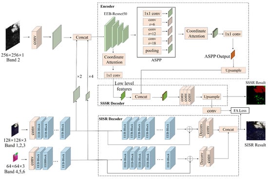
Figure 1.
Structure of the DSRSS-Net network. The abbreviations used are as follows. DSRSS-Net is the dual-branch super-resolution semantic segmentation network. Conv is the convolutional layer. EEB is the edge enhancement block. SSSR, SISR, FA, and ASPP are semantic-segmentation super-resolution, single-image super-resolution, feature affinity, and atrous spatial pyramid pooling, respectively.
2.2.1. Edge Enhancement Block
Due to the difficulty of learning fine image structures, this paper is inspired by the edge-oriented convolution block (ECB) method [30] and improves it for the cloud–snow segmentation task, which was finally named the edge enhancement block (EEB). This module contains a basic 3 × 3 convolution and uses a pre-defined Sobel filter in the horizontal and vertical directions and a Laplacian filter to extract edge information. The computations of the EEB module and the output are shown in Equations (1) and (2). The structures of the EEB, EEB-ResBlock with added edge enhancement module, and EEB-BottleNeck are illustrated in Figure 2.
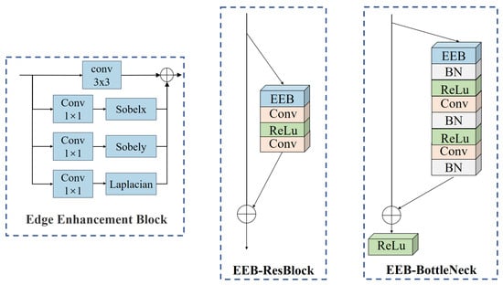
Figure 2.
Structures of the EEB, EEB-ResBlock, and EEB-BottleNeck.
2.2.2. Improved Coordinated Attention Module
The DeepLabv3+ model enlarges the model’s field of view through atrous spatial pyramid pooling (ASPP). However, the cloud and snow pixels in remote-sensing images have only small differences, which makes it difficult to distinguish features with high similarity by splicing the dimensional information of the shallow and deep layers, resulting in inaccurate cloud and snow classification. Therefore, an improved coordinated attention (CA) module [31] was added after the shallow feature output of the encoder and the deep feature output of the ASPP module to increase the distinction between different classes by assigning different weights to different channels to strengthen class features with strong correlations and suppress class features with weak correlations. The CA module uses average pooling to encode the input, taking the average value of the images in the pooling area and obtaining more sensitive background information to help with classification. Due to the high similarity between clouds and snow, average pooling leads to the mixing of feature information, which cannot effectively distinguish similar categories. Therefore, the CA module is improved by performing average pooling along with maximum pooling. Maximum pooling makes the feature map more sensitive to textural feature information, increasing the feature difference between clouds and snow and strengthening the classification effect between the two categories. The improved CA module structure is shown in Figure 3.
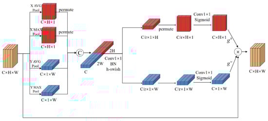
Figure 3.
Structure of the improved coordinated attention module. The abbreviations used are as follows. Conv is the convolutional layer followed by the kernel height × width. BN is batch normalization.
The first step is to perform average pooling and maximum pooling along the horizontal and vertical coordinates using pooling kernels and for the given feature map . The output of the channel at the height h can be represented as:
Similarly, the output of channel at width can be represented as:
The second step is to concatenate the output tensor, then pass it through shared 1 × 1 convolution to transform it to . denotes the downsampling step size, which is calculated as shown in Equation (7). After the nonlinear normalization calculation, f is split into two independent tensors and along the spatial dimension. Next, two 1 × 1 convolutions and are used to transform the two tensors into the same channel number as the input , and the sigmoid function is used to get and , as shown in Equations (8) and (9).
Finally, the attention weights matrix is obtained by matrix multiplication, and the output is expressed as (Equation (10)):
2.2.3. Multi-Task Loss Function
In the SISR branch, mean absolute error (MAE) loss is used (Equation (11)):
In the SSSR branch, cross-entropy loss (CE Loss) and boundary loss are used. CE loss is shown in Equation (12).
Boundary loss is a loss function for measuring boundary detection accuracy and penalizing wrong boundary segmentation. Firstly, maximum pooling with a sliding window size is used to extract the boundary, then the Euclidean distance from the pixel to the boundary is extracted. is set to be no more than the shortest distance in the ground truth map. Finally, the precision and recall are calculated as follows:
Finally, the boundary loss is represented as
Feature affinity loss can guide the segmentation branch to learn from the super-resolution branch, enabling the segmentation branch to benefit from the fine structural information in the super-resolution branch, thus obtaining more refined segmentation results.
where and are the similarity matrices of SSSR and SISR, respectively, and q is a norm and is set to 1 for the stability of training.
Finally, the multi-task loss of the network is composed of semantic segmentation loss, edge loss, super-resolution loss, and feature affinity loss in a linear combination.
3. Experiments
3.1. Experimental Environment Setting
The algorithm was implemented in the Ubuntu 18.04 operating system, with the deep learning framework PyTorch 1.10.0 and GPU acceleration tool CUDA 11.3 and the programming language Python 3.8. The hardware configuration included an i7-11700K CPU, Nvidia GeForce RTX 3090 GPU, and 128 GB memory. The dataset images were in TIF format, and the labels were in PNG format. Ten representative images of snow-covered areas with low cloud cover were selected to ensure that there were enough snow labels. The training set contained 10 FY-4 multispectral images. Each image was split into 275 image blocks, totaling 2750 images. The training set and test set were divided in an 8:2 ratio. During training, the batch size was set to 16, the number of iterations (Epoch) was set to 150, and an Adam optimizer was used to optimize the network, with an initial learning rate of 10–3.
3.2. Evaluation Metrics
This study uses overall accuracy (OA), mean intersection over union (MIoU), precision, recall, and F1-score (F1) to evaluate the model. OA denotes global accuracy and refers to the ratio of correctly predicted samples to all samples (Equation (19)). MIoU is the mean of all category IOUs, where IOU indicates the ratio of the intersection and union between ground truth and predictions (Equation (20)). Precision is the proportion of samples that were truly positive categories out of all samples that were categorized as positive categories (Equation (21)). Recall is the proportion of samples that were correctly classified as positive by the model out of all samples with actual positive categories (Equation (22)). F1 combines the accuracy of the model and its ability to find positive category samples; it is a weighted average of the precision and recall rates (Equation (23)).
Here, denotes the number of pixels that are correctly classified as the target, denotes the number of pixels that are neither the target nor the background, denotes the number of pixels that are misclassified as the background, denotes the number of pixels that are incorrectly classified as the target, and denotes the number of categories.
4. Results
4.1. Comparison of the Segmentation Models
Table 2 shows the comparison of segmentation indexes for different models, including UNet, DeepLabV3+, PSPNet [32], UNet++ [33], DenseASPP [34], CENet [28], and the proposed DSRSS-Net. The comparison was carried out on two sets of input data. The results show that when high-, medium-, and low-resolution inputs are combined, the segmentation results of all models are significantly better than those when only 2000 m low-resolution images are inputted alone. The performance indexes for the fully convolutional UNet model are the lowest due to the lack of sufficient context information. The PSPNet model adds the pooling pyramid structure, the CENet model applies the atrous convolution and multi-kernel pooling modules to the encoding–decoding structure, and the DenseASPP network uses densely connected spatial-pyramid pooling to obtain a larger field of view, but the segmentation accuracy is not improved significantly. This is because the difficulty of cloud–snow segmentation lies in the classification and boundary segmentation effects when clouds and snow are considerably mixed. The UNet++ model integrates different levels of image features by nesting subnetworks and long–short links and obtains higher MIoU and OA indexes, and its F1 index is only second to the model proposed in this paper. Compared with the other six models, the DSRSS-Net model first introduces the super-resolution branch and uses feature affinity loss to guide the semantic segmentation branch to learn fine structural information. Then, an improved coordinated attention mechanism is added to reduce the impact of irrelevant features after splicing on segmentation accuracy and improve classification accuracy for dense clouds and snow. Finally, the edge enhancement block and edge loss are used to improve boundary segmentation accuracy. As a result, our model obtains optimal detection results.
Table 2.
Comparison of different segmentation methods. The first set of input data is a single input from FY-4A/AGRI 2000 m resolution bands 1–6 (LR) and the second set of input data is a combination of FY-4A/AGRI 500 m resolution band-2 data (HR), 1000 m resolution band-1–3 data (MR), and 2000 m resolution band-4–6 data (LR).
To evaluate the snow and cloud segmentation results for different networks and the proposed DSRSS-Net, we used input data for different models composed of 500 m data and upsampled 1000 m and 2000 m data.
The results of cloud–snow detection for each model are shown in Figure 4. In addition to the six models mentioned above, this paper also adds a comparison with the MOD10A1 snow product. From the figure, it is easy to see that, due to the high similarity between clouds and snow, the other six models have recognition errors for cloud and snow recognition in the boundary areas. As for the processing of fragmented clouds and snow, except for the MOD10A1 product and UNet++, which fully aggregate different levels of features, the other models have a large number of missed detections. In terms of edge details, PSPNet’s processing of edges is particularly rough, and other models also have edge blurring. The DSRSS-Net proposed in this paper, on the other hand, incorporates an improved coordinated attention mechanism, which enables the network to better capture contextual information in the remote-sensing images, effectively mitigating the problem of cloud–snow misidentification and substantially improving the accuracy of cloud–snow recognition. On the other hand, we added an edge enhancement block in the residual module and BottleNeck, which made DSRSS-Net more refined in cloud–snow edge segmentation. Meanwhile, the improved coordinated attention mechanism, combined with the edge enhancement block, synergistically promotes the effectiveness of DSRSS-Net for fragmented cloud and snow recognition. Compared with the MOD10A1 snow product, MODIS carries a 500 m resolution sensor, and the model in this paper uses a combination of 500 m, 1000 m, and 2000 m data through super-resolution branching, which improves semantic segmentation accuracy. The accuracy of the cloud–snow extraction method is slightly lower than that of the MOD10A1 snow product but reaches the level of the 500 m snow product.
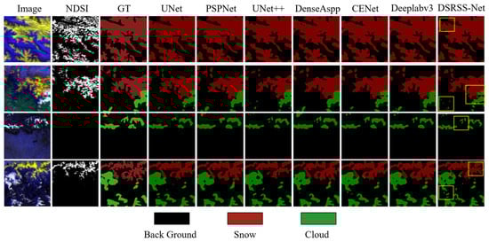
Figure 4.
Different cloud–snow segmentation effects. The images are FY-4A 500 m resolution images from bands 1, 2, and 5, synthesized from the super-resolution branch output results. NDSI is the 500 m resolution snow product MOD10A1, extracted using the NDSI snow thresholding method. GT is the 500 m resolution cloud and snow label.
As shown in Figure 5, we compared the extraction of FY-4A/AGRI snow data using the NDSI MOD10A1 snow product and the output of the super-resolution branch and semantic segmentation branch of the DSRSS-Net. It can be seen that the NDSI method is not sensitive to small snow spots or continuous snow blocks and lacks a large amount of snow recognition compared with the MOD10A1 snow product. The NDSI method only uses visible light and near-infrared bands for snow recognition, which is limited by the resolution of the 2000 m near-infrared band.
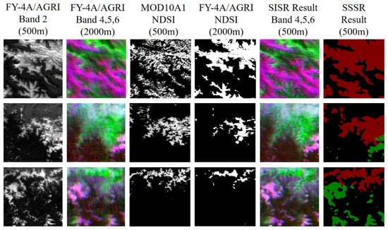
Figure 5.
Comparison between the super-resolution output and the semantic segmentation output.
4.2. Ablation Studies
To verify the effectiveness of each module for the super-resolution semantic segmentation proposed in this paper, we conducted ablation experiments on the super-resolution branch, improved coordinate attention mechanism, and edge enhancement block introduced into DSRSS-Net, as shown in Table 3. First, we replaced the improved coordinate attention mechanism and edge enhancement block with the classical coordinate attention mechanism and edge-oriented convolution block without adding the super-resolution branch, which was considered the base model. Then, we added the super-resolution branch to the base model to verify the effectiveness of the super-resolution branch. Then, we conducted three sets of ablation experiments according to the principle of removing or replacing one module in turn. Finally, each module proposed in this paper was added to the base model to obtain the final experimental results. The results show that, compared with the base model, each module contributes more to the improvement of cloud–snow detection. In this section, IOU, MioU, OA, Precision, Recall, and F1 are used as the main evaluation indexes.
Table 3.
Ablation experiments: SISR is the super-resolution decoder branch.
To obtain high-resolution detection results, this paper introduced the super-resolution decoder branch to provide rich structural information for semantic segmentation to guide high-resolution segmentation mapping and improve the edge segmentation effect by making the segmentation network obtain fine-grained structural information for the super-resolution branch through multi-task loss. The results show that the model introducing the super-resolution branch improves MioU and OA to 74.32% and 90.04%, which indicates that the super-resolution branch is effective in extracting spatial and semantic information.
The improved attention mechanism is used to enhance the differentiation between clouds and snow and increase the sensitivity of the network to feature map texture information, which in turn achieves the goal of improving the accuracy of cloud and snow classification. The results in Table 3 show that the improved attention mechanism is effective and can improve the MioU and OA of the model by 1.76% and 0.66%, respectively. In addition, the improved attention mechanism makes an important contribution to the improvement of metrics such as F1.
Due to the inconstant shapes and sizes of clouds and snow, the existing methods generated very rough boundaries and insufficient details. To repair edge details, we added the EEB to improve boundary segmentation accuracy. The EEB provides a greater enhancement of the edges compared with the classical ECB module, which improves the MioU and OA of the model by a further 0.54% and 0.25%.
4.3. Comparison of Snow Cover Mapping on the Qinghai–Tibet Plateau
The model proposed in this paper was used to classify and map snow cover in the Qinghai–Tibet Plateau region. The results are compared with the MOD10A1 snow product and the NDSI method. The results are shown in Figure 6. It was found that the NDSI snow retrieval method misses a large amount of snow, while the snow edge with DSRSS-Net is clear and accurate. The reason is that DSRSS-Net uses a combination of different bands as input to improve the spatial resolution of snow products. The MOD10A1 snow product has a spatial resolution of 500 m due to its sensor, so the snow outline is clear. However, with the limitation of it only providing a single daily image, there is potential for mistakenly identifying a large snowy area as cloud. In the above comparison, the DSRSS-Net snow recognition effect is the best, which shows that this method effectively makes up for the low spatial resolution of geostationary satellites relative to polar satellites and improves the recognition effect of the geostationary satellite snow product.
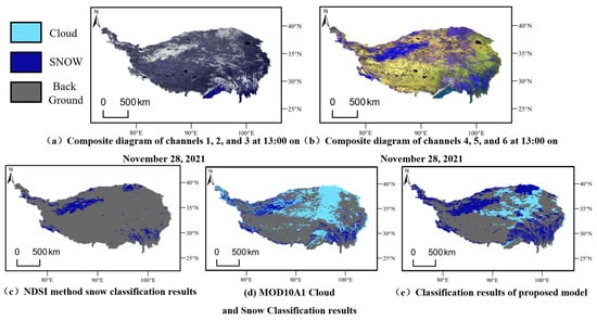
Figure 6.
Comparison of mappings of snow accumulation on the Qinghai–Tibet Plateau at 13:00 GMT on 28 November 2021: (a) is a composite image of the FY-4A 500 m resolution output from bands 1, 2, and 3 from the super-resolution branch; (b) is composite image of the FY-4A 500 m resolution output from bands 4, 5, and 6 from the super-resolution branch; (c) is FY-4A 500 m resolution imagery extracted using NDSI; (d) is the result of cloud and snow classification with MOD10A1 at a 500 m resolution; and (e) is the result of cloud and snow classification for the proposed model at 500 m resolution.
4.4. Verification against a Ground Weather Station
The snow depth data from 95 meteorological stations in the Qinghai–Tibet Plateau from January to March 2020 were collected and compared with the snow classification accuracy, false detection rate, and total classification accuracy for the MOD10A1 and DSRSS-Net snow products. As shown in Equation (24), snow classification accuracy denotes the ratio of the number of samples correctly identified as snow points to the number of samples with snow points in ground meteorological stations. As shown in Equation (25), the snow false-alarm rate Os denotes the ratio of the number of samples identified as snow without snow identified by ground meteorological stations to the number of samples without snow . As shown in Equation (26), the total classification accuracy denotes the ratio of the number of correctly identified snow points and non-snow points to the number of ground meteorological stations .
In the verification process, to objectively reflect the accuracy of snow cover products, data from meteorological stations that are covered by clouds is usually not used to validate accuracy in the prevailing ground station verification method. Additionally, to prevent the sample size from being too small and losing statistical significance, if there are too many stations recording clouds on a certain day and the number of meteorological stations that are not covered by clouds is less than 30, the data from that day is not counted in the weekly average accuracy rate. This paper statistically verifies the weekly average snow classification accuracy, false detection rate, and total classification accuracy for 13 weeks from January to March 2020 (Figure 7).
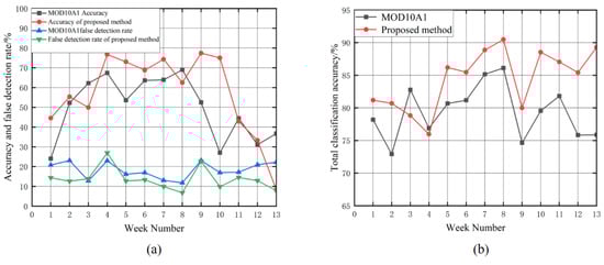
Figure 7.
Detection rate comparison for snow classification from January to March 2020. Figure (a) shows the accuracy and false detection rate of the proposed model and the MOD10A1 snow product. Figure (b) shows the total classification accuracy of the proposed model and the MOD10A1 snow product.
The time recorded by ground meteorological stations is fixed and there is a time difference with the transit time of the MODIS satellite. Using ground truth values to verify satellite inversion data may result in errors. Therefore, from Figure 7a, it can be seen that, due to frequent temperature changes in the Qinghai–Tibet Plateau, the accuracy of MOD10A1 snow classification in the first week has significantly decreased due to repeated melting and accumulation of snow cover. The snow cover classification accuracy of DSRSS-Net in the 13th week also decreased significantly due to the uneven distribution of meteorological stations in the Qinghai–Tibet Plateau, most of which are distributed in the eastern region, and this week’s cloud cover was large. The true snow cover sample in the FY-4A data was severely obscured by clouds, resulting in the classification accuracy for this week not having an objective comparison. As shown in Table 4, the average accuracy for snow cover in January–March 2020 was 55.14%, the average total accuracy was 84.46%, and the average false-alarm rate was 13.70%, which are all better than that of the MODIS snow cover product. Thus, compared with ground meteorological stations, the DSRSS-Net snow cover classification effect is better than that of the MODIS snow cover product.
Table 4.
Snow detection accuracy of the MOD10A1 product and the proposed model from January to March 2020.
4.5. Mask Verification
To further validate the accuracy of the snow detection results from the model proposed in this paper, we selected four images at different times, such as 2 March 2017 and 6 August 2019, to validate the results of this paper with the results from Landset8 images detected using the snow map algorithm, as shown in Figure 8. It should be noted that, here, we only performed the validation of snow detection, and to emphasize the contrast effect we classified the clouds in the output results of the model proposed in this paper as the background.
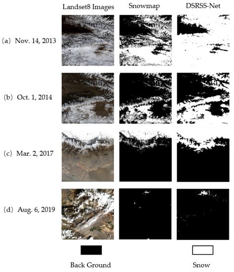
Figure 8.
Landset8 mask verification: Landset8 images are the Landset8 30 m resolution raw images; Snowmap is the result of snow detection through Landset8 raw images using the Snowmap algorithm; DSRRS-Net is the result of snow detection for the model proposed in this paper.
From the figure, it can be seen that the model in this paper has relatively high detection accuracy for snow-rich regions and can maintain clear edge information as shown in Figure 8a,b. However, due to the limitation of resolution, there is adhesion in the detection of fragmented snow causing false detection. As can be seen from Figure 8c, in mountainous areas with complex terrain, the model proposed in this paper can reflect the real snow features more clearly compared with the Snowmap algorithm. On the other hand, in the case of cloud occlusion, the snow detection of the model proposed in this paper suffers from the problem of cloud interference. As shown in Figure 8d, there are not only missed detections but also sporadic false detections.
5. Conclusions
In this paper, an end-to-end dual-branch super-resolution semantic segmentation network was proposed for snow recognition in the Tibetan Plateau region. The network was improved based on the Deeplabv3+ framework by adding an image super-resolution decoder branch, utilizing super-resolution branch information containing rich structural information to guide high-resolution segmentation mapping, and improving classification performance and the edge segmentation effect for cloud and snow by combining an edge-enhancing block and coordinated attention mechanism.
The experimental results show that DSRSS-Net obtains high-accuracy 500 m cloud–snow discrimination results, and the improved CA module substantially alleviates the problem of cloud–snow misclassification. In addition, the addition of the edge enhancement module enables DSRSS to obtain more accurate edges in segmentation and also improves its sensitivity to small snow patches and continuous snow blocks. DSRSS-Net outperforms other classical segmentation networks in terms of all evaluation metrics. Compared with MOD10A1, DSRSS-Net improves snow classification accuracy and average total accuracy by 4.45% and 5.1%, respectively.
Although the model proposed in this paper has achieved good results, it still falls short of satellites equipped with high-resolution sensors due to the limitations of the satellites’ sensors. In the future, on the one hand, it is expected that data quality can be improved by combining it with other high-resolution satellite images; on the other hand, we will try to incorporate spatiotemporal and topographic factors into the input data, improve the network structure, and further improve the accuracy of cloud and snow recognition.
Author Contributions
Conceptualization, X.K. and L.Z.; methodology, X.K.; software, Z.L.; validation, X.K., Z.L. and L.Z.; formal analysis, Z.L.; investigation, L.Z.; resources, Y.Z.; data curation, L.Z.; writing—original draft preparation, X.K. and Z.L., writing—review and editing, X.K., Z.L., L.Z., X.L., Z.Z. and K.T.C.L.K.S., visualization, L.Z., H.C. and J.W.; supervision, X.K.; project administration, X.K. and Y.Z.; funding acquisition, X.K. and Y.Z. All authors have read and agreed to the published version of the manuscript.
Funding
This research was funded by the National Natural Science Foundation of China, grant numbers 42105143 and 42305158, the Natural Science Foundation of the Jiangsu Higher Education Institutions of China, grant numbers 21KJB170006 and 23KJB170025, the National Key Research and Development Program of China, grant number 2021YFE0116900, and the Research Start-up Fund of Wuxi University, grant number 2022r035.
Data Availability Statement
The data supporting the findings of this study are available from the first author (X.K.).
Acknowledgments
We are immensely grateful to the editor and anonymous reviewers for their comments on the manuscript. The authors would like to thank Ya Chu for her help with data acquisition.
Conflicts of Interest
The authors declare no conflict of interest.
References
- Jin, Z.; You, Q.L.; Wu, F.Y. Characteristics of climate and extreme climate change in Sanjiangyuan region of Qinghai-Tibet Plateau during the past 60 years. J. Atmos. Sci. 2020, 43, 1042–1055. [Google Scholar]
- Hu, Y.; Zhang, Y.; Yan, L.; Li, X.-M.; Dou, C.; Jia, G.; Si, Y.; Zhang, L. Evaluation of the Radiometric Calibration of FY4A-AGRI Thermal Infrared Data Using Lake Qinghai. IEEE Trans. Geosci. Remote Sens. 2021, 59, 8040–8050. [Google Scholar] [CrossRef]
- Hall, D.K.; Riggs, G.A.; Salomonson, V.V. Development of methods for mapping global snow cover using moderate resolution imaging spectroradiometer data. Remote Sens. Environ. 1995, 54, 127–140. [Google Scholar] [CrossRef]
- Badrinarayanan, V.; Kendall, A.; Cipolla, R. Segnet: A deep convolutional encoder-decoder architecture for image segmentation. IEEE Trans. Pattern Anal. Mach. Intell. 2017, 39, 2481–2495. [Google Scholar] [CrossRef] [PubMed]
- Ronneberger, O.; Fischer, P.; Brox, T. U-net: Convolutional networks for biomedical image segmentation. In Medical Image Computing and Computer-Assisted Intervention–MICCAI 2015; Tal, A., Gustavo, C., Eds.; Springer: Cham, Switzerland, 2015; Part 3; pp. 234–241. [Google Scholar]
- Chen, L.C.; Papandreou, G.; Schroff, F. Rethinking atrous convolution for semantic image segmentation. In Proceedings of the International Conference on Computer Vision and Pattern Recognition, Honolulu, HI, USA, 21–26 July 2017. [Google Scholar]
- Lee, S.H.; Han, K.J.; Lee, K. Classification of landscape affected by deforestation using high-resolution remote sensing data and deep-learning techniques. Remote Sens. 2020, 12, 3372. [Google Scholar] [CrossRef]
- Parente, L.; Taquary, E.; Silva, A.P. Next generation mapping: Combining deep learning, cloud computing, and big remote sensing data. Remote Sens. 2019, 11, 2881. [Google Scholar] [CrossRef]
- Dong, C.; Loy, C.C.; He, K. Image super-resolution using deep convolutional networks. IEEE Trans. Pattern Anal. Mach. Intell. 2015, 38, 295–307. [Google Scholar] [CrossRef] [PubMed]
- Dong, C.; Loy, C.C.; He, K. Learning a deep convolutional network for image super-resolution. In European Conference on Computer Vision; Tal, A., Gustavo, C., Eds.; Springer: Cham, Switzerland, 2014; pp. 184–199. [Google Scholar]
- Dong, C.; Loy, C.C.; Tang, X. Accelerating the super-resolution convolutional neural network. In European Conference on Computer Vision; Tal, A., Gustavo, C., Eds.; Springer: Cham, Switzerland, 2016; pp. 391–407. [Google Scholar]
- Shi, W.; Caballero, J.; Huszár, F. Real-time single image and video super-resolution using an efficient sub-pixel convolutional neural network. In Proceedings of the 2016 IEEE Conference on Computer Vision and Pattern Recognition (CVPR), Las Vegas, NV, USA, 27–30 June 2016; IEEE: Piscataway, NJ, USA, 2016; pp. 1874–1883. [Google Scholar]
- Kim, J.; Lee, J.K.; Lee, K.M. Accurate image super-resolution using very deep convolutional networks. In Proceedings of the 2016 IEEE Conference on Computer Vision and Pattern Recognition (CVPR), Las Vegas, NV, USA, 27–30 June 2016; IEEE: Piscataway, NJ, USA, 2016; pp. 1646–1654. [Google Scholar]
- Lim, B.; Son, S.; Kim, H.; Nah, S.; Mu Lee, K. Enhanced deep residual networks for single image super-resolution. In Proceedings of the 2017 IEEE Conference on Computer Vision and Pattern Recognition Workshops (CVPRW), Honolulu, HI, USA, 21–26 July 2017; IEEE: Piscataway, NJ, USA, 2017; pp. 136–144. [Google Scholar]
- Sajjadi, M.S.; Scholkopf, B.; Hirsch, M. Enhancenet: Single image super-resolution through automated texture synthesis. In Proceedings of the 2017 IEEE International Conference on Computer Vision (ICCV), Venice, Italy, 22–29 October 2017; IEEE: Piscataway, NJ, USA, 2017; pp. 4491–4500. [Google Scholar]
- Wang, X.; Yu, K.; Wu, S. Esrgan: Enhanced super-resolution generative adversarial networks. In Proceedings of the European Conference on Computer Vision (ECCV) Workshops, Munich, Germany, 8–14 September 2018; Springer: Cham, Switzerland, 2018. [Google Scholar]
- Zhang, K.; Sumbul, G.; Demir, B. An approach to super-resolution of sentinel-2 images based on generative adversarial networks. In Proceedings of the 2020 Mediterranean and Middle-East Geoscience and Remote Sensing Symposium (M2GARSS), Tunis, Tunisia, 9–11 March 2020; IEEE: Piscataway, NJ, USA, 2020; pp. 69–72. [Google Scholar]
- Chen, B.; Li, J.; Jin, Y. Deep learning for feature-level data fusion: Higher resolution reconstruction of historical landsat archive. Remote Sens. 2021, 13, 167. [Google Scholar] [CrossRef]
- Dai, D.; Wang, Y.; Chen, Y. Is image super-resolution helpful for other vision tasks? In Proceedings of the 2016 IEEE Winter Conference on Applications of Computer Vision (WACV), Lake Placid, NY, USA, 7–10 March 2016; IEEE: Piscataway, NJ, USA, 2016; pp. 1–9. [Google Scholar]
- Guo, Z.; Wu, G.; Song, X. Super-resolution integrated building semantic segmentation for multi-source remote sensing imagery. IEEE Access 2019, 7, 99381–99397. [Google Scholar] [CrossRef]
- Lei, S.; Shi, Z.; Wu, X.; Pan, B.; Xu, X.; Hao, H. Simultaneous super-resolution and segmentation for remote sensing images. In Proceedings of the IGARSS 2019—2019 IEEE International Geoscience and Remote Sensing Symposium, Yokohama, Japan, 28 July–2 August 2019; IEEE: Piscataway, NJ, USA, 2019; pp. 3121–3124. [Google Scholar]
- Wang, L.; Li, D.; Zhu, Y.; Tian, L.; Shan, Y. Dual super-resolution learning for semantic segmentation. In Proceedings of the 2020 IEEE/CVF Conference on Computer Vision and Pattern Recognition (CVPR), Seattle, WA, USA, 13–19 June 2020; IEEE: Piscataway, NJ, USA, 2020; pp. 3774–3783. [Google Scholar]
- Xu, P.L.; Tang, H.; Ge, J.Y.; Feng, L. ESPC_NASUnet: An End-to-End Super-Resolution Semantic Segmentation Network for Mapping Buildings from Remote Sensing Images. IEEE J. Sel. Top. Appl. Earth Obs. Remote Sens. 2021, 14, 5421–5435. [Google Scholar] [CrossRef]
- Abadal, S.; Salgueiro, L.; Marcello, J. A dual network for super-resolution and semantic segmentation of sentinel-2 imagery. Remote Sens. 2021, 13, 4547. [Google Scholar] [CrossRef]
- Jiang, J.; Liu, L.; Fu, J.; Wang, W.N.; Lu, H.Q. Super-resolution semantic segmentation with relation calibrating network. Pattern Recognit. 2022, 12, 108501. [Google Scholar] [CrossRef]
- Zhang, Y.H.; Cai, P.Y.; Tao, R.C. Remote sensing image cloud detection based on improved U-Net network. J. Surv. Mapp. Bull. 2020, 3, 17–20. [Google Scholar]
- Lu, Z.H.; Kan, X.; Li, Y. Super-resolution reconstruction of Fengyun-4 satellite images based on matching extraction and cross-scale feature fusion network. J. Adv. Lasers Optoelectron. 2023, 60, 128–138. [Google Scholar]
- Gu, Z.; Cheng, J.; Fu, H. Ce-net: Context encoder network for 2d medical image segmentation. IEEE Trans. Med. Imaging 2019, 38, 2281–2292. [Google Scholar] [CrossRef] [PubMed]
- Tong, R.; Parajka, J.; Komma, J.; Blöschl, G. Mapping snow cover from daily Collection 6 MODIS products over Austria. J. Hydrol. 2020, 590, 125548. [Google Scholar] [CrossRef]
- Zhang, X.D.; Zeng, H.; Zhang, L. Edge-oriented Convolution Block for Real-time Super Resolution on Mobile Devices. In Proceedings of the 29th ACM International Conference on Multimedia, Chengdu, China, 20–24 October 2021; Association for Computing Machinery: New York, NY, USA, 2021; pp. 4034–4043. [Google Scholar]
- Hou, Q.; Zhou, D.; Feng, J. Coordinate attention for efficient mobile network design. In Proceedings of the 2021 IEEE/CVF Conference on Computer Vision and Pattern Recognition (CVPR), Nashville, TN, USA, 20–25 June 2021; IEEE: Piscataway, NJ, USA, 2021; pp. 13713–13722. [Google Scholar]
- Zhao, H.; Shi, J.; Qi, X. Pyramid scene parsing network. In Proceedings of the 2017 IEEE Conference on Computer Vision and Pattern Recognition (CVPR), Honolulu, HI, USA, 21–26 July 2017; IEEE: Piscataway, NJ, USA, 2017; pp. 2881–2890. [Google Scholar]
- Zhou, Z.; Rahman, S.M.M.; Tajbakhsh, N. Unet++: A nested u-net architecture for medical image segmentation. In Deep Learning in Medical Image Analysis and Multimodal Learning for Clinical Decision Support; Tal, A., Gustavo, C., Eds.; Springer: Cham, Switzerland, 2018; Volume 4, pp. 3–11. [Google Scholar]
- Yang, M.; Yu, K.; Zhang, C. Denseaspp for semantic segmentation in street scenes. In Proceedings of the 2018 IEEE/CVF Conference on Computer Vision and Pattern Recognition, Salt Lake City, UT, USA, 18–23 June 2018; IEEE: Piscataway, NJ, USA, 2018; pp. 3684–3692. [Google Scholar]
Disclaimer/Publisher’s Note: The statements, opinions and data contained in all publications are solely those of the individual author(s) and contributor(s) and not of MDPI and/or the editor(s). MDPI and/or the editor(s) disclaim responsibility for any injury to people or property resulting from any ideas, methods, instructions or products referred to in the content. |
© 2023 by the authors. Licensee MDPI, Basel, Switzerland. This article is an open access article distributed under the terms and conditions of the Creative Commons Attribution (CC BY) license (https://creativecommons.org/licenses/by/4.0/).