Impact of a Hyperspectral Satellite Cross-Calibration Radiometer’s Spatial and Noise Characteristics on Cross-Calibration

Abstract

The satellite cross-calibration radiometer (SCR) is a conceptual on-orbit hyperspectral imaging radiometer that transfers the radiometric calibration from a “gold-standard” reference instrument such as the Landsat 8/9 Operational Land Imager (OLI) to other civil, international, or commercial “client” multispectral satellite systems via near-simultaneous cross-calibration acquisitions. The spectral resolution, spectral range, spatial resolution, and signal-to-noise ratio (SNR) all significantly impact the complexity and cost of hyperspectral SCRs, so it is important to understand their effect on cross-calibration quality. This paper discusses the results of a trade study to quantify the effects of varying ground sample distance (GSD), number of independent samples, and instrument/scene noise on cross-calibration gain uncertainties. The trade study used a simulated SCR cross-calibration with near-simultaneous nadir overpasses (SNOs) of the Landsat 8 OLI acting as the reference instrument and the DLR Earth Sensing Imaging Spectrometer (DESIS) acting as a surrogate SCR hyperspectral instrument. Results demonstrate that cross-calibration uncertainty is only minimally affected by spatial resolution and SNR, which may allow SCR instruments to be developed at a lower cost.

1. Introduction

Earth-viewing remote sensing satellite instruments need accurate radiometric calibration to determine surface reflectance properties and perform long-term time series monitoring and analysis. While many large satellites have onboard calibrators such as lamps, solar diffusers, and black bodies for ensuring accurate radiometry, the complexity, size, weight, and power constraints of these onboard calibration components prevent most small satellites from incorporating them. Smaller satellite systems instead rely on vicarious methods and potentially near-simultaneous nadir overpass (SNO)-based cross-calibrations with well-calibrated systems, to achieve accurate calibration. Near-simultaneous cross-calibrations however, require a method to correct for spectral bandpass differences between sensors. The hyperspectral satellite cross-calibration radiometer (SCR) addresses this issue using a technique known as spectral synthesis, whereby client and gold-standard multispectral bands are synthesized from multiple fine-resolution overlapping hyperspectral bands. As with other satellite instruments, the SCR’s ultimate performance, size, and cost depend on its signal-to-noise ratio (SNR) and spatial and spectral characteristics. A reasonable goal for the SCR is to transfer the radiometric calibration to a client satellite imager with ~1% or better transfer calibration uncertainty under ideal near-SNO conditions. At this level of transfer uncertainty, there will be a minimal increase in current land imager SI uncertainty, which is generally, over land, on the order of 3–5%, for well-calibrated remote sensing systems like the Landsat 8 (L8) and Sentinel-2 (S-2) [1,2].

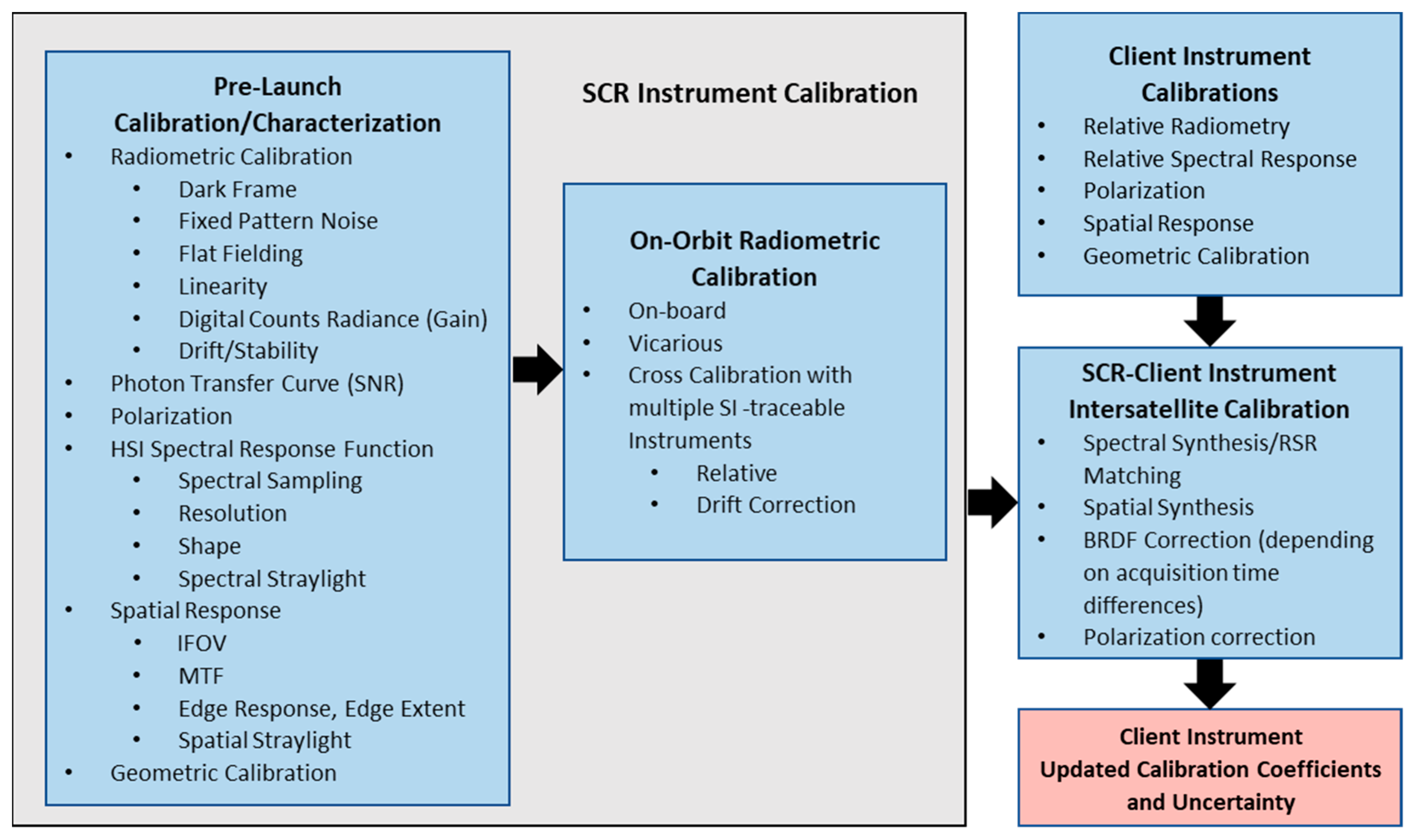
The SCR is assumed to be well-calibrated, stable, and highly characterized to meet this radiometric transfer uncertainty goal, as described in Figure 1. Thorough pre-launch SCR laboratory-based measurements are critical and should include: radiometric and geometric calibrations including full dark frame measurements; spectral and spatial response measurements; photon transfer curve measurements; and polarization sensitivity measurements. After launch, regularly occurring on-orbit radiometric calibrations, including those using any onboard sources and vicarious methods, as well as cross-calibrations with multiple well-calibrated SI-traceable systems that track drift, and that are preferably hyperspectral, should also be performed. Cross-calibrations can then be performed between the well-calibrated and monitored SCR and client instruments to transfer the radiometric calibration back to the client instrument. Cross-calibrations between the reference instrument and the SCR, and between the client instrument and the SCR are performed in a similar fashion.

Several SCR characteristics that impact instrument and satellite design, including spatial, spectral, and SNR parameters, are highlighted in

Table 1. Sensor Parameters that Impact SCR Designs.

Parameter	General Impact on Design
GSD	Smaller GSD increases data volume. May require higher data rates. Larger GSD decreases focal length and fore-optic size and increases exposure times, sensitivity, and possibly SNR. May have limited use of RadCalNet sites if GSD becomes too large.
Swath	Decreased swath minimizes the impact of the bidirectional reflectance distribution function (BRDF) and uses smaller FPAs.
Spectral	Spectral sampling and resolution must be fine enough to simulate the reference and client instrument’s spectral properties. Spectral range must cover the wavelength region of interest.
SNR	SNR can be relaxed since cross-calibration regression with many points improves the precision of gain (and offset when required) estimates.

. Because the focal length of an optical system, which is inversely proportional to its ground sample distance (GSD), increases the instrument’s weight, size, and resulting output data volume, an SCR with a larger GSD is highly desirable. Similarly, with a fixed f-number system, since a telescope’s aperture diameter also scales inversely with GSD, the telescope’s volume and mass scale approximately inversely with GSD³. For example, an optical system with a GSD 10× larger than another might have a telescope with ~1000× smaller volume and mass. Also, by having a larger GSD with an equivalent swath, an SCR could use focal plane arrays (FPAs) with fewer pixels, reducing power consumption and cost. A downside of a large GSD, however, is that it limits the use of calibration sites such as instrumented Radiometric Calibration Network (RadCalNet) sites, which range in size from 45 m × 45 m up to 1 km × 1 km [3].

The SNR required for an SCR is not as high as what is required for traditional hyperspectral instruments used for spectral analysis algorithms, but is still a consideration, especially for low illumination conditions near the poles. The SNR increases with larger apertures, or smaller f-numbers, and longer exposure times. Larger GSDs collect more light and enable longer integration times. In a pushbroom system operating at a constant orbital speed, exposure times approximately scale with GSD, so in a photon-noise-limited case, SNR scales by the GSD^3/2.

In order to minimize spectral synthesis matching errors, an SCR’s spectral sampling must be sufficiently high. These matching errors are small and less than 0.5% if the hyperspectral sampling interval is several times finer than the multispectral (reference or client) instrument’s relative spectral response (RSR) full width at half maximum (FWHM). Relative radiometry errors, such as flat fielding, linearity, stability, etc., must also be much smaller than 1%.

This paper discusses the results of a trade study that was performed to quantify the effects of varying GSD, SNR, and sample size on cross-calibration gain uncertainties by simulating an SCR cross-calibration using near-SNOs with the L8 Operational Land Imager (OLI) acting as the reference instrument and the German Aerospace Center (DLR) Earth Sensing Imaging Spectrometer (DESIS) acting as a surrogate SCR hyperspectral instrument. The scope of this paper is limited to the uncertainties associated with cross-calibration.

1.1. Current State of the Art

At present, the radiometric quality of data from many civil and commercial satellites varies and for satellites without onboard calibration, the radiometric accuracy is heavily dependent on vicarious calibration. Comparing data acquired at different times from the same satellite can also be challenging if there is drift, which is difficult to track without frequent calibration. These uncertainties significantly diminish the scientific value of the systems that lack on-board calibration, for various applications, including climate change, agriculture, geology, and hydrology. SI-traceable satellites (SITSATS), including the National Aeronautics and Space Administration’s (NASA’s) Climate Absolute Radiance and Refractivity Observatory (CLARREO) Pathfinder (CPF), the National Physical Laboratory’s (NPL’s) Cryogenic Solar Absolute Radiometer (CSAR), and the United Kingdom Space Agency’s (UKSA’s) Traceable Radiometry Underpinning Terrestrial- and Helio-Studies (TRUTHS) instruments are currently being planned to meet these challenging application needs [4]. NPL’s CSAR is predicted to be SI-traceable to 0.1% [4] and CPF has an expected radiometric uncertainty of 0.3%, significantly better than current remote sensing satellites. SCR cross-calibration with these types of reference sensors may become possible, increasing the availability of radiometrically accurate data from many satellites.

In light of these SI-traceable on-orbit transfer radiometers’ potential benefits, there has been increasing interest in applying methods similar to those proposed with SITSATS, using less advanced hyperspectral technology to dramatically improve client remote sensing systems’ calibrations at a significantly reduced cost [5]. Even an SCR instrument with an absolute SI radiometric accuracy of 3–5% could significantly improve other instrument calibrations and provide increased confidence in them. While a detailed discussion of SCR calibration and SI-traceability is beyond the scope of this study, it is assumed that the instrument is well characterized on the ground prior to launch and has a robust on-orbit calibration mechanism in place. Ideally, the SCR will carry an onboard calibrator, but with the use of vicarious calibration methods and cross-calibration with other instruments, the SCR, following other remote sensing systems, should achieve 3–5% absolute radiometric accuracies without it [3]. Because cost and technical limitations inhibit the SCR’s potential accuracy, it is necessary to understand how SCR data properties (i.e., spatial, spectral, and SNR) impact the uncertainty of cross-calibrations between an SCR and a reference instrument.

1.1.1. DESIS

The DLR Earth Sensing Imaging Spectrometer (DESIS) is a visible through near-infrared (NIR) hyperspectral instrument resulting from a collaboration between Teledyne Brown Engineering and DLR. DESIS was chosen as a surrogate SCR because its spectral capabilities are comparable to reference calibration satellites such as CPF and TRUTHS and because it has a light emitting diode (LED)-based onboard calibration unit. DESIS is a hyperspectral instrument with 235 bands in the visible–NIR range. It was mounted on the International Space Station (ISS) via the Multi-User System for Earth Sensing (MUSES) platform in 2018. While it had an originally projected mission design lifetime of five years [6], it is anticipated to operate longer than this design life. DESIS’ onboard calibration is regularly updated using vicarious calibration methods and RadCalNet sites.

Table 2. Relevant DESIS Parameters.

Parameter	Values
Spectral Range (nm)	400–1000
GSD (m)	30
MTF@Nyquist	>20%
FWHM (nm)	<3
Spectral Sampling (nm)	2.55
SNR@550 nm	195 with no binning 386 when binning 4 bands (At conditions of albedo 0.3, 45° SZA)

lists DESIS’ parameters most relevant to this study [6]. The SNR value, shown in the table, was calculated for the 550 nm band using 0.3 albedo at a 45° solar zenith angle (SZA) [7].

1.1.2. Landsat 8 OLI

L8 launched in 2013, and has two multispectral sensors: the Operational Land Imager (OLI), which operates in the visible through shortwave infrared spectral region, and the Thermal Infrared Sensor (TIRS), which operates in the thermal infrared. It is the first pushbroom sensor in the Landsat series. This study selected L8 OLI as the reference instrument due to its gold standard SI-traceable absolute calibrations [8,9]. It also collects imagery globally, making it possible to identify many near-coincident collections with DESIS.

Table 3. Relevant L8 OLI Parameters.

Parameter	Values
Spectral Range (nm)	400–2500 (OLI)
GSD (m)	30 (Coastal, Blue, Green, Red, NIR)
Center Wavelength (nm)	443 (Coastal), 482 (Blue), 562 (Green), 655 (Red), 865 (NIR)
Bandwidth (nm)	20 (Coastal), 65 (Blue), 75 (Green), 50 (Red), 40 (NIR)
SNR at typical radiance	237 (Coastal), 367 (Blue), 304 (Green), 227 (Red), 201 (NIR)

shows the specifications for the L8 OLI most relevant to this study [10]. The per-band SNR values were measured on-orbit at L8 typical radiance levels (L_typ) [11].

1.1.3. Differences between Cross-Calibration and Traditional Vicarious Calibration

Traditional vicarious calibrations require taking ground truth measurements using well-calibrated instruments coincident with a satellite observation. Ground truth measurements include ground surface reflectance and atmospheric measurements. The atmospheric measurements are used to propagate ground surface reflectance measurements to estimate satellite-acquired top-of-atmosphere (TOA) values. Calibrations are performed by comparing estimated TOA values with the satellite-acquired values. Uncertainties with this approach include uncertainties in the radiative transport model and exo-atmospheric solar irradiance estimate. Vicarious calibration sites are well known and understood and they are typically relatively bright, producing reflectance values at the higher end of a sensor’s dynamic range. Bright sites reduce the influence of the atmosphere, which is the highest contributor to uncertainty. This type of calibration often produces a single point measurement and assumes that the system being calibrated is linear. Ground surface measurements are taken over a finite area, typically spanning less than hundreds of pixels [12,13].

By comparison, a cross-calibration with an SI-traceable reference system requires that the target and reference system acquire imagery over the same location at the same time. While not consistently defined in the literature, the term near-SNO is used to restrict the inter-acquisition time gap (IATG), and temporal and viewing geometry differences between sensor acquisitions. Temporal differences affect solar geometry, important for BRDF, and the possibility of different atmospheres being present between the two acquisitions. Near-nadir geometries are usually chosen. Cross-calibrations are performed by comparing the top-of-atmosphere (TOA) values on a pixel-by-pixel basis through regression, and therefore do not contain atmospheric modeling uncertainties. Significant overlap between the two sensors provide an opportunity to compare millions of pixels, and as uncertainty decreases with the square root of the number of independent samples, cross-calibration has the ability to produce high confidence results. Cross-calibration scenes are not limited to the handful of instrumented sites used in vicarious calibrations, and properly chosen scenes can produce at-sensor radiance values that span the dynamic range of a sensor [14,15].

An SCR that has undergone extensive pre-launch calibrations (Figure 1), that maintains its calibration through on-board calibrators and cross-calibrations with SI-traceable sensors, can be used to transfer its calibration to client satellites via separate cross-calibrations.

2. Materials and Methods

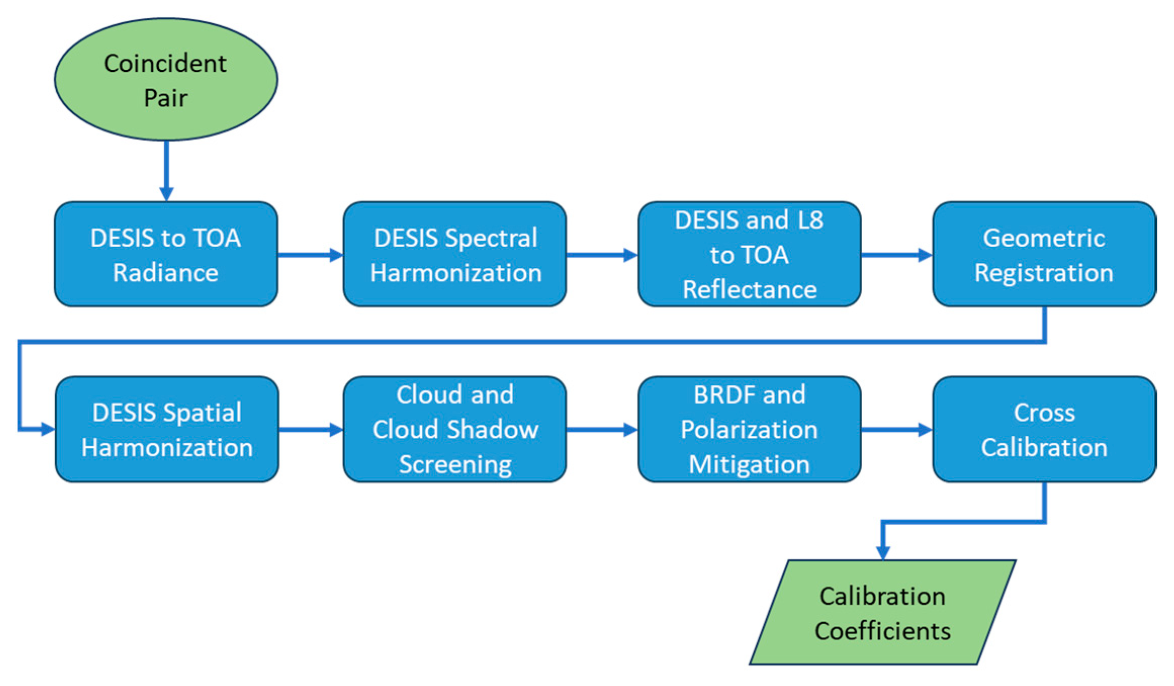
The steps used to perform a notional cross-calibration between an SCR and a reference satellite are highlighted in Figure 2 and shown in closer detail in the sections below and within [16]. In this study, the DESIS hyperspectral sensor is used as an SCR surrogate and L8 is used as the reference satellite.

2.1. Near-Coincident Cross-Calibration

Cross-calibration typically begins with identifying collections over a common region that are nearly simultaneous and have either similar viewing geometries or a way to correct for these differences. This reduces the impact of atmospheric, illumination, BRDF, cloud cover, and/or land cover changes between scenes [14,15]. Using sufficiently large uniform regions found at most RadCalNet sites [3] and all pseudo-invariant calibration (PIC) sites [17] reduces the significance of different instruments’ spatial properties. These sites provide relatively unchanging Earth surfaces (usually deserts) that facilitate monitoring satellite accuracy over time [3,18]. Unfortunately, they also have reflectance values at the high end of a sensor’s dynamic range, which may mask straylight and linearity problems. To reduce the effects of this limitation, cross-calibrations using multiple scene pairs over varied land covers were used for this study.

2.2. Identification of Near-Coincident Collects

Suitable DESIS imagery was located by searching the DESIS TCloud imagery catalog (https://teledyne.tcloudhost.com/) (accessed on 3 August 2023). Images over a variety of land covers, filtered to include only imagery labeled with a cloud cover statistical designation of “clear” were identified, meaning that a visual inspection of the DESIS image revealed no clouds were present in the scene. A Python script was developed to search the results to identify near-coincident Landsat collects. The script filtered L8 imagery by time, eliminating imagery taken more than 3.5 min apart from DESIS imagery. As Landsat includes a cirrus band, not present in DESIS, the Landsat QA band was also reviewed to ensure a completely cloud-free image was selected. The near-coincident image pairs were also filtered to limit view zenith angles to less than 7°. While these filtering values are arbitrary, and within the bounds of commonly used near-SNO parameters [14,15,19,20], they represent reasonable parameters and produced eleven L8/DESIS image pairs, shown in

Table 4. DESIS/L8 Cross-calibration Sites.

Location	L8 Path/Row	DESIS Tile	Date	Time Diff. (min:s)	View Azimuth Diff. (deg)	View Zenith Diff. (deg)
Corona, NM	033/036	1	28 August 2020	3:27	37.90	2.15
Oklahoma	027/037	2	8 December 2020	1:42	59.52	5.66
Oklahoma	027/036	8	8 December 2020	2:33	214.80	2.47
Oklahoma	027/035	11	8 December 2020	3:09	233.25	6.79
Paraguay	225/077	3	9 March 2021	3:27	27.49	4.17
Paraguay	225/078	7	9 March 2021	3:21	154.08	3.90
Egypt 1	178/042	11	29 December 2021	0:18	84.43	0.53
Egypt 1	178/043	14	29 December 2021	0:08	148.71	5.52
Mauritania 2	201/045	33	30 December 2021	3:03	24.95	2.01
Mauritania 2	201/046	37	30 December 2021	3:10	126.04	0.86
Snow Mt, CA	044/032	7	9 April 2022	0:36	41.61	3.04

. The identified scenes were downloaded from TCloud (DESIS) or USGS Earth Explorer (L8). DESIS data sets were processed to Level 1C, a TOA orthorectified radiance product [21]. Landsat imagery was processed to Level1TP, a precision terrain-corrected orthorectified product [22], and converted to TOA reflectance using associated metadata. While view azimuth angles varied significantly, it is of little consequence due to the near-nadir view zenith angle. Since the time between image pairs was less than 3.5 min, solar azimuth and zenith angles were nearly identical in each image pair. The viewing geometry difference angles and time stamps within the table are based on metadata information.

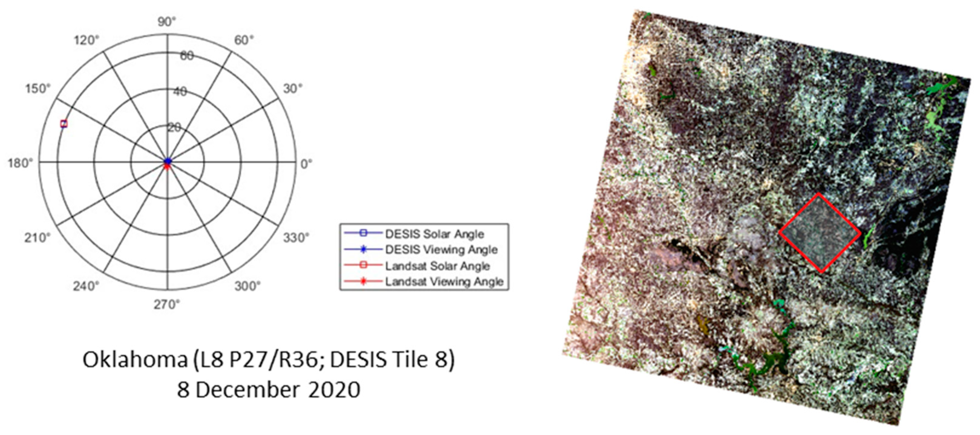
Figure 3 describes an example DESIS/L8 OLI image pair over Oklahoma (L8 P27/R36 and DESIS Tile 8). The figure includes a polar plot of the image pair’s solar (zenith and azimuth) and sensor viewing (zenith and azimuth) angles. It also shows how the footprints of each image lie on the Earth with respect to each other.

2.3. Processing Workflow

The near-coincident cross-calibration workflow contains six elements, as shown in

Table 5. Near-coincident Cross-Calibration Workflow Elements.

Element	Purpose	Comment
Spectral Synthesis	Simulates the multispectral instrument RSRs from the hyperspectral bandpasses	RSR knowledge is critical. SCR sampling and resolution must be commensurate with RSR spectral properties
Geometric Co-Registration	Improves registration between image pairs. Reduces scatter due to misalignment.	Direct georeferencing is not as accurate as image-to-image co-registration
Spatial Harmonization	Reduces scatter due to sampling and blurring (PSF) differences	Less critical over uniform areas. Reduces scatter in regression
Cloud and Cloud Shadow Screening	Removes outliers	Screening is critical
BRDF and Polarization Mitigation	Reduces biases between data sets	Scene and landcover can reduce impact. Near-SNOs reduce impact.
Regression/Outlier Removal	Estimates gain (and offset if required) and provides a fitting parameter uncertainty	For near-SNOs and remote sensing instruments with excellent dark frame correction, gain should be estimated with y = Bx model

. In this study, cloud/cloud shadow screening was accomplished as part of the identification of near-coincident DESIS/L8 image pairs by screening for only cloud-free imagery. Likewise, BRDF and polarization correction/mitigation was accomplished as part of the image pair selection process by only selecting image pairs acquired within 3.5 min of each other and with view zenith angles within 7°. The remaining workflow elements are discussed below.

2.4. Spectral Synthesis

Spectral synthesis is used to simulate a multispectral bandpass from multiple hyperspectral bands [23,24,25]. The spectral sampling and FWHM of the hyperspectral bands must be fine enough that when used to synthesize multispectral bands, they produce small TOA radiometric errors. CLARREO and TRUTHS, for example, have FWHM values that are ~2× the sampling frequency to reduce the effects of aliasing. Since spectral errors are mapped into radiometric errors, it is critical for the reference and client instruments’ RSRs to be well known.

For each spectral bandpass, spectral synthesis follows the model

$$S_T=S_H\beta$$

(1)

where $S_T$ are the relative spectral responses of the target multispectral instrument, $S_H$ are the hyperspectral RSRs used to simulate the target multispectral band passes and $\beta$ are the coefficients applied to each hyperspectral band to best fit any one multispectral bandpass using ordinary least squares. This spectral synthesis approach is area preserving, thus minimizing errors. In long-hand notation, for any one target multispectral band, the model can be expressed as

$$\left[\begin{array}{c}{S}_{T1}\\ S_{T2}\\ ⋮\\ S_{TN}\end{array}\right]=\left[\begin{array}{c}{S}_{H11}{ S}_{H21}\dots S_{HM1}\\ S_{H12}{ S}_{\mathrm{H}22}\dots S_{HM2}\\ ⋮ ⋮ ⋮ \\ S_{H1N}{ S}_{H2N}\dots S_{HMN}\end{array}\right]\left[\begin{array}{c}{\beta }_1\\ {\beta }_2\\ ⋮\\ {\beta }_M\end{array}\right]$$

(2)

where there are N specified locations along a particular target multispectral spectral response function and M hyperspectral bands. In this case, $S_{Ti}$, where i goes from 1 to N, are values of the relative spectral responses for a target (reference or client) multispectral band at different spectral locations. ${\beta }_{\mathrm{j}}$ is the array of coefficients applied to each hyperspectral band going from 1 to M hyperspectral bands. $S_{Hji}$, where j goes from 1 to M hyperspectral bands, and i goes from 1 to N spectral locations, are the M × N array of hyperspectral RSR values used in the simulation. In this formulation, each hyperspectral band has the opportunity of contributing to each target relative spectral response at each spectral location defining the target multispectral bandpass. The coefficients are calculated via an ordinary least squares solution:

$$\beta ={\left({S_H}^T{S}_H\right)}^{-1}{S_H}^T{S}_T$$

(3)

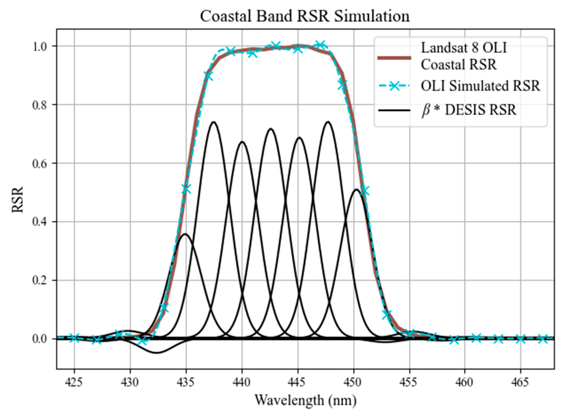
An example L8 OLI multispectral band (coastal aerosol) spectral response and the band synthesized using DESIS spectral responses are shown in Figure 4. The figure also shows the DESIS hyperspectral spectral responses scaled by $\beta$. Based on the DLR’s wavelength calibration and FWHM measurements [26], DESIS’ spectral bands are modeled as Gaussian spectral shapes.

Figure 5, Figure 6, Figure 7, Figure 8 and Figure 9 show the complete set of actual L8 bands and bands simulated with DESIS hyperspectral imagery using spectral synthesis.

Once spectral synthesis coefficients are derived, they are applied to the DESIS L1C radiance imagery to produce spectrally harmonized, simulated L8 multispectral images. The DESIS-provided quality layer identifies suspect pixels for each band. DESIS contains a manufacturing defect that affects a large number of pixels in the first seven spectral bands [21]. During spectral synthesis, these suspect pixels are not used.

After spectral synthesis is employed, simulated multispectral radiance data, $L_{TOA}$, is converted to TOA reflectance ${\rho }_{TOA}$ using a per-pixel solar zenith angle, ${\theta }_z$, the Earth–Sun distance, $d$, and a Landsat-derived exo-atmospheric solar irradiance ($ESUN$) value.

$${\rho }_{TOA}=\frac{\pi d^2{L}_{TOA}}{ESUN \mathrm{c}\mathrm{o}\mathrm{s} \left({\theta }_z\right)}$$

(4)

Landsat TOA reflectance is derived using the onboard diffuser calibration and does not directly employ $ESUN$.

2.5. Image Co-Registration

Image registration is the process of aligning images in the spatial domain by transforming the image’s given coordinates into a set of standard reference coordinates. This process is necessary to reduce the scatter in the regression analysis and to create a more accurate fit to the data.

Data provided by direct georeferencing can have errors ranging from 20 m to 1 km [27], depending on the satellite, which may not be sufficient for cross-calibration. When relying on internal satellite measurements alone, DESIS has a root mean square error (RMSE) of 298 m to 496 m in the across and along tracks, respectively [16]. When using ground control points (GCPs) or other reference points, this reduces to an RMSE of approximately 28 m [26].

A registration algorithm that increases the relative geometric accuracy between two images was developed to reduce direct georeferencing errors. In this algorithm, each pair of images—one being the L8 OLI reference and the other a DESIS spectrally synthesized multispectral image—are cropped to their intersection and a uniform, staggered grid of points are generated for chip matching. Image chips (64 × 64 pixels) around each point in the grid are generated for the simulated and reference datasets. The chips are then “matched” using a singular value decomposition phase correlation method (SVD PCM) from [28]. The SVD PCM uses the singular value decomposition of the normalized cross power spectrum between two image chips to estimate the shifts between them. Once all the points have been matched between the two datasets, an affine transform is estimated using ordinary least squares. Images are warped using a cubic convolution interpolation algorithm [29]. Fill values are tracked in the interpolation process. The chip generation and matching process is repeated for each new warped image for n iterations to increase the final registration’s accuracy. All affine transforms generated in the iterative process are combined to form a final transform that warps the initial simulated dataset. The entire registration process is completed with a single interpolation step introduced to the original dataset and is performed per simulated band.

2.6. Spatial Harmonization

Spatial resolution determines the smallest feature that can be resolved in an image, and is controlled by pixel size (GSD), image sharpness (or blur), and image noise [30]. In most cases, the hyperspectral imager’s spatial resolution will not match the reference or client instrument’s spatial resolution. Harmonizing or matching the SCR’s spatial resolution removes errors that are introduced in scenes with high spatial content. In this study, since the GSDs of L8 and DESIS are 30 m, spatial harmonization is initially accomplished by blurring one system to match the other. To evaluate the effect of GSD on SCR performance, GSD parametric sweeps were conducted. In these parametric sweep cases, downsampling, to match GSD, is also performed. Since L8 and DESIS provide extremely high SNR imagery [7,11], image noise was not taken into account during spatial harmonization.

Landsat 30 m GSD imagery is sharper than DESIS 30 m GSD imagery. For L8 L1R imagery, the modulation transfer function (MTF)@Nyquist is ~0.4, and slightly lower after rectification. DESIS has an MTF@Nyquist of ~0.2, which indicates less aliasing than Landsat. After co-registration, the L8 OLI reference and DESIS-simulated multispectral images are segmented into a grid of corresponding 128 × 128 pixel chips for which the discrete Fourier transform (DFT) amplitude is calculated. Using these amplitude spectra, we calculate the median value of the ratio at each spatial frequency to produce a transfer function that is fitted to a bivariate Gaussian function. The resulting transfer function is then applied to the Landsat imagery in order to make it more spatially similar to the DESIS-simulated multispectral imagery.

2.7. Regression

The image regressions performed in this assessment are based on gain only, and rely on the hyperspectral and reference instruments’ signals being linear and having minimal offsets after dark frame corrections. The highly calibrated L8 OLI operates detectors at −63 °C to achieve low noise and drift [31]. For DESIS, the FPA is temperature stabilized and a dark frame is determined by taking dark frames before and after scanning [26]. The dark signal is subtracted from the illuminated signal, which is scaled to radiance using a gain.

Both L8 OLI (reference) and DESIS (hyperspectral surrogate SCR) have Level 1 ($L1$) products in the form:

$$L1=G({DN}_{Lin}-{DN}_{Dark})$$

(5)

where $L1$ is TOA reflectance or radiance, ${DN}_{Lin}$ is the linearized digital count, ${DN}_{Dark}$ is the dark frame correction, and $G$ is a gain factor. Other parameters that could cause deviations from linearity (e.g., stray light in the case of Landsat) have been minimized for Landsat [32].

DESIS’ and L8 OLI’s well-known dark frames, and minimal offsets after dark frame subtraction, enable the cross-calibration in this study to be represented by the following linear equation:

$$y=Bx$$

(6)

The slope (gain), $B$, for $x_i$, $y_i$ (L8, DESIS-simulated L8) pixel pairs is calculated using least squares with ${\sigma }_i$ being the standard deviation of $y_i.$ Pixel pairs were selected as the center pixel value of each 3 × 3 pixel patch that met the COV < 0.05 threshold.

$$B=\frac{\sum \frac{x_i{y}_i}{{\sigma }_i^2}}{\sum \frac{x_i^2}{{\sigma }_i^2}}$$

(7)

Using this formulation, an analytical uncertainty can be calculated as follows:

$${\sigma }_B=\frac{1}{\sqrt{\sum \frac{x_i^2}{{\sigma }_i^2}}}$$

(8)

This cross-calibration approach fits data pairs (in this case L8 and DESIS-simulated L8) with a linear model, which allows one to analyze the residuals for data anomalies.

A simple bootstrap method described in [33] was employed to provide other estimate of fit parameter uncertainties. The method uses the original dataset $D_0$ of size $N$ to draw some number, $n$, of random samples, $D_1,D_2,D_3,\dots D_n$ with replacement (each also of size $N$). Each random sample is a unique set of points due to random replacement. The fit parameters for each sample, $B_1, B_2, B_3, \dots B_n$ are estimated, which center around $B_0$, with the standard deviation of the samples used as an estimate of the uncertainty in $B_0$.

Even as VNIR-system FPAs carry temperature sensors and their behavior is known as a function of temperature, i.e., the dark frame is typically well known and well behaved, in cases where an SCR is transferring calibration back to a client VNIR instrument, a linear regression that includes an offset, in addition to gain, may need to be considered.

2.8. Outlier Removal

After the spectrally and spatially harmonized data from DESIS and L8 OLI are paired and co-registered, outliers, potentially due to misregistration and point spread function (PSF) matching errors, or as a result of resampling image pairs to each other, are avoided by applying a coefficient of variation (COV) threshold to blocks of pixels. The COV is calculated using 3 × 3 pixel regions. Regions with a COV less than 0.05 in both L8 OLI and DESIS-simulated L8 OLI data are identified as uniform regions and used for the assessment. These pixels are plotted against each other and regressed using an equally weighted ordinary least squares method to determine the quality of the fit, measured by its parameters, uncertainties, and coefficient of determination (R²).

3. Results

3.1. Cross-Calibration

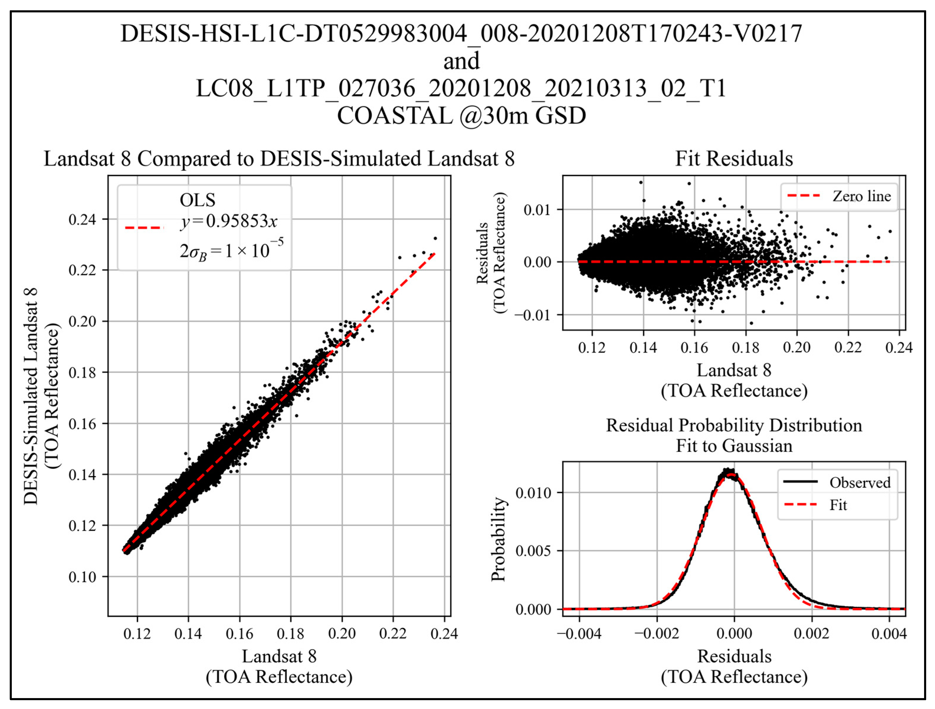
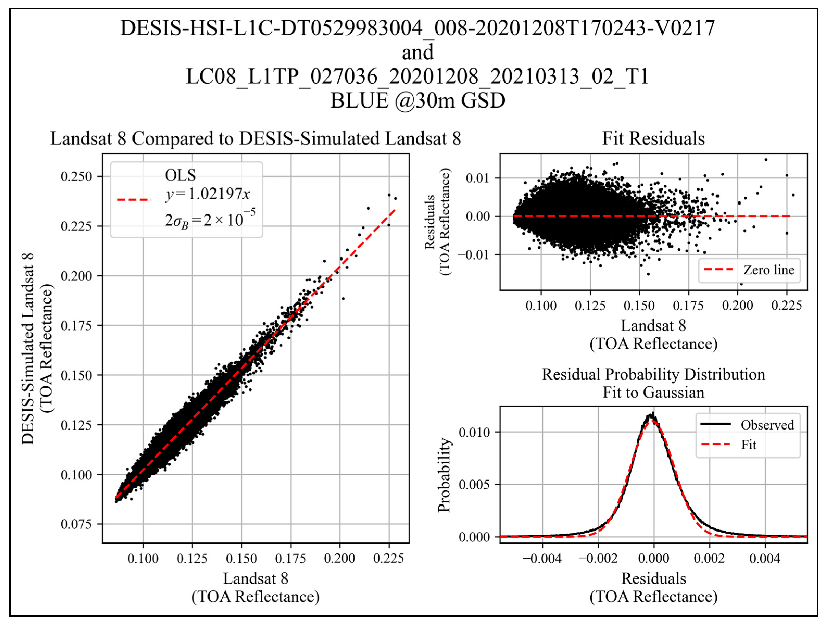
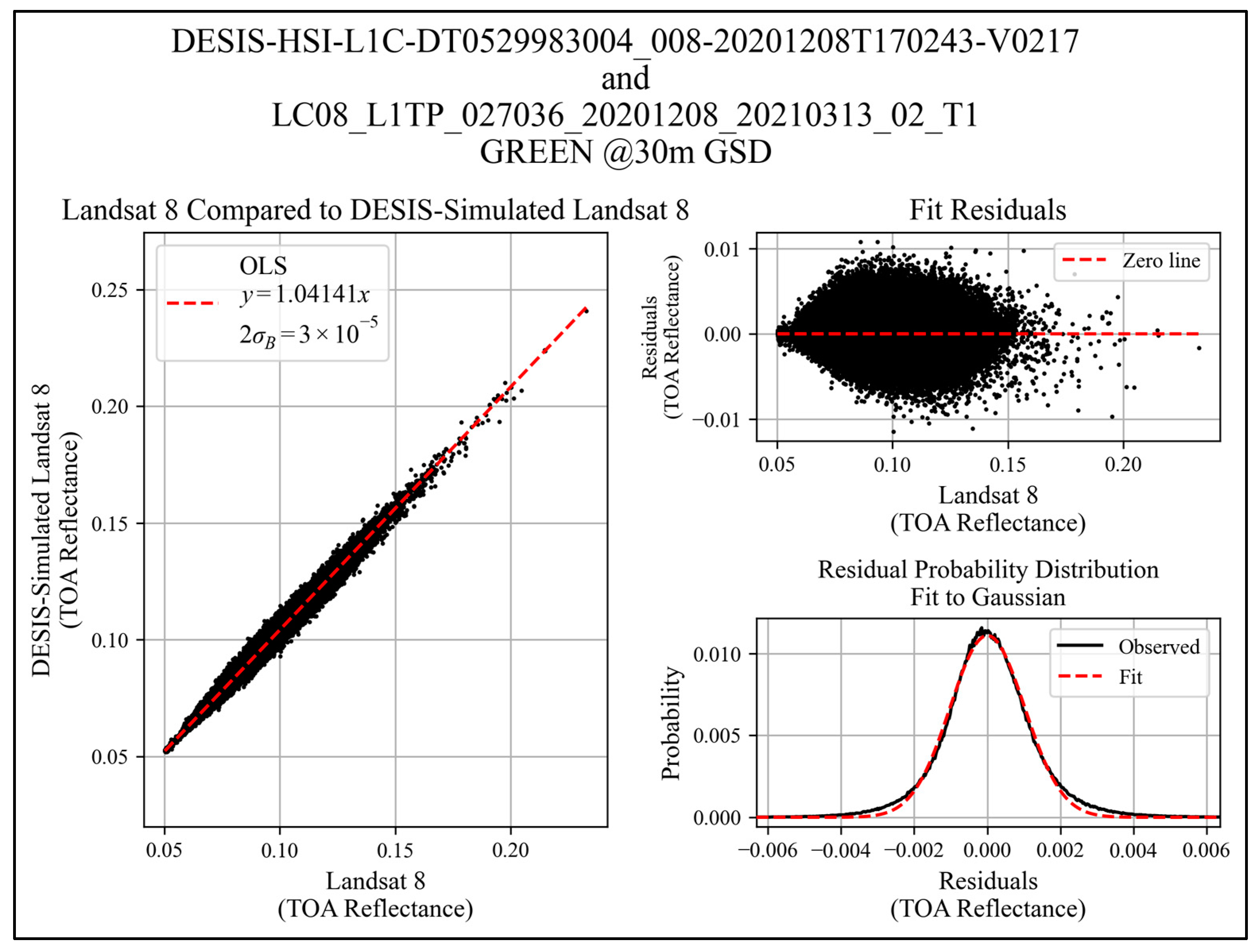
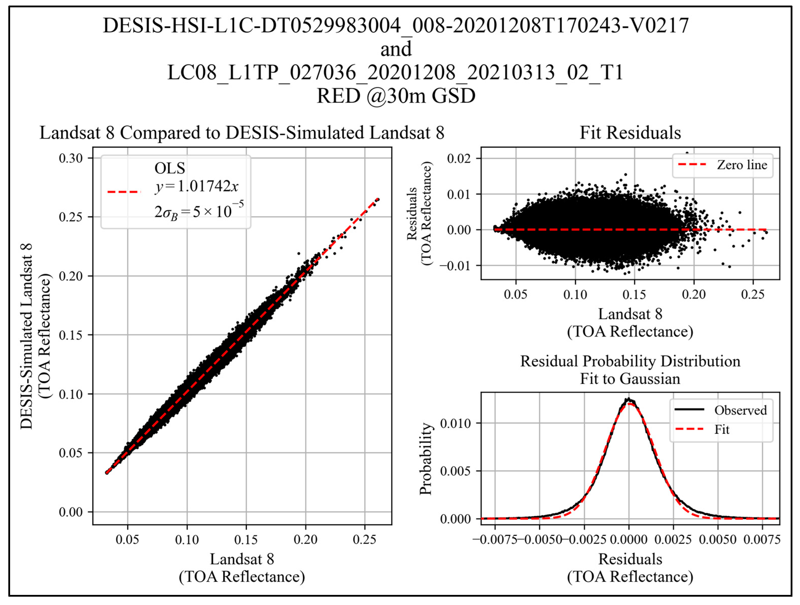
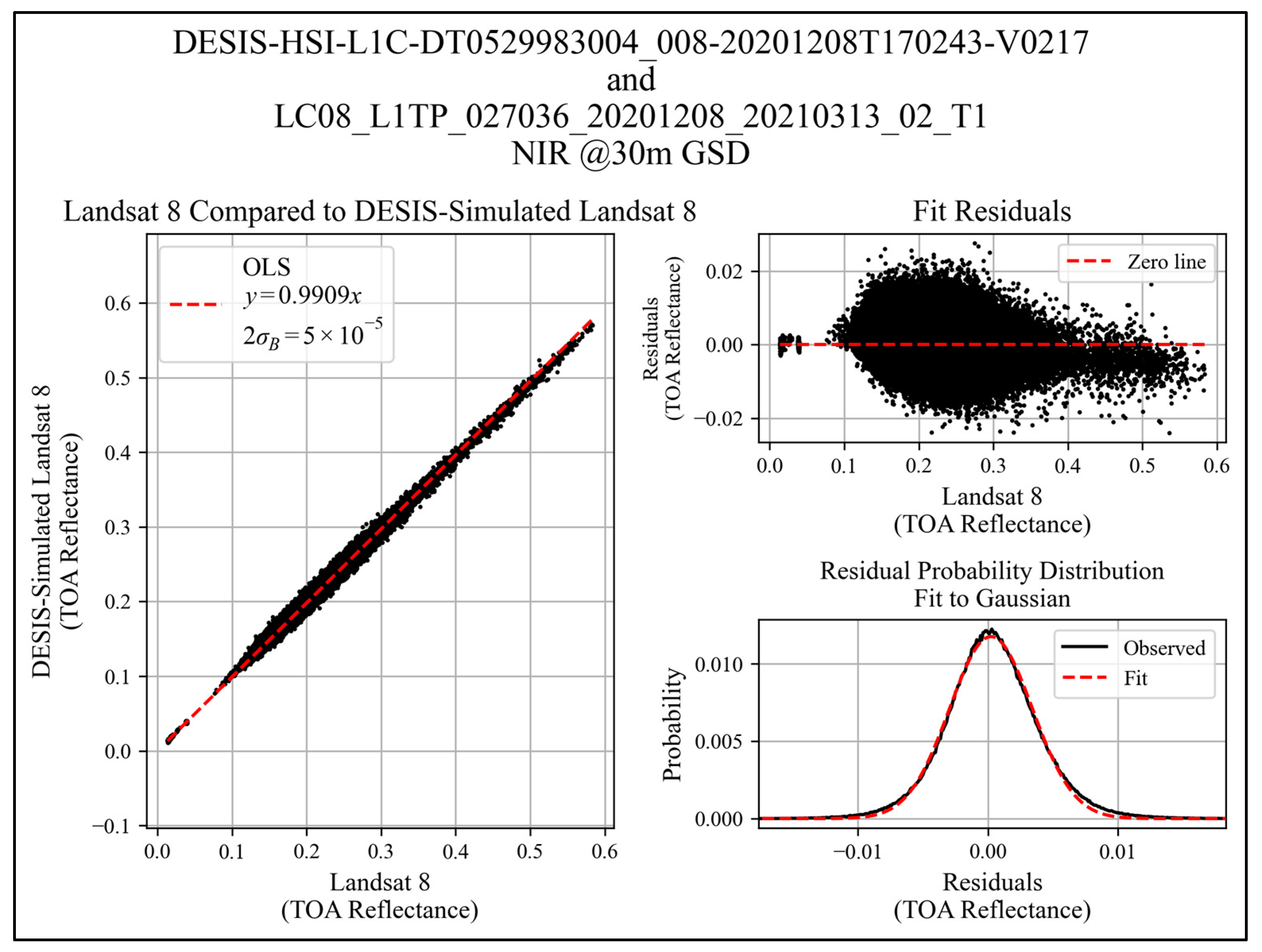
Example regression plots that transfer calibration from a reference to an SCR, and their associated residuals for the coastal aerosol, blue, green, red, and NIR bands are shown in Figure 10, Figure 11, Figure 12, Figure 13 and Figure 14 for the Oklahoma image pair discussed above (L8 P27/R36; DESIS Tile 8, baseline 30 m GSD). The example shown is a highly vegetative site, so apart from the NIR band, the TOA reflectances cover a narrow range of values. These figures give uncertainties at the 95% confidence interval (2σ). Fit residuals show near-ideal normal distributions with peak-to-peak ranges less than 0.02 in all cases consistent with the COV threshold. Residual distributions were fit to a Gaussian function and qualitatively show high quality fits. Additionally, a Kolmogorov–Smirnov normality test was performed and confirmed residual distributions likely belong to the fit Gaussian distributions.

Table 6. Fitted Gain ($B$) with Uncertainty (${\sigma }_B)$ for Each Cross-Calibration Test Set.

Location	L8 Path/Row	DESIS Tile	Date	Coastal Aerosol		Blue		Green		Red		NIR
				$\mathit{B}$	$2{\mathit{\sigma }}_{\mathit{B}}$	$\mathit{B}$	${2\mathit{\sigma }}_{\mathit{B}}$	$\mathit{B}$	$2{\mathit{\sigma }}_{\mathit{B}}$	$\mathit{B}$	$2{\mathit{\sigma }}_{\mathit{B}}$	$\mathit{B}$	$2{\mathit{\sigma }}_{\mathit{B}}$
Corona, NM	033/036	1	28 August 2020	0.946	3 × 10−5	1.006	3 × 10−5	1.025	3 × 10−5	1.001	3 × 10−5	0.975	2 × 10−5
Oklahoma	027/037	2	8 December 2020	0.914	2 × 10−5	0.967	3 × 10−5	0.990	4 × 10−5	0.970	6 × 10−5	0.957	4 × 10−5
Oklahoma	027/036	8	8 December 2020	0.959	1 × 10−5	1.022	2 × 10−5	1.041	3 × 10−5	1.017	5 × 10−5	0.991	5 × 10−5
Oklahoma	027/035	11	8 December 2020	0.970	2 × 10−5	1.032	2 × 10−5	1.055	4 × 10−5	1.029	7 × 10−5	0.997	6 × 10−5
Paraguay	225/077	3	9 March 2021	0.918	4 × 10−5	0.980	4 × 10−5	1.001	4 × 10−5	0.974	4 × 10−5	0.966	3 × 10−5
Paraguay	225/078	7	9 March 2021	0.972	3 × 10−5	1.050	4 × 10−5	1.073	5 × 10−5	1.050	6 × 10−5	1.016	5 × 10−5
Egypt 1	178/042	11	29 December 2021	1.014	1 × 10−5	1.059	1 × 10−5	1.053	1 × 10−5	1.030	1 × 10−5	1.008	1 × 10−5
Egypt 1	178/043	14	29 December 2021	1.028	1 × 10−5	1.074	1 × 10−5	1.062	2 × 10−5	1.033	2 × 10−5	1.010	2 × 10−5
Mauritania 2	201/045	33	30 December 2021	0.998	2 × 10−5	1.043	2 × 10−5	1.048	1 × 10−5	1.027	1 × 10−5	1.007	1 × 10−5
Mauritania 2	201/046	37	30 December 2021	1.030	1 × 10−5	1.076	2 × 10−5	1.064	2 × 10−5	1.037	1 × 10−5	1.014	1 × 10−5
Snow Mt., CA	044/032	7	9 April 2022	0.933	3 × 10−5	0.985	3 × 10−5	1.009	5 × 10−5	0.981	1 × 10−4	0.954	5 × 10−5
			Mean	0.971	2 × 10−5	1.027	2 × 10−5	1.038	3 × 10−5	1.014	4 × 10−5	0.990	3 × 10−5
			Median	0.970	2 × 10−5	1.032	2 × 10−5	1.048	3 × 10−5	1.027	4 × 10−5	0.997	3 × 10−5
			Std. Dev.	0.042	1 × 10−5	0.038	1 × 10−5	0.028	1 × 10−5	0.028	3 × 10−5	0.023	2 × 10−5
			Min	0.914	1 × 10−5	0.967	1 × 10−5	0.990	1 × 10−5	0.970	1 × 10−5	0.954	1 × 10−5
			Max	1.030	4 × 10−5	1.076	4 × 10−5	1.073	5 × 10−5	1.050	1 × 10−4	1.016	6 × 10−5

summarizes the fitted gain and uncertainty in fitted gain for each band (coastal aerosol, blue, green, red, and NIR) for all eleven sites selected for this study. The estimated uncertainties are extremely small due to the large sample size. In most cases, the number of points used in the regression approaches 10⁶ points. Errors in gain uncertainty do not include any error in the abscissa, meaning the L8 TOA reflectance is, in this analysis, considered perfect. Standard statistics (i.e., mean, median, standard deviation, minimum, and maximum values) are also shown in the table.

While near-SNOs were used, there is a few percent scatter in the slopes at each site and date, likely caused by small BRDF effects and instrument drift over the nearly two-year period this imagery was drawn from. Land cover at the different sites is diverse and not necessarily Lambertian. Small instrument drift requires DLR to periodically update the DESIS radiometric calibration, and these adjustments are discrete. To achieve transfer calibrations within ~1%, the SCR’s drift will need to be small and the slope (gain) scatter will need to be reduced by averaging over many sites and selecting sites with known and low BRDF land covers.

3.2. Performance Trades

3.2.1. Ground Sample Distance (GSD) Effect on Cross-Calibration Results

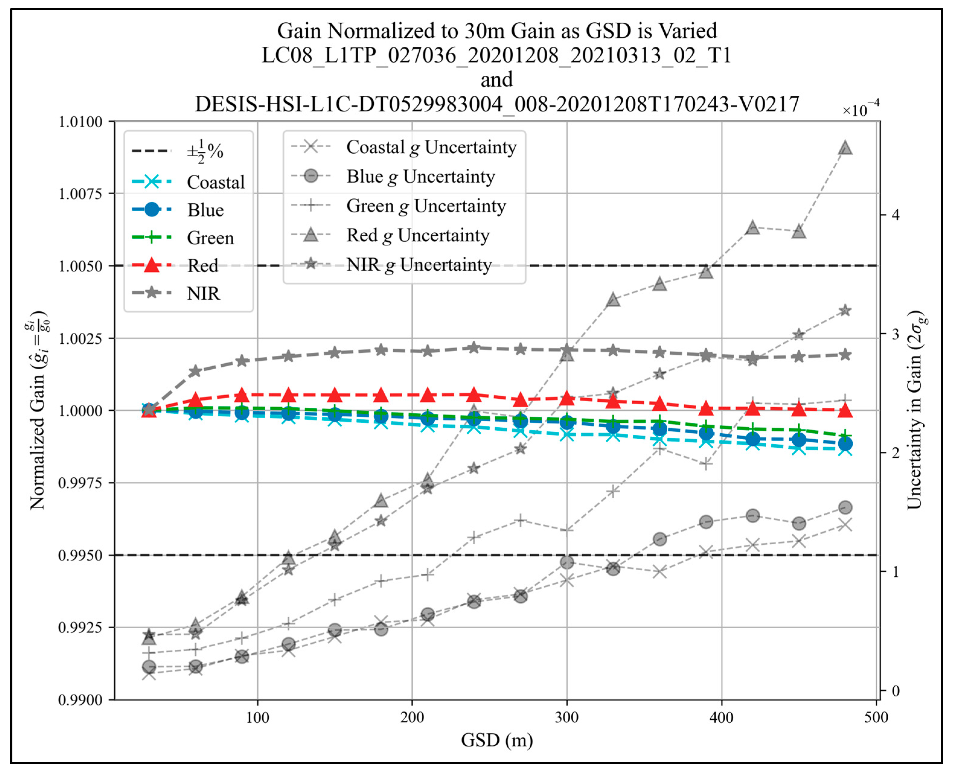
For the purposes of evaluating the effect of GSD on cross-calibration results (gain), L8 and DESIS-simulated L8 image pairs for potential SCR GSDs ranging from 30 m to 480 m, in increments of 30 m, were generated. A Gaussian filter with a FWHM equal to 1.64 times the GSD was used to minimize aliasing in each successive GSD. After the images were downsampled to each desired resolution, the COV threshold filter discussed above (COV < 0.05) was applied. Figure 15 shows the influence of GSD for the Oklahoma cross-calibration site (L8 P27/R36 and DESIS Tile 8) discussed above. Normalized gain, or the gain achieved at a particular GSD with respect to the gain achieved at a 30 m GSD is plotted. The normalized gain dependence for this case is less than 0.25% for each spectral band over the entire GSD sweep. The figure also shows the uncertainty (2σ) in gain that grows with the GSD, which is due to fewer samples (pixels) at larger GSD values. The largest gain uncertainty for this cross-calibration image pair is in the red band and ~0.05% for an SCR GSD of 480 m. In addition, there is a small rise in the NIR normalized gain between the 30 and 60 m GSD due to small spatial harmonization errors at these GSDs.

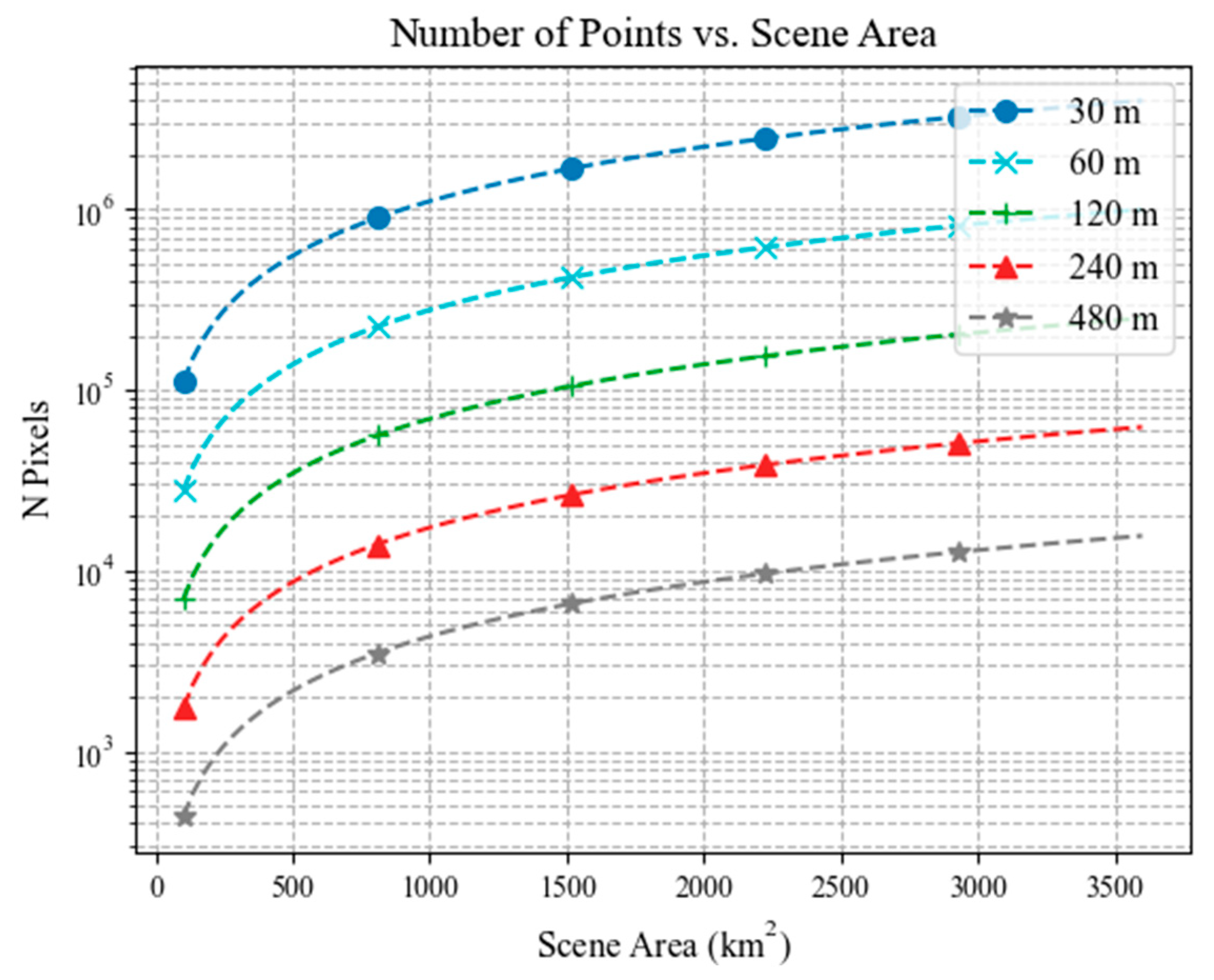
3.2.2. Effect of the Number of Independent Spatial Samples on Cross-Calibration Results

The number of spatial samples (pixels) depends not only on the GSD of an SCR, but also on the extent of the overlapping area between an SCR image and client (or reference) instrument image. Figure 16 shows that except for very small SCR-client (or SCR-reference) image acquisition overlap areas <~250 km² and large SCR GSDs, near 480 m, the number of spatial samples available for a cross-calibration will exceed 1000.

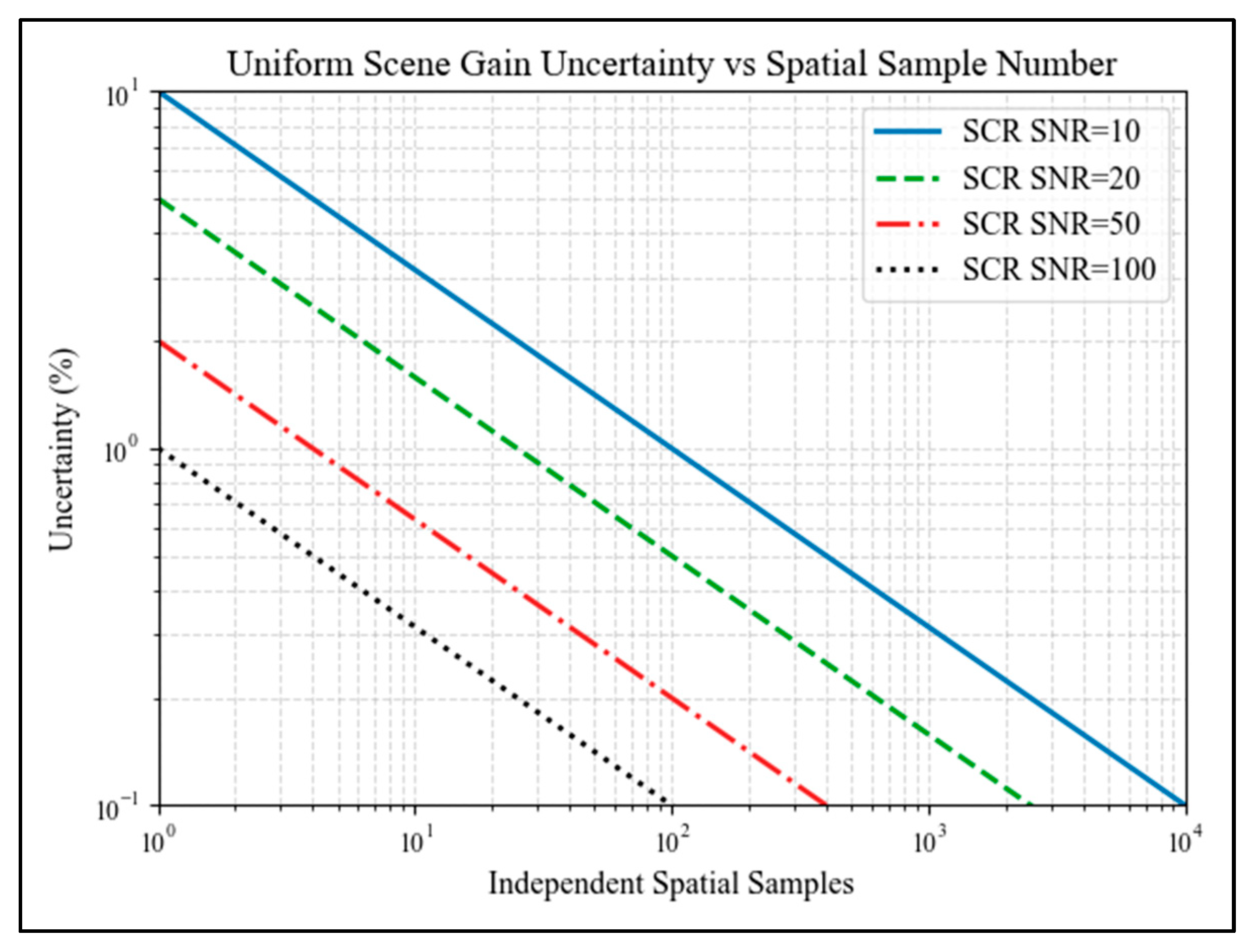
Assuming all noise sources are uncorrelated, gain uncertainty is approximately inversely proportional to the square root of the number of independent spatial samples. Knowing the SNR of a single spatial sample after spectral synthesis ($SN{R}_{SCR})$, one can estimate how many samples ($N_{samples})$ are required to achieve the desired uncertainty ($Un{c}_{Gain}$).

$$N_{samples}={\left(\frac{1}{Un{c}_{Gain} SN{R}_{SCR}}\right)}^2$$

(9)

In this construction, the uncertainty $Un{c}_{Gain}$ could be due to the instrument (as instrument noise) or the scene (as small scene nonuniformities). The $SN{R}_{SCR}$ value includes all noise sources and not just instrument noise. It also assumes that the noise associated with the reference instrument (i.e., truth), as discussed above, is negligible. Based on this relationship, 10,000, 2500, 400, and 100 spatial samples will be required to achieve 0.1% gain uncertainty for single-pixel $SN{R}_{SCR}$ values of 10, 20, 50, and 100, respectively. By extension, 100, 25, 4, and 1 spatial samples are necessary to achieve a 1% gain uncertainty.

Figure 17 further illustrates the relationship between slope (gain) uncertainty and the number of independent spatial samples in a uniform scene. It shows that the effects of the SNR can be reduced to negligible levels by incorporating many samples into the cross-calibration.

3.2.3. Misregistration Effect on Cross-Calibration Results

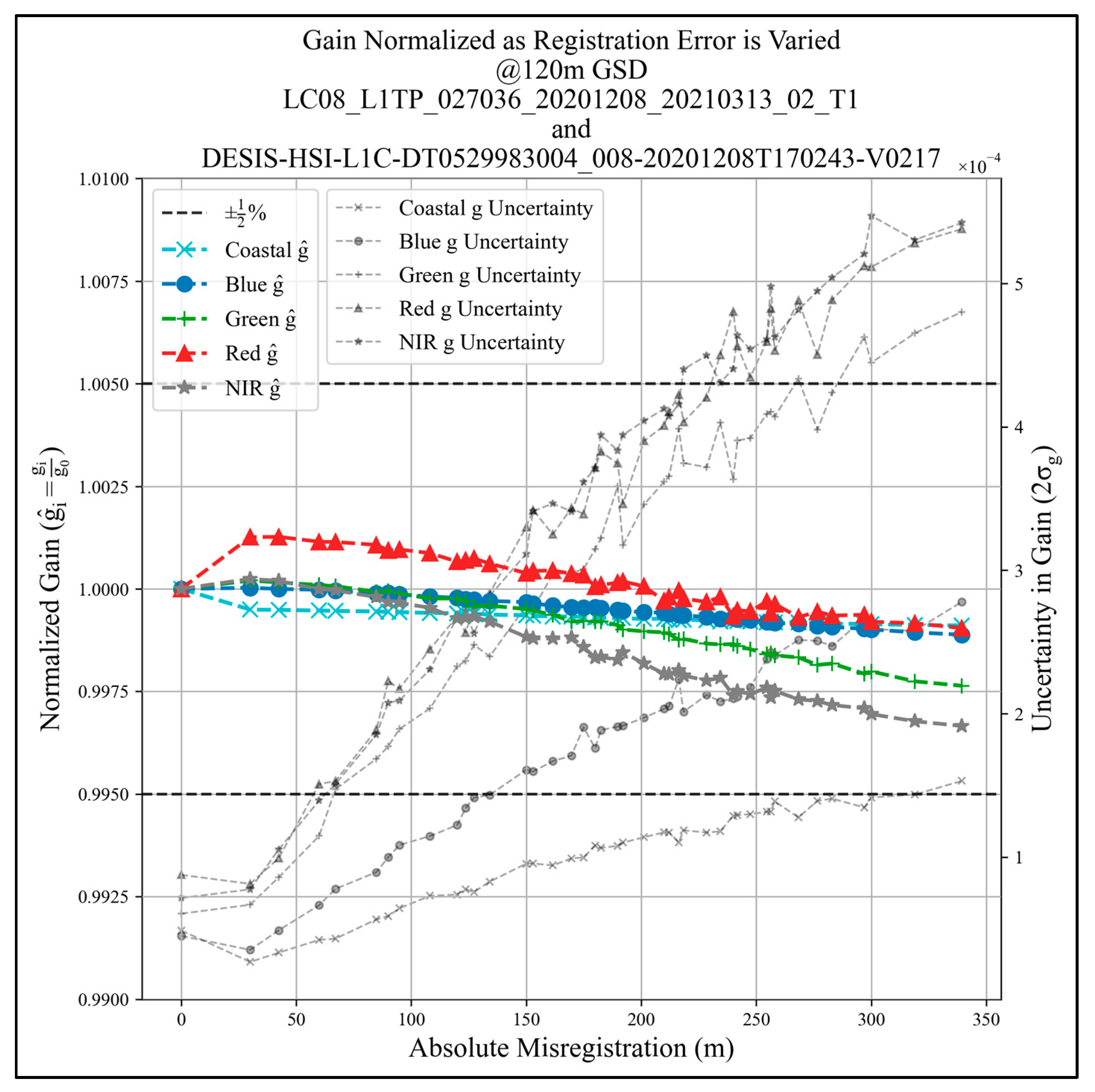
To evaluate the effect of misregistration on cross-calibration results (gain), L8 and DESIS-simulated L8 image pairs were parametrically misregistered in both the row and column direction. The image pairs that were used had a 120 m GSD and were initially co-registered. Missregistrations varied up to 240 m (2 pixels) in both the row and column direction for a total misregistration of ~339 m. Figure 18 shows the influence of misregistration for the same Oklahoma cross-calibration site (L8 P27/R36 and DESIS Tile 8) discussed above. In the misregistration range investigated, normalized gain, or the gain achieved at a particular misregistration with respect to the gain achieved using co-registered image pairs is less than 0.25%. While the uncertainty in gain (2σ) increases with increasing misregistration, it does not exceed 0.06%.

3.2.4. PSF Effect on Cross-Calibration Results

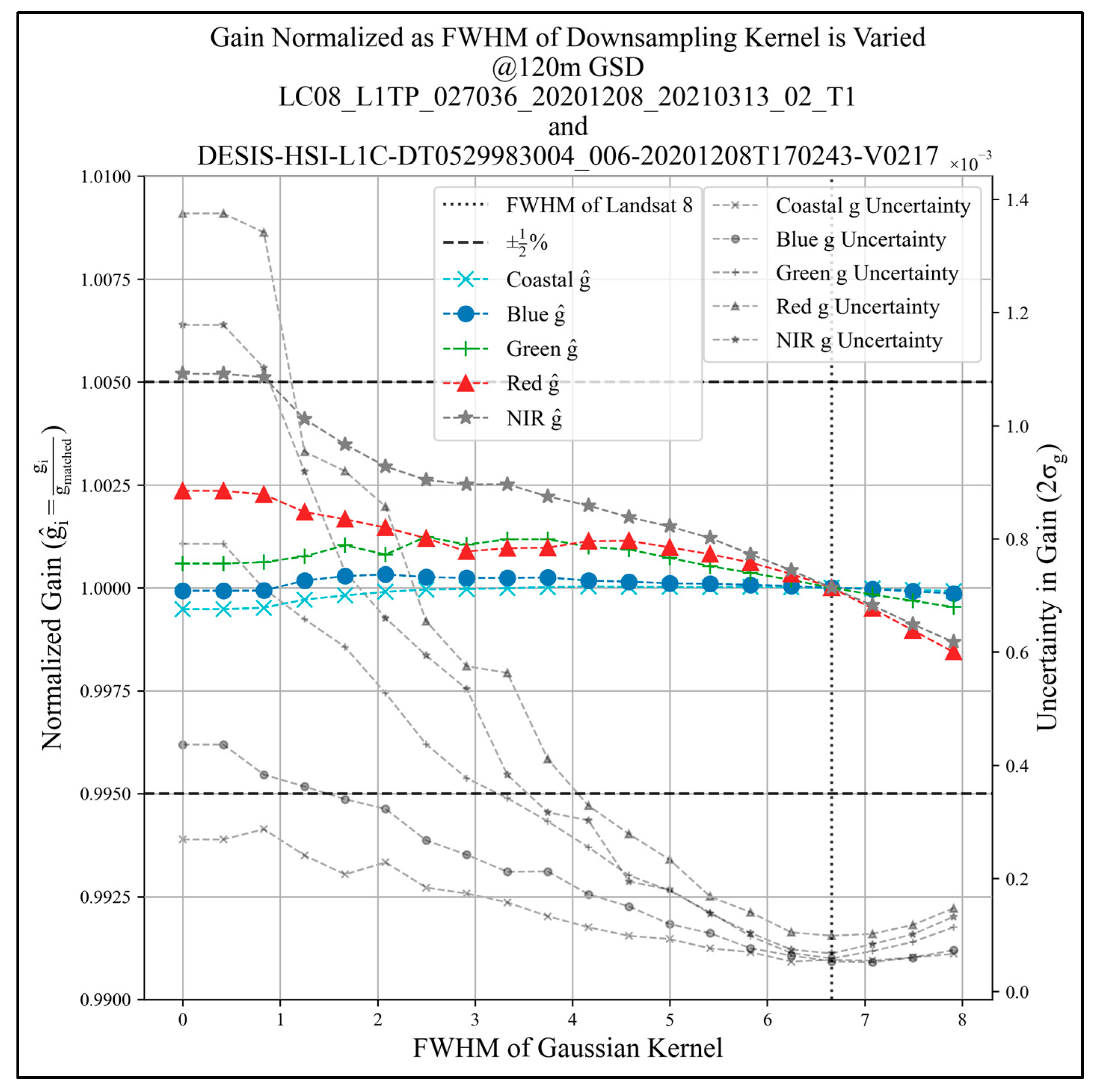
To evaluate the effect of PSF (image blur) on cross-calibration results (gain), a Gaussian kernel with a varying FWHM was applied to both the L8 and DESIS-simulated L8 image pairs. The image pairs that were used had a 120 m GSD. A baseline image blur was established by applying a Gaussian kernel with a FWHM equal to that of Landsat 8 to both images. FWHM values ranged from 0 to a maximum of 8. Figure 19 shows the influence of image blur for the same Oklahoma cross-calibration site (L8 P27/R36 and DESIS Tile 8) discussed above. In the range investigated, normalized gain, or the gain achieved at a particular image blur with respect to the gain achieved using the baseline image blur, is <0.25%. While uncertainty in gain (2σ) increases with image sharpness, it does not exceed 0.14%.

4. Discussion

Eleven near-coincident image pairs from L8 OLI and DESIS, acting as an SCR surrogate, were used to perform SCR-reference instrument cross-calibrations over various land covers. DESIS imagery was spectrally and spatially harmonized to match L8 OLI and care was given to minimize differences in the BRDF and scene-induced polarization. Near-SNO conditions also reduced any differences in atmospheric conditions between the two image acquisitions. The mean uncertainty in gain (2σ) was on the order of 1.0 × 10⁻⁵ independent of band, predominately due to the large number (~10⁶) of independent samples used in the regression.

Parametric trades with varying GSD showed only minor influences (<0.25%) in resulting gain and, while moderate, showed increased uncertainty in gain with an increased GSD due to a smaller number of spatial samples. Uncertainty in gain increased approximately ten-fold to a maximum of nearly 5 × 10⁻⁴ in the red band for one scene.

Increasing GSD and blur also reduces the dynamic range of the scene used for cross-calibration due to pixel mixing and fewer remaining pure pixels, which, if taken too far will limit linearity evaluations in addition to further increasing gain uncertainty.

Since the uncertainty in gain is inversely proportional to both the square root of the number of independent samples and the SNR of the calibration (considering all noise sources, instrument, and scene nonuniformity), an SCR with a 10× lower SNR could produce the same gain uncertainty as a “baseline” SCR if 100× more independent samples were used when developing the calibration (gain).

Other factors that influence gain uncertainty and quality of fit are misregistration between image pairs, and different image PSFs (blur).

4.1. PSF Mismatch and Geometric Misregistration Impact on Quality of Fit

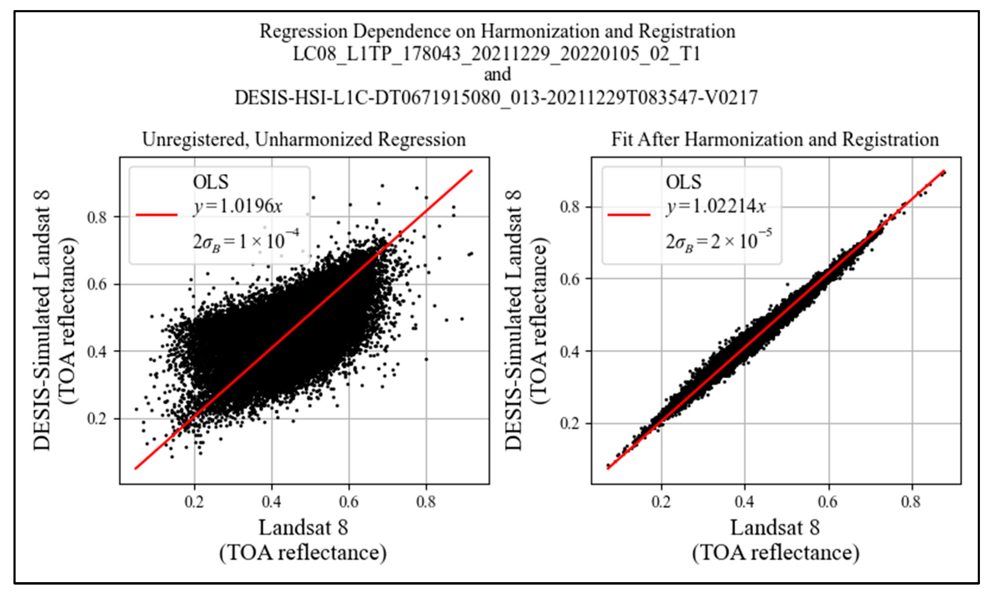
Both misregistration between image pairs and different levels of PSF (blur) between image pairs introduce noise and affect the quality of the regression. Figure 20 compares two DESIS-surrogate SCR cross-calibrations with L8 OLI. The cross-calibration between sensors on the left plot include a single pixel offset introduced in both the row and column directions. Differences in PSF were not accounted for, i.e., they were not harmonized. The MTF@Nyquist is ~0.4 for L8 L1R products and the (MTF)@Nyquist is ~0.2 for DESIS. The plot on the right shows imagery that is both spatially registered and harmonized (matched GSD and PSF). In this comparison example, the gain is almost identical (1.0196 vs. 1.0221), but the uncertainty in gain, while still small, differs by an order of magnitude. This indicates that, while statistically the same gain is achieved when working with PSF-matched image pairs that are registered as with not, a much higher quality regression fit is achievable when taking care to co-register the image pairs and match PSF.

4.2. Cloud Detection

The limitations in current cloud detection techniques necessitate the continued exploration of alternative cloud screening methods. This study relied on manual DESIS cloud screening, and Landsat cirrus bands to detect clouds. Also, detecting clouds can be difficult over bright, uniform targets (e.g., deserts and snow), often used for calibration. Advancing methods to mask/remove clouds that involve a baseline image and change detection or deep learning may be useful in the future. Clouds that shift between image pairs causing ground-pixels to be compared to cloud-pixels, however, show up as outliers in the regression.

4.3. Cross-Calibration Linear Regression Advantages

The linear regression technique used to estimate gain described in this paper provides an alternative to using only uniform scenes, such as RadCalNet or PIC sites. Limiting candidate scenes to extremely uniform areas significantly reduces the number of usable spatial samples and cross-calibration opportunities.

If a single scene or ensemble of image pairs cover the dynamic range of the sensor, regression allows the user to interrogate linearity not detected with traditional ground-based vicarious calibration. In the case of DESIS and L8 OLI, the residuals follow normal distributions and correlate with the selected COV threshold, which offers a simple way to remove outliers. The SNR of the calibration, which includes instrument noise and scene non-uniformities, can be small (<10 for Nsamples > 100) if there are enough spatial samples used in the regression, enabling the SCR to be used at the poles and in other low-light conditions. Even at coarse resolution (~500 m), cloud-free imagery from a moderately-sized SCR (<100 km swath) will have thousands of x, y pairs with uncorrelated noise.

4.4. Impact of Cross-Calibration Linear Regression Implementation on Instrument Design

A simple optical design, and one that is not necessarily diffraction limited, should not be excluded since the SCR’s calibration weakly depends on the GSD, PSF, and SNR. Most hyperspectral sensors need high SNRs, pushing the optical system’s speed. Smaller f-numbers mean larger, more complex optics, increased mass and volume, and more challenging optical alignment. Decreasing the f-number by a factor of two will decrease the aperture by a factor of two. Also, increasing the GSD reduces the focal length and the aperture diameter for a fixed f-number.

Table 7. Telescope Aperture Diameters as a function of GSD and f-number for a 600 km Orbital Altitude and 24 µm Slit.

GSD (m)	Telescope Aperture Diameter (mm)
	F/3	F/4	F/5	F/6
30	160	120	96	80
60	80	60	48	40
120	40	30	24	20
240	20	15	12	10
480	10	7.5	6	5

lists telescope aperture diameters for a 600 km orbital altitude with a 24 µm slit, comparable to DESIS, for various GSDs and f-numbers. For example, a DESIS-class system with a 30 m GSD operating at F/3 has an aperture diameter of ~160 mm. An SCR with a 120 m GSD and F/6 optics, half that of DESIS, would require only a 20 mm aperture. At this GSD, larger RadCalNet sites such as Railroad Valley NV can still be used for vicarious calibrations and the instrument could fit on a CubeSat.

5. Conclusions

This study shows that a DESIS-surrogate SCR could successfully be used to transfer calibration from a reference instrument such as L8 OLI. The study also shows that an SCR’s ability to determine the gain from cross-calibration is relatively insensitive to the SCR’s GSD or SNR. A large GSD, on the order of 480 m, could enable less expensive SCRs and possibly SCR constellations, since the mass and volume of individual instruments could be significantly reduced, even when compared with a 30 m GSD instrument. Constellations are desirable because they could significantly increase the number of near-SNOs. The downside of using a coarse resolution system is that it will limit the use of RadCalNet and other vicarious calibration techniques that require smaller pixels.

Cross-calibration, which employs the linear regression of scenes with varying land cover, allows many more pixels to be used in the analysis than traditional vicarious calibrations that use small uniform regions. In addition to providing insight into linearity, this type of cross-calibration increases the number of independent samples, which further drives down uncertainty. This study also shows that image co-registration and PSF matching reduce the scatter seen in the linear regression.

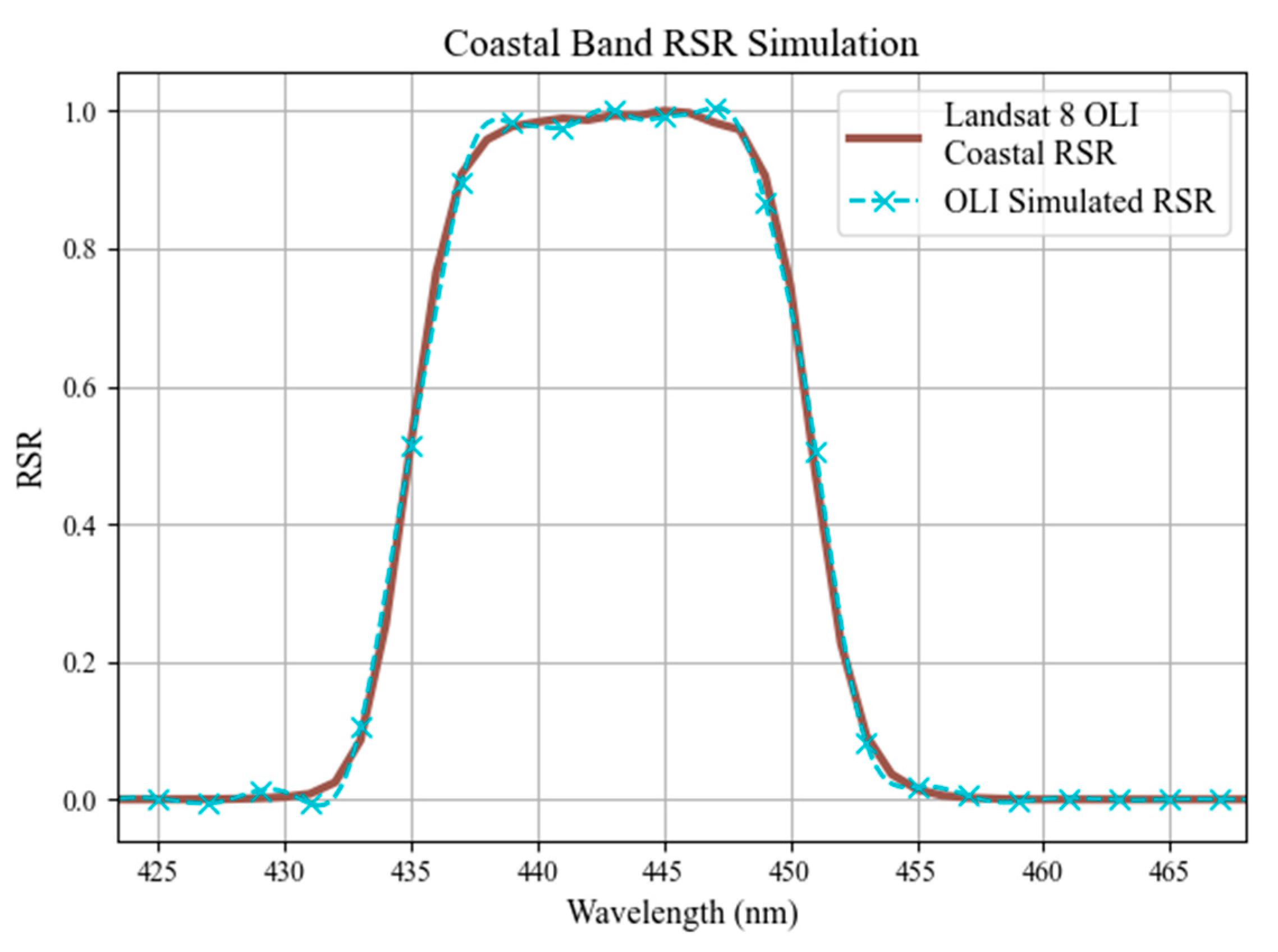
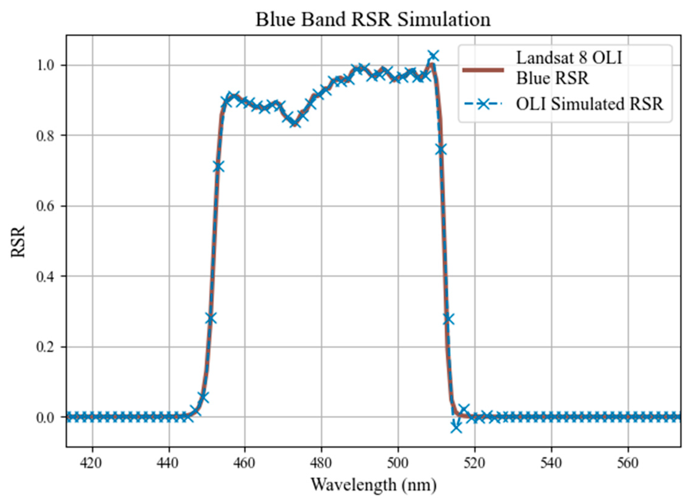
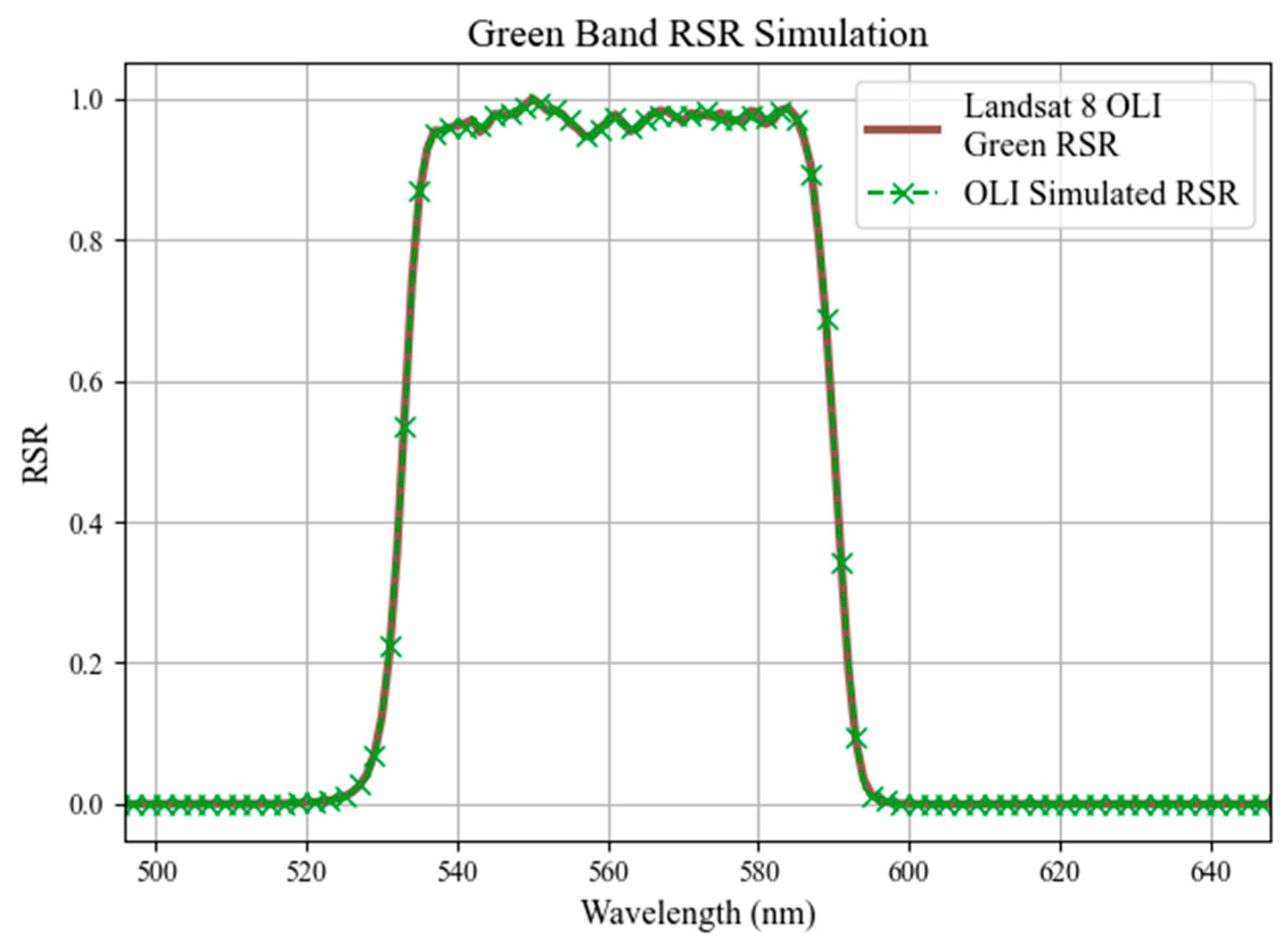
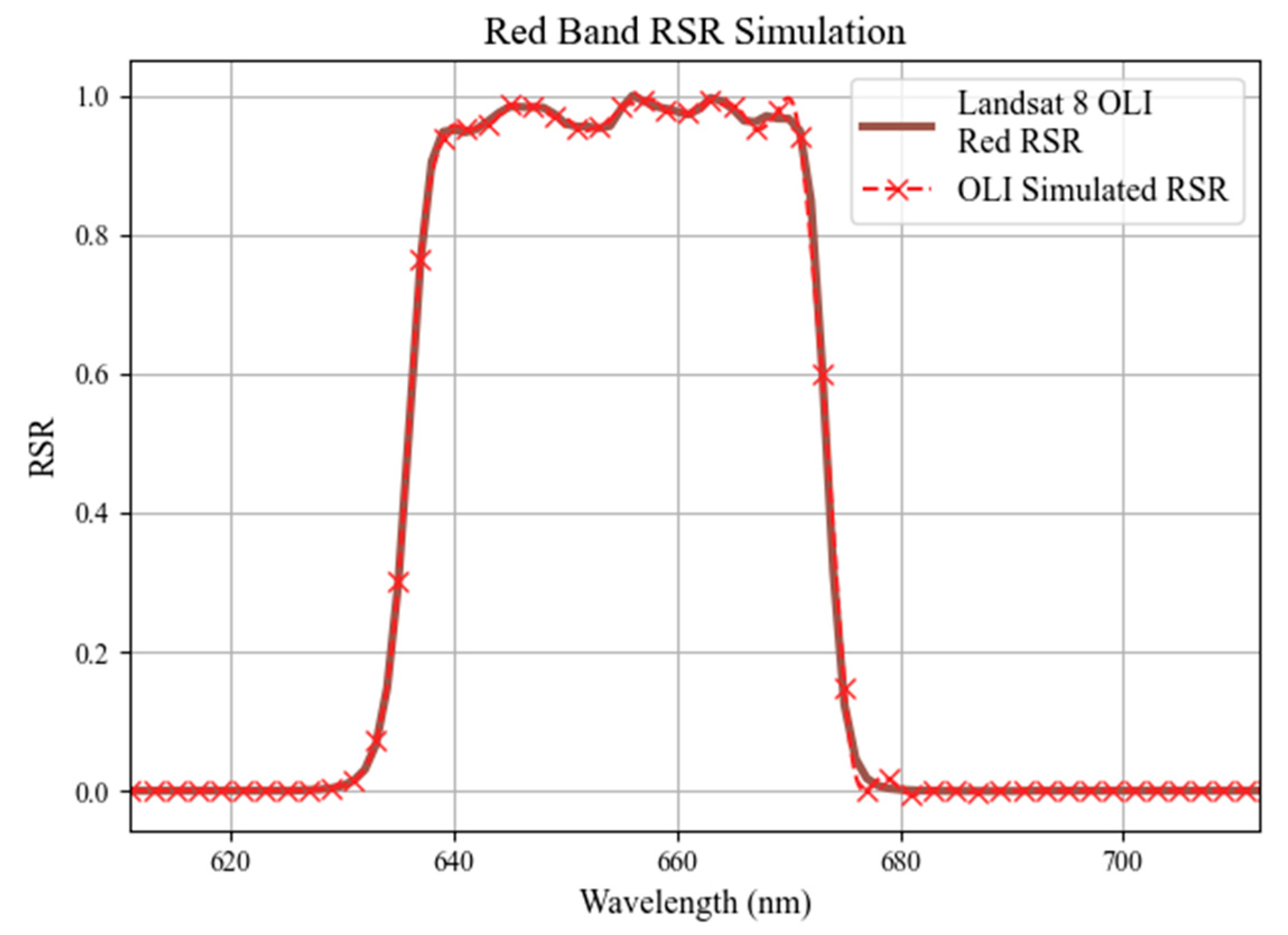
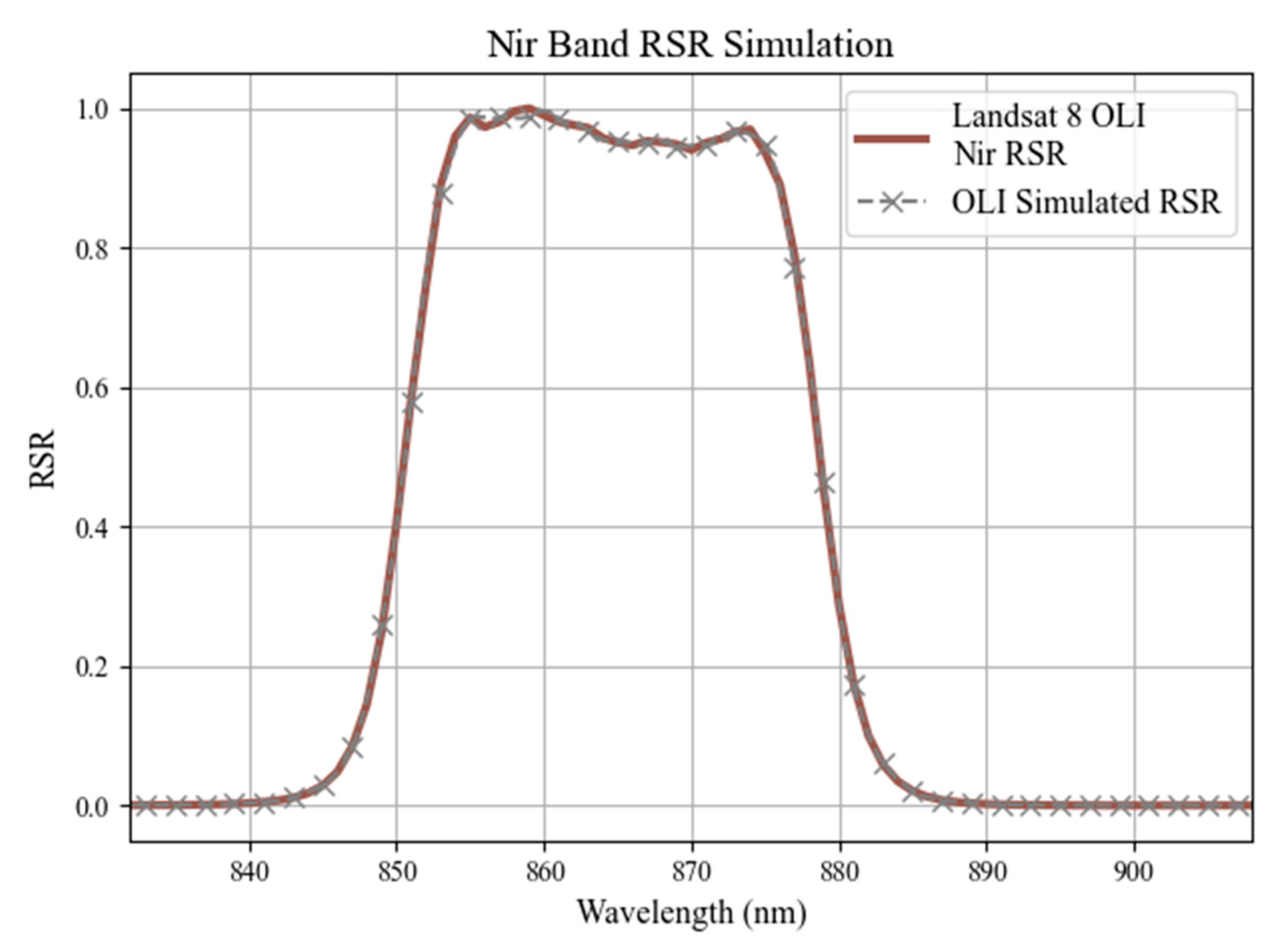
Lastly, this study also shows that an instrument like DESIS has fine enough spectral resolution and sampling to simulate RSRs that are almost identical to Landsat’s and could be usable for cross-calibration purposes.

References

- Brian, M.; Barsi, J.; Kvaran, G.; Ong, L.; Kaita, E.; Biggar, S.; Czapla-Myers, J.; Mishra, N.; Helder, D. Landsat-8 operational land imager radiometric calibration and stability. Remote Sens. 2014, 6, 12275–12308. [Google Scholar]
- Lamquin, N.; Woolliams, E.; Bruniquel, V.; Gascon, F.; Gorroño, J.; Govaerts, Y.; Leroy, V.; Lonjou, V.; Alhammoud, B.; Barsi, J.A.; et al. An inter-comparison exercise of Sentinel-2 radiometric validations assessed by independent expert groups. Remote Sens. Environ. 2019, 233, 111369. [Google Scholar] [CrossRef]
- Bouvet, M.; Thome, K.; Berthelot, B.; Bialek, A.; Czapla-Myers, J.; Fox, N.P.; Goryl, P.; Henry, P.; Ma, L.; Marcq, S.; et al. RadCalNet: A Radiometric Calibration Network for Earth Observing Imagers Operating in the Visible to Shortwave Infrared Spectral Range. Remote Sens. 2019, 11, 2401. [Google Scholar] [CrossRef]
- Fox, N.; Green, P.; Brindley, H.; Russel, J.; Smith, D.; Lobb, D.; Cutter, M.; Barnes, A. TRUTHS (Traceable Radiometry Underpinning Terrestrial- and Helio-Studies): A Mission to Achieve ‘Climate Quality’ Data. In Proceedings of the ESA Living Planet Symposium, Edinburgh, UK, 9–13 September 2013. [Google Scholar]
- Christopherson, J. An SLI Cross-Calibration Radiometer (SCR) Concept for Improved Calibration of Disaggregated Earth Observing Satellite Systems. In Proceedings of the JACIE Workshop, Reston, VA, USA, 26 September 2019. [Google Scholar]
- Krutz, D.; Müller, R.; Knodt, U.; Günther, B.; Walter, I.; Sebastian, I.; Säuberlich, T.; Reulke, R.; Carmona, E.; Eckardt, A.; et al. The Instrument Design of the DLR Earth Sensing Imaging Spectrometer (DESIS). Sensors 2019, 19, 1622. [Google Scholar] [CrossRef]
- Sebastian, I.; Krutz, D.; Eckardt, A.; Venus, H.; Walter, I.; Günther, B.; Neidhardt, M.; Reulke, R.; Müller, R.; Uhlig, M.; et al. On-ground calibration of DESIS: DLR’s Earth sensing imaging spectrometer for the International Space Stations (ISS). Proc. SPIE Opt. Sens. Detect. V 2018, 10680, 1068002. [Google Scholar] [CrossRef]
- Zhu, Z. Science of Landsat analysis ready data. Remote Sens. 2019, 11, 2166. [Google Scholar] [CrossRef]
- Wulder, M.A.; Loveland, T.R.; Roy, D.P.; Crawford, C.J.; Masek, J.G.; Woodcock, C.E.; Allen, R.G.; Anderson, M.C.; Belward, A.S.; Cohen, W.B.; et al. Current status of Landsat program, science, and applications. Remote Sens. Environ. 2019, 225, 127–147. [Google Scholar] [CrossRef]
- Knight, E.; Kvaran, G. Landsat-8 Operational Land Imager Design, Characterization and Performance. Remote Sens. 2014, 6, 10286–10305. [Google Scholar] [CrossRef]
- Morfitt, R.; Barsi, J.; Levy, R.; Markham, B.; Micijevic, E.; Ong, L.; Scaramuzza, P.; Vanderwerff, K. Landsat-8 Operational Land Imager (OLI) radiometric performance on-orbit. Remote Sens. 2015, 7, 2208–2237. [Google Scholar] [CrossRef]
- Thome, K.J. Absolute radiometric calibration of Landsat 7 ETM+ using the reflectance-based method. Remote Sens. Environ. 2001, 78, 27–38. [Google Scholar] [CrossRef]
- Czapla-Myers, J.; McCorkel, J.; Anderson, N.; Thome, K.; Biggar, S.; Helder, D.; Aaron, D.; Leigh, L.; Mishra, N. The Ground-Based Absolute Radiometric Calibration of Landsat 8 OLI. Remote Sens. 2015, 7, 600–626. [Google Scholar]
- Jorge, G.; Rodrigo, J.F.; Salvador, P.; Gómez, D.; Sanz, J.; Casanova, J.L. An empirical radiometric intercomparison methodology based on global simultaneous nadir overpasses applied to landsat 8 and Sentinel-2. Remote Sens. 2020, 12, 2736. [Google Scholar]
- Uprety, S.; Cao, C.; Xiong, X.; Blonski, S.; Wu, A.; Shao, X. Radiometric Intercomparison between Suomi-NPP VIIRS and Aqua MODIS Reflective Solar Bands Using Simultaneous Nadir Overpass in the Low Latitudes. J. Atmospheric Ocean. Technol. 2013, 30, 2720–2736. [Google Scholar]
- USGS. Prototype Satellite Cross-Calibration Radiometer (SCR) Workflow Algorithm Description Document (ADD) Using DESIS Hyperspectral and Landsat 8 Reference Imagery; United States Geological Survey: Reston, VA, USA, 2023; under review.
- Cosnefroy, H.; Leroy, M.; Briottet, X. Selection and Characterization of Saharan and Arabian Desert Sites for the Calibration of Optical Satellite Sensors. Remote Sens. Environ. 1996, 58, 101–114. [Google Scholar] [CrossRef]
- Helder, D.L.; Basnet, B.; Morstad, D.L. Optimized Identification of Worldwide Radiometric Pseudo-Invariant Calibration Sites. Can. J. Remote Sens. 2010, 36, 527–539. [Google Scholar] [CrossRef]
- Gorroño, J.; Banks, A.C.; Fox, N.P.; Underwood, C. Radiometric inter-sensor cross-calibration uncertainty using a traceable high accuracy reference hyperspectral imager. ISPRS J. Photogramm. Remote Sens. 2017, 130, 393–417. [Google Scholar]
- Li, S.; Ganguly, S.; Dungan, J.L.; Wang, W.; Nemani, R.R. Sentinel-2 MSI Radiometric Characterization and Cross-Calibration with Landsat-8 OLI. Adv. Remote Sens. 2017, 6, 147–159. [Google Scholar] [CrossRef]
- DESIS ATBD L1A, L1B, L1C, L2A Processors. Available online: https://www.tbe.com/en-us/what-we-do/markets/geospatial-solutions/DESIS/Documents/DESIS_Processing_Chain_and_Technical_Guide_atbd.pdf (accessed on 31 January 2023).
- Landsat 8 (L8) Data Users Handbook, Version 5.0, November 2019. Available online: https://d9-wret.s3.us-west-2.amazonaws.com/assets/palladium/production/s3fs-public/atoms/files/LSDS-1574_L8_Data_Users_Handbook-v5.0.pdf (accessed on 31 January 2023).
- Pagnutti, M. Simulating Virtual Satellite Constellations of Multispectral Imagers Using Hyperspectral Satellite and Airborne Imagery. In Proceedings of the JACIE Workshop, Reston, VA, USA, 24–26 September 2019. [Google Scholar]
- Burch, K. Simulation of Multispectral Imagers Using DESIS Hyperspectral Imagery for Harmonization of Satellite Constellations and Cross-Calibration. In Proceedings of the 1st DESIS User Workshop, Virtual, 28 September–1 October 2021. [Google Scholar]
- Ryan, R. Parametric Spectral Synthesis Errors of Hyperspectral Simulation of Multispectral Imagers. In Proceedings of the JACIE Workshop, Virtual, 10–13 January 2022. [Google Scholar]
- Alonso, K.; Bachmann, M.; Burch, K.; Carmona, E.; Cerra, D.; de los Reyes, R.; Dietrich, D.; Heiden, U.; Hölderlin, A.; Ickes, J.; et al. Data Products, Quality and Validation of the DLR Earth Sensing Imaging Spectrometer (DESIS). Sensors 2019, 19, 4471. [Google Scholar] [CrossRef]
- Hoja, D.; Schnieder, M.; Mueller, R.; Lehner, M.; Reinartz, P. Comparison of Orthorectification Methods Suitable for Rapid Mapping Using Direct Georeferencing and RPC for Optical Satellite Data. Int. Arch. Photogramm. Remote Sens. Spat. Inf. Sci. 2008, 37, 1617–1624. [Google Scholar]
- Hoge, W.S. A Subspace Identification Extension to the Phase Correlation Method. IEEE Trans. Med. Imaging 2003, 22, 277–280. [Google Scholar] [CrossRef]
- Keys, R.G. Cubic Convolution Interpolation for Digital Image Processing. IEEE Trans. Acoust. Speech Signal Process. 1981, 29, 1153–1160. [Google Scholar] [CrossRef]
- Pagnutti, M.; Blonski, S.; Cramer, M.; Helder, D.; Holekamp, K.; Honkavaara, E.; Ryan, R. Targets, methods, and sites for assessing the in-flight spatial resolution of electro-optical data products. Can. J. Remote Sens. 2010, 36, 583–601. [Google Scholar]
- Malone, K.J.; Schrein, R.J.; Bradley, M.S.; Irwin, R.; Berdanier, B.N.; Donley, E. Landsat 9 OLI 2 Focal Plane Subsystem: Design, Performance, and Status. In Proceedings of the Earth Observing Systems XXII; Butler, J.J., Xiong, X., Gu, X., Eds.; SPIE: San Diego, CA, USA, 2017; p. 5. [Google Scholar]
- Dabney, P.W.; Levy, R.; Ong, L.; Waluschka, E.; Grochocki, F. Ghosting and Stray-Light Performance Assessment of the Landsat Data Continuity Mission’s (LDCM) Operational Land Imager (OLI); Butler, J.J., Xiong, X., Gu, X., Eds.; SPIE: San Diego, CA, USA, 2013; p. 88661E. [Google Scholar]
- Saul, A.T.; Flannery, B.P.; Press, W.H.; Vetterling, W.T. Numerical recipes in C. SMR 1992, 693, 59–70. [Google Scholar]
Figure 1.
SCR and client/reference instrument calibrations needed to meet radiometric uncertainty goals.
Figure 2.
Cross-calibration steps that transfer calibration from a reference satellite (L8) to an SCR (using DESIS as surrogate).
Figure 3.
Solar and sensor view angles for the DESIS/L8 OLI image pair over Oklahoma (L8 P27/R36 and DESIS Tile 8). DESIS scene boundaries are outlined in red and shown against the L8 OLI scene.
Figure 4.
L8 OLI coastal aerosol B01 simulated using DESIS hyperspectral bandpasses. The figure shows scaled DESIS hyperspectral bands, the simulated multispectral band, and the actual L8 spectral response.
Figure 5.
L8 coastal aerosol B01 actual and simulated using DESIS.
Figure 6.
L8 blue B02 actual and simulated using DESIS.
Figure 7.
L8 green B03 actual and simulated using DESIS.
Figure 8.
L8 red B04 actual and simulated using DESIS.
Figure 9.
L8 NIR B05 actual and simulated using DESIS.
Figure 10.
Coastal aerosol band regression example over Oklahoma (L8 P27/R36 and DESIS tile 8).
Figure 11.
Blue band regression example over Oklahoma (L8 P27/R36 and DESIS tile 8).
Figure 12.
Green band regression example over Oklahoma (L8 P27/R36 and DESIS tile 8).
Figure 13.
Red band regression example over Oklahoma (L8 P27/R36 and DESIS tile 8).
Figure 14.
NIR band regression example over Oklahoma (L8 P27/R36 and DESIS tile 8).
Figure 15.
GSD influence on cross-calibration results.
Figure 16.
dependence on SCR-client (or SCR-reference) overlap area for SCR GSDs varying from 30 m to 480 m.
Figure 17.
Independent spatial samples’ influence on cross-calibration gain uncertainty.
Figure 18.
Misregistration influence on cross-calibration results.
Figure 19.
PSF influence on cross-calibration results.
Figure 20.
Effect of misregistration and image blur on regression quality of fit.