1. Introduction
Nowadays, there are a large number of 3D sensors based on different measurement principles. The accuracy and the number of measurements that such a sensor can perform in a given time have increased enormously in recent years. However, the processing of the collected data could not keep up with the given pace. For this reason, the demand for 3D data processing is extremely high. The range of interest extends from autonomous driving [
1,
2,
3] to infrastructure mapping [
4,
5,
6,
7] up to biomedical analysis [
8].
In most cases, point clouds are used to define the collected 3D data. The processing of point clouds has several disadvantages compared to images, for instance. First of all, point clouds are very sparse, and most of the environment that may have been covered is empty. Furthermore, the density of the points within the same point cloud varies. Commonly, the point density close to the sensor is denser than the point density further away from it. Thirdly, point clouds are irregular. This means the number of points within a respective point cloud differs. Moreover, point clouds are unstructured, which implies that each point is independent and the distance between adjacent points varies. In addition to that, point clouds are unordered and invariant to permutation.
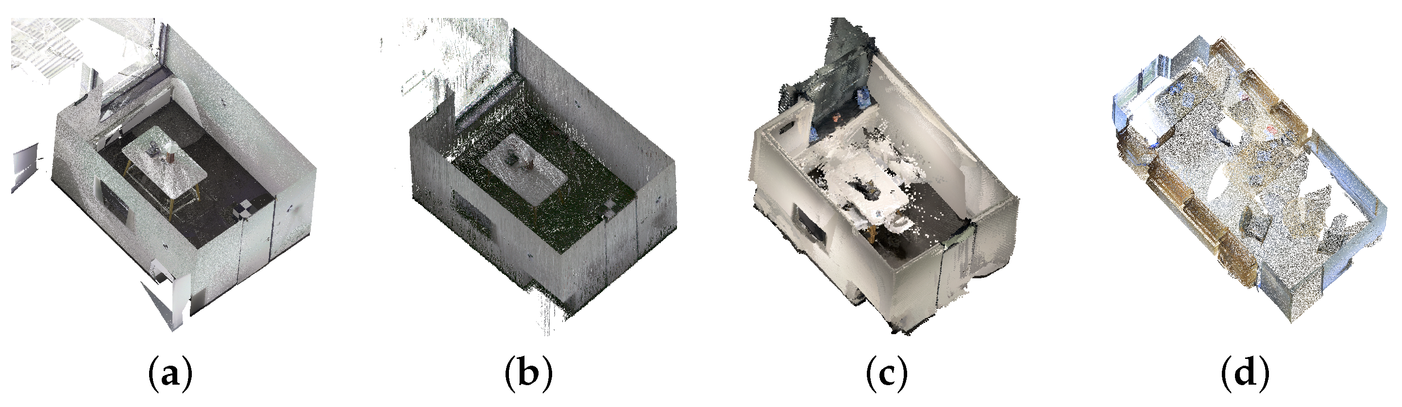
Each 3D sensor produces data with different characteristics, resolutions, and noise levels. This makes it challenging to process and analyze the data without changing the applied methods or algorithms. In order to cover as many of the sensors used today as possible, it must be ensured that the methods or algorithms generalize. An example of four different point clouds received by four different sensors is shown in
Figure 1. It can be seen that not only are the colors displayed differently, but also the point density and the geometries are different. Especially with the windows, the difference is most obvious. In the first two sensors, the glass pane is barely visible in the point cloud while, in the rear two sensors, it is completely visible.
Despite the disadvantages mentioned, point clouds have enormous potential due to their high information content. The idea of Scan-to-BIM [
9], a process of creating a 3D model from point cloud data obtained by laser scanning or other types of 3D scanning technologies, was born because of the high information content. The goal of Scan-to-BIM is to extract accurate and detailed 3D building models from point cloud data, which can be used for a variety of applications, such as building renovation, construction management, and facility management. Ideally, the digital model is as similar to the real object as possible. In case the real object changes within time or the object does not even have such a digital repository, the idea of Scan-to-BIM is to make use of 3D sensors to generate the digital BIM. Today, a common way is to manually extract the information out of the 3D data and create the model by hand. This procedure can be, depending on the size and complexity of the object, very time-consuming.
The main purpose of this work is to automate the idea of Scan-to-BIM as much as possible without depending on a specific sensor. With the generalization to different 3D sensors, limited work is currently being performed. The current state of the art often necessitates a particular sensor or is specialized for a segment of the pathway from the point cloud to the geometric model. For this purpose, this paper can be divided into five parts. First, to handle large scenes as well, we have to downsample and unify the given point cloud. This makes it possible to partially compensate for the initial differences between the sensors in terms of point density. To keep as much geometrical information as possible, we introduce a feature-preserving downsampling strategy. In the second part, we make use of a Neural Network (NN) to segment the preprocessed points into relevant classes. In our case, we are only interested in the following classes: floor, ceiling, wall, door, door leaf, window, and clutter, as these are sufficient to describe the main structure of the building. The segmented point cloud is divided into potential room candidates within the next step. This way, the more complex room reconstruction can be applied to the smaller subsets containing only the points belonging to the room itself. In the fourth step, the polygons are fitted into the room candidates in order to, on the one hand, further reduce the point cloud and, on the other hand, to bring the point cloud into a more readable output format. The last step expands the reconstructed room by adding architectural features. For the first experiment, we focused on windows and doors. Of course, this approach can be extended to other objects as well.
2. Related Work
The current state-of-the-art techniques for Scan-to-BIM typically involve using a combination of machine learning and computer vision techniques to extract building components. Methods such as edge detection, feature matching, and region growing are used to extract features from the point cloud data, which can then be used to segment the point cloud data into different building components. In [
10], 2.5D plans are extracted from laser scans by triangulating a 2D sampling of the wall positions and separating these triangles into interior and exterior sets. The boundary lines between the sets are used to define the walls. Within [
11], the wall candidates are extracted by heat propagation to allow the fitting of polygons. However, both approaches only allow the fitting of environments with single ceilings and floors and do not detect further attributes. In [
12], parametric building models with additional features are reconstructed from indoor scans by deriving wall candidates from vertical surfaces observed in the scans and detecting for wall openings. Combining supervised and unsupervised methods was performed by [
13,
14,
15]. In the former, a semi-automatic approach for reconstructing heritage buildings from point clouds using a random forest classifier combined with a subpart annotated by a human was introduced. The second work first cleans the point cloud and samples new relevant points, in the preprocessing step, followed by creating a depth image and detecting the walls and doors using a Convolutional Neural Network (CNN). The last uses a 3D NN to classify the points and to extract the surfaces afterward.
In [
16], the blueprint was analyzed to detect walls to further use them to extract rooms. The study in [
17] extracts geometric information for buildings from Manhattan-world urban scenes, which states that these scenes were built on a Cartesian grid [
18]. The problem of reconstructing polygons from point clouds is formulated as a binary optimization problem by using a set of face candidates in [
19].
To tackle the task of 3D segmentation, there are different approaches today. A general overview is given in [
20]. Mainly, these approaches can be divided into projection-based, discretization-based, and point-based methods. For the segmentation part, we made use of three different architectures and compared them in terms of generalization. Two of the selected approaches are point-based and one is a discretization-based method. We made use of RandLA-Net [
21], where the authors made use of pointwise Multilayer Perceptron (MLP) to learn 3D features directly from the point cloud, as well as to downsample the point cloud. Point Transformer [
22] belongs to the same category as RandLA-Net, but the authors made use of self-attention, which is intrinsically a set operator and, therefore, matches 3D point clouds that are essentially sets of points with positional attributes. Due to the fact that all the relevant classes are large, we decided to make use of a 3D convolution as well. For the base structure, the U-Net [
23] architecture will be used.
To make our algorithm as applicable as possible, we tried to avoid any dependency on the used 3D sensor. This means we cannot rely on further point features, like colors or reflections, and have to focus on the pure geometrical output. In [
24], geometrical features based on the eigenvalues
,
, and
of the covariance matrix in a given neighborhood with
are used to describe the local 3D structure. In [
25], these features are used to detect contours within large-scale data.
3. Method
3.1. Feature-Enriched Downsampling
We used a voxel grid downsampling to reduce the number of points and to allow for a more uniform distribution. To preserve the geometrical information, we used the downsampling procedure to calculate the geometrical features. Each voxel defines the neighborhood of the given points to avoid the use of searching for nearest neighbors. The covariance matrix
is calculated for each voxel with the position
,
, and
in the given 3D environment:
with
and the
n points within the voxel. The features are defined by [
24] and are summarized in
Table 1.
The results from our described downsampling strategy are
with
m new points. The procedure is shown in
Figure 2.
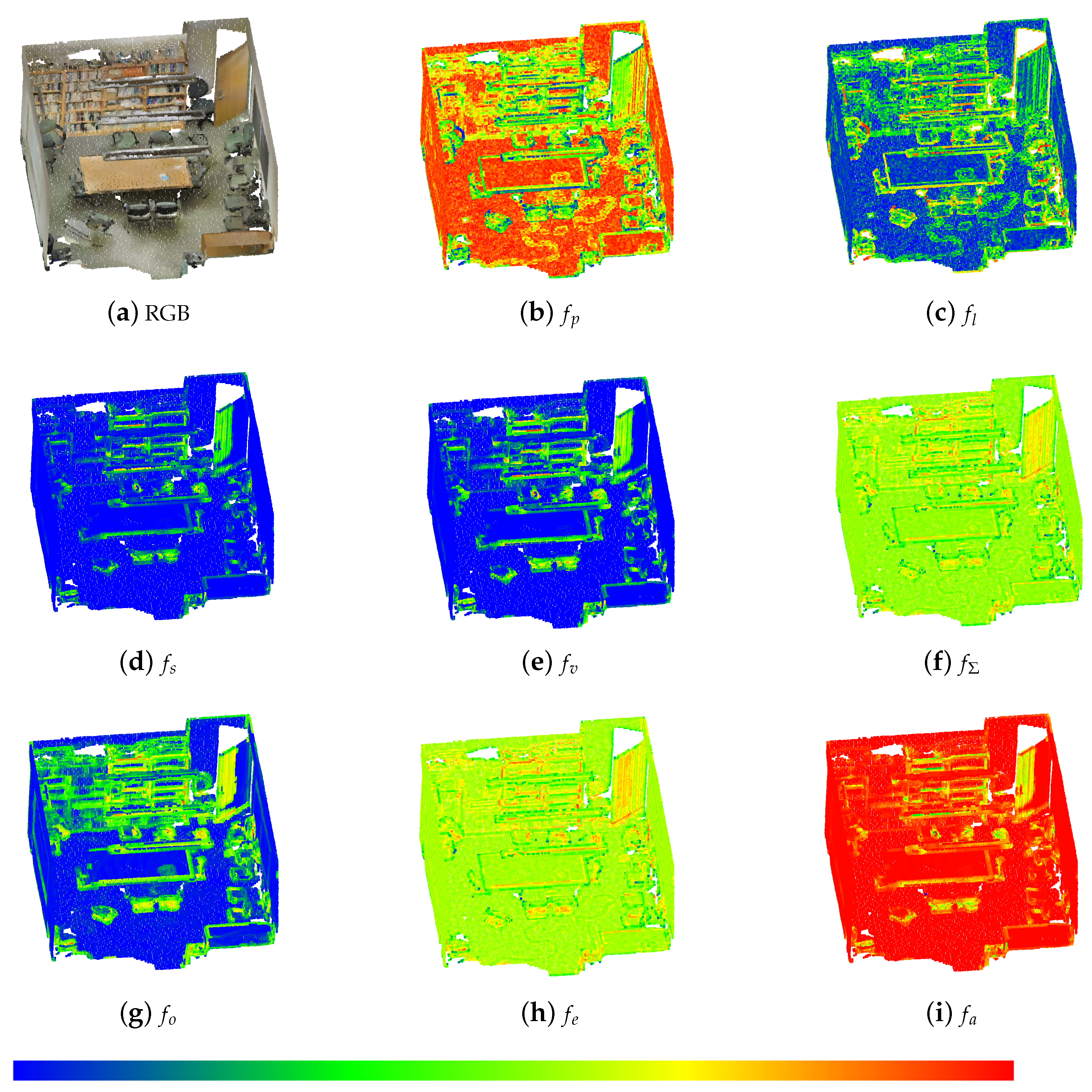
The calculated covariance matrices depend on the size of the voxels. For this reason, we scale the calculated eigenvalues with the voxel size . Further, we perform a linear transformation to the final features to receive scaled features within the range .
3.2. Semantic Segmentation
To describe a room, only a few classes are needed. Therefore, we are only interested in knowing the following classes: floor, ceiling, wall, door, door leaf, window, and clutter. For the classes door and window, only the frame around the opening is relevant and not the actual panel or glass.
The input for the NN is the point cloud, where each point is represented by its 3D coordinates and the features described in the previous chapter. The voxel size for downsampling and feature computation was set to 10 cm. We chose this size to be able to compute the features even in less dense point clouds and because the classes relevant to us can still be described with this resolution.
For the choice of the parameter of the architectures, we have followed as closely as possible the specifications in the respective publications. For the point-based methods, we choose the following downsampling rates: . In contrast, the per-point feature dimension was increased for each layer: . For the discretization-based method, we halved the grid size after every layer and doubled the feature dimension starting with 32.
3.3. Regions of Interest
To find potential room candidates, all points except points belonging to walls are removed from the predicted point cloud. We do not need high resolution for this part and temporarily reduce the remaining wall points further. By using the assumption of walls being perpendicular to the ground plane, we can reduce the dimension by projecting all points into the x-y plane. The basic idea behind our algorithm is following the line until we reach the same point again.
To perform this, we transform the points into an undirected graph . Each remaining point is described by a node with n points. We build the graph iteratively starting at a random point and allow to only connect to the closest point. The selected closest point is removed from the selectable points and defines the new start. The resulting edges have the corresponding weight , where d is the Euclidean distance .
Due to the way the graph has been constructed, the distance between two associated nodes may be much higher than the actual underlying neighboring point. To resolve the incorrect assignment, all connections with with are removed and, this way, the whole graph is divided into subgraphs .
All nodes are used to rebuild with more suitable edges. A distance matrix with is calculated with . Next, all nodes i and j with that are not within the same subgraph , or have at least a path length with more than 10 nodes, are connected with each other. Note that the newly created graph can have nodes with more than two edges. All subgraphs that have only a single node are considered an outlier and are removed. The remaining nodes with a single edge are connected in case there is a node with a distance with and a path length with more than 10 nodes.
Cycles within
are an indicator of potential room candidates. To find the shortest cycles within
, we select a random node
and temporarily remove the edge
. To check whether a circle exists, the Dijkstra algorithm [
26] is used to find the path
. If a path
exists, it most probably describes a room candidate
. The algorithm is shown in Algorithm 1.
| Algorithm 1 Find shortest cycle in graph |
- Require:
- Ensure:
return
|
Each detected cycle is analyzed and the area of the polygon described by the nodes is calculated. We make use of formulation described in [
27]:
with
n points and
. Rooms with an
are considered as outliers and removed.
3.4. 3D Room Reconstruction
The following procedure will be performed on each potential room candidate separately. This means that the reconstruction only has to process easier subparts instead of the entire point cloud. We retain the assumption made in
Section 3.3 for the first step.
We use RANSAC [
28] to fit
of the points within the defined contour with lines. All points that belong to the defined line are used in the later processing. This way, we can use the points to calculate the root mean squared error
between the fitted plane and the assigned points; to define how good the fit is, we can bound the height for a face by the given z-values and can calculate how well the line is covered by points.
The fitted lines are bounded into segments by using the containing points. In case of a jump larger than some threshold, the line segment is split. A jump is detected by sorting the distance between one bounding point and all points lying on the segment in ascending order. In case of a large gradient , a jump is detected.
The cosine similarity between the direction vectors of the segments is used to check for parallel segments. In case of two line segments being parallel with a distance m, where the bounds of the smaller segment are covered fully by the bounds of the larger one, the smaller segments are removed.
The remaining line segments are used to search for intersections. To make sure intersections for line segments are possible, we increase the length of each segment in both directions (
,
) by
:
Since line segment k might be intersected by multiple other segments, each intersection point is stored in . In the case of the bounding points of k being close to one of the intersecting points, , the bounding is replaced by the intersecting point. Otherwise, the bounding points are added to the set as well. The line segment k, as well as the points lying on the segment, are divided into new segments.
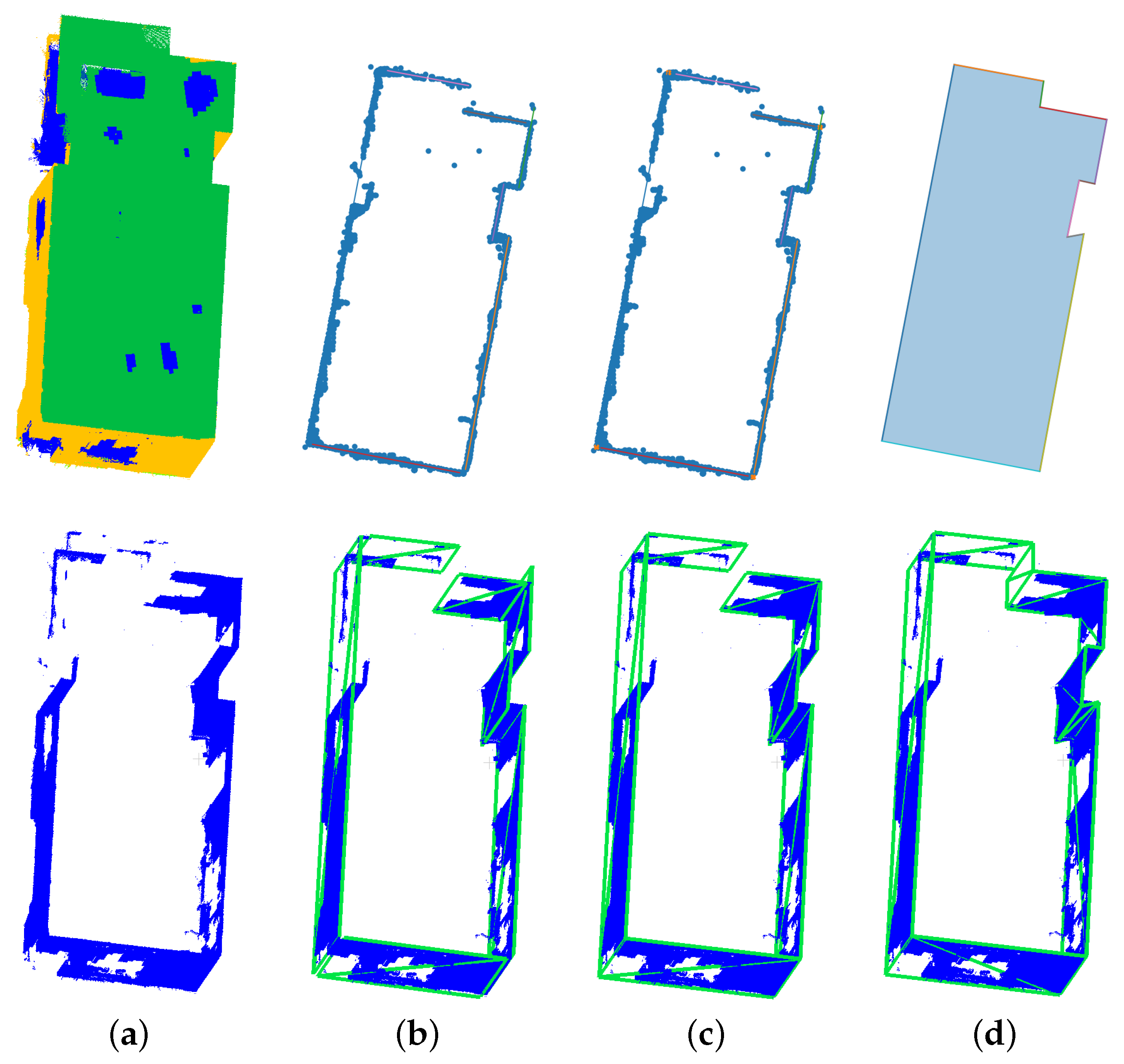
The idea of following the line is used to generate the final path contour. In case the angle between two connected segments
is smaller than
, the two segments are fused and refined. The value was selected because acute angles in the construction industry are rather atypical. The described procedure is visualized in
Figure 3.
The next step is to close the wall faces with the corresponding ceiling and ground. The procedure for bounding the wall to the ceiling and the ground is equivalent. For this reason, we will describe this for the ceiling points in the following manner.
We use RANSAC to fit the largest plane into the points belonging to the class ceiling. The height for each face is calculated by the intersection of the lines defining the wall faces with the detected plane. For the outlining contour, describing the room is already known, we create an n-Gon by the intersection points. In case the detected room does not have a sufficient number of points belonging to the floor or the ceiling, the detected room is rejected. This can occur if, for example, an inner courtyard or reflections within a room have been incorrectly detected.
3.5. Projecting Additional Architectural Features
As we defined further classes, like openings, which can indicate a
door or a
window, we can fit them into the polygon as well. Within each room candidate, we create instances for the classes
window and
doors by using a clustering algorithm DBSCAN [
29]. Afterward, we create a Bounding Box (BB) around each instance and create cuboids out of it. Since we do not assume that the points are axis-aligned, we make use of the Principal Component Analysis [
30] to create an Oriented Bounding Box (OBB) from the orthographic perspective. By using this perspective, we reduce the 3D problem to a 2D one since we only use the
x and
y values to calculate the covariance matrix. The min and max values of
z are used to define the height of the OBB. One has to keep in mind that, due to this assumption, windows in roof slopes, for instance, cannot be described precisely.
4. Experiments
We studied the behavior of our proposed workflow on different data sources from real-world scenarios to verify generalization. For this reason, we used data from different sensors and different environments. The S3DIS dataset [
31], where the data are collected by a Matterport Camera, shows three different buildings of mainly educational and office use. The Redwood dataset [
32] offers an apartment that is reconstructed from RGB-D video. The sensor manufacturer NavVis provides an example point cloud created from their sensor VLX [
33]. Further, we used the RTC360 and the BLK2GO developed by Leica Geosystems AG to record two different indoor scenes within Freiburg. One is a public building and the other one is a typical German apartment. We added more reconstructed buildings from the ISPRS benchmark [
34] into
Appendix A.
4.1. Feature-Enriched Downsampling
We compared our implementation for downsampling with the simultaneous calculation of the geometric features with the downsampling version of Open3D [
35]. Likewise, we computed the k Nearest Neighbor (kNN) with the library Scikit-Learn [
36] and Open3D to compare the runtimes. We show the results in
Table 2. At this point, it should be mentioned that in the computation time of the kNN, in contrast to our implementation, the eigenvalues of the covariance matrices have not yet been computed. In summary, the downsampling time triples, but we have an approximation of the geometric properties in this area that would otherwise be lost. The resulting features are visualized in
Figure 4.
4.2. Network Generalization
All networks are trained on the S3DIS dataset using Area 5 for validation. For generalization purposes, we further collected and annotated some of our own data by using the RTC360 scanner. We selected these two different types of sensors because the point clouds highly differ. As mentioned earlier, we are not interested in furniture and other objects but in the actual structural elements of the building. For this reason, we moved all irrelevant classes. The class beam is moved into ceiling, column is moved into wall, and the remaining classes are moved into clutter. To receive the actual opening for the door, we split the class door into two classes: door and door leaf. For the evaluation of each model, we used the mean Intersection over Union (mIoU).
As the classes within the datasets are highly imbalanced, we will use a weight for each class
leading to the weighted cross-entropy loss
:
To avoid overfitting, the data is augmented. First, we dropped a random amount of points. Afterward, the x, y, and z position of each point is shifted by the value of , the point cloud is rotated around the z-axis by an angle between 30° and 330°, each point cloud is scaled by a value of , and we add noise with . Each augmentation but the first is applied independently with a probability of . Since the data from S3DIS in the original format are divided into rooms, but we also want to apply the learned network to the individual viewpoints of the scanner, we have divided the entire point cloud from one area into random parts. This way, we have point clouds that have several rooms, or at least parts of them, in a single scan.
The training and different evaluation results are shown in
Table 3. The first thing to mention is that using the calculated geometric feature instead of the color improves the result for the classes relevant to us. This means that all the architectures used can recognize patterns based on geometry alone and there is no need for color information. Another important point is that the windows are not properly recognizable using either the color or the geometric feature when the data is captured by a different sensor. This point counts for all NNs used and indicates that the geometry must be too different in the data itself.
Since the approach using 3D convolutions combined with the geometrical features generalized the best, we will use it for the ongoing pipeline. Keep in mind that all of the networks might be further optimized and different architectures can be used as well, but this is not the main focus of our work.
4.3. Regions of Interest
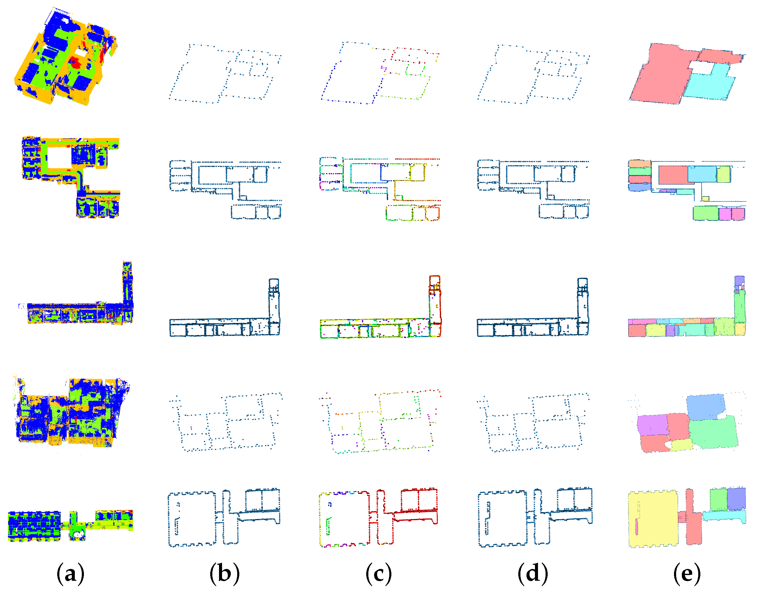
For generalization, we applied the algorithm to all the named datasets. As our models were trained on the S3DIS data, we only applied our method to the unseen validation set (Area 5) and merged the separated rooms to remove any prior knowledge. Further, we did not axis-align the point cloud nor remove the reflections for the RTC360 and BLK2Go data. The results can be seen in
Figure 5 and
Table 4. Each row shows a different dataset and sensor. The Redwood, the S3DIS, the RTC360, the BLK2Go, and the VLX data are displayed in order. The first column shows the prediction, and the second is the first step of the created graph followed by the separated, and in different colors, visualized subgraphs. The third column shows the reconnected graph that allows nodes to have more than two edges. The final contour, described by the detected cycles, is shown in the last column.
We would like to emphasize that the algorithm was able to recognize the rooms even under a bad prediction (BLK2Go). The hallway in the S3DIS data was not detected, but it was not closed either since we separated only a part of it from the data. One can see the output for the whole of Area 5 in
Appendix A.
The post-processing simply checks the number of points belonging to the classes ceiling and floor. In case the detected room does not have a ceiling or a floor, it is rejected, as it might belong to an inner courtyard, or it was created due to reflections.
Table 4 clears that up; after the post-processing, the algorithm was capable of detecting all the given rooms without any prior knowledge except for the RTC360 data. There is a lot of clutter in the long hallway of the building. This has resulted in large gaps in the walls and shallow predictions, making it difficult for the graph to compensate. In cases where the resulting gap in the walls is larger than the width of the hallway, the graph may close the hallway at that point. For this reason, the hallway in the building has been divided into six sections instead of three.
4.4. 3D Room Reconstruction
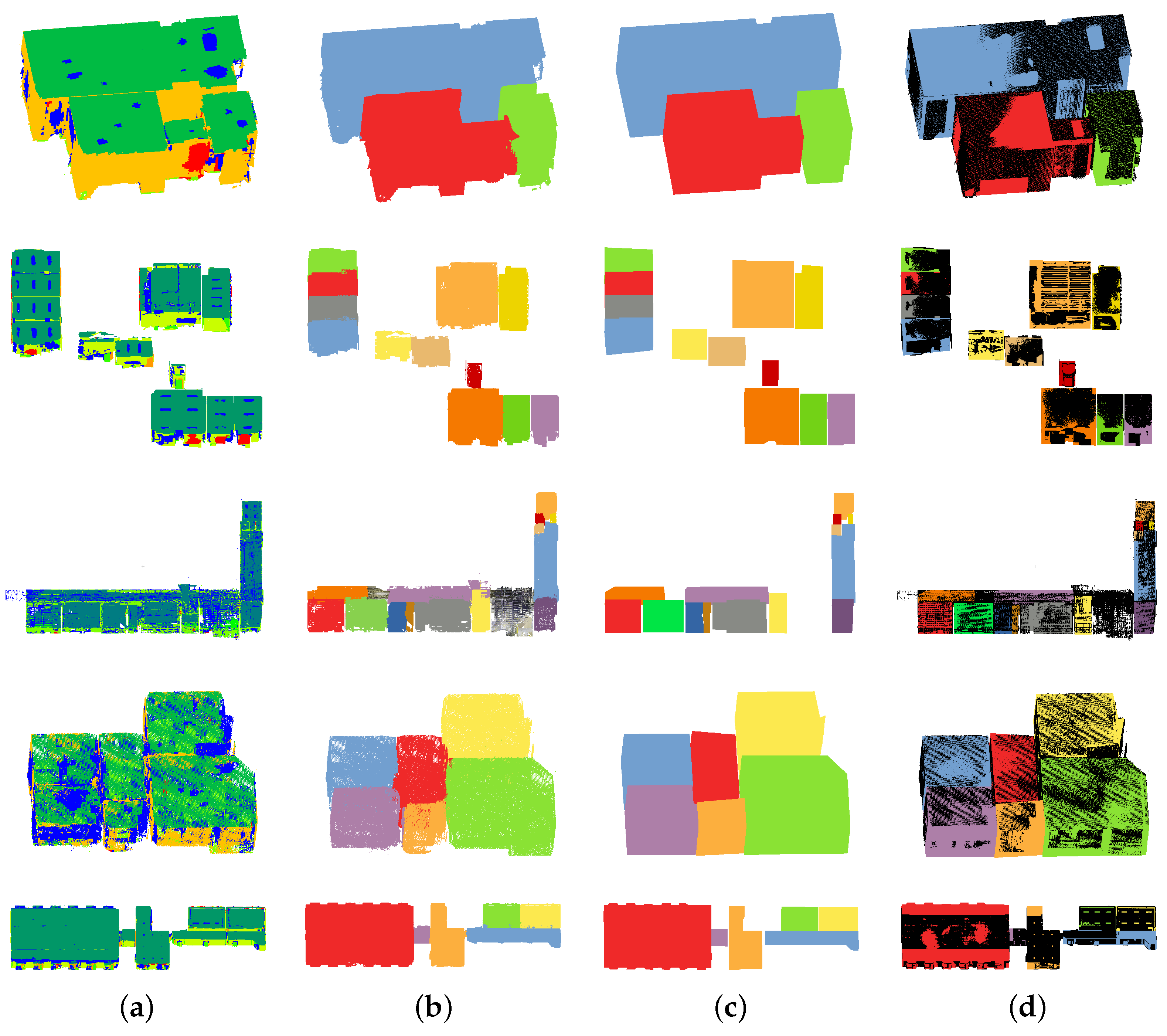
All the detected room candidates for the different datasets are reconstructed and shown in
Figure 6. We ordered the rows in the same way as described in
Section 4.3. The first column shows the full prediction. All the points belonging to the same contour detected by our proposed graph algorithm are colored in the same color in column two. This is the input to the described room reconstruction algorithm. The output generated by the room reconstruction is shown in the third column. The last column shows the raw input point cloud and the reconstructed rooms together.
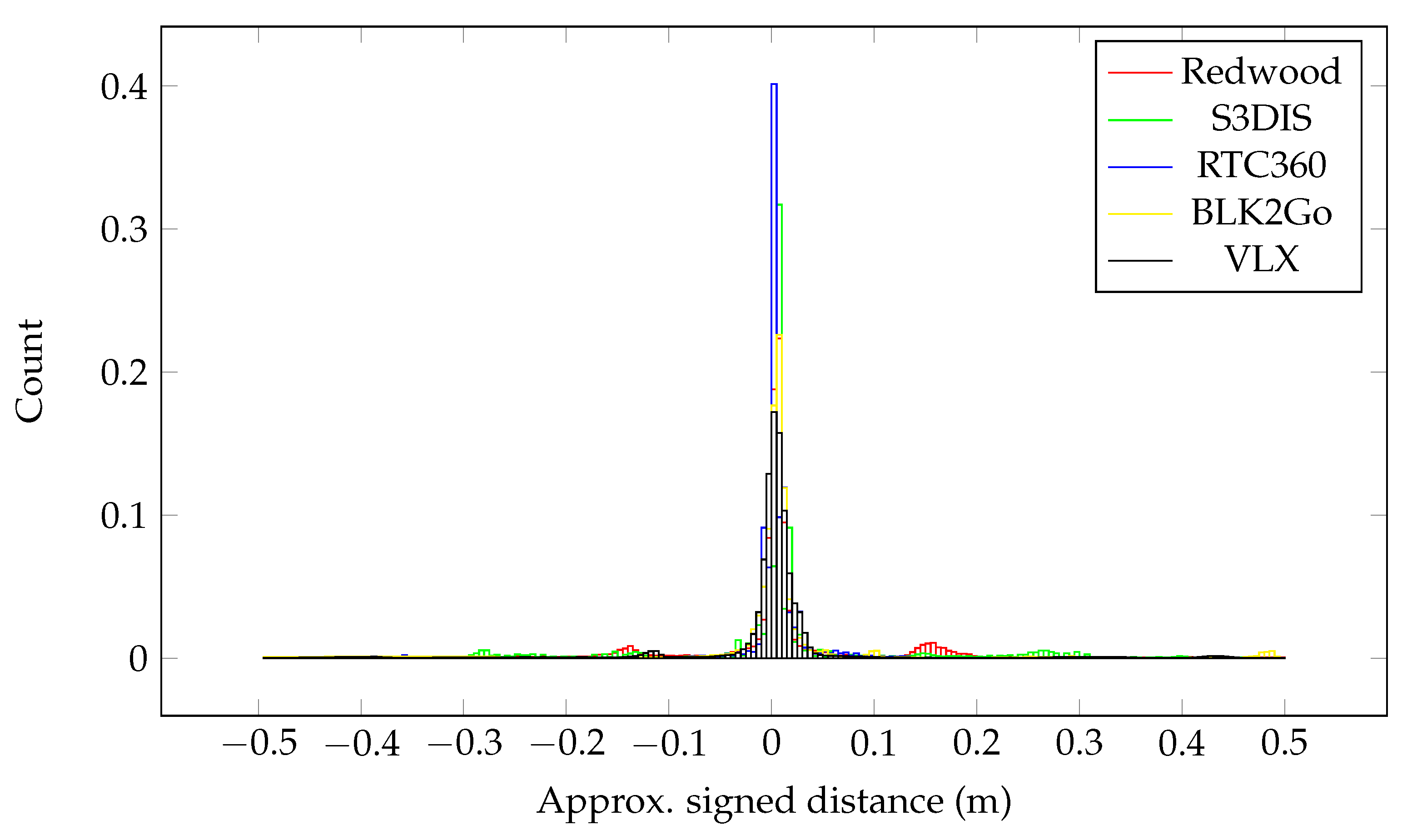
To easily analyze the accuracy of the reconstruction process, the point cloud to mesh distance is calculated for the extracted rooms and the points that were used for the extraction (ceiling, ground, and wall). Note that this is not equivalent to the ground truth geometry of the rooms, but serves as an indicator of how well the process describes the given points. The histograms for the distribution of the calculated distances are shown in
Figure 7. In all cases, the distance between the reconstructed spaces and the points is very small. There is a second peak in the Redwood data. This can be explained by the fact that one room has two different ceiling heights, of which the smaller one is neglected, resulting in several points being incorrectly described.
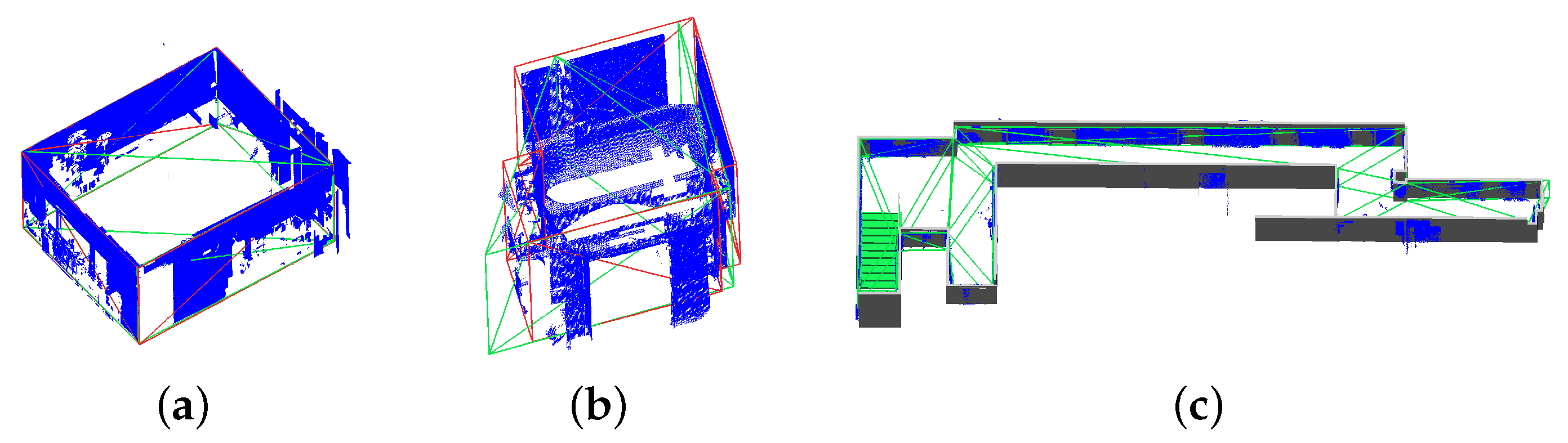
To investigate how accurate the reconstruction actually is, we took a closer look at three different rooms. We manually reconstructed two rooms and exported one that was given by the ISPRS benchmark. The result is shown in
Figure 8. The automatic reconstruction is shown in green, the ground truth in red and gray, and the points that have been detected as a wall are displayed in blue. It is noticeable that small edges are not taken into account by the algorithm. This is because not all the wall points are used for the reconstruction and the way RANSAC does fits the points. The threshold of not using all the points for the characterization of the geometry is a trade-off between the use of possible wrong predictions and the neglect of small details.
4.5. Additional Features
As shown in
Table 3, the networks are generalizing well for the classes
ceiling,
floor, and
wall, which allows the following algorithms to reconstruct the 3D room. Even if the openings of the doors are not detected with the same IoU as the previous classes, it is possible for the algorithm to describe the openings for different sensors. Nevertheless, it shows a lack of generalization for the class
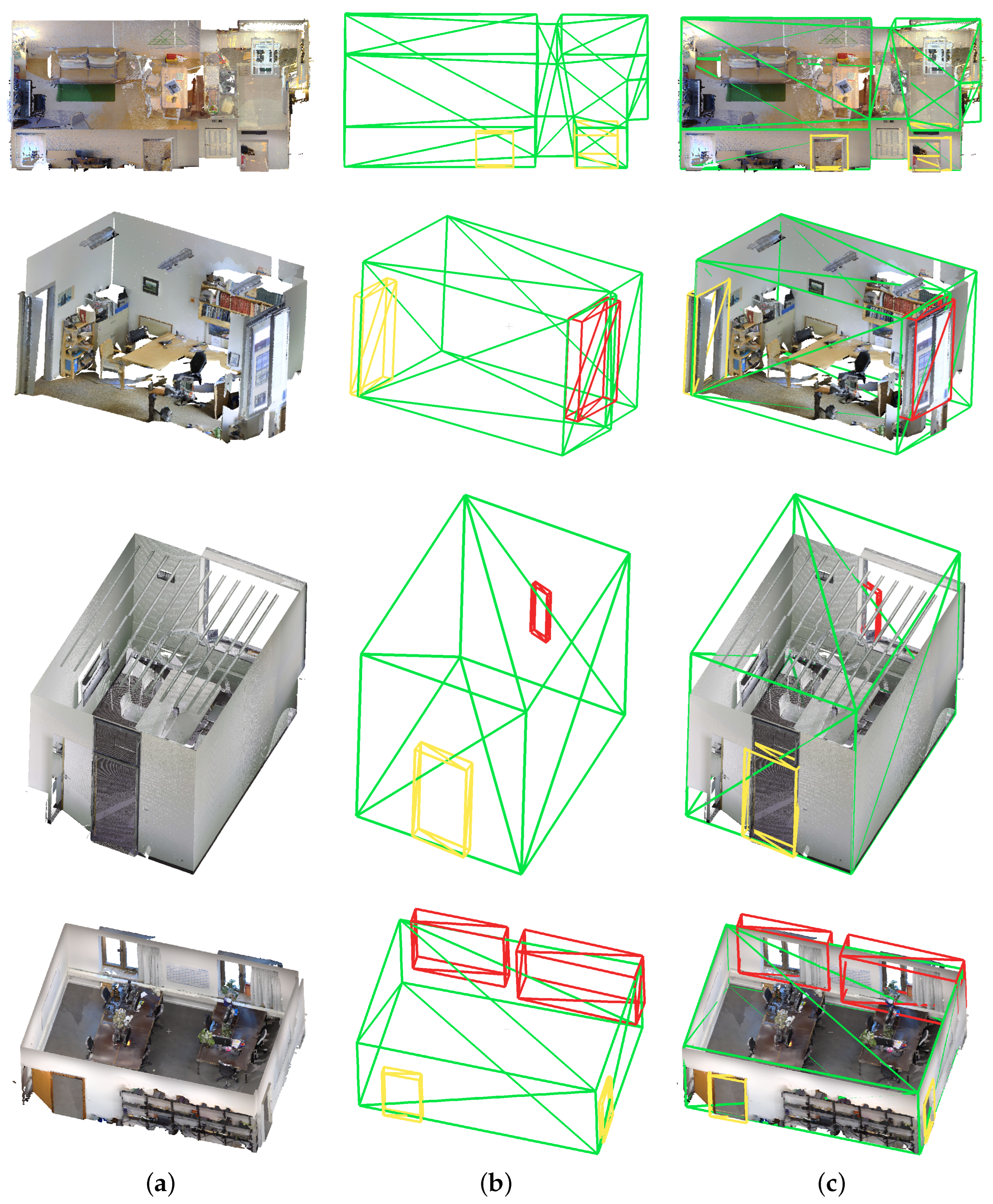
window. Class recognition is only applicable to the data recorded with the same sensor. Example results for each sensor are shown in
Figure 9.
The main reason for the class
window not being detected in other datasets is the geometry captured. As mentioned in
Section 1, the point cloud depends on the sensor. In
Figure 1, we have illustrated the difference. If we look at the window, it is clear that it has different geometries depending on the sensor. The laser sensors used by Leica Geosystems measure through the glass in the windows and a window is, thus, primarily described as a hole in the wall. In contrast, the matterport used in the acquisition of the S3DIS dataset captures points on the window itself. The defined window is, thus, not described by an opening, but by an offset plane to the wall.
4.6. Limitations
In this section, we would like to discuss the limiting factors. Since the pipeline is based on the detection of walls, and we assume that a room is closed by walls, the procedure only works if a sufficient number of points for the walls has been detected. This leads to problems as soon as a wall consists only of windows. Even if windows and doors are included in the description of the room, it can happen that there are too few points and the graph does not recognize the room as closed. Corridors, like the one from the S3DIS dataset in
Appendix A, which have neither a defined beginning nor a defined end, cannot be closed with the graph either. This is because the graph, when running along the outer walls, never arrives at the inner walls of the corridor, but at its original beginning. Thus, only one large room, which theoretically includes all the rooms inside the corridor, would be included. It follows that the graph as implemented is not able to recognize rooms that are enclosed on all sides by another room.
The graph itself is also able to recognize rooms with round walls. However, since the reconstruction based on it currently only allows planes and combines them if the angles are too small, round walls cannot be reconstructed. During reconstruction, each room is considered separately, so that rooms with different ceiling and floor heights can be described. However, only one ceiling and floor is allowed per room. For this reason, no roof slopes and no rooms that go over several floors can be described.
5. Discussion
The large number of available 3D sensors makes it possible to address different applications. However, the most common format, the point cloud, is mostly not usable by the consumer. We have developed a method that is intended for the use case of interiors and brings the point cloud into a minimal geometric format while preserving architectural properties.
We have tested our method on five different real-world datasets collected by five different sensors. The scenes used have been selected to be as realistic as possible. This means that all the recorded rooms are inhabited and, therefore, furnished and cluttered. We chose data from different continents showing apartments, educational rooms, and offices. Not only the data but also the sensors vary greatly in their characteristics. This way, we are able to show how far our approach generalizes and, thus, offer a wide range of applications.
In this work, it has been shown that the difference between the sensors is not insignificant and, even if the focus is put on the 3D geometry alone, the differences have a direct influence on the trained NN. This means that the recognition of the trained classes is not transferable to all the classes. In our case, the windows would have to be mentioned at this point. Nevertheless, the generalization for the recognition of the remaining classes could be proven and, thus, the NN represents a suitable basis for the separation and filtering of the 3D data.
In most cases, the graph detected the correct number of rooms and was able to reduce the number of points used for the polygon. Other advantages of the method are that it provides direct information about the area size of the rooms, there is no limitation to the planar walls that can be detected, and there is no need to know the position or trajectory of the sensor. A disadvantage, however, is that in cases of large gaps within the detected walls, for example, due to very large objects between the scanner and the wall, the graph is sometimes unable to close this gap and, thus, the room is incorrectly detected.
Due to the preprocessing steps, only smaller parts of the point cloud had to be reconstructed, and many irrelevant points were removed. Thus, we were able to apply the geometric approach of plane finding with RANSAC to the point clouds from different sources and to generalize the method. We restricted the geometric objects to approximate planes. Therefore, the round walls cannot be reconstructed.
Another point we have not addressed so far is that we have not manually preprocessed the data we use. In the point clouds contained in the S3DIS or Redwood dataset, for example, there are hardly any outliers, and no false 3D points are captured due to reflections. When using optical sensors, there are very common problems with reflections from window panes, which are sometimes very challenging to remove. The pipeline shown can handle a large number of mirrored points. If the proportion of reflections is too high, for example, due to extremely large window areas, false rooms are detected.
6. Conclusions and Outlook
We have presented an approach that uses point clouds from indoor environments to extract a digital model. We exploited the strengths of a Neural Network in terms of generalization and pattern recognition, thus providing a basis for applying geometric approaches to simplified problems and a highly reduced amount of points. This hybrid approach complements each other and is, therefore, very broadly applicable. Furthermore, the approach scales with the given data and can, thus, be further improved.
One can clearly see that even in case of poor performance of the Neural Network, the following algorithms are capable of delivering acceptable results. We have proven that the approach can be applied to different sensor sources and different real-world scenarios. In case the sensor characteristics differ too much from the sensor on which the Neural Network has been trained, it is not possible to add the windows to the digital model. Doors, on the other hand, could be recognized better and transferred to the digital model for all except the BLK2Go data.
In further work, the graph could be further optimized. This might make it possible to build the reconstruction directly from the generated polygon patch. Another option would be to improve the room fitting by allowing multiple ceilings and floors. This way, the roof slopes or rooms with multiple floors, like a staircase, can be covered as well. Allowing further geometrical objects like circles, for instance, within the RANSAC procedure would make it possible to reconstruct round walls.
An extension of the architectural elements would also be conceivable. A possible option would be to include pipes, for example. This could also make the generated output usable for other users and describe the point cloud more precisely.
Author Contributions
Conceptualization, M.K.; methodology, M.K.; software, M.K.; validation, M.K., B.S. and A.R.; formal analysis, M.K.; investigation, M.K.; resources, A.R.; data curation, M.K.; writing—original draft preparation, M.K. and B.S.; writing—review and editing, M.K., B.S. and A.R.; visualization, M.K.; supervision, B.S. and A.R.; project administration, M.K.; funding acquisition, B.S. and A.R. All authors have read and agreed to the published version of the manuscript.
Funding
This work has been funded by the Deutsche Forschungsgemeinschaft (DFG, German Research Foundation) by the project “Modeling of civil engineering structures with particular attention to incomplete and uncertain measurement data by using explainable machine learning-MoCES, (Project no. 501457924)” and the BMBF by the project “Partially automated creation of object-based inventory models using multi-data fusion of multimodal data streams and existing inventory data-mdfBIM+”.
Institutional Review Board Statement
Not applicable.
Informed Consent Statement
Not applicable.
Data Availability Statement
All data, apart from the RTC360 and BLK2Go data, are publicly available and referenced in the article.
Acknowledgments
The authors would like to thank the Deutsche Forschungsgemeinschaft (DFG, German Research Foundation) and the Bundesministerium für Bildung und Forschung (BMBF, Federal Ministry of Education and Research).
Conflicts of Interest
The authors declare no conflict of interest.
Abbreviations
The following abbreviations are used in this manuscript:
| NN | Neural Network |
| CNN | Convolutional Neural Network |
| MLP | Multilayer Perceptron |
| RANSAC | RANdom SAmple Consensus |
| DBSCAN | Density-Based Spatial Clustering of Applications with Noise |
| BB | Bounding Box |
| OBB | Oriented Bounding Box |
| mIoU | mean Intersection over Union |
| kNN | k Nearest Neighbor |
| RoI | Region of Interest |
Appendix A
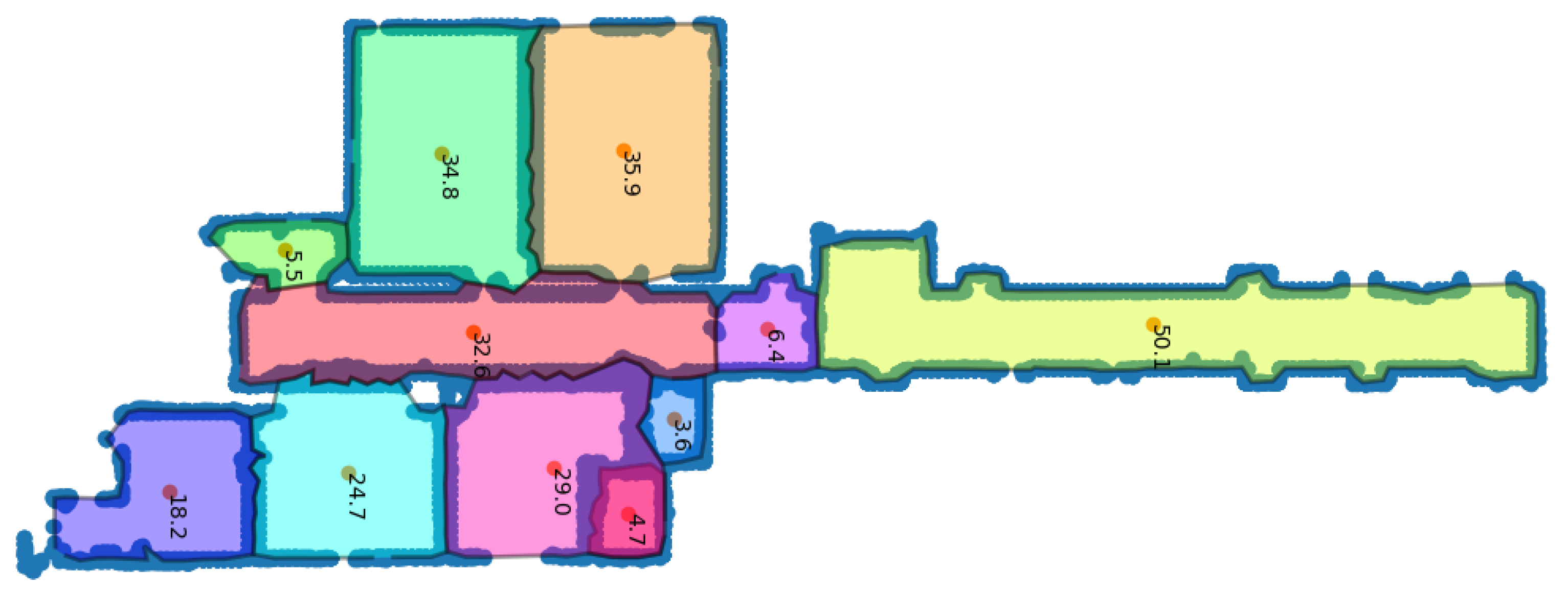
We provide further results here. In
Figure A1, the full reconstruction of the available apartments for all the rooms can be seen. The first one is the Redwood and the second the Freiburg apartment. Note that for the second one, we removed the reflection points to keep the dimension small.
Figure A1.
Full apartment with features. Reflections were not included to keep image size small.
Figure A1.
Full apartment with features. Reflections were not included to keep image size small.
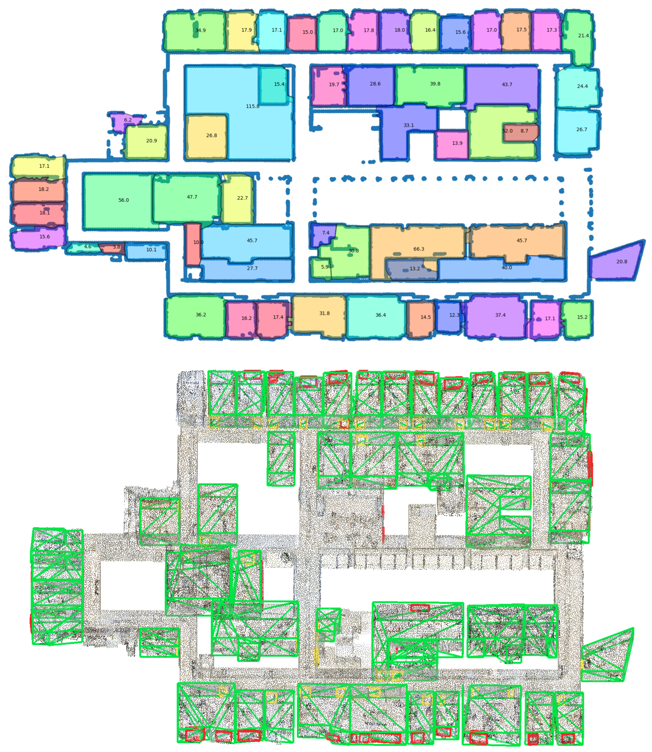
The detected rooms for the entirety of Area 5 from the S3DIS dataset are shown in
Figure A2. The top image shows the points detected as a wall and the contours describing the candidate rooms with the area in square meters. The lower image shows the reconstructed rooms with the additional doors (yellow) and windows (red).
Figure A2.
Full S3DIS Area 5.
Figure A2.
Full S3DIS Area 5.
References
- Chen, X.; Ma, H.; Wan, J.; Li, B.; Xia, T. Multi-View 3D Object Detection Network for Autonomous Driving. arXiv 2016, arXiv:1611.07759. [Google Scholar]
- Liang, M.; Yang, B.; Wang, S.; Urtasun, R. Deep Continuous Fusion for Multi-Sensor 3D Object Detection. arXiv 2020, arXiv:2012.10992. [Google Scholar]
- Cordts, M.; Omran, M.; Ramos, S.; Rehfeld, T.; Enzweiler, M.; Benenson, R.; Franke, U.; Roth, S.; Schiele, B. The Cityscapes Dataset for Semantic Urban Scene Understanding. arXiv 2016, arXiv:1604.01685v2. [Google Scholar]
- Merkle, D.; Frey, C.; Reiterer, A. Fusion of ground penetrating radar and laser scanning for infrastructure mapping. J. Appl. Geod. 2021, 15, 31–45. [Google Scholar] [CrossRef]
- Reiterer, A.; Wäschle, K.; Störk, D.; Leydecker, A.; Gitzen, N. Fully Automated Segmentation of 2D and 3D Mobile Mapping Data for Reliable Modeling of Surface Structures Using Deep Learning. Remote Sens. 2020, 12, 2530. [Google Scholar] [CrossRef]
- Merkle, D.; Schmitt, A.; Reiterer, A. Concept of an autonomous mobile robotic system for bridge inspection. In Proceedings of the SPIE Remote Sensing 2020, Edinburgh, UK, 21–24 September 2020. [Google Scholar] [CrossRef]
- von Olshausen, P.; Roetner, M.; Koch, C.; Reiterer, A. Multimodal measurement system for road analysis and surveying of road surroundings. In Proceedings of the Automated Visual Inspection and Machine Vision IV; Beyerer, J., Heizmann, M., Eds.; International Society for Optics and Photonics, SPIE: Bellingham, WA, USA, 2021; Volume 11787, pp. 72–78. [Google Scholar]
- Çiçek, Ö.; Abdulkadir, A.; Lienkamp, S.S.; Brox, T.; Ronneberger, O. 3D U-Net: Learning Dense Volumetric Segmentation from Sparse Annotation. arXiv 2016, arXiv:1606.06650. [Google Scholar]
- Bosché, F.; Ahmed, M.; Turkan, Y.; Haas, C.T.; Haas, R. The value of integrating Scan-to-BIM and Scan-vs-BIM techniques for construction monitoring using laser scanning and BIM: The case of cylindrical MEP components. Autom. Constr. 2015, 49, 201–213. [Google Scholar] [CrossRef]
- Turner, E.L.; Zakhor, A. Floor plan generation and room labeling of indoor environments from laser range data. In Proceedings of the 2014 International Conference on Computer Graphics Theory and Applications (GRAPP), Lisbon, Portugal, 5–8 January 2014; pp. 1–12. [Google Scholar]
- Mura, C.; Mattausch, O.; Jaspe Villanueva, A.; Gobbetti, E.; Pajarola, R. Automatic room detection and reconstruction in cluttered indoor environments with complex room layouts. Comput. Graph. 2014, 44, 20–32. [Google Scholar] [CrossRef]
- Ochmann, S.; Vock, R.; Wessel, R.; Klein, R. Automatic reconstruction of parametric building models from indoor point clouds. Comput. Graph. 2016, 54, 94–103. [Google Scholar] [CrossRef]
- Croce, V.; Caroti, G.; De Luca, L.; Jacquot, K.; Piemonte, A.; Véron, P. From the Semantic Point Cloud to Heritage-Building Information Modeling: A Semiautomatic Approach Exploiting Machine Learning. Remote Sens. 2021, 13, 461. [Google Scholar] [CrossRef]
- Uuganbayar Gankhuyag, J.H.H. Automatic BIM Indoor Modelling from Unstructured Point Clouds Using a Convolutional Neural Network. Intell. Autom. Soft Comput. 2021, 28, 133–152. [Google Scholar] [CrossRef]
- Tang, S.; Li, X.; Zheng, X.; Wu, B.; Wang, W.; Zhang, Y. BIM generation from 3D point clouds by combining 3D deep learning and improved morphological approach. Autom. Constr. 2022, 141, 104422. [Google Scholar] [CrossRef]
- Ahmed, S.; Liwicki, M.; Weber, M.; Dengel, A. Automatic Room Detection and Room Labeling from Architectural Floor Plans. In Proceedings of the 2012 10th IAPR International Workshop on Document Analysis Systems, Gold Coast, QLD, Australia, 27–29 March 2012; pp. 339–343. [Google Scholar] [CrossRef]
- Li, M.; Wonka, P.; Nan, L. Manhattan-World Urban Reconstruction from Point Clouds. In Proceedings of the Computer Vision–ECCV 2016, Amsterdam, The Netherlands, 11–14 October 2016; Leibe, B., Matas, J., Sebe, N., Welling, M., Eds.; Springer International Publishing: Cham, Switzerland, 2016; pp. 54–69. [Google Scholar]
- Coughlan, J.M.; Yuille, A.L. The Manhattan World Assumption: Regularities in Scene Statistics which Enable Bayesian Inference. In Proceedings of the NIPS, Denver, CO, USA, 27 November–2 December 2000; pp. 809–815. [Google Scholar]
- Nan, L.; Wonka, P. PolyFit: Polygonal Surface Reconstruction from Point Clouds. In Proceedings of the 2017 IEEE International Conference on Computer Vision (ICCV), Venice, Italy, 22–29 October 2017; pp. 2372–2380. [Google Scholar] [CrossRef]
- Guo, Y.; Wang, H.; Hu, Q.; Liu, H.; Liu, L.; Bennamoun, M. Deep Learning for 3D Point Clouds: A Survey. arXiv 2019, arXiv:1912.12033. [Google Scholar] [CrossRef]
- Hu, Q.; Yang, B.; Xie, L.; Rosa, S.; Guo, Y.; Wang, Z.; Trigoni, N.; Markham, A. RandLA-Net: Efficient Semantic Segmentation of Large-Scale Point Clouds. arXiv 2020, arXiv:1911.11236. [Google Scholar]
- Zhao, H.; Jiang, L.; Jia, J.; Torr, P.H.; Koltun, V. Point transformer. In Proceedings of the IEEE/CVF International Conference on Computer Vision, Virtual, 11–17 October 2021; pp. 16259–16268. [Google Scholar]
- Çiçek, Ö.; Abdulkadir, A.; Lienkamp, S.; Brox, T.; Ronneberger, O. 3D U-Net: Learning Dense Volumetric Segmentation from Sparse Annotation. In Proceedings of the Medical Image Computing and Computer-Assisted Intervention (MICCAI), Athens, Greece, 17–21 October 2016; Springer: Berlin/Heidelberg, Germany, 2016; Volume 9901, pp. 424–432. [Google Scholar]
- Weinmann, M.; Jutzi, B.; Mallet, C. Feature relevance assessment for the semantic interpretation of 3D point cloud data. In Proceedings of the ISPRS Workshop Laser Scanning 2013, ISPRS Annals of the Photogrammetry, Remote Sensing and Spatial Information Sciences, Antalya, Turkey, 11–13 November 2013; Volume II-5/W2, pp. 313–318. [Google Scholar] [CrossRef]
- Hackel, T.; Wegner, J.; Schindler, K. Contour Detection in Unstructured 3D Point Clouds. In Proceedings of the 2016 IEEE Conference on Computer Vision and Pattern Recognition (CVPR), Las Vegas, NV, USA, 27–30 June 2016; pp. 1610–1618. [Google Scholar] [CrossRef]
- Dijkstra, E. A Note on Two Problems in Connexion with Graphs. Numer. Math. 1959, 1, 269–271. [Google Scholar] [CrossRef]
- Goldman, R.N. IV.1—Area of planar polygons and volume of polyhedra. In Graphics Gems II; Arvo, J., Ed.; Morgan Kaufmann: San Diego, CA, USA, 1991; pp. 170–171. [Google Scholar] [CrossRef]
- Schnabel, R.; Wahl, R.; Klein, R. Efficient RANSAC for Point-Cloud Shape Detection. Comput. Graph. Forum 2007, 26, 214–226. [Google Scholar] [CrossRef]
- Ester, M.; Kriegel, H.P.; Sander, J.; Xu, X. Density-Based Clustering in Spatial Databases: The Algorithm GDBSCAN and Its Applications. In Proceedings of the 2nd International Conference on Knowledge Discovery and Data Mining, Portland, OR, USA, 2–4 August 1996. [Google Scholar]
- Hotelling, H. Analysis of a complex of statistical variables into principal components. J. Educ. Psychol. 1933, 24, 498–520. [Google Scholar] [CrossRef]
- Armeni, I.; Sener, O.; Zamir, A.R.; Jiang, H.; Brilakis, I.; Fischer, M.; Savarese, S. 3D Semantic Parsing of Large-Scale Indoor Spaces. In Proceedings of the IEEE International Conference on Computer Vision and Pattern Recognition, Las Vegas, NV, USA, 27–30 June 2016. [Google Scholar]
- Park, J.; Zhou, Q.Y.; Koltun, V. Colored Point Cloud Registration Revisited. In Proceedings of the ICCV, Venice, Italy, 22–29 October 2017. [Google Scholar]
- NavVis. NavVis VLX Point Cloud Data. Available online: https://www.navvis.com/resources/specifications/navvis-vlx-point-cloud-office (accessed on 16 November 2022).
- Khoshelham, K.; Díaz Vilariño, L.; Peter, M.; Kang, Z.; Acharya, D. The isprs benchmark on indoor modelling. Int. Arch. Photogramm. Remote Sens. Spat. Inf. Sci. 2017, XLII-2/W7, 367–372. [Google Scholar] [CrossRef]
- Zhou, Q.Y.; Park, J.; Koltun, V. Open3D: A Modern Library for 3D Data Processing. arXiv 2018, arXiv:1801.09847. [Google Scholar]
- Pedregosa, F.; Varoquaux, G.; Gramfort, A.; Michel, V.; Thirion, B.; Grisel, O.; Blondel, M.; Prettenhofer, P.; Weiss, R.; Dubourg, V.; et al. Scikit-learn: Machine Learning in Python. J. Mach. Learn. Res. 2011, 12, 2825–2830. [Google Scholar]
Figure 1.
Visualization of point clouds captured by different sensors. (a) Leica Geosystems RTC360, (b) Leica Geosystems BLK2GO, (c) Apple iPad Pro, and (d) Matterport Pro2.
Figure 1.
Visualization of point clouds captured by different sensors. (a) Leica Geosystems RTC360, (b) Leica Geosystems BLK2GO, (c) Apple iPad Pro, and (d) Matterport Pro2.
Figure 2.
Stages showing the feature enriched downsampling strategy. (a) Original points , (b) voxeled points, (c) calculated covariance, and (d) resulting point cloud .
Figure 2.
Stages showing the feature enriched downsampling strategy. (a) Original points , (b) voxeled points, (c) calculated covariance, and (d) resulting point cloud .
Figure 3.
Stages showing the different parts of room fitting algorithm. The top row shows the projection into 2D while the row below shows the step reprojected into 3D. The prediction and remaining points belonging to walls are shown in (a). In (b), the detected lines (2D) and the resulting faces (3D) are shown. The bounded line segments and faces are visualized in (c). The closed line segments and final faces can be seen in (d).
Figure 4.
Visualization of different calculated features. The color is scaled from blue, green, and yellow to red for the feature value of range
. The ceiling, as well as one wall, is removed for easier visualization. The names are described in
Table 1.
Figure 4.
Visualization of different calculated features. The color is scaled from blue, green, and yellow to red for the feature value of range
. The ceiling, as well as one wall, is removed for easier visualization. The names are described in
Table 1.
Figure 5.
Different stages for extracting possible room candidates. The Redwood, the S3DIS, the RTC360, the BLK2Go, and the VLX data are displayed in order from top to bottom. The prediction of all points can be seen in (a). The ceiling has been removed for easier visualization. In (b), the created graph and the corresponding edges are shown. All vertices larger than some threshold are removed creating multiple subgraphs in (c). Better connections are searched for and a new graph is constructed (d). Cycles are searched for in the resulting graph and path patches are used to define the room contours (e).
Figure 6.
Different stages for whole pipeline. The Redwood, the S3DIS, the RTC360, the BLK2Go, and the VLX data are displayed in order from top to bottom. The prediction of the defined base elements is shown in (a). In (b), all points are assigned to RoIs by the described graph search. The RoIs fitted by polygons are visualized in (c). The fitted polygons and the raw points are shown in (d).
Figure 7.
Distance between points belonging to classes used for the polygon extraction and the final extracted room polygons. The number of points is normalized with respect to the number of points in each dataset.
Figure 7.
Distance between points belonging to classes used for the polygon extraction and the final extracted room polygons. The number of points is normalized with respect to the number of points in each dataset.
Figure 8.
Quantitative comparison between the automatically generated (green) and the manual, human-reconstructed geometry (red). The points predicted by the NN as a wall are displayed in blue. (a) Easy room, (b) small room with fine details, and (c) large floor with corners.
Figure 8.
Quantitative comparison between the automatically generated (green) and the manual, human-reconstructed geometry (red). The points predicted by the NN as a wall are displayed in blue. (a) Easy room, (b) small room with fine details, and (c) large floor with corners.
Figure 9.
Different sensor inputs and the corresponding reconstructed room with additional features. Each row shows a point cloud from a different sensor. Starting with the Redwood, the S3DIS, the RTC360, and, finally, the VLX data. The first column (a) shows the colorized point cloud for easier visualization. The second column (b) is the final digital model, which was created by our proposed method. In the last column (c), we have superimposed the regenerated model and the original point cloud.
Table 1.
Geometrical features calculated by the eigenvalues of the covariance matrix.
Table 1.
Geometrical features calculated by the eigenvalues of the covariance matrix.
| Planarity | | |
| Linearity | | |
| Sphericity | | |
| Surface variation | | |
| Sum of eigenvalues | | |
| Omnivariance | | |
| Eigentropy | | |
| Anisotropy | | |
Table 2.
Runtime in ms using Open3D voxel downsampling, and our approach to downsample and include the feature calculation and the Nearest Neighbor calculation using Open3D and Scikit-Learn. For downsampling, we chose a voxel size of m. All experiments were conducted using S3DIS Area 5 data, which contains 68 point clouds with a total amount of 78,719,063 points. Note that the calculation for the covariance matrix and the eigenvalues are not included within the kNN time but in our approach.
| | Open3D | Ours | Open3D kNN | Scikit-Learn kNN |
|---|
| min | 7.57 | 18.62 | 116.67 | 704.27 |
| avrg | 50.1 | 159.35 | 928.12 | 5197.86 |
| max | 218.7 | 694.4 | 4866.96 | 22,565.6 |
Table 3.
Semantic segmentation results for different architectures. The first part shows the results using color information and the second part shows the results using the proposed geometrical features. The first section for the given input names the IoU on S3DIS evaluated on Area 5. The second section indicates the results of our internally generated data using an RTC360 scanner.
| Input | Method | Clutter | Ceiling | Floor | Wall | Door | Window | Door Leaf | mIoU |
|---|
| RGB | PointTransformer | 0.8 | 0.9 | 0.98 | 0.74 | 0.49 | 0.47 | 0.57 | 0.71 |
| | RandLA-Net | 0.84 | 0.93 | 0.98 | 0.81 | 0.34 | 0.48 | 0.08 | 0.65 |
| | 3DConv | 0.63 | 0.84 | 0.86 | 0.62 | 0.36 | 0.21 | 0.2 | 0.53 |
| RGB | PointTransformer | 0.4 | 0.55 | 0.83 | 0.67 | 0.19 | 0.02 | 0.13 | 0.4 |
| | RandLA-Net | 0.39 | 0.64 | 0.95 | 0.76 | 0.12 | 0.01 | 0.0 | 0.41 |
| | 3DConv | 0.6 | 0.82 | 0.82 | 0.73 | 0.12 | 0.03 | 0.05 | 0.45 |
| Geo | PointTransformer | 0.82 | 0.92 | 0.98 | 0.77 | 0.54 | 0.48 | 0.67 | 0.74 |
| | RandLA-Net | 0.85 | 0.93 | 0.98 | 0.78 | 0.45 | 0.34 | 0.66 | 0.71 |
| | 3DConv | 0.63 | 0.86 | 0.86 | 0.64 | 0.33 | 0.29 | 0.37 | 0.57 |
| Geo | PointTransformer | 0.42 | 0.53 | 0.73 | 0.73 | 0.2 | 0.02 | 0.05 | 0.39 |
| | RandLA-Net | 0.48 | 0.66 | 0.95 | 0.63 | 0.14 | 0.02 | 0.1 | 0.43 |
| | 3DConv | 0.59 | 0.81 | 0.87 | 0.77 | 0.17 | 0.04 | 0.11 | 0.48 |
Table 4.
The number of detected regions of interest compared to the real number of existing rooms.
Table 4.
The number of detected regions of interest compared to the real number of existing rooms.
| | Redwood | S3DIS | RTC | BLK2Go | vlx |
|---|
| Rooms | 3 | 12 | 16 | 6 | 6 |
| Detected | 3 | 14 | 21 | 6 | 7 |
| After post-processing | 3 | 12 | 19 | 6 | 6 |
| Disclaimer/Publisher’s Note: The statements, opinions and data contained in all publications are solely those of the individual author(s) and contributor(s) and not of MDPI and/or the editor(s). MDPI and/or the editor(s) disclaim responsibility for any injury to people or property resulting from any ideas, methods, instructions or products referred to in the content. |
© 2023 by the authors. Licensee MDPI, Basel, Switzerland. This article is an open access article distributed under the terms and conditions of the Creative Commons Attribution (CC BY) license (https://creativecommons.org/licenses/by/4.0/).


